Accessing databases using dbplyr
library(tidyverse)
set.seed(1234)

theme_set(theme_minimal())
So far we’ve only worked with data stored locally in-memory as data frames. However there are also situations where you want to work with data stored in an external database. Databases are generally stored remotely on-disk, as opposed to in memory. If your data is already stored in a database, or if you have too much data to fit it all into memory simultaneously, you need a way to access it. Fortunately for you, dplyr offers support for on-disk databases through dbplyr.
SQL
Structured Query Language (SQL) is a means of communicating with a relational database management system. There are different types of SQL databases which offer varying functionality:
Databases can also be stored across many platforms. Some types of databases (such as SQLite) can be stored as a single file and loaded in-memory like a data frame. However for large or extremely complex databases, a local computer is insufficient. Instead, one uses a distributed computing platform to store their database in the cloud. Examples include the UChicago Research Computing Center (RCC), Amazon Web Services, and Google Cloud Platform. Note that hosting platforms not typically free (though you can request an account with RCC as a student).
Getting started with SQLite
First you need to install dbplyr:
install.packages("dbplyr")Depending on the type of database, you also need to install the appropriate database interface (DBI) package. The DBI package provides the necessary interface between the database and dplyr. Five commonly used backends are:
RMySQLconnects to MySQL and MariaDBRPostgreSQLconnects to Postgres and Redshift.RSQLiteembeds a SQLite database.odbcconnects to many commercial databases via the open database connectivity protocol.bigrqueryconnects to Google’s BigQuery.
Connecting to the database
Let’s create a local SQLite database using the flights data.
library(dplyr)
my_db <- DBI::dbConnect(RSQLite::SQLite(), path = ":memory:")
The first argument to DBI::dbConnect() is the database backend. SQLite only requires one other argument: the path to the database. Here, we use :memory: to create a temporary in-memory database.
To add data to the database, use copy_to(). Let’s stock the database with nycflights13::flights:
library(nycflights13)
copy_to(my_db,
        flights,
        temporary = FALSE,
        indexes = list(
          c("year", "month", "day"),
          "carrier",
          "tailnum"
        )
)
Now that we copied the data, we can use tbl() to reference a specific table inside the database:
flights_db <- tbl(my_db, "flights")
flights_db
## # Source: table<flights> [?? x 19]
## # Database: sqlite 3.19.3 []
## year month day dep_time sched_dep_time dep_delay arr_time
## <int> <int> <int> <int> <int> <dbl> <int>
## 1 2013 1 1 517 515 2 830
## 2 2013 1 1 533 529 4 850
## 3 2013 1 1 542 540 2 923
## 4 2013 1 1 544 545 -1 1004
## 5 2013 1 1 554 600 -6 812
## 6 2013 1 1 554 558 -4 740
## 7 2013 1 1 555 600 -5 913
## 8 2013 1 1 557 600 -3 709
## 9 2013 1 1 557 600 -3 838
## 10 2013 1 1 558 600 -2 753
## # ... with more rows, and 12 more variables: sched_arr_time <int>,
## # arr_delay <dbl>, carrier <chr>, flight <int>, tailnum <chr>,
## # origin <chr>, dest <chr>, air_time <dbl>, distance <dbl>, hour <dbl>,
## # minute <dbl>, time_hour <dbl>Basic verbs
select(flights_db, year:day, dep_delay, arr_delay)## # Source: lazy query [?? x 5]
## # Database: sqlite 3.19.3 []
## year month day dep_delay arr_delay
## <int> <int> <int> <dbl> <dbl>
## 1 2013 1 1 2 11
## 2 2013 1 1 4 20
## 3 2013 1 1 2 33
## 4 2013 1 1 -1 -18
## 5 2013 1 1 -6 -25
## 6 2013 1 1 -4 12
## 7 2013 1 1 -5 19
## 8 2013 1 1 -3 -14
## 9 2013 1 1 -3 -8
## 10 2013 1 1 -2 8
## # ... with more rowsfilter(flights_db, dep_delay > 240)## # Source: lazy query [?? x 19]
## # Database: sqlite 3.19.3 []
## year month day dep_time sched_dep_time dep_delay arr_time
## <int> <int> <int> <int> <int> <dbl> <int>
## 1 2013 1 1 848 1835 853 1001
## 2 2013 1 1 1815 1325 290 2120
## 3 2013 1 1 1842 1422 260 1958
## 4 2013 1 1 2115 1700 255 2330
## 5 2013 1 1 2205 1720 285 46
## 6 2013 1 1 2343 1724 379 314
## 7 2013 1 2 1332 904 268 1616
## 8 2013 1 2 1412 838 334 1710
## 9 2013 1 2 1607 1030 337 2003
## 10 2013 1 2 2131 1512 379 2340
## # ... with more rows, and 12 more variables: sched_arr_time <int>,
## # arr_delay <dbl>, carrier <chr>, flight <int>, tailnum <chr>,
## # origin <chr>, dest <chr>, air_time <dbl>, distance <dbl>, hour <dbl>,
## # minute <dbl>, time_hour <dbl>arrange(flights_db, year, month, day)## # Source: table<flights> [?? x 19]
## # Database: sqlite 3.19.3 []
## # Ordered by: year, month, day
## year month day dep_time sched_dep_time dep_delay arr_time
## <int> <int> <int> <int> <int> <dbl> <int>
## 1 2013 1 1 517 515 2 830
## 2 2013 1 1 533 529 4 850
## 3 2013 1 1 542 540 2 923
## 4 2013 1 1 544 545 -1 1004
## 5 2013 1 1 554 600 -6 812
## 6 2013 1 1 554 558 -4 740
## 7 2013 1 1 555 600 -5 913
## 8 2013 1 1 557 600 -3 709
## 9 2013 1 1 557 600 -3 838
## 10 2013 1 1 558 600 -2 753
## # ... with more rows, and 12 more variables: sched_arr_time <int>,
## # arr_delay <dbl>, carrier <chr>, flight <int>, tailnum <chr>,
## # origin <chr>, dest <chr>, air_time <dbl>, distance <dbl>, hour <dbl>,
## # minute <dbl>, time_hour <dbl>mutate(flights_db, speed = air_time / distance)## # Source: lazy query [?? x 20]
## # Database: sqlite 3.19.3 []
## year month day dep_time sched_dep_time dep_delay arr_time
## <int> <int> <int> <int> <int> <dbl> <int>
## 1 2013 1 1 517 515 2 830
## 2 2013 1 1 533 529 4 850
## 3 2013 1 1 542 540 2 923
## 4 2013 1 1 544 545 -1 1004
## 5 2013 1 1 554 600 -6 812
## 6 2013 1 1 554 558 -4 740
## 7 2013 1 1 555 600 -5 913
## 8 2013 1 1 557 600 -3 709
## 9 2013 1 1 557 600 -3 838
## 10 2013 1 1 558 600 -2 753
## # ... with more rows, and 13 more variables: sched_arr_time <int>,
## # arr_delay <dbl>, carrier <chr>, flight <int>, tailnum <chr>,
## # origin <chr>, dest <chr>, air_time <dbl>, distance <dbl>, hour <dbl>,
## # minute <dbl>, time_hour <dbl>, speed <dbl>summarise(flights_db, delay = mean(dep_time))## # Source: lazy query [?? x 1]
## # Database: sqlite 3.19.3 []
## delay
## <dbl>
## 1 1349.11The commands are generally the same as you would use in dplyr. The only difference is that dplyr converts your R commands into SQL syntax:
select(flights_db, year:day, dep_delay, arr_delay) %>%
  show_query()
## <SQL>
## SELECT `year` AS `year`, `month` AS `month`, `day` AS `day`, `dep_delay` AS `dep_delay`, `arr_delay` AS `arr_delay`
## FROM `flights`dbplyr is also lazy:
- It never pulls data into R unless you explicitly ask for it
- It delays doing any work until the last possible moment: it collects together everything you want to do and then sends it to the database in one step.
c1 <- filter(flights_db, year == 2013, month == 1, day == 1)
c2 <- select(c1, year, month, day, carrier, dep_delay, air_time, distance)
c3 <- mutate(c2, speed = distance / air_time * 60)
c4 <- arrange(c3, year, month, day, carrier)
Nothing has actually gone to the database yet.
c4## # Source: lazy query [?? x 8]
## # Database: sqlite 3.19.3 []
## # Ordered by: year, month, day, carrier
## year month day carrier dep_delay air_time distance speed
## <int> <int> <int> <chr> <dbl> <dbl> <dbl> <dbl>
## 1 2013 1 1 9E 0 189 1029 326.6667
## 2 2013 1 1 9E -9 57 228 240.0000
## 3 2013 1 1 9E -3 68 301 265.5882
## 4 2013 1 1 9E -6 57 209 220.0000
## 5 2013 1 1 9E -8 66 264 240.0000
## 6 2013 1 1 9E 0 40 184 276.0000
## 7 2013 1 1 9E 6 146 740 304.1096
## 8 2013 1 1 9E 0 139 665 287.0504
## 9 2013 1 1 9E -8 150 765 306.0000
## 10 2013 1 1 9E -6 41 187 273.6585
## # ... with more rowsNow we finally communicate with the database, but only retrieved the first 10 rows (notice the ?? in query [?? x 8]). This is a built-in feature to avoid downloading an extremely large data frame our machine cannot handle. To obtain the full results, use collect():
collect(c4)## # A tibble: 842 x 8
## year month day carrier dep_delay air_time distance speed
## <int> <int> <int> <chr> <dbl> <dbl> <dbl> <dbl>
## 1 2013 1 1 9E 0 189 1029 326.6667
## 2 2013 1 1 9E -9 57 228 240.0000
## 3 2013 1 1 9E -3 68 301 265.5882
## 4 2013 1 1 9E -6 57 209 220.0000
## 5 2013 1 1 9E -8 66 264 240.0000
## 6 2013 1 1 9E 0 40 184 276.0000
## 7 2013 1 1 9E 6 146 740 304.1096
## 8 2013 1 1 9E 0 139 665 287.0504
## 9 2013 1 1 9E -8 150 765 306.0000
## 10 2013 1 1 9E -6 41 187 273.6585
## # ... with 832 more rowsGoogle Bigquery
Google Bigquery is a distributed cloud platform for data warehousing and analytics. It can scan terabytes of data in seconds and petabytes in minutes. It has flexible pricing that scales depending on your demand on their resources, and could cost as little as pennies, though depending on your computation may cost more.
Interacting with Google Bigquery via dplyr
Google Bigquery hosts several public (and free) datasets. One is the NYC Taxi and Limousine Trips dataset, which contains trip records from all trips completed in yellow and green taxis in NYC from 2009 to 2015. Records include fields capturing pick-up and drop-off dates/times, pick-up and drop-off locations, trip distances, itemized fares, rate types, payment types, and driver-reported passenger counts. The dataset itself is hundreds of gigabytes and could never be loaded on a desktop machine. But fortunately we can harness the power of the cloud.
To connect to the database, we use the bigrquery library and bigrquery::bigquery():
library(bigrquery)

taxi <- DBI::dbConnect(bigrquery::bigquery(),
                       project = "nyc-tlc",
                       dataset = "yellow",
                       billing = getOption("bigquery_id"))
taxi
## <BigQueryConnection>
## Dataset: nyc-tlc:yellowproject- the project that is hosting the datadataset- the specific database to be accessedbilling- your unique id to access the data (and be charged if you run too many queries or use to much computing power). You need to create an account in order to use BigQuery, even if you want to access the free datasets. I stored mine in.Rprofileusingoptions().1
First lets determine in 2014, how many trips per taken each month in yellow cabs? The SQL syntax is:
SELECT
  LEFT(STRING(pickup_datetime), 7) month,
  COUNT(*) trips
FROM
  [nyc-tlc:yellow.trips]
WHERE
  YEAR(pickup_datetime) = 2014
GROUP BY
  1
ORDER BY
  1
In dbplyr, we use:
system.time({
  trips_by_month <- taxi %>%
    tbl("trips") %>%
    filter(year(pickup_datetime) == 2014) %>%
    mutate(month = month(pickup_datetime)) %>%
    count(month) %>%
    arrange(month) %>%
    collect()
})
## user system elapsed
## 0.270 0.013 3.657trips_by_month## # A tibble: 12 x 2
## month n
## <int> <int>
## 1 1 13782492
## 2 2 13063791
## 3 3 15428127
## 4 4 14618759
## 5 5 14774041
## 6 6 13813029
## 7 7 13106365
## 8 8 12688877
## 9 9 13374016
## 10 10 14232487
## 11 11 13218216
## 12 12 13014161What about the average speed per hour of day in yellow cabs?
system.time({
  speed_per_hour <- taxi %>%
    tbl("trips") %>%
    mutate(hour = hour(pickup_datetime),
           trip_duration = (dropoff_datetime - pickup_datetime) /
             3600000000) %>%
    mutate(speed = trip_distance / trip_duration) %>%
    filter(fare_amount / trip_distance >= 2,
           fare_amount / trip_distance <= 10) %>%
    group_by(hour) %>%
    summarize(speed = mean(speed)) %>%
    arrange(hour) %>%
    collect()
})
## user system elapsed
## 0.359 0.015 1.402ggplot(speed_per_hour, aes(hour, speed)) +
geom_line() +
labs(title = "Average Speed of NYC Yellow Taxis",
x = "Hour of day",
y = "Average speed, in MPH")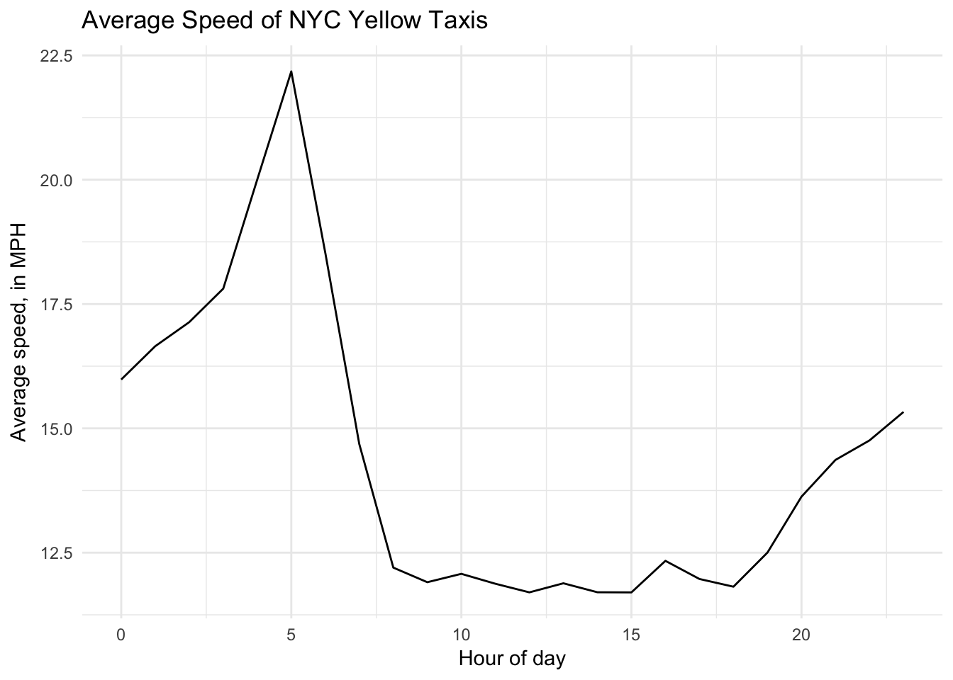
Finally, what is the average speed by day of the week?
system.time({
  speed_per_day <- taxi %>%
    tbl("trips") %>%
    mutate(hour = hour(pickup_datetime),
           day = dayofweek(pickup_datetime),
           trip_duration = (dropoff_datetime - pickup_datetime) /
             3600000000) %>%
    mutate(speed = trip_distance / trip_duration) %>%
    filter(fare_amount / trip_distance >= 2,
           fare_amount / trip_distance <= 10,
           hour >= 8,
           hour <= 18) %>%
    group_by(day) %>%
    summarize(speed = mean(speed)) %>%
    arrange(day) %>%
    collect()
})
## user system elapsed
## 0.384 0.015 1.098speed_per_day## # A tibble: 7 x 2
## day speed
## <int> <dbl>
## 1 1 14.29703
## 2 2 12.21557
## 3 3 11.11933
## 4 4 10.93281
## 5 5 10.97011
## 6 6 11.24917
## 7 7 13.09473Acknowledgments
Session Info
devtools::session_info()## setting value
## version R version 3.4.3 (2017-11-30)
## system x86_64, darwin15.6.0
## ui X11
## language (EN)
## collate en_US.UTF-8
## tz America/Chicago
## date 2018-04-24
##
## package * version date source
## assertthat 0.2.0 2017-04-11 CRAN (R 3.4.0)
## backports 1.1.2 2017-12-13 CRAN (R 3.4.3)
## base * 3.4.3 2017-12-07 local
## bindr 0.1.1 2018-03-13 CRAN (R 3.4.3)
## bindrcpp 0.2.2.9000 2018-04-08 Github (krlmlr/bindrcpp@bd5ae73)
## bit 1.1-12 2014-04-09 CRAN (R 3.4.0)
## bit64 0.9-7 2017-05-08 CRAN (R 3.4.0)
## blob 1.1.1 2018-03-25 CRAN (R 3.4.4)
## broom 0.4.4 2018-03-29 CRAN (R 3.4.3)
## cellranger 1.1.0 2016-07-27 CRAN (R 3.4.0)
## cli 1.0.0 2017-11-05 CRAN (R 3.4.2)
## colorspace 1.3-2 2016-12-14 CRAN (R 3.4.0)
## compiler 3.4.3 2017-12-07 local
## crayon 1.3.4 2017-10-03 Github (gaborcsardi/crayon@b5221ab)
## datasets * 3.4.3 2017-12-07 local
## DBI 0.8 2018-03-02 CRAN (R 3.4.3)
## devtools 1.13.5 2018-02-18 CRAN (R 3.4.3)
## digest 0.6.15 2018-01-28 CRAN (R 3.4.3)
## dplyr * 0.7.4.9003 2018-04-08 Github (tidyverse/dplyr@b7aaa95)
## evaluate 0.10.1 2017-06-24 CRAN (R 3.4.1)
## forcats * 0.3.0 2018-02-19 CRAN (R 3.4.3)
## foreign 0.8-69 2017-06-22 CRAN (R 3.4.3)
## ggplot2 * 2.2.1.9000 2018-04-24 Github (tidyverse/ggplot2@3c9c504)
## glue 1.2.0 2017-10-29 CRAN (R 3.4.2)
## graphics * 3.4.3 2017-12-07 local
## grDevices * 3.4.3 2017-12-07 local
## grid 3.4.3 2017-12-07 local
## gtable 0.2.0 2016-02-26 CRAN (R 3.4.0)
## haven 1.1.1 2018-01-18 CRAN (R 3.4.3)
## hms 0.4.2 2018-03-10 CRAN (R 3.4.3)
## htmltools 0.3.6 2017-04-28 CRAN (R 3.4.0)
## httr 1.3.1 2017-08-20 CRAN (R 3.4.1)
## jsonlite 1.5 2017-06-01 CRAN (R 3.4.0)
## knitr 1.20 2018-02-20 CRAN (R 3.4.3)
## lattice 0.20-35 2017-03-25 CRAN (R 3.4.3)
## lazyeval 0.2.1 2017-10-29 CRAN (R 3.4.2)
## lubridate 1.7.4 2018-04-11 CRAN (R 3.4.3)
## magrittr 1.5 2014-11-22 CRAN (R 3.4.0)
## memoise 1.1.0 2017-04-21 CRAN (R 3.4.0)
## methods * 3.4.3 2017-12-07 local
## mnormt 1.5-5 2016-10-15 CRAN (R 3.4.0)
## modelr 0.1.1 2017-08-10 local
## munsell 0.4.3 2016-02-13 CRAN (R 3.4.0)
## nlme 3.1-137 2018-04-07 CRAN (R 3.4.4)
## parallel 3.4.3 2017-12-07 local
## pillar 1.2.1 2018-02-27 CRAN (R 3.4.3)
## pkgconfig 2.0.1 2017-03-21 CRAN (R 3.4.0)
## plyr 1.8.4 2016-06-08 CRAN (R 3.4.0)
## psych 1.8.3.3 2018-03-30 CRAN (R 3.4.4)
## purrr * 0.2.4 2017-10-18 CRAN (R 3.4.2)
## R6 2.2.2 2017-06-17 CRAN (R 3.4.0)
## Rcpp 0.12.16 2018-03-13 CRAN (R 3.4.4)
## readr * 1.1.1 2017-05-16 CRAN (R 3.4.0)
## readxl 1.0.0 2017-04-18 CRAN (R 3.4.0)
## reshape2 1.4.3 2017-12-11 CRAN (R 3.4.3)
## rlang 0.2.0.9001 2018-04-24 Github (r-lib/rlang@82b2727)
## rmarkdown 1.9 2018-03-01 CRAN (R 3.4.3)
## rprojroot 1.3-2 2018-01-03 CRAN (R 3.4.3)
## RSQLite 2.1.0 2018-03-29 CRAN (R 3.4.4)
## rstudioapi 0.7 2017-09-07 CRAN (R 3.4.1)
## rvest 0.3.2 2016-06-17 CRAN (R 3.4.0)
## scales 0.5.0.9000 2018-04-24 Github (hadley/scales@d767915)
## stats * 3.4.3 2017-12-07 local
## stringi 1.1.7 2018-03-12 CRAN (R 3.4.3)
## stringr * 1.3.0 2018-02-19 CRAN (R 3.4.3)
## tibble * 1.4.2 2018-01-22 CRAN (R 3.4.3)
## tidyr * 0.8.0 2018-01-29 CRAN (R 3.4.3)
## tidyselect 0.2.4 2018-02-26 CRAN (R 3.4.3)
## tidyverse * 1.2.1 2017-11-14 CRAN (R 3.4.2)
## tools 3.4.3 2017-12-07 local
## utils * 3.4.3 2017-12-07 local
## withr 2.1.2 2018-04-24 Github (jimhester/withr@79d7b0d)
## xml2 1.2.0 2018-01-24 CRAN (R 3.4.3)
## yaml 2.1.18 2018-03-08 CRAN (R 3.4.4)This may not make sense to you. You will learn more about storing credentials next week in our unit on accessing data from the web.↩
This work is licensed under the CC BY-NC 4.0 Creative Commons License.