dplyr::group_by()

gapminder %>%
  group_by(continent) %>%
  summarize(n = n())

## # A tibble: 5 x 2
##   continent     n
##      <fctr> <int>
## 1    Africa   624
## 2  Americas   300
## 3      Asia   396
## 4    Europe   360
## 5   Oceania    24

gapminder %>%
  group_by(continent) %>%
  summarize(avg_lifeExp = mean(lifeExp))

## # A tibble: 5 x 2
##   continent avg_lifeExp
##      <fctr>       <dbl>
## 1    Africa    48.86533
## 2  Americas    64.65874
## 3      Asia    60.06490
## 4    Europe    71.90369
## 5   Oceania    74.32621

for loops

countries <- unique(gapminder$country)
lifeExp_models <- vector("list", length(countries))
names(lifeExp_models) <- countries

for(i in seq_along(countries)){
  lifeExp_models[[i]] <- lm(lifeExp ~ year,
                            data = filter(gapminder,
                                          country == countries[[i]]))
}
head(lifeExp_models)

## $Afghanistan
## 
## Call:
## lm(formula = lifeExp ~ year, data = filter(gapminder, country == 
##     countries[[i]]))
## 
## Coefficients:
## (Intercept)         year  
##   -507.5343       0.2753  
## 
## 
## $Albania
## 
## Call:
## lm(formula = lifeExp ~ year, data = filter(gapminder, country == 
##     countries[[i]]))
## 
## Coefficients:
## (Intercept)         year  
##   -594.0725       0.3347  
## 
## 
## $Algeria
## 
## Call:
## lm(formula = lifeExp ~ year, data = filter(gapminder, country == 
##     countries[[i]]))
## 
## Coefficients:
## (Intercept)         year  
##  -1067.8590       0.5693  
## 
## 
## $Angola
## 
## Call:
## lm(formula = lifeExp ~ year, data = filter(gapminder, country == 
##     countries[[i]]))
## 
## Coefficients:
## (Intercept)         year  
##   -376.5048       0.2093  
## 
## 
## $Argentina
## 
## Call:
## lm(formula = lifeExp ~ year, data = filter(gapminder, country == 
##     countries[[i]]))
## 
## Coefficients:
## (Intercept)         year  
##   -389.6063       0.2317  
## 
## 
## $Australia
## 
## Call:
## lm(formula = lifeExp ~ year, data = filter(gapminder, country == 
##     countries[[i]]))
## 
## Coefficients:
## (Intercept)         year  
##   -376.1163       0.2277

nest() and map()

# function to estimate linear model for gapminder subsets
le_vs_yr <- function(df) {
  lm(lifeExp ~ year, data = df)
}

# split data into nests
(gap_nested <- gapminder %>% 
   group_by(continent, country) %>% 
   nest())

## # A tibble: 142 x 3
##    continent     country              data
##       <fctr>      <fctr>            <list>
##  1      Asia Afghanistan <tibble [12 x 4]>
##  2    Europe     Albania <tibble [12 x 4]>
##  3    Africa     Algeria <tibble [12 x 4]>
##  4    Africa      Angola <tibble [12 x 4]>
##  5  Americas   Argentina <tibble [12 x 4]>
##  6   Oceania   Australia <tibble [12 x 4]>
##  7    Europe     Austria <tibble [12 x 4]>
##  8      Asia     Bahrain <tibble [12 x 4]>
##  9      Asia  Bangladesh <tibble [12 x 4]>
## 10    Europe     Belgium <tibble [12 x 4]>
## # ... with 132 more rows

# apply a linear model to each nested data frame
(gap_nested <- gap_nested %>% 
   mutate(fit = map(data, le_vs_yr)))

## # A tibble: 142 x 4
##    continent     country              data      fit
##       <fctr>      <fctr>            <list>   <list>
##  1      Asia Afghanistan <tibble [12 x 4]> <S3: lm>
##  2    Europe     Albania <tibble [12 x 4]> <S3: lm>
##  3    Africa     Algeria <tibble [12 x 4]> <S3: lm>
##  4    Africa      Angola <tibble [12 x 4]> <S3: lm>
##  5  Americas   Argentina <tibble [12 x 4]> <S3: lm>
##  6   Oceania   Australia <tibble [12 x 4]> <S3: lm>
##  7    Europe     Austria <tibble [12 x 4]> <S3: lm>
##  8      Asia     Bahrain <tibble [12 x 4]> <S3: lm>
##  9      Asia  Bangladesh <tibble [12 x 4]> <S3: lm>
## 10    Europe     Belgium <tibble [12 x 4]> <S3: lm>
## # ... with 132 more rows

# combine the results back into a single data frame
library(broom)
(gap_nested <- gap_nested %>% 
  mutate(tidy = map(fit, tidy)))

## # A tibble: 142 x 5
##    continent     country              data      fit                 tidy
##       <fctr>      <fctr>            <list>   <list>               <list>
##  1      Asia Afghanistan <tibble [12 x 4]> <S3: lm> <data.frame [2 x 5]>
##  2    Europe     Albania <tibble [12 x 4]> <S3: lm> <data.frame [2 x 5]>
##  3    Africa     Algeria <tibble [12 x 4]> <S3: lm> <data.frame [2 x 5]>
##  4    Africa      Angola <tibble [12 x 4]> <S3: lm> <data.frame [2 x 5]>
##  5  Americas   Argentina <tibble [12 x 4]> <S3: lm> <data.frame [2 x 5]>
##  6   Oceania   Australia <tibble [12 x 4]> <S3: lm> <data.frame [2 x 5]>
##  7    Europe     Austria <tibble [12 x 4]> <S3: lm> <data.frame [2 x 5]>
##  8      Asia     Bahrain <tibble [12 x 4]> <S3: lm> <data.frame [2 x 5]>
##  9      Asia  Bangladesh <tibble [12 x 4]> <S3: lm> <data.frame [2 x 5]>
## 10    Europe     Belgium <tibble [12 x 4]> <S3: lm> <data.frame [2 x 5]>
## # ... with 132 more rows

(gap_coefs <- gap_nested %>% 
   select(continent, country, tidy) %>% 
   unnest(tidy))

## # A tibble: 284 x 7
##    continent     country        term      estimate    std.error  statistic
##       <fctr>      <fctr>       <chr>         <dbl>        <dbl>      <dbl>
##  1      Asia Afghanistan (Intercept)  -507.5342716 40.484161954 -12.536613
##  2      Asia Afghanistan        year     0.2753287  0.020450934  13.462890
##  3    Europe     Albania (Intercept)  -594.0725110 65.655359062  -9.048348
##  4    Europe     Albania        year     0.3346832  0.033166387  10.091036
##  5    Africa     Algeria (Intercept) -1067.8590396 43.802200843 -24.379118
##  6    Africa     Algeria        year     0.5692797  0.022127070  25.727749
##  7    Africa      Angola (Intercept)  -376.5047531 46.583370599  -8.082385
##  8    Africa      Angola        year     0.2093399  0.023532003   8.895964
##  9  Americas   Argentina (Intercept)  -389.6063445  9.677729641 -40.258031
## 10  Americas   Argentina        year     0.2317084  0.004888791  47.395847
## # ... with 274 more rows, and 1 more variables: p.value <dbl>

Why use parallel computing

• Parallel computing imitates real life - in the real world, people use their brains to think in parallel - we multitask all the time without even thinking about it. Institutions are structured to process information in parallel, rather than in serial.
• It can be more efficient - by throwing more resources at a problem you can shorten the time to completion.
• You can tackle larger problems - more resources enables you to scale up the amount of data you process and potentially solve a larger problem.
• Distributed resources are cheaper than upgrading your own equipment. Why spend thousands of dollars beefing up your own laptop when you can instead rent computing resources from Google or Amazon for mere pennies?

Why not to use parallel computing

• Limits to efficiency gains - Amdahl’s law defines theoretical limits to how much you can speed up computations via parallel computing. Because of this, you achieve diminishing returns over time.

  

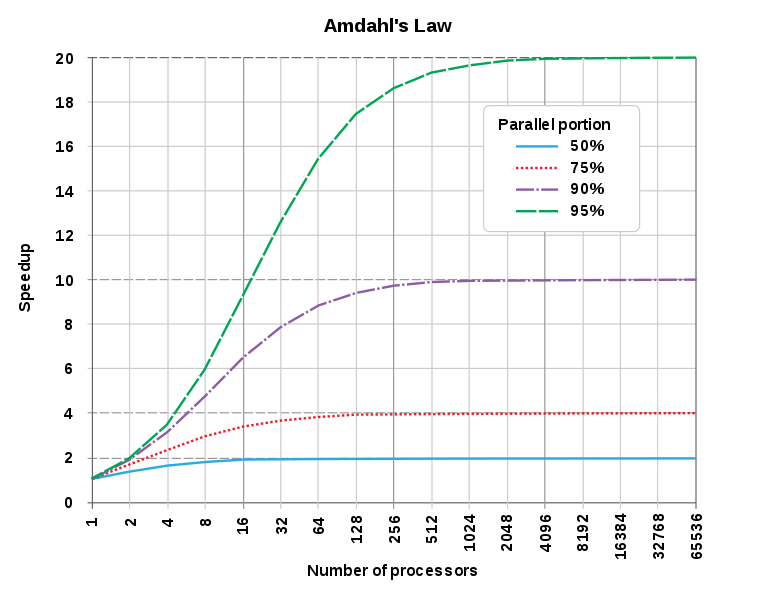
  Amdahl’s Law from Wikipedia

• Complexity - writing parallel code can be more complicated than writing serial code, especially in R because it does not natively implement parallel computing - you have to explicitly build it into your script.
• Dependencies - your computation may rely on the output from the first set of tasks to perform the second tasks. If you compute the problem in parallel fashion, the individual chunks do not communicate with one another.

• Parallel slowdown - parallel computing speeds up computations at a price. Once the problem is broken into separate threads, reading and writing data from the threads to memory or the hard drive takes time. Some tasks are not improved by spliting the process into parallel operations.

multidplyr

multidplyr is a work-in-progress package that implements parallel computing locally using dplyr. Rather than performing computations using a single core or processor, it spreads the computation across multiple cores. The basic sequence of steps is:

1. Call partition() to split the dataset across multiple cores. This makes a partitioned data frame, or a party df for short.
2. Each dplyr verb applied to a party df performs the operation independently on each core. It leaves each result on each core, and returns another party df.
3. When you’re done with the expensive operations that need to be done on each core, you call collect() to retrieve the data and bring it back to you local computer.

devtools::install_github("hadley/multidplyr")

library(multidplyr)
library(nycflights13)

flights1 <- partition(flights, flight)
flights2 <- summarize(flights1, dep_delay = mean(dep_delay, na.rm = TRUE))
flights3 <- collect(flights2)

flights2

## Source: party_df [3,844 x 2]
## Shards: 3 [1,237--1,304 rows]
## 
## # S3: party_df
##    flight  dep_delay
##     <int>      <dbl>
##  1      2 -0.5686275
##  2      3  3.6650794
##  3      4  7.5166240
##  4      6  8.5024155
##  5      8  6.9358974
##  6     10 24.3114754
##  7     11  6.8242991
##  8     12 28.2834646
##  9     15 10.2643080
## 10     19 10.0500000
## # ... with 3,834 more rows

system.time({
  flights %>% 
    partition() %>%
    summarise(mean(dep_delay, na.rm = TRUE)) %>% 
    collect()
})

##    user  system elapsed 
##   0.474   0.066   0.968

system.time({
  flights %>% 
    group_by() %>%
    summarise(mean(dep_delay, na.rm = TRUE))
})

##    user  system elapsed 
##   0.007   0.000   0.006

# split data into nests
gap_nested <- gapminder %>% 
  group_by(continent, country) %>% 
  nest()

# partition gap_nested across the cores
gap_nested_part <- gap_nested %>%
  partition(country)

# apply a linear model to each nested data frame
cluster_library(gap_nested_part, "purrr")

system.time({
  gap_nested_part %>% 
    mutate(fit = map(data, function(df) lm(lifeExp ~ year, data = df)))
})

##    user  system elapsed 
##   0.002   0.000   0.113

system.time({
  gap_nested %>% 
    mutate(fit = map(data, function(df) lm(lifeExp ~ year, data = df)))
})

##    user  system elapsed 
##   0.109   0.002   0.112