A dive into R Markdown
library(tidyverse)
library(rcfss)
set.seed(1234)
Reproducibility in scientific research
Reproducibility is “the idea that data analyses, and more generally, scientific claims, are published with their data and software code so that others may verify the findings and build upon them.”1 Scholars who implement reproducibility in their projects can quickly and easily reproduce the original results and trace back to determine how they were derived. This easily enables verification and replication, and allows the researcher to precisely replicate his or her analysis. This is extremely important when writing a paper, submiting it to a journal, then coming back months later for a revise and resubmit because you won’t remember how all the code/analysis works together when completing your revisions.
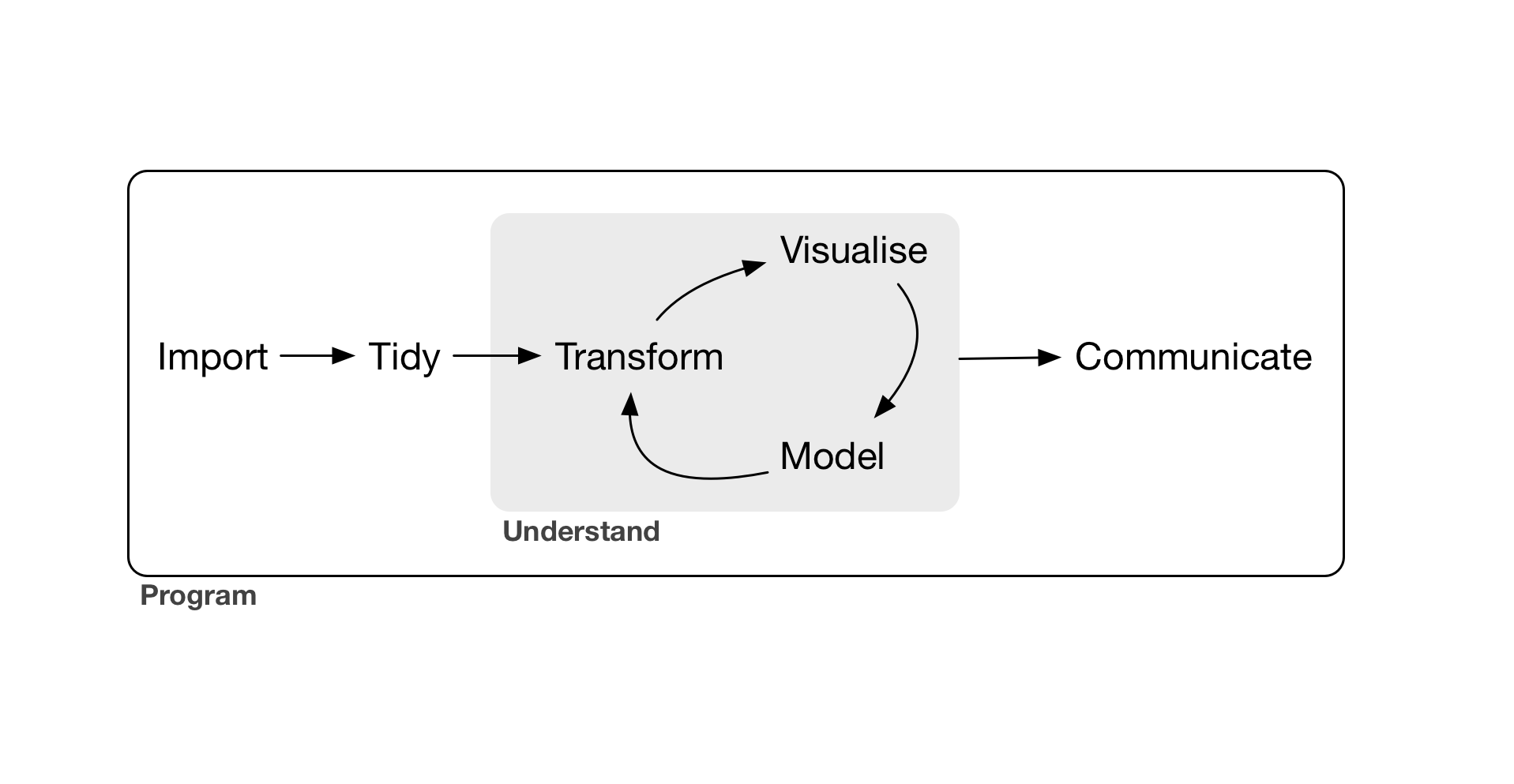
Reproducibility is also key for communicating findings with other researchers and decision makers; it allows them to verify your results, assess your assumptions, and understand how your answers were formed rather than solely relying on your claims. In the data science framework employed in R for Data Science, reproducibility is infused throughout the entire workflow.
R Markdown is one approach to ensuring reproducibility by providing a single cohesive authoring framework. It allows you to combine code, output, and analysis into a single document, are easily reproducible, and can be output to many different file formats. R Markdown is just one tool for enabling reproducibility. Another tool is Git for version control, which is crucial for collaboration and tracking changes to code and analysis.
Jupyter Notebooks
In the data science realm, another popular unified authoring framework is the Jupyter Notebook. The Jupyter Notebook (originally called iPython Notebook) is a web application that incorporates text, code, and output into a single document. Originally created for the Python programming language, Jupyter Notebooks are now multi-language and support over 40 programming languages, including R. You have probably seen or used them before.
There is nothing wrong with Jupyter Notebooks, but I prefer R Markdown because it is integrated into RStudio, arguably the best integrated development environment (IDE) for R. Furthermore, as you will see an R Markdown file is a plain-text file. This means the content of the file can be read by any text-editor, and is easily tracked by Git. Jupyter Notebooks are stored as JSON documents, a different and more complex file format. JSON is a useful format as we will see when we get to our modules on obtaining data from the web, but they are also much more difficult to track for revisions using Git. For this reason, in this course we will exclusively use R Markdown for reproducible documents.
R Markdown basics
An R Markdown file is a plain text file that uses the extension .Rmd:
---
title: "Gun deaths"
date: 2017-02-01
output: html_document
---
```{r setup, include = FALSE}
library(tidyverse)
library(rcfss)
youth <- gun_deaths %>%
filter(age <= 65)
```
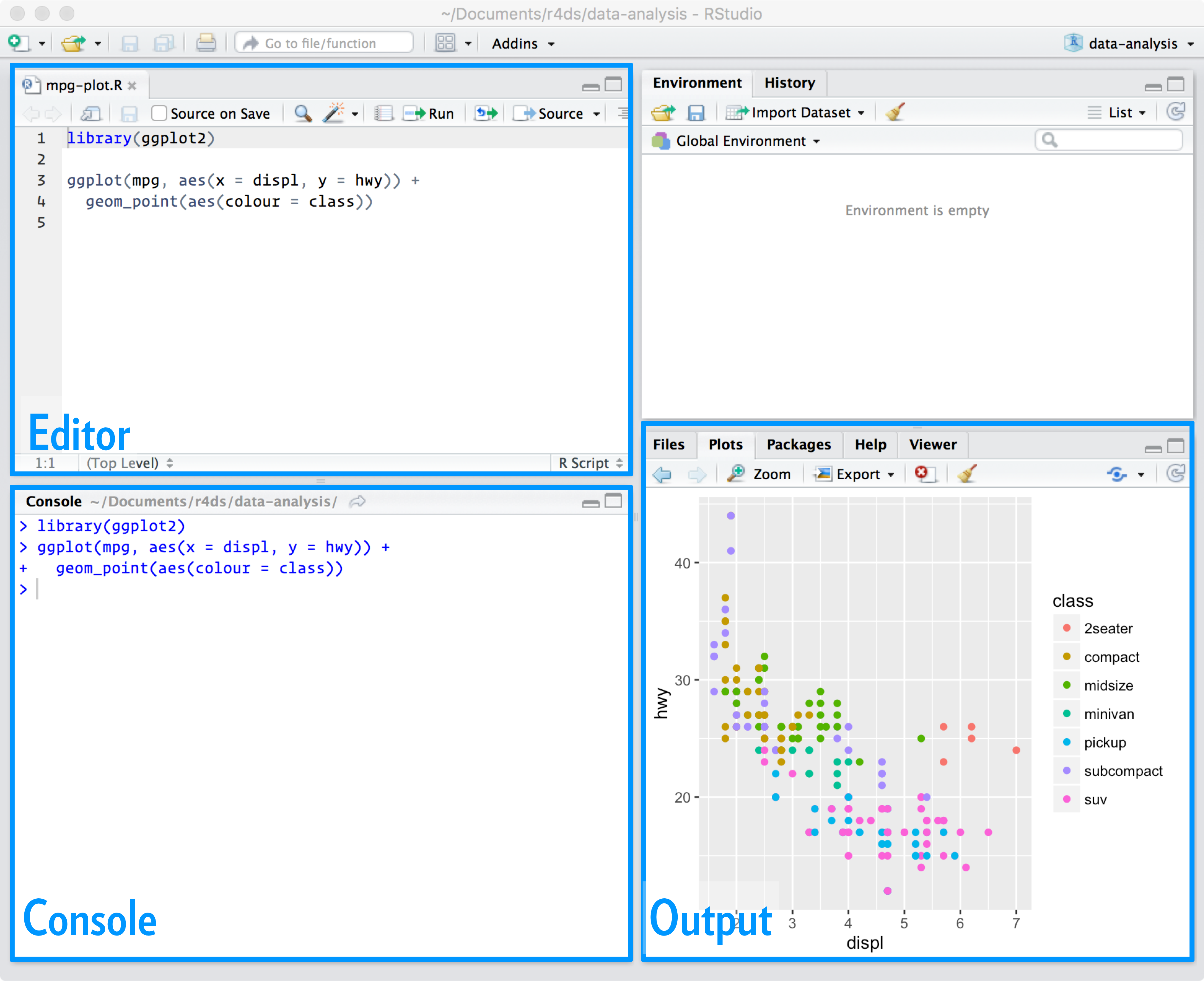
We have data about `r nrow(gun_deaths)` individuals killed by guns. Only `r nrow(gun_deaths) - nrow(youth)` are older than 65. The distribution of the remainder is shown below:
```{r youth-dist, echo = FALSE}
youth %>%
ggplot(aes(age)) +
geom_freqpoly(binwidth = 1)
```R Markdown documents contain 3 major components:
- A YAML header surrounded by
---s - Chunks of R code surounded by
``` - Text mixed with simple text formatting using the Markdown syntax
Code chunks are interspersed with text throughout the document. To complete the document, you “Knit” or “render” the document. Most of you proably knit the document by clicking the “Knit” button in the script editor panel. You can also do this programmatically from the console by running the command rmarkdown::render("example.Rmd").
When you knit the document you send your .Rmd file to knitr, a package for R that executes all the code chunks and creates a second markdown document (.md). That markdown document is then passed onto pandoc, a document rendering software program independent from R. Pandoc allows users to convert back and forth between many different document formats such as HTML, \(\LaTeX\), Microsoft Word, etc. By splitting the workflow up, you can convert your R Markdown document into a wide range of output formats.

Text formatting with Markdown
We have previously practiced formatting text using the Markdown syntax. I will not go into it further, but do note that there is a quick reference guide to Markdown built-in to RStudio. To access it, go to Help > Markdown Quick Reference.
Exercise
Copy and paste the contents of gun-deaths.Rmd (the file demonstrated above) and save it in a local R Markdown document. Check that you can run it, then add text after the frequency polygon that describes its most striking features.
Code chunks
Code chunks are where you store R code that will be executed. You can name a code chunk using the syntax ```{r name-here}. Naming chunks is a good practice to get into for several reasons. First, it makes navigating an R Markdown document using the drop-down code navigator in the bottom-left of the script editor easier since your chunks will have intuitive names. Second, it generates meaningful file names for any graphs created within the chunk, rather than unhelpful names such as unnamed-chunk-1.png. Finally, once you start caching your results (more on that below), using consistent names for chunks avoids having to repeat computationally intensive calculations.
Customizing chunks
Code chunks can be customized to adjust the output of the chunk. Some important and useful options are:
eval = FALSE- prevents code from being evaluated. I use this in my notes for class when I want to show how to write a specific function but don’t need to actually use it.include = FALSE- runs the code but doesn’t show the code or results in the final document. This is useful when you have setup code at the beginning of your document (loading packages, adjusting options, etc.) that may generate a lot of messages that are not really necessary to include in the final report.echo = FALSE- prevents code from showing in the final output, but does show the results of the code. Use this if you are writing a paper or document for someone who cares more about the substantive results and less about the programming used to obtain them.message = FALSEorwarning = FALSE- prevents messages or warnings from appearing in the final document.results = 'hide'- hides printed output.error = TRUE- causes the document to continue knitting and rendering even if the code generates a fatal error. I use this a lot when I want to intentionally demonstrate an error in class. If you’re debugging your code, you might want to use this option. However for the final version of your document, you probably do not want to allow errors to pass through unnoticed.
Caching
Remember the R Markdown workflow?
By default, every time you knit a document R starts completely fresh. None of the previous results are saved. If you have code chunks that run computationally intensive tasks, you might want to store these results to be more efficient and save time. If you use cache = TRUE, R will do exactly this. The output of the chunk will be saved to a specially named file on disk. If your .gitignore file is setup correctly, this cached file will not be tracked by Git. This is in fact preferable since the cached file could be hundreds of megabytes in size. Now, every time you knit the document the cached results will be used instead of running the code fresh.
Dependencies
This could be problematic when chunks rely on the output of previous chunks. Take this example from R for Data Science
```{r raw_data}
rawdata <- readr::read_csv("a_very_large_file.csv")
```

```{r processed_data, cache = TRUE}
processed_data <- rawdata %>%
  filter(!is.na(import_var)) %>%
  mutate(new_variable = complicated_transformation(x, y, z))
```
processed_data relies on the rawdata file created in the raw_data chunk. If you change your code in raw_data, processed_data will continue to rely on the older cached results. This means even if rawdata is altered, the cached results will continue to erroneously be used. To prevent this, use the dependson option to declare any chunks the cached chunk relies upon:
```{r processed_data, cache = TRUE, dependson = "raw_data"}
processed_data <- rawdata %>%
  filter(!is.na(import_var)) %>%
  mutate(new_variable = complicated_transformation(x, y, z))
```
Now if the code in the raw_data chunk is changed, processed_data will be run and the cache updated.
Global options
Rather than setting these options for each individual chunk, you can make them the default options for all chunks by using knitr::opts_chunk$set(). Just include this in a code chunk (typically in the first code chunk in the document). So for example,
knitr::opts_chunk$set(
  echo = FALSE
)
hides the code by default in all code chunks. To override this new default, you can still declare echo = TRUE for individual chunks.
Inline code
Until now, you have only run code in a specially designated chunk. However you can also run R code in-line by using the `r ` syntax. For example, look at the text from the example document earlier:
We have data about
`r nrow(gun_deaths)`individuals killed by guns. Only`r nrow(gun_deaths) - nrow(youth)`are older than 65. The distribution of the remainder is shown below:
When you knit the document, the R code is executed:
We have data about 100798 individuals killed by guns. Only 15687 are older than 65. The distribution of the remainder is shown below:
Exercise: practice chunk options
Add a section that explores how gun deaths vary by race.
- Assume you’re writing a report for someone who doesn’t know R, and instead of setting
echo = FALSEon each chunk, set a global option. - Enable caching as a global option and render the document. Look at the file structure for the cache. Now render the document again. Does it run faster? Modify some code in one of the chunks? What happens now?
- Test out some of the other chunk options. Which do you find most useful? In what context would you use them?
YAML header
Yet Another Markup Language, or YAML (rhymes with camel) is a standardized format for storing hierarchical data in a human-readable syntax. The YAML header controls how rmarkdown renders your .Rmd file. A YAML header is a section of key: value pairs surrounded by --- marks.
---
title: "Gun deaths"
author: "Benjamin Soltoff"
date: 2017-02-01
output: html_document
---
The most important option is output, as this determines the final document format. However there are other common options such as providing a title and author for your document and specifying the date of publication.
Output formats
HTML document
For your homework assignments, we have used github_document to generate a Markdown document. However there are other document formats that are more commonly used.
---
title: "Untitled"
author: "Benjamin Soltoff"
date: "February 1, 2017"
output: html_document
---
output: html_document produces an HTML document. The nice feature of this document is that all images are embedded in the HTML file itself, so you can email just the .html file to someone and they will be able to open and read it.
Table of contents
Each output format has various options to customize the appearance of the final document. One option for HTML documents is to add a table of contents through the toc option. To add any option for an output format, just add it in a hierarchical format like this:
---
title: "Untitled"
author: "Benjamin Soltoff"
date: "February 1, 2017"
output:
  html_document:
    toc: true
    toc_depth: 2
You can explicitly set the number of levels included in the table of contents with toc_depth (the default is 3).
Appearance and style
There are several options that control the visual appearance of HTML documents.
themespecifies the Bootstrap theme to use for the page (themes are drawn from the Bootswatch theme library). Valid themes include"default","cerulean","journal","flatly","readable","spacelab","united","cosmo","lumen","paper","sandstone","simplex", and"yeti".highlightspecifies the syntax highlighting style for code chunks. Supported styles include"default","tango","pygments","kate","monochrome","espresso","zenburn","haddock", and"textmate".
This course site uses the R Markdown Websites format to render multiple
.Rmddocuments in a single website. It uses thereadabletheme andpygmentshighlighting.
---
title: "Untitled"
author: "Benjamin Soltoff"
date: "February 1, 2017"
output:
  html_document:
    theme: readable
    highlight: pygments
---
Code folding
Sometimes when knitting an R Markdown document you want to include your R source code (echo = TRUE) but you may want to include it but not make it visible by default. The code_folding: hide options allows you to include your R code but hide it. Users can then decide whether or not they want to see specific chunks or all chunks in the document. This strikes a good balance between readability and reproducibility.
---
title: "Untitled"
author: "Benjamin Soltoff"
date: "February 1, 2017"
output:
  html_document:
    code_folding: hide
---
Keeping Markdown
When knitr processes your .Rmd document, it creates a Markdown (.md) file that is subsequently deleted. If you want to keep a copy of the Markdown file use the keep_md option:
---
title: "Untitled"
author: "Benjamin Soltoff"
date: "February 1, 2017"
output:
  html_document:
    keep_md: true
---
Exercise: test HTML options
Use the gun-deaths.Rmd file you saved on your computer and test some of the document options outlined above. There are far more customization options than I outlined above. Read the help file for HTML documents to learn about more of the available options.
PDF document
pdf_document converts the .Rmd file to a \(\LaTeX\) file which is used to generate a PDF.
---
title: "Gun deaths"
date: 2017-02-01
output: pdf_document
---
You do need to have a full installation of TeX on your computer to generate PDF output. However the nice thing is that because it uses the \(\LaTeX\) rendering engine, you can use raw \(\LaTeX\) code in your .Rmd file (if you know how to use it).
Table of contents
Many options for HTML documents also work for PDFs. For instance, you create a table of contents the same way:
---
title: "Untitled"
author: "Benjamin Soltoff"
date: "February 1, 2017"
output:
  pdf_document:
    toc: true
    toc_depth: 2
Syntax highlighting
You cannot customize the theme of a pdf_document (at least not in the same way as HTML files), but you can still customize the syntax highlighting.
---
title: "Untitled"
author: "Benjamin Soltoff"
date: "February 1, 2017"
output:
  pdf_document:
    highlight: pygments
---
\(\LaTeX\) options
You can also directly control options in the \(\LaTeX\) template itself via the YAML options. Note that these options are passed as top-level YAML metadata, not underneath the output section:
---
title: "Untitled"
author: "Benjamin Soltoff"
date: "February 1, 2017"
output: pdf_document
fontsize: 11pt
geometry: margin=1in
---
Keep intermediate TeX
R Markdown documents are converted first to a .tex file, and then use the \(\LaTeX\) engine to convert to PDF. To keep the .tex file, use the keep_tex option:
---
title: "Untitled"
author: "Benjamin Soltoff"
date: "February 1, 2017"
output:
  pdf_document:
    keep_tex: true
---
Exercise: test PDF options
Use the gun-deaths.Rmd file you saved on your computer and test some of the PDF document options outlined above. Be sure to first change the output format to pdf_document. There are far more customization options than I outlined above. Read the help file for PDF documents to learn about more of the available options.
Presentations
You can use R Markdown not only to generate full documents, but also slide presentations. There are four major presentation formats:
- ioslides - HTML presentation with ioslides
- reveal.js - HTML presentation with reveal.js
- Slidy - HTML presentation with W3C Slidy
- Beamer - PDF presentation with \(\LaTeX\) Beamer
Each as their own strengths and weaknesses. ioslides and Slidy are probably the easiest to use initially, but are more difficult to customize. reveal.js is more complex, but allows for more customization (this is the format I use for my slides in this class). Beamer is the only presentation format that creates a PDF document and is probably a smoother transition for those already used to Beamer.
Exercise: build a presentation
Choose one of the presentation formats and convert gun-deaths.Rmd into a slide presentation. Save this new document as gun-deaths-slides.Rmd. Test out some of the associated options for your chosen presentation format.
Multiple formats
You can even render your document into multiple output formats by supplying a list of formats:
output:
  html_document:
    toc: true
    toc_float: true
  pdf_document: default
If you don’t want to change any of the default options for a format, use the default option. You cannot specify multiple formats like this:
output:
  html_document:
    toc: true
    toc_float: true
  pdf_document
You must assign some value to the second output format, hence the use of default.
Rendering multiple outputs programmatically
When rendering multiple output formats, you cannot just click the “Knit” button. Doing so will only render the first output format listed in the YAML. To render all output formats, you need to programmatically render the document using rmarkdown::render("my-document.Rmd", output_format = "all"). Type ?render in the console to look up the help file for render() and see the different arguments the function can accept.
Exercise: render in multiple formats
Render gun-deaths.Rmd as both an HTML document and a PDF document. If you do not have \(\LaTeX\) installed on your computer, render gun-deaths.Rmd as both an HTML document and a Word document. And at some point install \(\LaTeX\) on your computer so you can create PDF documents.
R scripts
So far we’ve done a lot of our work in R Markdown documents, knitting together code chunks, output, and Markdown text. However we don’t have to use R Markdown documents for all our work. In many instances, using a script might be preferable.
What is a script?
A script is a plain-text file with a .R file extension. It contains R code. You can add comments using the # symbol. For example, gun-deaths.R would look something like this:
# gun-deaths.R
# 2017-02-01
# Examine the distribution of age of victims in gun_deaths


# load packages
library(tidyverse)
library(rcfss)

# filter data for under 65
youth <- gun_deaths %>%
  filter(age <= 65)

# number of individuals under 65 killed
nrow(gun_deaths) - nrow(youth)

# graph the distribution of youth
youth %>%
  ggplot(aes(age)) +
  geom_freqpoly(binwidth = 1)
You edit scripts in the editor panel in R Studio.
When to use a script?
Scripts are much easier to troubleshoot than R Markdown documents because your code is not split across chunks and you can run everything interactively. When you first begin a project, you may find it useful to use scripts initially to build and debug code, then convert it to an R Markdown document once you begin the substantive analysis and writeup. Or you may use a mix of scripts and R Markdown documents depending on the size and complexity of your project. For instance, you could use a reproducible pipeline which uses a sequence of R scripts to download, import, and transform your data, then use an R Markdown document to produce a final report.
Check out this example for how one could use a pipeline in this fashion.
In this class while the final product is generally submitted as an R Markdown document, it is fine to do your initial work in an R script. If you find it easier to write and debug code there, then use that approach. Or if you prefer the R Markdown lab notebook workflow, then use that. By this point you have enough competence in R to decide what works for you and what does not. Find what works best for you and do that.
Running scripts interactively
You can run sections of your script by highlighting the appropriate code and typing Cmd/Ctrl + Enter. You can also run code expression-by-expression by placing your cursor at the appropriate expression in the script and typing Cmd/Ctrl + Enter. To run the entire script at once, type Cmd/Ctrl + Shift + S or press “Run” at the top of the script editor panel.
Running scripts programmatically
To run a script saved on your computer, use the source() function in the console. As in source("gun-deaths.R"). You can also include this command in a second script. By doing this you can execute a sequence of related scripts all in order, rather than having to run each one manually in the console. See runfile.R from the pipeline-example repo to see this in action. Remember that R scripts (.R) are executed via the source() function, whereas R Markdown files (.Rmd) are executed via the rmarkdown::render() function.
Want to create a report from an R script? Just call
rmarkdown::render("gun-deaths.R")to author an R Markdown document based on the R script. It will never be as fully featured as if you originally wrote it in an R Markdown document, but can sometimes be handy. Read this overview for more details on this procedure.
Running scripts via the shell
You can also run scripts directly from the shell using Rscript:
Rscript gun-deaths.RTo render an R Markdown document from the shell, we use the syntax:
Rscript -e "rmarkdown::render('gun-deaths.Rmd')"This creates a temporary R script which contains the single command rmarkdown::render('gun-deaths.Rmd') and executes it via Rscript.
Exercise: execute R scripts
- Convert your revised
gun-deaths.Rmddocument into an R script calledgun-deaths.R. - Practice running segments of code interactively
- Run the entire script via the
source()function - Use the shell to run
gun-deaths.R
Session Info
devtools::session_info()## Session info -------------------------------------------------------------## setting value
## version R version 3.4.1 (2017-06-30)
## system x86_64, darwin15.6.0
## ui X11
## language (EN)
## collate en_US.UTF-8
## tz America/Chicago
## date 2017-08-08## Packages -----------------------------------------------------------------## package * version date source
## assertthat 0.2.0 2017-04-11 CRAN (R 3.4.0)
## backports 1.1.0 2017-05-22 CRAN (R 3.4.0)
## base * 3.4.1 2017-07-07 local
## bindr 0.1 2016-11-13 CRAN (R 3.4.0)
## bindrcpp 0.2 2017-06-17 CRAN (R 3.4.0)
## boxes 0.0.0.9000 2017-07-19 Github (r-pkgs/boxes@03098dc)
## broom 0.4.2 2017-02-13 CRAN (R 3.4.0)
## cellranger 1.1.0 2016-07-27 CRAN (R 3.4.0)
## clisymbols 1.2.0 2017-05-21 cran (@1.2.0)
## colorspace 1.3-2 2016-12-14 CRAN (R 3.4.0)
## compiler 3.4.1 2017-07-07 local
## crayon 1.3.2.9000 2017-07-19 Github (gaborcsardi/crayon@750190f)
## datasets * 3.4.1 2017-07-07 local
## devtools 1.13.2 2017-06-02 CRAN (R 3.4.0)
## digest 0.6.12 2017-01-27 CRAN (R 3.4.0)
## dplyr * 0.7.2 2017-07-20 CRAN (R 3.4.1)
## evaluate 0.10.1 2017-06-24 CRAN (R 3.4.1)
## forcats * 0.2.0 2017-01-23 CRAN (R 3.4.0)
## foreign 0.8-69 2017-06-22 CRAN (R 3.4.1)
## ggplot2 * 2.2.1 2016-12-30 CRAN (R 3.4.0)
## glue 1.1.1 2017-06-21 CRAN (R 3.4.1)
## graphics * 3.4.1 2017-07-07 local
## grDevices * 3.4.1 2017-07-07 local
## grid 3.4.1 2017-07-07 local
## gtable 0.2.0 2016-02-26 CRAN (R 3.4.0)
## haven 1.1.0 2017-07-09 CRAN (R 3.4.1)
## hms 0.3 2016-11-22 CRAN (R 3.4.0)
## htmltools 0.3.6 2017-04-28 CRAN (R 3.4.0)
## httr 1.2.1 2016-07-03 CRAN (R 3.4.0)
## jsonlite 1.5 2017-06-01 CRAN (R 3.4.0)
## knitr 1.16 2017-05-18 CRAN (R 3.4.0)
## lattice 0.20-35 2017-03-25 CRAN (R 3.4.1)
## lazyeval 0.2.0 2016-06-12 CRAN (R 3.4.0)
## lubridate 1.6.0 2016-09-13 CRAN (R 3.4.0)
## magrittr 1.5 2014-11-22 CRAN (R 3.4.0)
## memoise 1.1.0 2017-04-21 CRAN (R 3.4.0)
## methods * 3.4.1 2017-07-07 local
## mnormt 1.5-5 2016-10-15 CRAN (R 3.4.0)
## modelr 0.1.1 2017-07-24 CRAN (R 3.4.1)
## munsell 0.4.3 2016-02-13 CRAN (R 3.4.0)
## nlme 3.1-131 2017-02-06 CRAN (R 3.4.1)
## parallel 3.4.1 2017-07-07 local
## pkgconfig 2.0.1 2017-03-21 CRAN (R 3.4.0)
## plyr 1.8.4 2016-06-08 CRAN (R 3.4.0)
## psych 1.7.5 2017-05-03 CRAN (R 3.4.1)
## purrr * 0.2.2.2 2017-05-11 CRAN (R 3.4.0)
## R6 2.2.2 2017-06-17 CRAN (R 3.4.0)
## rcfss * 0.1.5 2017-07-31 local
## Rcpp 0.12.12 2017-07-15 CRAN (R 3.4.1)
## readr * 1.1.1 2017-05-16 CRAN (R 3.4.0)
## readxl 1.0.0 2017-04-18 CRAN (R 3.4.0)
## reshape2 1.4.2 2016-10-22 CRAN (R 3.4.0)
## rlang 0.1.1 2017-05-18 CRAN (R 3.4.0)
## rmarkdown 1.6 2017-06-15 CRAN (R 3.4.0)
## rprojroot 1.2 2017-01-16 CRAN (R 3.4.0)
## rstudioapi 0.6 2016-06-27 CRAN (R 3.4.0)
## rvest 0.3.2 2016-06-17 CRAN (R 3.4.0)
## scales 0.4.1 2016-11-09 CRAN (R 3.4.0)
## stats * 3.4.1 2017-07-07 local
## stringi 1.1.5 2017-04-07 CRAN (R 3.4.0)
## stringr * 1.2.0 2017-02-18 CRAN (R 3.4.0)
## tibble * 1.3.3 2017-05-28 CRAN (R 3.4.0)
## tidyr * 0.6.3 2017-05-15 CRAN (R 3.4.0)
## tidyverse * 1.1.1.9000 2017-07-19 Github (tidyverse/tidyverse@a028619)
## tools 3.4.1 2017-07-07 local
## utils * 3.4.1 2017-07-07 local
## withr 2.0.0 2017-07-28 CRAN (R 3.4.1)
## xml2 1.1.1 2017-01-24 CRAN (R 3.4.0)
## yaml 2.1.14 2016-11-12 CRAN (R 3.4.0)This work is licensed under the CC BY-NC 4.0 Creative Commons License.