Vectors
library(tidyverse)
set.seed(1234)
So far the only type of data object in R you have encountered is a data.frame (or the tidyverse variant tibble). At its core though, the primary method of data storage in R is the vector. So far we have only encountered vectors as components of a data frame; data frames are built from vectors. There are a few different types of vectors: logical, numeric, and character. But now we want to understand more precisely how these data objects are structured and related to one another.
Types of vectors
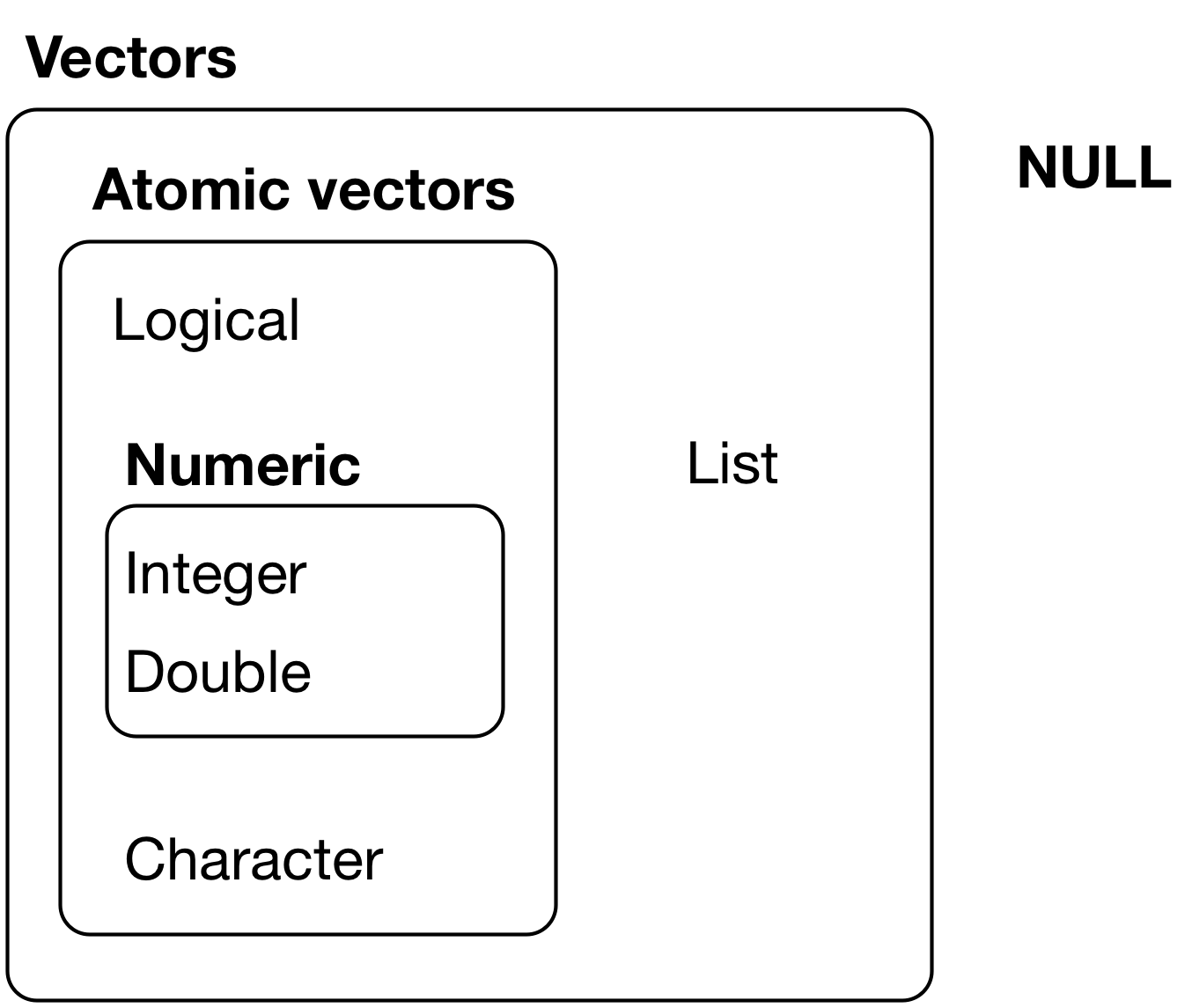
Figure 20.1 from R for Data Science
There are two categories of vectors:
- Atomic vectors - these are the types previously covered, including logical, integer, double, and character.
- Lists - there are new and we will cover them later in this module. Lists are distinct from atomic vectors because lists can contain other lists.
Atomic vectors are homogenous - that is, all elements of the vector must be the same type. Lists can be hetergenous and contain multiple types of elements. NULL is the counterpart to NA. While NA represents the absence of a value, NULL represents the absence of a vector.
Atomic vectors
Logical vectors
Logical vectors take on one of three possible values:
TRUEFALSENA(missing value)
parse_logical(c(TRUE, TRUE, FALSE, TRUE, NA))## [1] TRUE TRUE FALSE TRUE NAWhenever you filter a data frame, R is (in the background) creating a vector of
TRUEandFALSE- whenever the condition isTRUE, keep the row, otherwise exclude it.
Numeric vectors
Numeric vectors contain numbers (duh!). They can be stored as integers (whole numbers) or doubles (numbers with decimal points). In practice, you rarely need to concern yourself with this difference, but just know that they are different but related things.
parse_integer(c(1, 5, 3, 4, 12423))## [1] 1 5 3 4 12423parse_double(c(4.2, 4, 6, 53.2))## [1] 4.2 4.0 6.0 53.2Doubles can store both whole numbers and numbers with decimal points.
Character vectors
Character vectors contain strings, which are typically text but could also be dates or any other combination of characters.
parse_character(c("Goodnight Moon", "Runaway Bunny", "Big Red Barn"))## [1] "Goodnight Moon" "Runaway Bunny" "Big Red Barn"Using atomic vectors
Be sure to read “Using atomic vectors” for more detail on how to use and interact with atomic vectors. I have no desire to rehash everything Hadley already wrote, but here are a couple things about atomic vectors I want to reemphasize.
Scalars
Scalars are a single number; vectors are a set of multiple values. In R, scalars are merely a vector of length 1. So when you try to perform arithmetic or other types of functions on a vector, it will recycle the scalar value.
(x <- sample(10))## [1] 2 6 5 8 9 4 1 7 10 3x + c(100, 100, 100, 100, 100, 100, 100, 100, 100, 100)## [1] 102 106 105 108 109 104 101 107 110 103x + 100## [1] 102 106 105 108 109 104 101 107 110 103This is why you don’t need to write an iterative operation when performing these basic operations - R automatically converts it for you.
Sometimes this isn’t so great, because R will also recycle vectors if the lengths are not equal:
# create a sequence of numbers between 1 and 10
(x1 <- seq(from = 1, to = 2))
## [1] 1 2(x2 <- seq(from = 1, to = 10))## [1] 1 2 3 4 5 6 7 8 9 10# add together two sequences of numbers
x1 + x2## [1] 2 4 4 6 6 8 8 10 10 12Did you really mean to recycle 1:2 five times, or was this actually an error? tidyverse functions will only allow you to implicitly recycle scalars, otherwise it will throw an error and you’ll have to manually recycle shorter vectors.
Subsetting
To filter a vector, we cannot use filter() because that only works for filtering rows in a tibble. [ is the subsetting function for vectors. It is used like x[a].
Subset with a numeric vector containing integers
(x <- c("one", "two", "three", "four", "five"))## [1] "one" "two" "three" "four" "five"Subset with positive integers keeps the corresponding elements:
x[c(3, 2, 5)]## [1] "three" "two" "five"Negative values drop the corresponding elements:
x[c(-1, -3, -5)]## [1] "two" "four"You cannot mix positive and negative values:
x[c(-1, 1)]## Error in x[c(-1, 1)]: only 0's may be mixed with negative subscriptsSubset with a logical vector
Subsetting with a logical vector keeps all values corresponding to a TRUE value.
(x <- c(10, 3, NA, 5, 8, 1, NA))## [1] 10 3 NA 5 8 1 NA# All non-missing values of x
!is.na(x)## [1] TRUE TRUE FALSE TRUE TRUE TRUE FALSEx[!is.na(x)]## [1] 10 3 5 8 1# All even (or missing!) values of x
x[x %% 2 == 0]## [1] 10 NA 8 NAExercise: subset the vector
(x <- seq(from = 1, to = 10))## [1] 1 2 3 4 5 6 7 8 9 10Create the sequence above in your R session. Write commands to subset the vector in the following ways:
Keep the first through fourth elements, plus the seventh element.
Click for the solution
x[c(1, 2, 3, 4, 7)]## [1] 1 2 3 4 7# use a sequence shortcut x[c(seq(1, 4), 7)]## [1] 1 2 3 4 7Keep the first through eighth elements, plus the tenth element.
Click for the solution
# long way
x[c(1, 2, 3, 4, 5, 6, 7, 8, 10)]
## [1] 1 2 3 4 5 6 7 8 10# sequence shortcut x[c(seq(1, 8), 10)]## [1] 1 2 3 4 5 6 7 8 10# negative indexing x[c(-9)]## [1] 1 2 3 4 5 6 7 8 10Keep all elements with values greater than five.
Click for the solution
# get the index for which values in x are greater than 5
x > 5
## [1] FALSE FALSE FALSE FALSE FALSE TRUE TRUE TRUE TRUE TRUEx[x > 5]## [1] 6 7 8 9 10Keep all elements evenly divisible by three.
Click for the solution
x[x %% 3 == 0]## [1] 3 6 9
Lists
Lists are an entirely different type of vector.
x <- list(1, 2, 3)
x
## [[1]]
## [1] 1
##
## [[2]]
## [1] 2
##
## [[3]]
## [1] 3Use str() to view the structure of the list.
str(x)## List of 3
## $ : num 1
## $ : num 2
## $ : num 3x_named <- list(a = 1, b = 2, c = 3)
str(x_named)## List of 3
## $ a: num 1
## $ b: num 2
## $ c: num 3If you are running RStudio 1.1 or above, you can also use the object explorer to interactively examine the structure of objects.
Unlike the other atomic vectors, lists are recursive. This means they can:
Store a mix of objects.
y <- list("a", 1L, 1.5, TRUE)
str(y)
## List of 4 ## $ : chr "a" ## $ : int 1 ## $ : num 1.5 ## $ : logi TRUEContain other lists.
z <- list(list(1, 2), list(3, 4))
str(z)
## List of 2 ## $ :List of 2 ## ..$ : num 1 ## ..$ : num 2 ## $ :List of 2 ## ..$ : num 3 ## ..$ : num 4It isn’t immediately apparent why you would want to do this, but in later units we will discover the value of lists as many packages for R store non-tidy data as lists.
You’ve already worked with lists without even knowing it. Data frames and tibbles are a type of a list. Notice that you can store a data frame with a mix of column types.
str(diamonds)## Classes 'tbl_df', 'tbl' and 'data.frame': 53940 obs. of 10 variables:
## $ carat : num 0.23 0.21 0.23 0.29 0.31 0.24 0.24 0.26 0.22 0.23 ...
## $ cut : Ord.factor w/ 5 levels "Fair"<"Good"<..: 5 4 2 4 2 3 3 3 1 3 ...
## $ color : Ord.factor w/ 7 levels "D"<"E"<"F"<"G"<..: 2 2 2 6 7 7 6 5 2 5 ...
## $ clarity: Ord.factor w/ 8 levels "I1"<"SI2"<"SI1"<..: 2 3 5 4 2 6 7 3 4 5 ...
## $ depth : num 61.5 59.8 56.9 62.4 63.3 62.8 62.3 61.9 65.1 59.4 ...
## $ table : num 55 61 65 58 58 57 57 55 61 61 ...
## $ price : int 326 326 327 334 335 336 336 337 337 338 ...
## $ x : num 3.95 3.89 4.05 4.2 4.34 3.94 3.95 4.07 3.87 4 ...
## $ y : num 3.98 3.84 4.07 4.23 4.35 3.96 3.98 4.11 3.78 4.05 ...
## $ z : num 2.43 2.31 2.31 2.63 2.75 2.48 2.47 2.53 2.49 2.39 ...How to subset lists
Sometimes lists (especially deeply-nested lists) can be confusing to view and manipulate. Take the example from R for Data Science:
a <- list(a = 1:3, b = "a string", c = pi, d = list(-1, -5))
str(a)
## List of 4
## $ a: int [1:3] 1 2 3
## $ b: chr "a string"
## $ c: num 3.14
## $ d:List of 2
## ..$ : num -1
## ..$ : num -5[extracts a sub-list. The result will always be a list.str(a[1:2])## List of 2 ## $ a: int [1:3] 1 2 3 ## $ b: chr "a string"str(a[4])## List of 1 ## $ d:List of 2 ## ..$ : num -1 ## ..$ : num -5[[extracts a single component from a list and removes a level of hierarchy.str(a[[1]])## int [1:3] 1 2 3str(a[[4]])## List of 2 ## $ : num -1 ## $ : num -5$can be used to extract named elements of a list.a$a## [1] 1 2 3a[['a']]## [1] 1 2 3a[["a"]]## [1] 1 2 3
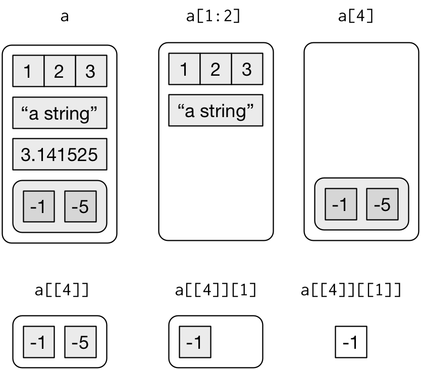
Figure 20.2 from R for Data Science
Still confused about list subsetting? Review the pepper shaker.
Exercise: subset a list
a <- list(a = 1:3, b = "a string", c = pi, d = list(-1, -5))
str(a)
## List of 4
## $ a: int [1:3] 1 2 3
## $ b: chr "a string"
## $ c: num 3.14
## $ d:List of 2
## ..$ : num -1
## ..$ : num -5Create the list above in your R session. Write commands to subset the list in the following ways:
Subset
a. The result should be an atomic vector.Click for the solution
# use the index value
a[[1]]
## [1] 1 2 3# use the element name a$a## [1] 1 2 3a[["a"]]## [1] 1 2 3Subset
pi. The results should be a new list.Click for the solution
# correct method
str(a["c"])
## List of 1 ## $ c: num 3.14# incorrect method to produce another list # the result is a scalar str(a$c)## num 3.14Subset the first and third elements from
a.Click for the solution
a[c(1, 3)]## $a ## [1] 1 2 3 ## ## $c ## [1] 3.141593a[c("a", "c")]## $a ## [1] 1 2 3 ## ## $c ## [1] 3.141593
Session Info
devtools::session_info()## Session info -------------------------------------------------------------## setting value
## version R version 3.4.3 (2017-11-30)
## system x86_64, darwin15.6.0
## ui X11
## language (EN)
## collate en_US.UTF-8
## tz America/Chicago
## date 2018-04-18## Packages -----------------------------------------------------------------## package * version date source
## assertthat 0.2.0 2017-04-11 CRAN (R 3.4.0)
## backports 1.1.2 2017-12-13 CRAN (R 3.4.3)
## base * 3.4.3 2017-12-07 local
## bindr 0.1.1 2018-03-13 CRAN (R 3.4.3)
## bindrcpp 0.2.2.9000 2018-04-08 Github (krlmlr/bindrcpp@bd5ae73)
## broom 0.4.4 2018-03-29 CRAN (R 3.4.3)
## cellranger 1.1.0 2016-07-27 CRAN (R 3.4.0)
## cli 1.0.0 2017-11-05 CRAN (R 3.4.2)
## colorspace 1.3-2 2016-12-14 CRAN (R 3.4.0)
## compiler 3.4.3 2017-12-07 local
## crayon 1.3.4 2017-10-03 Github (gaborcsardi/crayon@b5221ab)
## datasets * 3.4.3 2017-12-07 local
## devtools 1.13.5 2018-02-18 CRAN (R 3.4.3)
## digest 0.6.15 2018-01-28 CRAN (R 3.4.3)
## dplyr * 0.7.4.9003 2018-04-08 Github (tidyverse/dplyr@b7aaa95)
## evaluate 0.10.1 2017-06-24 CRAN (R 3.4.1)
## forcats * 0.3.0 2018-02-19 CRAN (R 3.4.3)
## foreign 0.8-69 2017-06-22 CRAN (R 3.4.3)
## ggplot2 * 2.2.1.9000 2018-04-10 Github (tidyverse/ggplot2@3c9c504)
## glue 1.2.0 2017-10-29 CRAN (R 3.4.2)
## graphics * 3.4.3 2017-12-07 local
## grDevices * 3.4.3 2017-12-07 local
## grid 3.4.3 2017-12-07 local
## gtable 0.2.0 2016-02-26 CRAN (R 3.4.0)
## haven 1.1.1 2018-01-18 CRAN (R 3.4.3)
## hms 0.4.2 2018-03-10 CRAN (R 3.4.3)
## htmltools 0.3.6 2017-04-28 CRAN (R 3.4.0)
## httr 1.3.1 2017-08-20 CRAN (R 3.4.1)
## jsonlite 1.5 2017-06-01 CRAN (R 3.4.0)
## knitr 1.20 2018-02-20 CRAN (R 3.4.3)
## lattice 0.20-35 2017-03-25 CRAN (R 3.4.3)
## lazyeval 0.2.1 2017-10-29 CRAN (R 3.4.2)
## lubridate 1.7.4 2018-04-11 CRAN (R 3.4.3)
## magrittr 1.5 2014-11-22 CRAN (R 3.4.0)
## memoise 1.1.0 2017-04-21 CRAN (R 3.4.0)
## methods * 3.4.3 2017-12-07 local
## mnormt 1.5-5 2016-10-15 CRAN (R 3.4.0)
## modelr 0.1.1 2017-08-10 local
## munsell 0.4.3 2016-02-13 CRAN (R 3.4.0)
## nlme 3.1-137 2018-04-07 CRAN (R 3.4.4)
## parallel 3.4.3 2017-12-07 local
## pillar 1.2.1 2018-02-27 CRAN (R 3.4.3)
## pkgconfig 2.0.1 2017-03-21 CRAN (R 3.4.0)
## plyr 1.8.4 2016-06-08 CRAN (R 3.4.0)
## psych 1.8.3.3 2018-03-30 CRAN (R 3.4.4)
## purrr * 0.2.4 2017-10-18 CRAN (R 3.4.2)
## R6 2.2.2 2017-06-17 CRAN (R 3.4.0)
## Rcpp 0.12.16 2018-03-13 CRAN (R 3.4.4)
## readr * 1.1.1 2017-05-16 CRAN (R 3.4.0)
## readxl 1.0.0 2017-04-18 CRAN (R 3.4.0)
## reshape2 1.4.3 2017-12-11 CRAN (R 3.4.3)
## rlang 0.2.0.9001 2018-04-10 Github (r-lib/rlang@70d2d40)
## rmarkdown 1.9 2018-03-01 CRAN (R 3.4.3)
## rprojroot 1.3-2 2018-01-03 CRAN (R 3.4.3)
## rstudioapi 0.7 2017-09-07 CRAN (R 3.4.1)
## rvest 0.3.2 2016-06-17 CRAN (R 3.4.0)
## scales 0.5.0.9000 2018-04-10 Github (hadley/scales@d767915)
## stats * 3.4.3 2017-12-07 local
## stringi 1.1.7 2018-03-12 CRAN (R 3.4.3)
## stringr * 1.3.0 2018-02-19 CRAN (R 3.4.3)
## tibble * 1.4.2 2018-01-22 CRAN (R 3.4.3)
## tidyr * 0.8.0 2018-01-29 CRAN (R 3.4.3)
## tidyselect 0.2.4 2018-02-26 CRAN (R 3.4.3)
## tidyverse * 1.2.1 2017-11-14 CRAN (R 3.4.2)
## tools 3.4.3 2017-12-07 local
## utils * 3.4.3 2017-12-07 local
## withr 2.1.2 2018-04-10 Github (jimhester/withr@79d7b0d)
## xml2 1.2.0 2018-01-24 CRAN (R 3.4.3)
## yaml 2.1.18 2018-03-08 CRAN (R 3.4.4)This work is licensed under the CC BY-NC 4.0 Creative Commons License.