Statistical learning: resampling methods
library(tidyverse)
library(modelr)
library(broom)
set.seed(1234)

theme_set(theme_minimal())
Resampling methods
Resampling methods are essential to test and evaluate statistical models. Because you likely do not have the resources or capabilities to repeatedly sample from your population of interest, instead you can repeatedly draw from your original sample to obtain additional information about your model. For instance, you could repeatedly draw samples from your data, estimate a linear regression model on each sample, and then examine how the estimated model differs across each sample. This allows you to assess the variability and stability of your model in a way not possible if you can only fit the model once.
Validation set
One issue with using the same data to both fit and evaluate our model is that we will bias our model towards fitting the data that we have. We may fit our function to create the results we expect or desire, rather than the “true” function. Instead, we can split our data into distinct training and test sets. The training set can be used repeatedly to explore or train different models. Once we have a stable model, we can apply it to the test set of held-out data to determine (unbiasedly) whether the model makes accurate predictions.
Regression
Here we will examine the relationship between horsepower and car mileage in the Auto dataset (found in library(ISLR)):
library(ISLR)

Auto <- as_tibble(Auto)
Auto
## # A tibble: 392 x 9
## mpg cylinders displacement horsepower weight acceleration year
## * <dbl> <dbl> <dbl> <dbl> <dbl> <dbl> <dbl>
## 1 18 8 307 130 3504 12.0 70
## 2 15 8 350 165 3693 11.5 70
## 3 18 8 318 150 3436 11.0 70
## 4 16 8 304 150 3433 12.0 70
## 5 17 8 302 140 3449 10.5 70
## 6 15 8 429 198 4341 10.0 70
## 7 14 8 454 220 4354 9.0 70
## 8 14 8 440 215 4312 8.5 70
## 9 14 8 455 225 4425 10.0 70
## 10 15 8 390 190 3850 8.5 70
## # ... with 382 more rows, and 2 more variables: origin <dbl>, name <fctr>ggplot(Auto, aes(horsepower, mpg)) +
geom_point()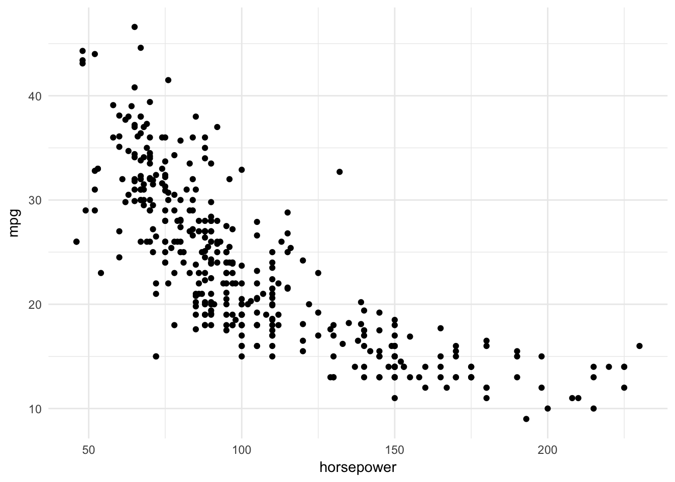
The relationship does not appear to be strictly linear:
ggplot(Auto, aes(horsepower, mpg)) +
geom_point() +
geom_smooth(method = "lm", se = FALSE)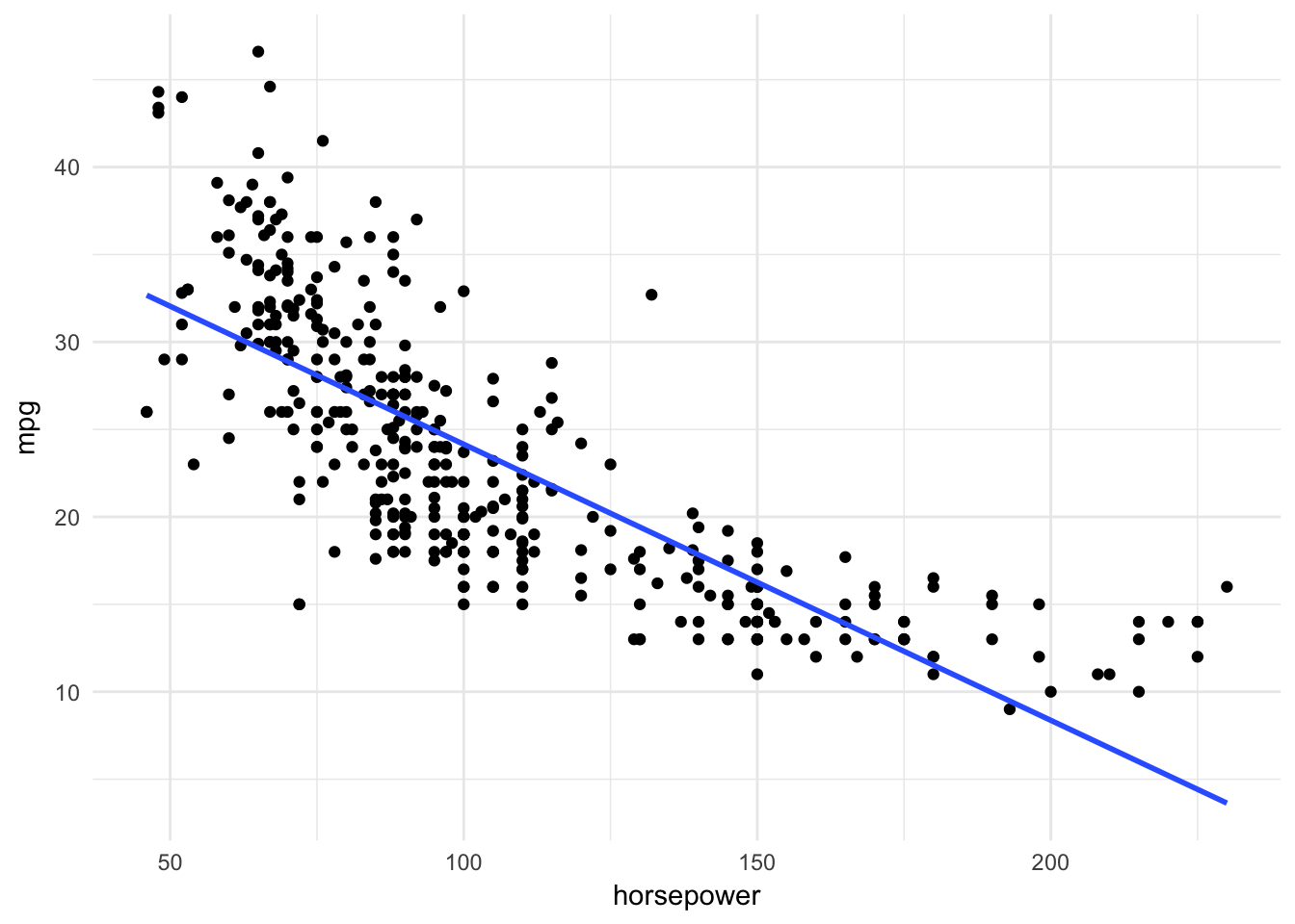
Perhaps by adding quadratic terms to the linear regression we could improve overall model fit. To evaluate the model, we will split the data into a training set and test set, estimate a series of higher-order models, and calculate a test statistic summarizing the accuracy of the estimated mpg. To calculate the accuracy of the model, we will use Mean Squared Error (MSE), defined as
\[MSE = \frac{1}{n} \sum_{i = 1}^{n}{(y_i - \hat{f}(x_i))^2}\]
where:
- \(y_i =\) the observed response value for the \(i\)th observation
- \(\hat{f}(x_i) =\) the predicted response value for the \(i\)th observation given by \(\hat{f}\)
- \(n =\) the total number of observations
Boo math! Actually this is pretty intuitive. All we’re doing is for each observation, calculating the difference between the actual and predicted values for \(y\), squaring that difference, then calculating the average across all observations. An MSE of 0 indicates the model perfectly predicted each observation. The larger the MSE, the more error in the model.
For this task, first we can use modelr::resample_partition() to create training and test sets (using a 50/50 split), then estimate a linear regression model without any quadratic terms.
- I use
set.seed()in the beginning - whenever you are writing a script that involves randomization (here, random subsetting of the data), always set the seed at the beginning of the script. This ensures the results can be reproduced precisely.1 - I also use the
glm()function rather thanlm()- if you don’t change thefamilyparameter, the results oflm()andglm()are exactly the same.2
set.seed(1234)

auto_split <- resample_partition(Auto, c(test = 0.5, train = 0.5))
auto_train <- as_tibble(auto_split$train)
auto_test <- as_tibble(auto_split$test)
auto_lm <- glm(mpg ~ horsepower, data = auto_train)
summary(auto_lm)##
## Call:
## glm(formula = mpg ~ horsepower, data = auto_train)
##
## Deviance Residuals:
## Min 1Q Median 3Q Max
## -12.892 -2.864 -0.545 2.793 13.298
##
## Coefficients:
## Estimate Std. Error t value Pr(>|t|)
## (Intercept) 38.005404 0.921129 41.26 <2e-16 ***
## horsepower -0.140459 0.007968 -17.63 <2e-16 ***
## ---
## Signif. codes: 0 '***' 0.001 '**' 0.01 '*' 0.05 '.' 0.1 ' ' 1
##
## (Dispersion parameter for gaussian family taken to be 20.48452)
##
## Null deviance: 10359.4 on 196 degrees of freedom
## Residual deviance: 3994.5 on 195 degrees of freedom
## AIC: 1157.9
##
## Number of Fisher Scoring iterations: 2To estimate the MSE for a single partition (i.e. for a training or test set), I wrote a special function mse():3
mse <- function(model, data) {
  x <- modelr:::residuals(model, data)
  mean(x ^ 2, na.rm = TRUE)
}mse(auto_lm, auto_test)## [1] 28.57255For a strictly linear model, the MSE for the test set is 28.57. How does this compare to a quadratic model? We can use the poly() function in conjunction with a map() iteration to estimate the MSE for a series of models with higher-order polynomial terms:
# write a custom model function
auto_poly_glm <- function(x){
  glm(mpg ~ poly(horsepower, x), data = auto_train)
}

# estimate models with higher order polynomials
auto_poly_results <- data_frame(terms = 1:5,
                                model = map(terms, auto_poly_glm),
                                MSE = map_dbl(model,
                                              mse,
                                              data = auto_test)
)

# visualize each model
data_grid(Auto, horsepower) %>%
  gather_predictions(`1` = auto_poly_results$model[[1]],
                     `2` = auto_poly_results$model[[2]],
                     `3` = auto_poly_results$model[[3]],
                     `4` = auto_poly_results$model[[4]],
                     `5` = auto_poly_results$model[[5]]) %>%
  ggplot(aes(horsepower, pred)) +
  geom_point(data = Auto, aes(y = mpg), alpha = .1) +
  geom_line(aes(color = model)) +
  scale_color_brewer(type = "qual", palette = "Dark2") +
  labs(x = "Horsepower",
       y = "MPG",
       color = "Highest-order\npolynomial")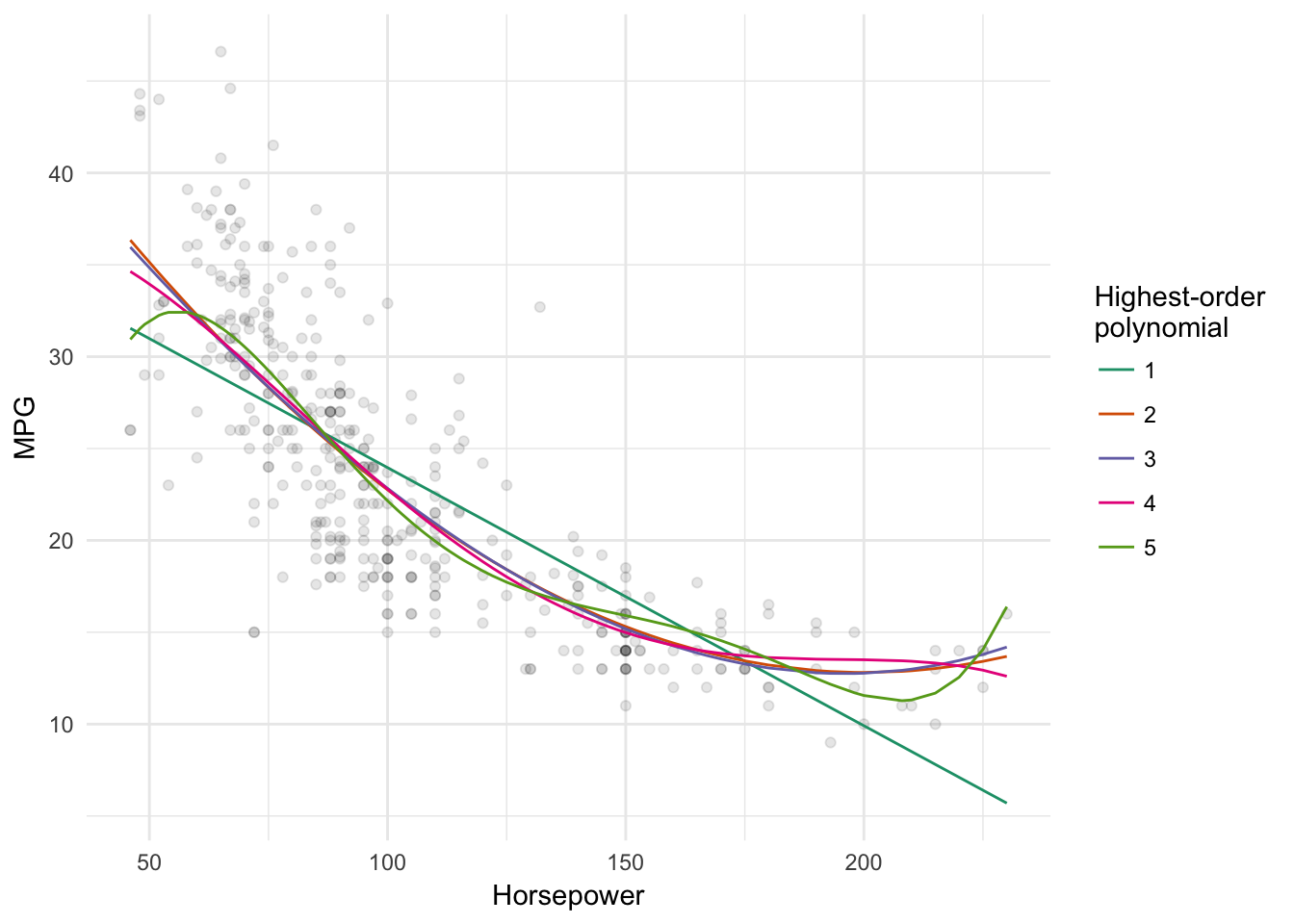
# compare mse
ggplot(auto_poly_results, aes(terms, MSE)) +
  geom_line() +
  labs(title = "Comparing quadratic linear models",
       subtitle = "Using validation set",
       x = "Highest-order polynomial",
       y = "Mean Squared Error")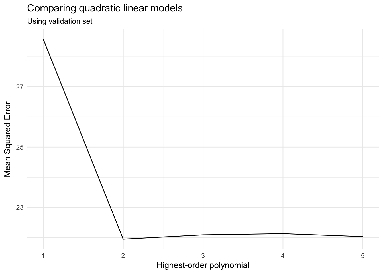
Based on the MSE for the validation (test) set, a polynomial model with a quadratic term (\(\text{horsepower}^2\)) produces the lowest average error. Adding cubic or higher-order terms is just not necessary.
Classification
Recall our efforts to predict passenger survival during the sinking of the Titanic.
library(titanic)
titanic <- as_tibble(titanic_train)

titanic %>%
  head() %>%
knitr::kable()| PassengerId | Survived | Pclass | Name | Sex | Age | SibSp | Parch | Ticket | Fare | Cabin | Embarked |
|---|---|---|---|---|---|---|---|---|---|---|---|
| 1 | 0 | 3 | Braund, Mr. Owen Harris | male | 22 | 1 | 0 | A/5 21171 | 7.2500 | S | |
| 2 | 1 | 1 | Cumings, Mrs. John Bradley (Florence Briggs Thayer) | female | 38 | 1 | 0 | PC 17599 | 71.2833 | C85 | C |
| 3 | 1 | 3 | Heikkinen, Miss. Laina | female | 26 | 0 | 0 | STON/O2. 3101282 | 7.9250 | S | |
| 4 | 1 | 1 | Futrelle, Mrs. Jacques Heath (Lily May Peel) | female | 35 | 1 | 0 | 113803 | 53.1000 | C123 | S |
| 5 | 0 | 3 | Allen, Mr. William Henry | male | 35 | 0 | 0 | 373450 | 8.0500 | S | |
| 6 | 0 | 3 | Moran, Mr. James | male | NA | 0 | 0 | 330877 | 8.4583 | Q |
survive_age_woman_x <- glm(Survived ~ Age * Sex, data = titanic,
                           family = binomial)
summary(survive_age_woman_x)
##
## Call:
## glm(formula = Survived ~ Age * Sex, family = binomial, data = titanic)
##
## Deviance Residuals:
## Min 1Q Median 3Q Max
## -1.9401 -0.7136 -0.5883 0.7626 2.2455
##
## Coefficients:
## Estimate Std. Error z value Pr(>|z|)
## (Intercept) 0.59380 0.31032 1.913 0.05569 .
## Age 0.01970 0.01057 1.863 0.06240 .
## Sexmale -1.31775 0.40842 -3.226 0.00125 **
## Age:Sexmale -0.04112 0.01355 -3.034 0.00241 **
## ---
## Signif. codes: 0 '***' 0.001 '**' 0.01 '*' 0.05 '.' 0.1 ' ' 1
##
## (Dispersion parameter for binomial family taken to be 1)
##
## Null deviance: 964.52 on 713 degrees of freedom
## Residual deviance: 740.40 on 710 degrees of freedom
## (177 observations deleted due to missingness)
## AIC: 748.4
##
## Number of Fisher Scoring iterations: 4We can use the same validation set approach to evaluate the model’s accuracy. For classification models, instead of using MSE we examine the test error rate. That is, of all the predictions generated for the test set, what percentage of predictions are incorrect? The goal is to minimize this value as much as possible (ideally, until we make no errors and our error rate is \(0%\)).
# function to convert log-odds to probabilities
logit2prob <- function(x){
  exp(x) / (1 + exp(x))
}
titanic_split <- resample_partition(titanic, c(test = 0.3, train = 0.7))
map(titanic_split, dim)## $test
## [1] 267 12
##
## $train
## [1] 624 12train_model <- glm(Survived ~ Age * Sex, data = titanic_split$train,
family = binomial)
summary(train_model)##
## Call:
## glm(formula = Survived ~ Age * Sex, family = binomial, data = titanic_split$train)
##
## Deviance Residuals:
## Min 1Q Median 3Q Max
## -2.0027 -0.7056 -0.6274 0.6999 2.0394
##
## Coefficients:
## Estimate Std. Error z value Pr(>|z|)
## (Intercept) 0.86045 0.38879 2.213 0.026886 *
## Age 0.01755 0.01307 1.343 0.179157
## Sexmale -1.83123 0.50484 -3.627 0.000286 ***
## Age:Sexmale -0.02974 0.01642 -1.812 0.070040 .
## ---
## Signif. codes: 0 '***' 0.001 '**' 0.01 '*' 0.05 '.' 0.1 ' ' 1
##
## (Dispersion parameter for binomial family taken to be 1)
##
## Null deviance: 687.03 on 504 degrees of freedom
## Residual deviance: 512.91 on 501 degrees of freedom
## (119 observations deleted due to missingness)
## AIC: 520.91
##
## Number of Fisher Scoring iterations: 4x_test_accuracy <- titanic_split$test %>%
as_tibble() %>%
add_predictions(train_model) %>%
mutate(pred = logit2prob(pred),
pred = as.numeric(pred > .5))
mean(x_test_accuracy$Survived != x_test_accuracy$pred, na.rm = TRUE)## [1] 0.2488038This interactive model generates an error rate of 24.9%. We could compare this error rate to alternative classification models, either other logistic regression models (using different formulas) or a tree-based method.
Drawbacks to validation sets
There are two main problems with validation sets:
Validation estimates of the test error rates can be highly variable depending on which observations are sampled into the training and test sets. See what happens if we repeat the sampling, estimation, and validation procedure for the
Autodata set:mse_variable <- function(Auto){ auto_split <- resample_partition(Auto, c(test = 0.5, train = 0.5)) auto_train <- as_tibble(auto_split$train) auto_test <- as_tibble(auto_split$test) results <- data_frame(terms = 1:5, model = map(terms, auto_poly_glm), MSE = map_dbl(model, mse, data = auto_test)) return(results) } rerun(10, mse_variable(Auto)) %>% bind_rows(.id = "id") %>% ggplot(aes(terms, MSE, color = id)) + geom_line() + labs(title = "Variability of MSE estimates", subtitle = "Using the validation set approach", x = "Degree of Polynomial", y = "Mean Squared Error") + theme(legend.position = "none")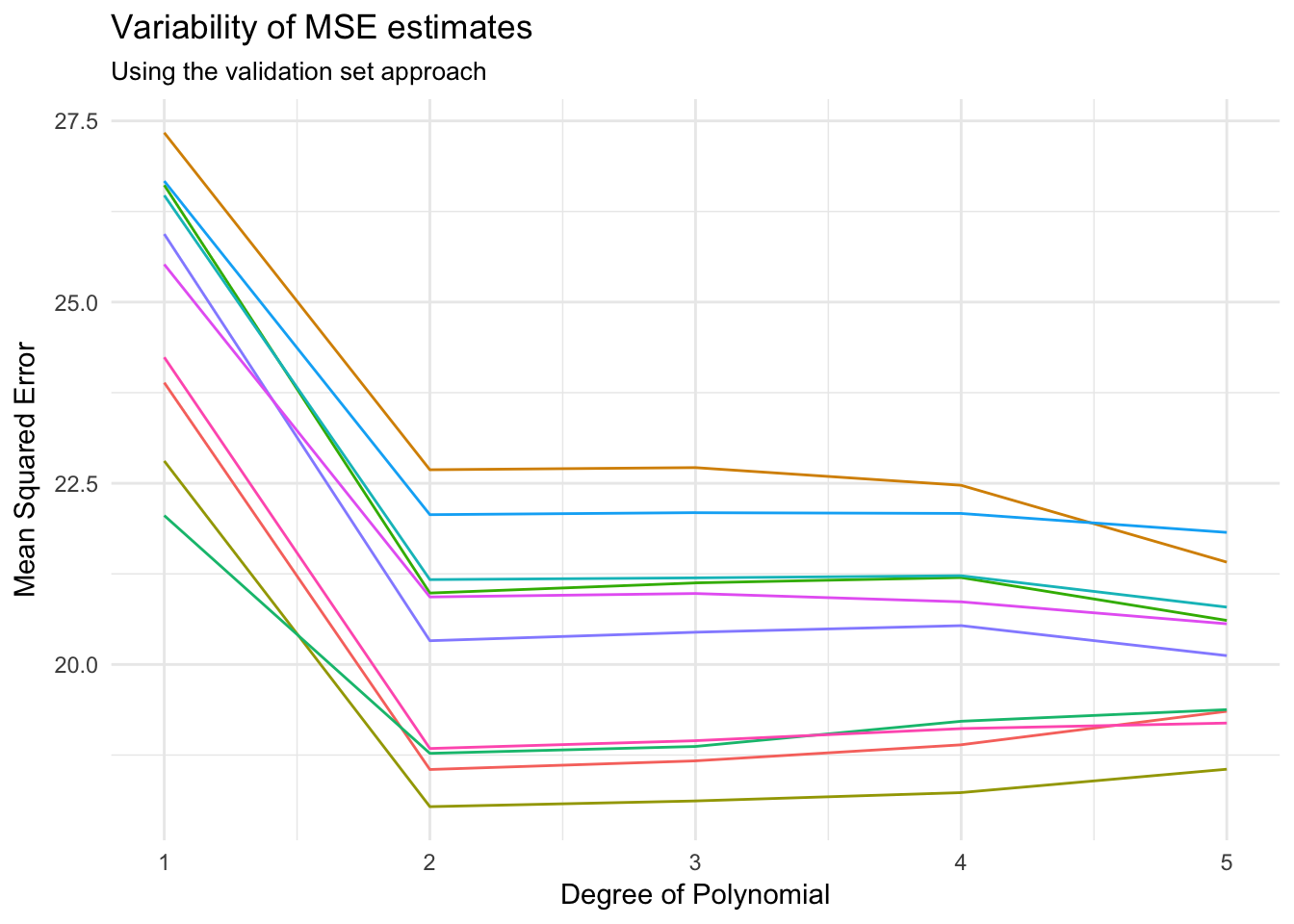
Depending on the specific training/test split, our MSE varies by up to 5.
If you don’t have a large data set, you’ll have to dramatically shrink the size of your training set. Most statistical learning methods perform better with more observations - if you don’t have enough data in the training set, you might overestimate the error rate in the test set.
Leave-one-out cross-validation
An alternative method is leave-one-out cross validation (LOOCV). Like with the validation set approach, you split the data into two parts. However the difference is that you only remove one observation for the test set, and keep all remaining observations in the training set. The statistical learning method is fit on the \(n-1\) training set. You then use the held-out observation to calculate the \(MSE = (y_1 - \hat{y}_1)^2\) which should be an unbiased estimator of the test error. Because this MSE is highly dependent on which observation is held out, we repeat this process for every single observation in the data set. Mathematically, this looks like:
\[CV_{(n)} = \frac{1}{n} \sum_{i = 1}^{n}{MSE_i}\]
This method produces estimates of the error rate that have minimal bias and are relatively steady (i.e. non-varying), unlike the validation set approach where the MSE estimate is highly dependent on the sampling process for training/test sets. LOOCV is also highly flexible and works with any kind of predictive modeling.
Of course the downside is that this method is computationally difficult. You have to estimate \(n\) different models - if you have a large \(n\) or each individual model takes a long time to compute, you may be stuck waiting a long time for the computer to finish its calculations.
LOOCV in linear regression
We can use the crossv_kfold() function in the modelr library to compute the LOOCV of any linear or logistic regression model. It takes two arguments: the data frame and the number of \(k\)-folds (which we will define shortly). For our purposes now, all you need to know is that k should equal the number of observations in the data frame which we can retrieve using the nrow() function. For the Auto dataset, this looks like:
loocv_data <- crossv_kfold(Auto, k = nrow(Auto))Now we estimate the linear model \(k\) times, excluding the holdout test observation, then calculate the MSE:
loocv_models <- map(loocv_data$train, ~ lm(mpg ~ horsepower, data = .))
loocv_mse <- map2_dbl(loocv_models, loocv_data$test, mse)
mean(loocv_mse)
## [1] 24.23151The results of the mapped mse() function is the MSE for each iteration through the data, so there is one MSE for each observation. Calculating the mean() of that vector gives us the LOOCV MSE.
We can also use this method to compare the optimal number of polynomial terms as before.
cv_error <- vector("numeric", 5)
terms <- 1:5

for(i in terms){
  loocv_models <- map(loocv_data$train, ~ lm(mpg ~ poly(horsepower, i),
                                             data = .)
  )
  loocv_mse <- map2_dbl(loocv_models, loocv_data$test, mse)
  cv_error[[i]] <- mean(loocv_mse)
}

cv_mse <- data_frame(terms = terms,
                     cv_MSE = cv_error)
cv_mse
## # A tibble: 5 x 2
## terms cv_MSE
## <int> <dbl>
## 1 1 24.23151
## 2 2 19.24821
## 3 3 19.33498
## 4 4 19.42443
## 5 5 19.03321ggplot(cv_mse, aes(terms, cv_MSE)) +
geom_line() +
labs(title = "Comparing quadratic linear models",
subtitle = "Using LOOCV",
x = "Highest-order polynomial",
y = "Mean Squared Error")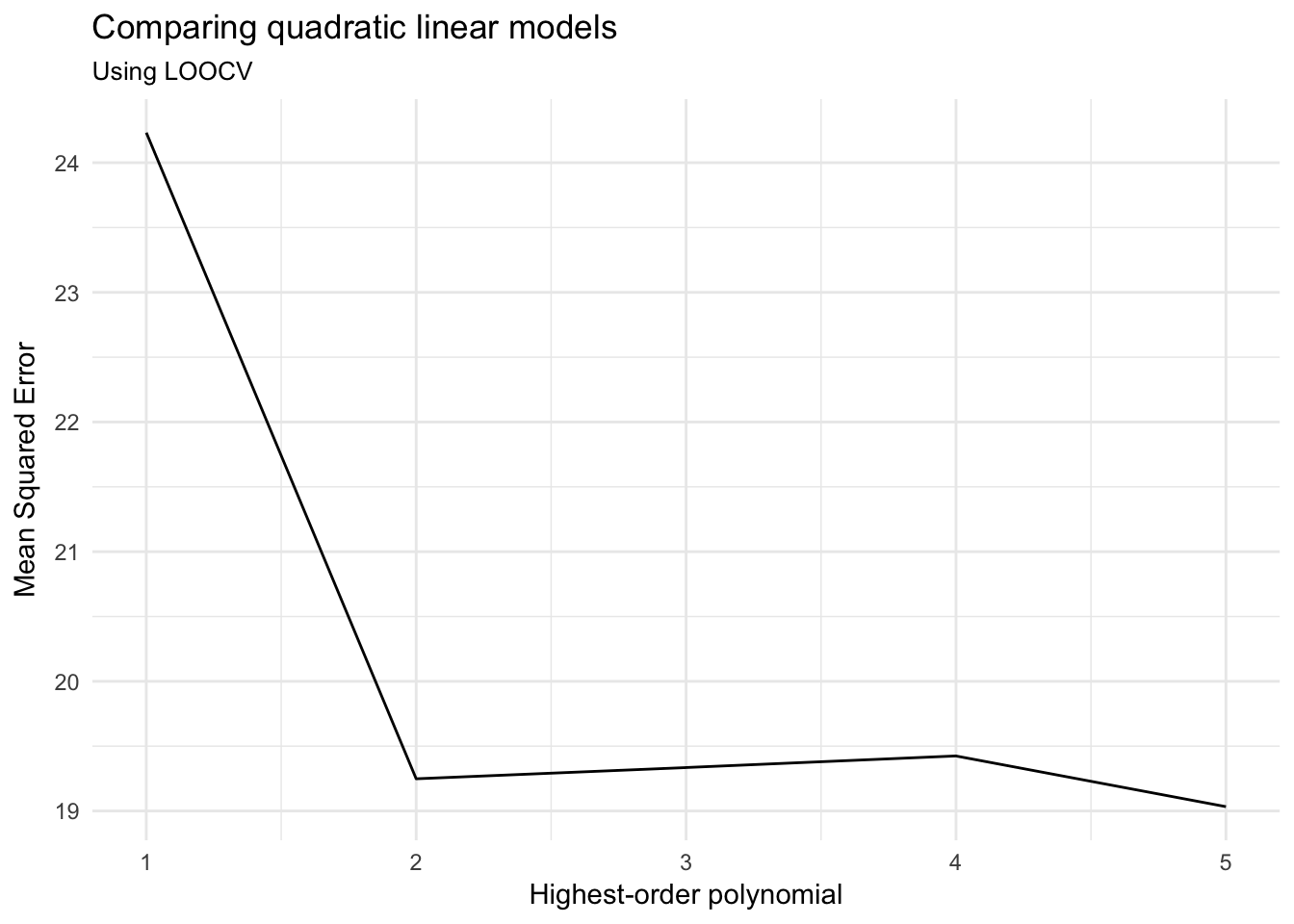
And arrive at a similar conclusion. There may be a very marginal advantage to adding a fifth-order polynomial, but not substantial enough for the additional complexity over a mere second-order polynomial.
LOOCV in classification
Let’s use classification to validate the interactive terms model from before. For technical reasons, we need to use a custom mse.glm() function to properly calculate the MSE for binary response variables:4
mse.glm <- function (model, data){
  residuals.glm <- function(model, data) {
    modelr:::response(model, data) - stats::predict(model,
                                                    data,
                                                    type = "response")
  }

  x <- residuals(model, data)
  mean(x^2, na.rm = TRUE)
}
titanic_loocv <- crossv_kfold(titanic, k = nrow(titanic))
titanic_models <- map(titanic_loocv$train, ~ glm(Survived ~ Age * Sex,
data = .,
family = binomial))
titanic_mse <- map2_dbl(titanic_models, titanic_loocv$test, mse.glm)
mean(titanic_mse, na.rm = TRUE)## [1] 0.1703518In a classification problem, the LOOCV tells us the average error rate based on our predictions. So here, it tells us that the interactive Age * Sex model has a 17% error rate. This is similar to the validation set result (\(24.9\%\))
Exercise: LOOCV in linear regression
Estimate the LOOCV MSE of a linear regression of the relationship between admission rate and cost in the
scorecarddataset.Click for the solution
library(rcfss)

scorecard_loocv <- crossv_kfold(scorecard, k = nrow(scorecard)) %>%
  mutate(model = map(train, ~ lm(cost ~ admrate, data = .)),
         mse = map2_dbl(model, test, mse))
mean(scorecard_loocv$mse, na.rm = TRUE)
## [1] 147752431Estimate the LOOCV MSE of a logistic regression model of voter turnout using only
mhealthas the predictor. Compare this to the LOOCV MSE of a logistic regression model using all available predictors. Which is the better model?Click for the solution
# basic model
mh_loocv_lite <- crossv_kfold(mental_health, k = nrow(mental_health)) %>%
  mutate(model = map(train, ~ glm(vote96 ~ mhealth, data = .,
                                  family = binomial)),
         mse = map2_dbl(model, test, mse.glm))
mean(mh_loocv_lite$mse, na.rm = TRUE)
## [1] 0.2092831# full model mh_loocv_full <- crossv_kfold(mental_health, k = nrow(mental_health)) %>% mutate(model = map(train, ~ glm(vote96 ~ ., data = ., family = binomial)), mse = map2_dbl(model, test, mse.glm)) mean(mh_loocv_full$mse, na.rm = TRUE)## [1] 0.1824597The full model is better and has a lower error rate.
k-fold cross-validation
A less computationally-intensive approach to cross validation is \(k\)-fold cross-validation. Rather than dividing the data into \(n\) groups, one divides the observations into \(k\) groups, or folds, of approximately equal size. The first fold is treated as the validation set, and the model is estimated on the remaining \(k-1\) folds. This process is repeated \(k\) times, with each fold serving as the validation set precisely once. The \(k\)-fold CV estimate is calculated by averaging the MSE values for each fold:
\[CV_{(k)} = \frac{1}{k} \sum_{i = 1}^{k}{MSE_i}\]
As you probably figured out by now, LOOCV is the special case of \(k\)-fold cross-validation where \(k = n\). More typically researchers will use \(k=5\) or \(k=10\) depending on the size of the data set and the complexity of the statistical model.
k-fold CV in linear regression
Let’s go back to the Auto data set. Instead of LOOCV, let’s use 10-fold CV to compare the different polynomial models.
cv10_data <- crossv_kfold(Auto, k = 10)

cv_error_fold10 <- vector("numeric", 5)
terms <- 1:5

for(i in terms){
  cv10_models <- map(cv10_data$train, ~ lm(mpg ~ poly(horsepower, i),
                                           data = .)
  )
  cv10_mse <- map2_dbl(cv10_models, cv10_data$test, mse)
  cv_error_fold10[[i]] <- mean(cv10_mse)
}

cv_error_fold10
## [1] 24.46588 19.37772 19.51389 19.82524 19.36807How do these results compare to the LOOCV values?
data_frame(terms = terms,
           loocv = cv_error,
           fold10 = cv_error_fold10) %>%
  gather(method, MSE, loocv:fold10) %>%
  ggplot(aes(terms, MSE, color = method)) +
  geom_line() +
  labs(title = "MSE estimates",
       x = "Degree of Polynomial",
       y = "Mean Squared Error",
       color = "CV Method")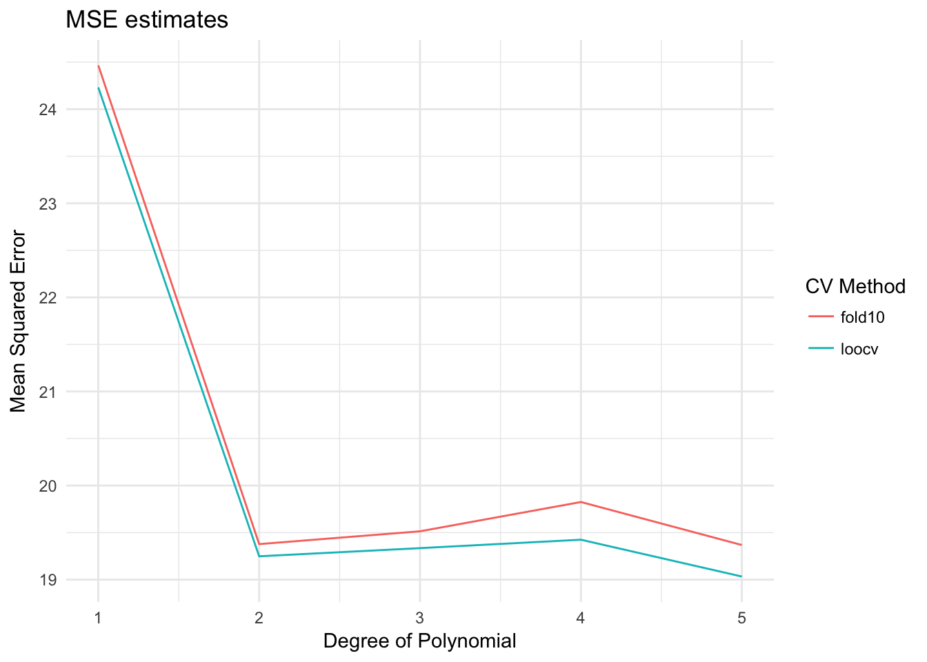
Pretty much the same results.
Computational speed of LOOCV vs. \(k\)-fold CV
LOOCV
library(profvis)

profvis({
  cv_error <- vector("numeric", 5)
  terms <- 1:5

  for(i in terms){
    loocv_models <- map(loocv_data$train, ~ lm(mpg ~ poly(horsepower, i), data = .))
    loocv_mse <- map2_dbl(loocv_models, loocv_data$test, mse)
    cv_error[[i]] <- mean(loocv_mse)
  }
})
10-fold CV
profvis({
  cv_error_fold10 <- vector("numeric", 5)
  terms <- 1:5

  for(i in terms){
    cv10_models <- map(cv10_data$train, ~ lm(mpg ~ poly(horsepower, i), data = .))
    cv10_mse <- map2_dbl(cv10_models, cv10_data$test, mse)
    cv_error_fold10[[i]] <- mean(cv10_mse)
  }
})
On my machine, 10-fold CV was about 40 times faster than LOOCV. Again, estimating \(k=10\) models is going to be much easier than estimating \(k=392\) models.
k-fold CV in logistic regression
You’ve gotten the idea by now, but let’s do it one more time on our interactive Titanic model.
titanic_kfold <- crossv_kfold(titanic, k = 10)
titanic_models <- map(titanic_kfold$train, ~ glm(Survived ~ Age * Sex,
                                                 data = .,
                                                 family = binomial))
titanic_mse <- map2_dbl(titanic_models, titanic_kfold$test, mse.glm)
mean(titanic_mse, na.rm = TRUE)
## [1] 0.1693387Not a large difference from the LOOCV approach, but it take much less time to compute.
Exercise: k-fold CV
Estimate the 10-fold CV MSE of a linear regression of the relationship between admission rate and cost in the
scorecarddataset.Click for the solution
scorecard_cv10 <- crossv_kfold(scorecard, k = 10) %>%
  mutate(model = map(train, ~ lm(cost ~ admrate, data = .)),
         mse = map2_dbl(model, test, mse))
mean(scorecard_cv10$mse, na.rm = TRUE)
## [1] 147794005Estimate the 10-fold CV MSE of a logistic regression model of voter turnout using only
mhealthas the predictor. Compare this to the LOOCV MSE of a logistic regression model using all available predictors. Which is the better model?Click for the solution
# basic model
mh_cv10_lite <- crossv_kfold(mental_health, k = 10) %>%
  mutate(model = map(train, ~ glm(vote96 ~ mhealth, data = .,
                                  family = binomial)),
         mse = map2_dbl(model, test, mse.glm))
mean(mh_cv10_lite$mse, na.rm = TRUE)
## [1] 0.2093087# full model mh_cv10_full <- crossv_kfold(mental_health, k = 10) %>% mutate(model = map(train, ~ glm(vote96 ~ ., data = ., family = binomial)), mse = map2_dbl(model, test, mse.glm)) mean(mh_cv10_full$mse, na.rm = TRUE)## [1] 0.1819416
Session Info
devtools::session_info()## setting value
## version R version 3.4.3 (2017-11-30)
## system x86_64, darwin15.6.0
## ui X11
## language (EN)
## collate en_US.UTF-8
## tz America/Chicago
## date 2018-04-24
##
## package * version date source
## assertthat 0.2.0 2017-04-11 CRAN (R 3.4.0)
## backports 1.1.2 2017-12-13 CRAN (R 3.4.3)
## base * 3.4.3 2017-12-07 local
## bindr 0.1.1 2018-03-13 CRAN (R 3.4.3)
## bindrcpp 0.2.2.9000 2018-04-08 Github (krlmlr/bindrcpp@bd5ae73)
## broom * 0.4.4 2018-03-29 CRAN (R 3.4.3)
## cellranger 1.1.0 2016-07-27 CRAN (R 3.4.0)
## cli 1.0.0 2017-11-05 CRAN (R 3.4.2)
## colorspace 1.3-2 2016-12-14 CRAN (R 3.4.0)
## compiler 3.4.3 2017-12-07 local
## crayon 1.3.4 2017-10-03 Github (gaborcsardi/crayon@b5221ab)
## datasets * 3.4.3 2017-12-07 local
## devtools 1.13.5 2018-02-18 CRAN (R 3.4.3)
## digest 0.6.15 2018-01-28 CRAN (R 3.4.3)
## dplyr * 0.7.4.9003 2018-04-08 Github (tidyverse/dplyr@b7aaa95)
## evaluate 0.10.1 2017-06-24 CRAN (R 3.4.1)
## forcats * 0.3.0 2018-02-19 CRAN (R 3.4.3)
## foreign 0.8-69 2017-06-22 CRAN (R 3.4.3)
## ggplot2 * 2.2.1.9000 2018-04-24 Github (tidyverse/ggplot2@3c9c504)
## glue 1.2.0 2017-10-29 CRAN (R 3.4.2)
## graphics * 3.4.3 2017-12-07 local
## grDevices * 3.4.3 2017-12-07 local
## grid 3.4.3 2017-12-07 local
## gtable 0.2.0 2016-02-26 CRAN (R 3.4.0)
## haven 1.1.1 2018-01-18 CRAN (R 3.4.3)
## hms 0.4.2 2018-03-10 CRAN (R 3.4.3)
## htmltools 0.3.6 2017-04-28 CRAN (R 3.4.0)
## httr 1.3.1 2017-08-20 CRAN (R 3.4.1)
## jsonlite 1.5 2017-06-01 CRAN (R 3.4.0)
## knitr 1.20 2018-02-20 CRAN (R 3.4.3)
## lattice 0.20-35 2017-03-25 CRAN (R 3.4.3)
## lazyeval 0.2.1 2017-10-29 CRAN (R 3.4.2)
## lubridate 1.7.4 2018-04-11 CRAN (R 3.4.3)
## magrittr 1.5 2014-11-22 CRAN (R 3.4.0)
## memoise 1.1.0 2017-04-21 CRAN (R 3.4.0)
## methods * 3.4.3 2017-12-07 local
## mnormt 1.5-5 2016-10-15 CRAN (R 3.4.0)
## modelr * 0.1.1 2017-08-10 local
## munsell 0.4.3 2016-02-13 CRAN (R 3.4.0)
## nlme 3.1-137 2018-04-07 CRAN (R 3.4.4)
## parallel 3.4.3 2017-12-07 local
## pillar 1.2.1 2018-02-27 CRAN (R 3.4.3)
## pkgconfig 2.0.1 2017-03-21 CRAN (R 3.4.0)
## plyr 1.8.4 2016-06-08 CRAN (R 3.4.0)
## psych 1.8.3.3 2018-03-30 CRAN (R 3.4.4)
## purrr * 0.2.4 2017-10-18 CRAN (R 3.4.2)
## R6 2.2.2 2017-06-17 CRAN (R 3.4.0)
## Rcpp 0.12.16 2018-03-13 CRAN (R 3.4.4)
## readr * 1.1.1 2017-05-16 CRAN (R 3.4.0)
## readxl 1.0.0 2017-04-18 CRAN (R 3.4.0)
## reshape2 1.4.3 2017-12-11 CRAN (R 3.4.3)
## rlang 0.2.0.9001 2018-04-24 Github (r-lib/rlang@82b2727)
## rmarkdown 1.9 2018-03-01 CRAN (R 3.4.3)
## rprojroot 1.3-2 2018-01-03 CRAN (R 3.4.3)
## rstudioapi 0.7 2017-09-07 CRAN (R 3.4.1)
## rvest 0.3.2 2016-06-17 CRAN (R 3.4.0)
## scales 0.5.0.9000 2018-04-24 Github (hadley/scales@d767915)
## stats * 3.4.3 2017-12-07 local
## stringi 1.1.7 2018-03-12 CRAN (R 3.4.3)
## stringr * 1.3.0 2018-02-19 CRAN (R 3.4.3)
## tibble * 1.4.2 2018-01-22 CRAN (R 3.4.3)
## tidyr * 0.8.0 2018-01-29 CRAN (R 3.4.3)
## tidyselect 0.2.4 2018-02-26 CRAN (R 3.4.3)
## tidyverse * 1.2.1 2017-11-14 CRAN (R 3.4.2)
## tools 3.4.3 2017-12-07 local
## utils * 3.4.3 2017-12-07 local
## withr 2.1.2 2018-04-24 Github (jimhester/withr@79d7b0d)
## xml2 1.2.0 2018-01-24 CRAN (R 3.4.3)
## yaml 2.1.18 2018-03-08 CRAN (R 3.4.4)The actual value you use is irrelevant. Just be sure to set it in the script, otherwise R will randomly pick one each time you start a new session.↩
The default
familyforglm()isgaussian(), or the Gaussian distribution. You probably know it by its other name, the Normal distribution.↩This function can also be loaded via the
rcfsslibrary. Be sure to update your package to the latest version to make sure the function is available.↩
This work is licensed under the CC BY-NC 4.0 Creative Commons License.