Text analysis: supervised classification
library(tidyverse)
library(tidytext)
library(stringr)
library(caret)
library(tm)

set.seed(1234)
theme_set(theme_minimal())
A common task in social science involves hand-labeling sets of documents for specific variables (e.g. manual coding). In previous years, this required hiring a set of research assistants and training them to read and evaluate text by hand. It was expensive, prone to error, required extensive data quality checks, and was infeasible if you had an extremely large corpus of text that required classification.
Alternatively, we can now use statistical learning models to classify text into specific sets of categories. This is known as supervised learning. The basic process is:
- Hand-code a small set of documents (say \(1000\)) for whatever variable(s) you care about
- Train a statistical learning model on the hand-coded data, using the variable as the outcome of interest and the text features of the documents as the predictors
- Evaluate the effectiveness of the statistical learning model via a resampling method
- Once you have trained a model with sufficient predictive accuracy, apply the model to the remaining set of documents that have never been hand-coded (say \(1000000\))
Sample set of documents: USCongress
# get USCongress data
data(USCongress, package = "RTextTools")

(congress <- as_tibble(USCongress) %>%
    mutate(text = as.character(text)))
## # A tibble: 4,449 x 6
## ID cong billnum h_or_sen major
## <int> <int> <int> <fctr> <int>
## 1 1 107 4499 HR 18
## 2 2 107 4500 HR 18
## 3 3 107 4501 HR 18
## 4 4 107 4502 HR 18
## 5 5 107 4503 HR 5
## 6 6 107 4504 HR 21
## 7 7 107 4505 HR 15
## 8 8 107 4506 HR 18
## 9 9 107 4507 HR 18
## 10 10 107 4508 HR 18
## # ... with 4,439 more rows, and 1 more variables: text <chr>USCongress from the RTextTools package contains a sample of hand-labeled bills from the United States Congress. For each bill we have a text description of the bill’s purpose (e.g. “To amend the Immigration and Nationality Act in regard to Caribbean-born immigrants.”) as well as the bill’s major policy topic code corresponding to the subject of the bill. There are 20 major policy topics according to this coding scheme (e.g. Macroeconomics, Civil Rights, Health). These topic codes have been labeled by hand. The current dataset only contains a sample of bills from the 107th Congress (2001-03). If we wanted to obtain policy topic codes for all bills introduced over a longer period, we would have to manually code tens of thousands if not millions of bill descriptions. Clearly a task outside of our capabilities.
Instead, we can build a statistical learning model which predicts the major topic code of a bill given its text description. These notes outline a potential tidytext workflow for such an approach.
Create tidy text data frame
First we convert USCongress into a tidy text data frame.
(congress_tokens <- congress %>%
   unnest_tokens(output = word, input = text) %>%
   # remove numbers
   filter(!str_detect(word, "^[0-9]*$")) %>%
   # remove stop words
   anti_join(stop_words) %>%
   # stem the words
   mutate(word = SnowballC::wordStem(word)))
## Joining, by = "word"## # A tibble: 58,820 x 6
## ID cong billnum h_or_sen major word
## <int> <int> <int> <fctr> <int> <chr>
## 1 1 107 4499 HR 18 suspend
## 2 1 107 4499 HR 18 temporarili
## 3 1 107 4499 HR 18 duti
## 4 1 107 4499 HR 18 fast
## 5 1 107 4499 HR 18 magenta
## 6 1 107 4499 HR 18 stage
## 7 2 107 4500 HR 18 suspend
## 8 2 107 4500 HR 18 temporarili
## 9 2 107 4500 HR 18 duti
## 10 2 107 4500 HR 18 fast
## # ... with 58,810 more rowsNotice there are a few key steps involved here:
unnest_tokens(output = word, input = text)- converts the data frame to a tidy text data frame and automatically converts all tokens to lowercasefilter(!str_detect(word, "^[0-9]*$"))- removes all tokens which are strictly numbers. Numbers are generally not useful features in classifying documents (though sometimes they may be useful - you can compare results with and without numbers)anti_join(stop_words)- remove common stop words that are uninformative and will likely not be useful in predicting major topic codesmutate(word = SnowballC::wordStem(word)))- uses the Porter stemming algorithm to stem all the tokens to their root word
Most of these steps are to reduce the number of text features in the set of documents. This is necessary because as you increase the number of observations (i.e. documents) and variables/features (i.e. tokens/words), the resulting statistical learning model will become more complex and harder to compute. Given a large enough corpus or set of variables, you may not be able to estimate many statistical learning models with your local computer - you would need to offload the work to a remote computing cluster.
Create document-term matrix
tidy text data frames are one-row-per-token, but for statistical learning algorithms we need our data in a one-row-per-document format. That is, a document-term matrix. We can use cast_dtm() to create a document-term matrix.
(congress_dtm <- congress_tokens %>%
   # get count of each token in each document
   count(ID, word) %>%
   # create a document-term matrix with all features and tf weighting
   cast_dtm(document = ID, term = word, value = n))
## <<DocumentTermMatrix (documents: 4449, terms: 4902)>>
## Non-/sparse entries: 55033/21753965
## Sparsity : 100%
## Maximal term length: 24
## Weighting : term frequency (tf)Weighting
The default approach is to use term frequency (tf) weighting, or a simple count of how frequently a word occurs in a document. An alternative approach is term frequency inverse document frequency (tf-idf), which is the frequency of a term adjusted for how rarely it is used. To generate tf-idf and use this for the document-term matrix, we can change the weighting function in cast_dtm():1
congress_tokens %>%
  # get count of each token in each document
  count(ID, word) %>%
  # create a document-term matrix with all features and tf-idf weighting
  cast_dtm(document = ID, term = word, value = n,
           weighting = tm::weightTfIdf)
## <<DocumentTermMatrix (documents: 4449, terms: 4902)>>
## Non-/sparse entries: 55033/21753965
## Sparsity : 100%
## Maximal term length: 24
## Weighting : term frequency - inverse document frequency (normalized) (tf-idf)For now, let’s just continue to use the term frequency approach. But it is a good idea to compare the results of tf vs. tf-idf to see if one method improves model performance over the other method.
Sparsity
Another approach to reducing model complexity is to remove sparse terms from the model. That is, remove tokens which do not appear across many documents. It is similar to using tf-idf weighting, but directly deletes sparse variables from the document-term matrix. This results in a statistical learning model with a much smaller set of variables.
The tm package contains the removeSparseTerms() function, which does this task. The first argument is a document-term matrix, and the second argument defines the maximal allowed sparsity in the range from 0 to 1. So for instance, sparse = .99 would remove any tokens which are missing from more than \(99%\) of the documents in the corpus. Notice the effect changing this value has on the number of variables (tokens) retained in the document-term matrix:
removeSparseTerms(congress_dtm, sparse = .99)## <<DocumentTermMatrix (documents: 4449, terms: 209)>>
## Non-/sparse entries: 33794/896047
## Sparsity : 96%
## Maximal term length: 11
## Weighting : term frequency (tf)removeSparseTerms(congress_dtm, sparse = .95)## <<DocumentTermMatrix (documents: 4449, terms: 28)>>
## Non-/sparse entries: 18447/106125
## Sparsity : 85%
## Maximal term length: 11
## Weighting : term frequency (tf)removeSparseTerms(congress_dtm, sparse = .90)## <<DocumentTermMatrix (documents: 4449, terms: 16)>>
## Non-/sparse entries: 14917/56267
## Sparsity : 79%
## Maximal term length: 9
## Weighting : term frequency (tf)It will be tough to build an effective model with just 16 tokens. Normal values for sparse are generally around \(.99\). Let’s use that to create and store our final document-term matrix.
congress_dtm <- removeSparseTerms(congress_dtm, sparse = .99)Exploratory analysis
Before building a fancy schmancy statistical model, we can first investigate if there are certain terms or tokens associated with each major topic category. We can do this purely with tidytext tools: we directly calculate the tf-idf for each term treating each major topic code as the document, rather than the individual bill. Then we can visualize the tokens with the highest tf-idf associated with each topic.2
To calculate tf-idf directly in the data frame, first we count() the frequency each token appears in bills from each major topic code, then use bind_tf_idf() to calculate the tf-idf for each token in each topic:3
(congress_tfidf <- congress_tokens %>%
   count(major, word) %>%
   bind_tf_idf(term_col = word, document_col = major, n_col = n))
## # A tibble: 13,190 x 6
## major word n tf idf tf_idf
## <int> <chr> <int> <dbl> <dbl> <dbl>
## 1 1 25,000 1 0.000483559 1.8971200 0.0009173694
## 2 1 3,500,000 1 0.000483559 2.9957323 0.0014486133
## 3 1 38.6 1 0.000483559 2.9957323 0.0014486133
## 4 1 abolish 1 0.000483559 2.3025851 0.0011134357
## 5 1 abroad 1 0.000483559 1.8971200 0.0009173694
## 6 1 abus 2 0.000967118 1.0498221 0.0010153019
## 7 1 acceler 1 0.000483559 1.0498221 0.0005076509
## 8 1 account 6 0.002901354 0.2231436 0.0006474184
## 9 1 accur 1 0.000483559 1.0498221 0.0005076509
## 10 1 acquir 2 0.000967118 1.3862944 0.0013407102
## # ... with 13,180 more rowsNow all we need to do is plot the words with the highest tf-idf scores for each category. Since there are 20 major topics and a 20 panel facet graph is very dense, let’s just look at four of the categories:
# sort the data frame and convert word to a factor column
plot_congress <- congress_tfidf %>%
  arrange(desc(tf_idf)) %>%
  mutate(word = factor(word, levels = rev(unique(word))))

# graph the top 10 tokens for 4 categories
plot_congress %>%
  filter(major %in% c(1:3, 6)) %>%
  mutate(major = factor(major, levels = c(1:3, 6),
                        labels = c("Macroeconomics", "Civil Rights",
                                   "Health", "Education"))) %>%
  group_by(major) %>%
  top_n(10) %>%
  ungroup() %>%
  ggplot(aes(word, tf_idf)) +
  geom_col() +
  labs(x = NULL, y = "tf-idf") +
  facet_wrap(~major, scales = "free") +
  coord_flip()
## Selecting by tf_idf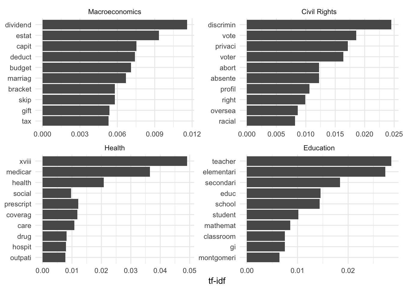
Do these make sense? I think they do (well, some of them). This suggests a statistical learning model may find these tokens useful in predicting major topic codes.
Estimate model
Now to estimate the model, we return to the caret package. Let’s try a random forest model first. Here is the syntax for estimating the model:
congress_rf <- train(x = as.matrix(congress_dtm),
                     y = factor(congress$major),
                     method = "rf",
                     ntree = 200,
                     trControl = trainControl(method = "oob"))
Note the differences from how we specified them before with a standard data frame.
x = as.matrix(congress_dtm)- instead of using a formula, we pass the independent and dependent variables separately intotrain().xneeds to be a simple matrix, data frame, or sparse matrix. These are specific types of objects in R.congress_dtmis aDocumentTermMatrix, so we useas.matrix()to convert it to a simple matrix.y = factor(congress$major)- we return to the originalcongressdata frame to obtain the vector of outcome values for each document. Here, this is the major topic code associated with each bill. The important thing is that the order of documents inxremains the same as the order of documents iny, so that each document is associated with the correct outcome. Becausecongress$majoris a numeric vector, we need to convert it to a factor vector so that we perform classification (and not regression).
Otherwise everything else is the same as before. Notice how long it takes to build a random forest model with 10 trees, compared to a more typical random forest model with 200 trees:
system.time({
  congress_rf_10 <- train(x = as.matrix(congress_dtm),
                          y = factor(congress$major),
                          method = "rf",
                          ntree = 10,
                          trControl = trainControl(method = "oob"))
})
## Loading required package: randomForest## randomForest 4.6-12## Type rfNews() to see new features/changes/bug fixes.##
## Attaching package: 'randomForest'## The following object is masked from 'package:dplyr':
##
## combine## The following object is masked from 'package:ggplot2':
##
## margin## user system elapsed
## 10.832 0.188 11.201system.time({
congress_rf_200 <- train(x = as.matrix(congress_dtm),
y = factor(congress$major),
method = "rf",
ntree = 200,
trControl = trainControl(method = "oob"))
})## user system elapsed
## 188.377 1.873 198.240This is why it is important to remove sparse features and simplify the document-term matrix as much as possible - the more text features and observations in the document-term matrix, the longer it takes to train the model.
Otherwise, the result is no different from a model trained on categorical or continuous variables. We can generate the same diagnostics information:
congress_rf_200$finalModel##
## Call:
## randomForest(x = x, y = y, ntree = 200, mtry = param$mtry)
## Type of random forest: classification
## Number of trees: 200
## No. of variables tried at each split: 105
##
## OOB estimate of error rate: 32.64%
## Confusion matrix:
## 1 2 3 4 5 6 7 8 10 12 13 14 15 16 17 18 19 20 21 99
## 1 106 0 2 0 4 3 2 4 6 9 0 3 10 2 2 3 0 6 1 0
## 2 1 19 5 0 5 4 5 1 2 7 3 2 5 6 4 1 1 9 4 0
## 3 3 1 536 3 10 10 4 1 5 8 6 3 8 10 1 0 0 4 4 0
## 4 2 0 9 92 4 1 4 1 1 2 0 1 1 0 1 5 2 1 6 0
## 5 7 2 12 2 152 12 5 1 9 11 2 1 6 7 6 7 4 7 8 1
## 6 7 1 7 0 8 165 1 0 2 11 1 1 3 2 2 4 2 1 4 0
## 7 3 2 6 5 4 3 105 6 9 7 1 1 7 3 4 2 4 5 24 0
## 8 7 1 1 1 3 1 3 99 2 3 1 2 2 1 1 1 1 2 6 0
## 10 5 1 0 2 4 1 6 2 100 12 0 0 6 3 2 4 3 16 4 0
## 12 10 2 17 5 10 8 8 0 6 149 3 3 13 3 4 8 6 28 5 3
## 13 4 0 5 0 6 0 3 2 1 2 62 2 1 0 1 1 1 2 1 0
## 14 1 0 1 2 5 2 2 1 4 1 1 45 4 2 3 2 0 2 2 0
## 15 14 7 8 6 15 2 7 4 6 16 1 2 149 3 7 11 6 11 3 1
## 16 1 5 2 0 6 4 4 2 5 6 2 1 5 137 0 8 6 18 7 0
## 17 4 0 2 1 6 3 4 1 3 10 1 1 3 1 42 1 1 2 3 1
## 18 0 0 1 2 1 2 5 3 2 1 0 0 2 2 0 371 7 2 1 0
## 19 2 0 3 2 10 5 4 0 4 8 0 0 2 5 0 9 52 4 11 0
## 20 10 1 7 1 15 4 5 2 7 27 1 3 12 13 4 11 1 236 19 1
## 21 7 2 5 2 4 4 24 1 8 7 1 4 4 13 3 9 4 15 355 0
## 99 0 0 0 0 1 0 0 0 1 0 0 0 0 1 1 0 0 0 1 25
## class.error
## 1 0.34969325
## 2 0.77380952
## 3 0.13128039
## 4 0.30827068
## 5 0.41984733
## 6 0.25675676
## 7 0.47761194
## 8 0.28260870
## 10 0.41520468
## 12 0.48797251
## 13 0.34042553
## 14 0.43750000
## 15 0.46594982
## 16 0.37442922
## 17 0.53333333
## 18 0.07711443
## 19 0.57024793
## 20 0.37894737
## 21 0.24788136
## 99 0.16666667varImpPlot(congress_rf_200$finalModel)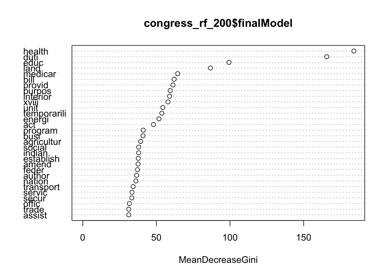
And if we had a test set of observations (or a set of congressional bills never previously hand-coded), we could use this model to predict their major topic codes.
Session Info
devtools::session_info()## Session info -------------------------------------------------------------## setting value
## version R version 3.4.1 (2017-06-30)
## system x86_64, darwin15.6.0
## ui X11
## language (EN)
## collate en_US.UTF-8
## tz America/Chicago
## date 2017-11-21## Packages -----------------------------------------------------------------## package * version date source
## assertthat 0.2.0 2017-04-11 CRAN (R 3.4.0)
## backports 1.1.0 2017-05-22 CRAN (R 3.4.0)
## base * 3.4.1 2017-07-07 local
## bindr 0.1 2016-11-13 CRAN (R 3.4.0)
## bindrcpp * 0.2 2017-06-17 CRAN (R 3.4.0)
## boxes 0.0.0.9000 2017-07-19 Github (r-pkgs/boxes@03098dc)
## broom 0.4.2 2017-08-09 local
## car 2.1-5 2017-07-04 CRAN (R 3.4.1)
## caret * 6.0-76 2017-04-18 CRAN (R 3.4.0)
## cellranger 1.1.0 2016-07-27 CRAN (R 3.4.0)
## clisymbols 1.2.0 2017-05-21 cran (@1.2.0)
## codetools 0.2-15 2016-10-05 CRAN (R 3.4.1)
## colorspace 1.3-2 2016-12-14 CRAN (R 3.4.0)
## compiler 3.4.1 2017-07-07 local
## crayon 1.3.4 2017-10-03 Github (gaborcsardi/crayon@b5221ab)
## datasets * 3.4.1 2017-07-07 local
## devtools 1.13.3 2017-08-02 CRAN (R 3.4.1)
## digest 0.6.12 2017-01-27 CRAN (R 3.4.0)
## dplyr * 0.7.4.9000 2017-10-03 Github (tidyverse/dplyr@1a0730a)
## evaluate 0.10.1 2017-06-24 CRAN (R 3.4.1)
## forcats * 0.2.0 2017-01-23 CRAN (R 3.4.0)
## foreach 1.4.3 2015-10-13 CRAN (R 3.4.0)
## foreign 0.8-69 2017-06-22 CRAN (R 3.4.1)
## ggplot2 * 2.2.1 2016-12-30 CRAN (R 3.4.0)
## glue 1.1.1 2017-06-21 CRAN (R 3.4.1)
## graphics * 3.4.1 2017-07-07 local
## grDevices * 3.4.1 2017-07-07 local
## grid 3.4.1 2017-07-07 local
## gtable 0.2.0 2016-02-26 CRAN (R 3.4.0)
## haven 1.1.0 2017-07-09 CRAN (R 3.4.1)
## hms 0.3 2016-11-22 CRAN (R 3.4.0)
## htmltools 0.3.6 2017-04-28 CRAN (R 3.4.0)
## httr 1.3.1 2017-08-20 CRAN (R 3.4.1)
## iterators 1.0.8 2015-10-13 CRAN (R 3.4.0)
## janeaustenr 0.1.5 2017-06-10 CRAN (R 3.4.0)
## jsonlite 1.5 2017-06-01 CRAN (R 3.4.0)
## knitr 1.17 2017-08-10 cran (@1.17)
## lattice * 0.20-35 2017-03-25 CRAN (R 3.4.1)
## lazyeval 0.2.0 2016-06-12 CRAN (R 3.4.0)
## lme4 1.1-13 2017-04-19 CRAN (R 3.4.0)
## lubridate 1.6.0 2016-09-13 CRAN (R 3.4.0)
## magrittr 1.5 2014-11-22 CRAN (R 3.4.0)
## MASS 7.3-47 2017-02-26 CRAN (R 3.4.1)
## Matrix 1.2-11 2017-08-16 CRAN (R 3.4.1)
## MatrixModels 0.4-1 2015-08-22 CRAN (R 3.4.0)
## memoise 1.1.0 2017-04-21 CRAN (R 3.4.0)
## methods * 3.4.1 2017-07-07 local
## mgcv 1.8-18 2017-07-28 CRAN (R 3.4.1)
## minqa 1.2.4 2014-10-09 CRAN (R 3.4.0)
## mnormt 1.5-5 2016-10-15 CRAN (R 3.4.0)
## ModelMetrics 1.1.0 2016-08-26 CRAN (R 3.4.0)
## modelr 0.1.1 2017-08-10 local
## munsell 0.4.3 2016-02-13 CRAN (R 3.4.0)
## nlme 3.1-131 2017-02-06 CRAN (R 3.4.1)
## nloptr 1.0.4 2014-08-04 CRAN (R 3.4.0)
## NLP * 0.1-11 2017-08-15 CRAN (R 3.4.1)
## nnet 7.3-12 2016-02-02 CRAN (R 3.4.1)
## parallel 3.4.1 2017-07-07 local
## pbkrtest 0.4-7 2017-03-15 CRAN (R 3.4.0)
## pkgconfig 2.0.1 2017-03-21 CRAN (R 3.4.0)
## plyr 1.8.4 2016-06-08 CRAN (R 3.4.0)
## psych 1.7.5 2017-05-03 CRAN (R 3.4.1)
## purrr * 0.2.3 2017-08-02 CRAN (R 3.4.1)
## quantreg 5.33 2017-04-18 CRAN (R 3.4.0)
## R6 2.2.2 2017-06-17 CRAN (R 3.4.0)
## randomForest * 4.6-12 2015-10-07 CRAN (R 3.4.0)
## Rcpp 0.12.13 2017-09-28 cran (@0.12.13)
## readr * 1.1.1 2017-05-16 CRAN (R 3.4.0)
## readxl 1.0.0 2017-04-18 CRAN (R 3.4.0)
## reshape2 1.4.2 2016-10-22 CRAN (R 3.4.0)
## rlang 0.1.2 2017-08-09 CRAN (R 3.4.1)
## rmarkdown 1.6 2017-06-15 CRAN (R 3.4.0)
## rprojroot 1.2 2017-01-16 CRAN (R 3.4.0)
## rstudioapi 0.6 2016-06-27 CRAN (R 3.4.0)
## rvest 0.3.2 2016-06-17 CRAN (R 3.4.0)
## scales 0.4.1 2016-11-09 CRAN (R 3.4.0)
## slam 0.1-40 2016-12-01 CRAN (R 3.4.0)
## SnowballC 0.5.1 2014-08-09 CRAN (R 3.4.0)
## SparseM 1.77 2017-04-23 CRAN (R 3.4.0)
## splines 3.4.1 2017-07-07 local
## stats * 3.4.1 2017-07-07 local
## stats4 3.4.1 2017-07-07 local
## stringi 1.1.5 2017-04-07 CRAN (R 3.4.0)
## stringr * 1.2.0 2017-02-18 CRAN (R 3.4.0)
## tibble * 1.3.4 2017-08-22 CRAN (R 3.4.1)
## tidyr * 0.7.0 2017-08-16 CRAN (R 3.4.1)
## tidytext * 0.1.3 2017-06-19 CRAN (R 3.4.1)
## tidyverse * 1.1.1.9000 2017-07-19 Github (tidyverse/tidyverse@a028619)
## tm * 0.7-1 2017-03-02 CRAN (R 3.4.0)
## tokenizers 0.1.4 2016-08-29 CRAN (R 3.4.0)
## tools 3.4.1 2017-07-07 local
## utils * 3.4.1 2017-07-07 local
## withr 2.0.0 2017-07-28 CRAN (R 3.4.1)
## xml2 1.1.1 2017-01-24 CRAN (R 3.4.0)
## yaml 2.1.14 2016-11-12 CRAN (R 3.4.0)We use
weightTfIdf()from thetmpackage to calculate the new weights.tmis a robust package in R for text mining and has many useful features for text analysis (though is not part of thetidyverse, so it may take some familiarization).↩Notice our effort to remove numbers was not exactly perfect, but it probably removed a good portion of them.↩
This work is licensed under the CC BY-NC 4.0 Creative Commons License.