{
"cells": [
{
"cell_type": "markdown",
"id": "4159be0e",
"metadata": {
"hideCode": false,
"hidePrompt": false,
"slideshow": {
"slide_type": "slide"
}
},
"source": [
"# 2023-03-22 Beyond Linear Models\n",
"\n",
"## Last time\n",
"\n",
"* Discussion\n",
"* Bias-variance tradeoff\n",
"* Linear models\n",
"\n",
"## Today\n",
"* Assumptions of linear models\n",
"* Look at your data!\n",
"* Partial derivatives\n",
"* Loss functions"
]
},
{
"cell_type": "code",
"execution_count": 2,
"id": "eb781a7a",
"metadata": {
"slideshow": {
"slide_type": "skip"
}
},
"outputs": [
{
"data": {
"text/plain": [
"vcond (generic function with 1 method)"
]
},
"execution_count": 2,
"metadata": {},
"output_type": "execute_result"
}
],
"source": [
"using LinearAlgebra\n",
"using Plots\n",
"default(linewidth=4, legendfontsize=12)\n",
"\n",
"function vander(x, k=nothing)\n",
" if isnothing(k)\n",
" k = length(x)\n",
" end\n",
" m = length(x)\n",
" V = ones(m, k)\n",
" for j in 2:k\n",
" V[:, j] = V[:, j-1] .* x\n",
" end\n",
" V\n",
"end\n",
"\n",
"function vander_chebyshev(x, n=nothing)\n",
" if isnothing(n)\n",
" n = length(x) # Square by default\n",
" end\n",
" m = length(x)\n",
" T = ones(m, n)\n",
" if n > 1\n",
" T[:, 2] = x\n",
" end\n",
" for k in 3:n\n",
" #T[:, k] = x .* T[:, k-1]\n",
" T[:, k] = 2 * x .* T[:,k-1] - T[:, k-2]\n",
" end\n",
" T\n",
"end\n",
"\n",
"function chebyshev_regress_eval(x, xx, n)\n",
" V = vander_chebyshev(x, n)\n",
" vander_chebyshev(xx, n) / V\n",
"end\n",
"\n",
"runge(x) = 1 / (1 + 10*x^2)\n",
"runge_noisy(x, sigma) = runge.(x) + randn(size(x)) * sigma\n",
"\n",
"CosRange(a, b, n) = (a + b)/2 .+ (b - a)/2 * cos.(LinRange(-pi, 0, n))\n",
"\n",
"vcond(mat, points, nmax) = [cond(mat(points(-1, 1, n))) for n in 2:nmax]"
]
},
{
"cell_type": "markdown",
"id": "7aa9e8b2",
"metadata": {
"slideshow": {
"slide_type": "slide"
}
},
"source": [
"# Bias-variance tradeoff\n",
"\n",
"The expected error in our approximation $\\hat f(x)$ of noisy data $y = f(x) + \\epsilon$ (with $\\epsilon \\sim \\mathcal N(0, \\sigma)$), can be decomposed as\n",
"$$ E[(\\hat f(x) - y)^2] = \\sigma^2 + \\big(\\underbrace{E[\\hat f(x)] - f(x)}_{\\text{Bias}}\\big)^2 + \\underbrace{E[\\hat f(x)^2] - E[\\hat f(x)]^2}_{\\text{Variance}} . $$\n",
"The $\\sigma^2$ term is irreducible error (purely due to observation noise), but bias and variance can be controlled by model selection.\n",
"More complex models are more capable of expressing the underlying function $f(x)$, thus are capable of reducing bias. However, they are also more affected by noise, thereby increasing variance."
]
},
{
"cell_type": "markdown",
"id": "3d389eeb",
"metadata": {
"slideshow": {
"slide_type": "slide"
}
},
"source": [
"# Stacking many realizations"
]
},
{
"cell_type": "code",
"execution_count": 114,
"id": "8ca23515",
"metadata": {
"scrolled": false
},
"outputs": [
{
"name": "stdout",
"output_type": "stream",
"text": [
"size(Y) = (500, 20)\n"
]
},
{
"data": {
"image/svg+xml": [
"\n",
"\n"
]
},
"execution_count": 114,
"metadata": {},
"output_type": "execute_result"
}
],
"source": [
"degree = 30\n",
"x = LinRange(-1, 1, 500)\n",
"Y = []\n",
"for i in 1:20\n",
" yi = runge_noisy(x, 0.3)\n",
" push!(Y, chebyshev_regress_eval(x, x, degree) * yi)\n",
"end\n",
"\n",
"Y = hcat(Y...)\n",
"@show size(Y) # (number of points in each fit, number of fits)\n",
"plot(x, Y, label=nothing);\n",
"plot!(x, runge.(x), color=:black)"
]
},
{
"cell_type": "markdown",
"id": "268fcfe1",
"metadata": {
"slideshow": {
"slide_type": "slide"
}
},
"source": [
"# Interpretation\n",
"\n",
"* Re-run the cell above for different values of `degree`. (Set it back to a number around 7 to 10 before moving on.)\n",
"* Low-degree polynomials are not rich enough to capture the peak of the function.\n",
"* As we increase degree, we are able to resolve the peak better, but see more eratic behavior near the ends of the interval. This erratic behavior is **overfitting**, which we'll quantify as *variance*.\n",
"* This tradeoff is fundamental: richer function spaces are more capable of approximating the functions we want, but they are more easily distracted by noise."
]
},
{
"cell_type": "markdown",
"id": "5fcf7250",
"metadata": {
"hidePrompt": false,
"slideshow": {
"slide_type": "slide"
}
},
"source": [
"# Mean and variance over the realizations"
]
},
{
"cell_type": "code",
"execution_count": 4,
"id": "3a67bccd",
"metadata": {
"cell_style": "split"
},
"outputs": [
{
"data": {
"image/svg+xml": [
"\n",
"\n"
]
},
"execution_count": 4,
"metadata": {},
"output_type": "execute_result"
}
],
"source": [
"Ymean = sum(Y, dims=2) / size(Y, 2)\n",
"plot(x, Ymean, label=\"\\$ E[\\\\hat{f}(x)] \\$\")\n",
"plot!(x, runge.(x), label=\"\\$ f(x) \\$\")"
]
},
{
"cell_type": "code",
"execution_count": 5,
"id": "db059662",
"metadata": {
"cell_style": "split"
},
"outputs": [
{
"name": "stdout",
"output_type": "stream",
"text": [
"size(Yvar) = (500, 1)\n"
]
},
{
"data": {
"image/svg+xml": [
"\n",
"\n"
]
},
"execution_count": 5,
"metadata": {},
"output_type": "execute_result"
}
],
"source": [
"function variance(Y)\n",
" \"\"\"Compute the Variance as defined at the top of this activity\"\"\"\n",
" n = size(Y, 2)\n",
" sum(Y.^2, dims=2)/n - (sum(Y, dims=2) / n) .^2\n",
"end\n",
"\n",
"Yvar = variance(Y)\n",
"@show size(Yvar)\n",
"plot(x, Yvar)"
]
},
{
"cell_type": "markdown",
"id": "067988c6",
"metadata": {
"slideshow": {
"slide_type": "slide"
}
},
"source": [
"# Why do we call it a linear model?\n",
"\n",
"We are currently working with algorithms that express the regression as a linear function of the model parameters. That is, we search for coefficients $c = [c_1, c_2, \\dotsc]^T$ such that\n",
"\n",
"$$ V(x) c \\approx y $$\n",
"\n",
"where the left hand side is linear in $c$. In different notation, we are searching for a predictive model\n",
"\n",
"$$ f(x_i, c) \\approx y_i \\text{ for all $(x_i, y_i)$} $$\n",
"\n",
"that is linear in $c$."
]
},
{
"cell_type": "markdown",
"id": "9c33b059",
"metadata": {
"slideshow": {
"slide_type": "slide"
}
},
"source": [
"# Standard assumptions for regression\n",
"## (the way we've been doing it so far)\n",
"\n",
"1. The independent variables $x$ are error-free\n",
"1. The prediction (or \"response\") $f(x,c)$ is linear in $c$\n",
"1. The noise in the measurements $y$ is independent (uncorrelated)\n",
"1. The noise in the measurements $y$ has constant variance\n",
"\n",
"There are reasons why all of these assumptions may be undesirable in practice, thus leading to more complicated methods.\n"
]
},
{
"cell_type": "markdown",
"id": "73a3ac26",
"metadata": {
"slideshow": {
"slide_type": "slide"
}
},
"source": [
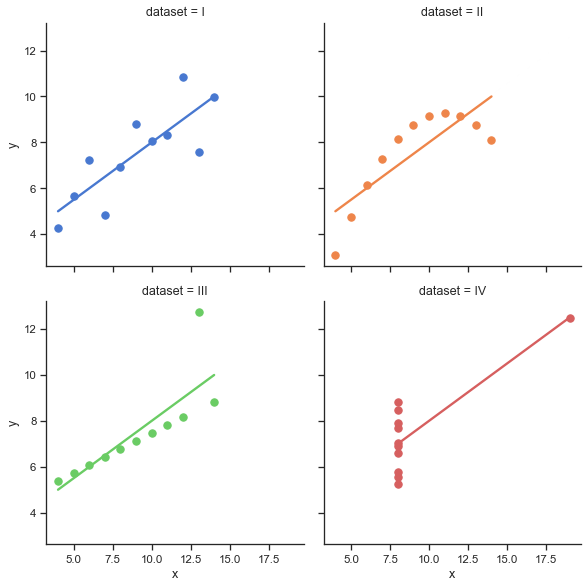
"# [Anscombe's quartet](https://en.wikipedia.org/wiki/Anscombe%27s_quartet)\n",
"\n",
""
]
},
{
"cell_type": "markdown",
"id": "56ec767a",
"metadata": {
"slideshow": {
"slide_type": "slide"
}
},
"source": [
"# Loss functions\n",
"\n",
"The error in a single prediction $f(x_i,c)$ of an observation $(x_i, y_i)$ is often measured as\n",
"$$ \\frac 1 2 \\big( f(x_i, c) - y_i \\big)^2, $$\n",
"which turns out to have a statistical interpretation when the noise is normally distributed.\n",
"It is natural to define the error over the entire data set as\n",
"\\begin{align} L(c; x, y) &= \\sum_i \\frac 1 2 \\big( f(x_i, c) - y_i \\big)^2 \\\\\n",
"&= \\frac 1 2 \\lVert f(x, c) - y \\rVert^2\n",
"\\end{align}\n",
"where I've used the notation $f(x,c)$ to mean the vector resulting from gathering all of the outputs $f(x_i, c)$.\n",
"The function $L$ is called the \"loss function\" and is the key to relaxing the above assumptions."
]
},
{
"cell_type": "markdown",
"id": "abc4b09d",
"metadata": {
"slideshow": {
"slide_type": "slide"
}
},
"source": [
"# Gradient of scalar-valued function\n",
"\n",
"Let's step back from optimization and consider how to differentiate a function of several variables. Let $f(\\boldsymbol x)$ be a function of a vector $\\boldsymbol x$. For example,\n",
"\n",
"$$ f(\\boldsymbol x) = x_1^2 + \\sin(x_2) e^{3x_3} . $$\n",
"\n",
"We can evaluate the **partial derivative** by differentiating with respect to each component $x_i$ separately (holding the others constant), and collect the result in a vector,\n",
"\n",
"\\begin{align}\n",
"\\frac{\\partial f}{\\partial \\boldsymbol x} &= \\begin{bmatrix} \\frac{\\partial f}{\\partial x_1} & \\frac{\\partial f}{\\partial x_2} & \\frac{\\partial f}{\\partial x_3} \\end{bmatrix} \\\\\n",
"&= \\begin{bmatrix} 2 x_1 & \\cos(x_2) e^{3 x_3} & 3 \\sin(x_2) e^{3 x_3} \\end{bmatrix}.\n",
"\\end{align}\n"
]
},
{
"cell_type": "markdown",
"id": "d97a0aca",
"metadata": {
"slideshow": {
"slide_type": "slide"
}
},
"source": [
"# Gradient of vector-valued functions\n",
"\n",
"Now let's consider a vector-valued function $\\boldsymbol f(\\boldsymbol x)$, e.g.,\n",
"\n",
"$$ \\boldsymbol f(\\boldsymbol x) = \\begin{bmatrix} x_1^2 + \\sin(x_2) e^{3x_3} \\\\ x_1 x_2^2 / x_3 \\end{bmatrix} . $$\n",
"\n",
"and write the derivative as a matrix,\n",
"\n",
"\\begin{align}\n",
"\\frac{\\partial \\boldsymbol f}{\\partial \\boldsymbol x} &=\n",
"\\begin{bmatrix} \\frac{\\partial f_1}{\\partial x_1} & \\frac{\\partial f_1}{\\partial x_2} & \\frac{\\partial f_1}{\\partial x_3} \\\\\n",
"\\frac{\\partial f_2}{\\partial x_1} & \\frac{\\partial f_2}{\\partial x_2} & \\frac{\\partial f_2}{\\partial x_3} \\\\\n",
"\\end{bmatrix} \\\\\n",
"&= \\begin{bmatrix} 2 x_1 & \\cos(x_2) e^{3 x_3} & 3 \\sin(x_2) e^{3 x_3} \\\\\n",
"x_2^2 / x_3 & 2 x_1 x_2 / x_3 & -x_1 x_2^2 / x_3^2\n",
"\\end{bmatrix}.\n",
"\\end{align}"
]
},
{
"cell_type": "markdown",
"id": "c1f2648c",
"metadata": {
"slideshow": {
"slide_type": "slide"
}
},
"source": [
"# Geometry of partial derivatives\n",
"\n",
"\n",
"\n",
"* Handy resource on partial derivatives for matrices and vectors: https://explained.ai/matrix-calculus/index.html#sec3"
]
},
{
"cell_type": "markdown",
"id": "05181b72",
"metadata": {
"slideshow": {
"slide_type": "slide"
}
},
"source": [
"# Derivative of a dot product\n",
"\n",
"Let $f(\\boldsymbol x) = \\boldsymbol y^T \\boldsymbol x = \\sum_i y_i x_i$ and compute the derivative\n",
"\n",
"$$ \\frac{\\partial f}{\\partial \\boldsymbol x} = \\begin{bmatrix} y_1 & y_2 & \\dotsb \\end{bmatrix} = \\boldsymbol y^T . $$\n",
"\n",
"Note that $\\boldsymbol y^T \\boldsymbol x = \\boldsymbol x^T \\boldsymbol y$ and we have the product rule,\n",
"\n",
"$$ \\frac{\\partial \\lVert \\boldsymbol x \\rVert^2}{\\partial \\boldsymbol x} = \\frac{\\partial \\boldsymbol x^T \\boldsymbol x}{\\partial \\boldsymbol x} = 2 \\boldsymbol x^T . $$\n",
"\n",
"Also,\n",
"$$ \\frac{\\partial \\lVert \\boldsymbol x - \\boldsymbol y \\rVert^2}{\\partial \\boldsymbol x} = \\frac{\\partial (\\boldsymbol x - \\boldsymbol y)^T (\\boldsymbol x - \\boldsymbol y)}{\\partial \\boldsymbol x} = 2 (\\boldsymbol x - \\boldsymbol y)^T .$$"
]
},
{
"cell_type": "markdown",
"id": "f29e52ed",
"metadata": {
"slideshow": {
"slide_type": "slide"
}
},
"source": [
"# Variational notation\n",
"\n",
"It's convenient to express derivatives in terms of how they act on an infinitessimal perturbation. So we might write\n",
"\n",
"$$ \\delta f = \\frac{\\partial f}{\\partial x} \\delta x .$$\n",
"\n",
"(It's common to use $\\delta x$ or $dx$ for these infinitesimals.) This makes inner products look like a normal product rule\n",
"\n",
"$$ \\delta(\\mathbf x^T \\mathbf y) = (\\delta \\mathbf x)^T \\mathbf y + \\mathbf x^T (\\delta \\mathbf y). $$\n",
"\n",
"A powerful example of variational notation is differentiating a matrix inverse\n",
"\n",
"$$ 0 = \\delta I = \\delta(A^{-1} A) = (\\delta A^{-1}) A + A^{-1} (\\delta A) $$\n",
"and thus\n",
"$$ \\delta A^{-1} = - A^{-1} (\\delta A) A^{-1} $$"
]
},
{
"cell_type": "markdown",
"id": "f5a1c5ad",
"metadata": {
"slideshow": {
"slide_type": "slide"
}
},
"source": [
"# Practice\n",
"\n",
"1. Differentiate $f(x) = A x$ with respect to $x$\n",
"2. Differentiate $f(A) = A x$ with respect to $A$"
]
},
{
"cell_type": "markdown",
"id": "eea01b31",
"metadata": {
"slideshow": {
"slide_type": "slide"
}
},
"source": [
"# Optimization\n",
"Given data $(x,y)$ and loss function $L(c; x,y)$, we wish to find the coefficients $c$ that minimize the loss, thus yielding the \"best predictor\" (in a sense that can be made statistically precise). I.e.,\n",
"$$ \\bar c = \\arg\\min_c L(c; x,y) . $$\n",
"\n",
"It is usually desirable to design models such that the loss function is differentiable with respect to the coefficients $c$, because this allows the use of more efficient optimization methods. Recall that our forward model is given in terms of the Vandermonde matrix,\n",
"\n",
"$$ f(x, c) = V(x) c $$\n",
"\n",
"and thus\n",
"\n",
"$$ \\frac{\\partial f}{\\partial c} = V(x) . $$"
]
},
{
"cell_type": "markdown",
"id": "254b58df",
"metadata": {
"slideshow": {
"slide_type": "slide"
}
},
"source": [
"# Derivative of loss function\n",
"\n",
"We can now differentiate our loss function\n",
"$$ L(c; x, y) = \\frac 1 2 \\lVert f(x, c) - y \\rVert^2 = \\frac 1 2 \\sum_i (f(x_i,c) - y_i)^2 $$\n",
"term-by-term as\n",
"\\begin{align} \\nabla_c L(c; x,y) = \\frac{\\partial L(c; x,y)}{\\partial c} &= \\sum_i \\big( f(x_i, c) - y_i \\big) \\frac{\\partial f(x_i, c)}{\\partial c} \\\\\n",
"&= \\sum_i \\big( f(x_i, c) - y_i \\big) V(x_i)\n",
"\\end{align}\n",
"where $V(x_i)$ is the $i$th row of $V(x)$."
]
},
{
"cell_type": "markdown",
"id": "b7768203",
"metadata": {
"slideshow": {
"slide_type": "slide"
}
},
"source": [
"# Alternative derivative\n",
"Alternatively, we can take a more linear algebraic approach to write the same expression is\n",
"\\begin{align} \\nabla_c L(c; x,y) &= \\big( f(x,c) - y \\big)^T V(x) \\\\\n",
"&= \\big(V(x) c - y \\big)^T V(x) \\\\\n",
"&= V(x)^T \\big( V(x) c - y \\big) .\n",
"\\end{align}\n",
"A necessary condition for the loss function to be minimized is that $\\nabla_c L(c; x,y) = 0$.\n",
"\n",
"* Is the condition sufficient for general $f(x, c)$?\n",
"* Is the condition sufficient for the linear model $f(x,c) = V(x) c$?\n",
"* Have we seen this sort of equation before?"
]
}
],
"metadata": {
"@webio": {
"lastCommId": null,
"lastKernelId": null
},
"celltoolbar": "Slideshow",
"hide_code_all_hidden": false,
"kernelspec": {
"display_name": "Julia 1.7.2",
"language": "julia",
"name": "julia-1.7"
},
"language_info": {
"file_extension": ".jl",
"mimetype": "application/julia",
"name": "julia",
"version": "1.8.5"
},
"rise": {
"enable_chalkboard": true
}
},
"nbformat": 4,
"nbformat_minor": 5
}
 \n",
"\n",
"* Handy resource on partial derivatives for matrices and vectors: https://explained.ai/matrix-calculus/index.html#sec3"
]
},
{
"cell_type": "markdown",
"id": "05181b72",
"metadata": {
"slideshow": {
"slide_type": "slide"
}
},
"source": [
"# Derivative of a dot product\n",
"\n",
"Let $f(\\boldsymbol x) = \\boldsymbol y^T \\boldsymbol x = \\sum_i y_i x_i$ and compute the derivative\n",
"\n",
"$$ \\frac{\\partial f}{\\partial \\boldsymbol x} = \\begin{bmatrix} y_1 & y_2 & \\dotsb \\end{bmatrix} = \\boldsymbol y^T . $$\n",
"\n",
"Note that $\\boldsymbol y^T \\boldsymbol x = \\boldsymbol x^T \\boldsymbol y$ and we have the product rule,\n",
"\n",
"$$ \\frac{\\partial \\lVert \\boldsymbol x \\rVert^2}{\\partial \\boldsymbol x} = \\frac{\\partial \\boldsymbol x^T \\boldsymbol x}{\\partial \\boldsymbol x} = 2 \\boldsymbol x^T . $$\n",
"\n",
"Also,\n",
"$$ \\frac{\\partial \\lVert \\boldsymbol x - \\boldsymbol y \\rVert^2}{\\partial \\boldsymbol x} = \\frac{\\partial (\\boldsymbol x - \\boldsymbol y)^T (\\boldsymbol x - \\boldsymbol y)}{\\partial \\boldsymbol x} = 2 (\\boldsymbol x - \\boldsymbol y)^T .$$"
]
},
{
"cell_type": "markdown",
"id": "f29e52ed",
"metadata": {
"slideshow": {
"slide_type": "slide"
}
},
"source": [
"# Variational notation\n",
"\n",
"It's convenient to express derivatives in terms of how they act on an infinitessimal perturbation. So we might write\n",
"\n",
"$$ \\delta f = \\frac{\\partial f}{\\partial x} \\delta x .$$\n",
"\n",
"(It's common to use $\\delta x$ or $dx$ for these infinitesimals.) This makes inner products look like a normal product rule\n",
"\n",
"$$ \\delta(\\mathbf x^T \\mathbf y) = (\\delta \\mathbf x)^T \\mathbf y + \\mathbf x^T (\\delta \\mathbf y). $$\n",
"\n",
"A powerful example of variational notation is differentiating a matrix inverse\n",
"\n",
"$$ 0 = \\delta I = \\delta(A^{-1} A) = (\\delta A^{-1}) A + A^{-1} (\\delta A) $$\n",
"and thus\n",
"$$ \\delta A^{-1} = - A^{-1} (\\delta A) A^{-1} $$"
]
},
{
"cell_type": "markdown",
"id": "f5a1c5ad",
"metadata": {
"slideshow": {
"slide_type": "slide"
}
},
"source": [
"# Practice\n",
"\n",
"1. Differentiate $f(x) = A x$ with respect to $x$\n",
"2. Differentiate $f(A) = A x$ with respect to $A$"
]
},
{
"cell_type": "markdown",
"id": "eea01b31",
"metadata": {
"slideshow": {
"slide_type": "slide"
}
},
"source": [
"# Optimization\n",
"Given data $(x,y)$ and loss function $L(c; x,y)$, we wish to find the coefficients $c$ that minimize the loss, thus yielding the \"best predictor\" (in a sense that can be made statistically precise). I.e.,\n",
"$$ \\bar c = \\arg\\min_c L(c; x,y) . $$\n",
"\n",
"It is usually desirable to design models such that the loss function is differentiable with respect to the coefficients $c$, because this allows the use of more efficient optimization methods. Recall that our forward model is given in terms of the Vandermonde matrix,\n",
"\n",
"$$ f(x, c) = V(x) c $$\n",
"\n",
"and thus\n",
"\n",
"$$ \\frac{\\partial f}{\\partial c} = V(x) . $$"
]
},
{
"cell_type": "markdown",
"id": "254b58df",
"metadata": {
"slideshow": {
"slide_type": "slide"
}
},
"source": [
"# Derivative of loss function\n",
"\n",
"We can now differentiate our loss function\n",
"$$ L(c; x, y) = \\frac 1 2 \\lVert f(x, c) - y \\rVert^2 = \\frac 1 2 \\sum_i (f(x_i,c) - y_i)^2 $$\n",
"term-by-term as\n",
"\\begin{align} \\nabla_c L(c; x,y) = \\frac{\\partial L(c; x,y)}{\\partial c} &= \\sum_i \\big( f(x_i, c) - y_i \\big) \\frac{\\partial f(x_i, c)}{\\partial c} \\\\\n",
"&= \\sum_i \\big( f(x_i, c) - y_i \\big) V(x_i)\n",
"\\end{align}\n",
"where $V(x_i)$ is the $i$th row of $V(x)$."
]
},
{
"cell_type": "markdown",
"id": "b7768203",
"metadata": {
"slideshow": {
"slide_type": "slide"
}
},
"source": [
"# Alternative derivative\n",
"Alternatively, we can take a more linear algebraic approach to write the same expression is\n",
"\\begin{align} \\nabla_c L(c; x,y) &= \\big( f(x,c) - y \\big)^T V(x) \\\\\n",
"&= \\big(V(x) c - y \\big)^T V(x) \\\\\n",
"&= V(x)^T \\big( V(x) c - y \\big) .\n",
"\\end{align}\n",
"A necessary condition for the loss function to be minimized is that $\\nabla_c L(c; x,y) = 0$.\n",
"\n",
"* Is the condition sufficient for general $f(x, c)$?\n",
"* Is the condition sufficient for the linear model $f(x,c) = V(x) c$?\n",
"* Have we seen this sort of equation before?"
]
}
],
"metadata": {
"@webio": {
"lastCommId": null,
"lastKernelId": null
},
"celltoolbar": "Slideshow",
"hide_code_all_hidden": false,
"kernelspec": {
"display_name": "Julia 1.7.2",
"language": "julia",
"name": "julia-1.7"
},
"language_info": {
"file_extension": ".jl",
"mimetype": "application/julia",
"name": "julia",
"version": "1.8.5"
},
"rise": {
"enable_chalkboard": true
}
},
"nbformat": 4,
"nbformat_minor": 5
}
\n",
"\n",
"* Handy resource on partial derivatives for matrices and vectors: https://explained.ai/matrix-calculus/index.html#sec3"
]
},
{
"cell_type": "markdown",
"id": "05181b72",
"metadata": {
"slideshow": {
"slide_type": "slide"
}
},
"source": [
"# Derivative of a dot product\n",
"\n",
"Let $f(\\boldsymbol x) = \\boldsymbol y^T \\boldsymbol x = \\sum_i y_i x_i$ and compute the derivative\n",
"\n",
"$$ \\frac{\\partial f}{\\partial \\boldsymbol x} = \\begin{bmatrix} y_1 & y_2 & \\dotsb \\end{bmatrix} = \\boldsymbol y^T . $$\n",
"\n",
"Note that $\\boldsymbol y^T \\boldsymbol x = \\boldsymbol x^T \\boldsymbol y$ and we have the product rule,\n",
"\n",
"$$ \\frac{\\partial \\lVert \\boldsymbol x \\rVert^2}{\\partial \\boldsymbol x} = \\frac{\\partial \\boldsymbol x^T \\boldsymbol x}{\\partial \\boldsymbol x} = 2 \\boldsymbol x^T . $$\n",
"\n",
"Also,\n",
"$$ \\frac{\\partial \\lVert \\boldsymbol x - \\boldsymbol y \\rVert^2}{\\partial \\boldsymbol x} = \\frac{\\partial (\\boldsymbol x - \\boldsymbol y)^T (\\boldsymbol x - \\boldsymbol y)}{\\partial \\boldsymbol x} = 2 (\\boldsymbol x - \\boldsymbol y)^T .$$"
]
},
{
"cell_type": "markdown",
"id": "f29e52ed",
"metadata": {
"slideshow": {
"slide_type": "slide"
}
},
"source": [
"# Variational notation\n",
"\n",
"It's convenient to express derivatives in terms of how they act on an infinitessimal perturbation. So we might write\n",
"\n",
"$$ \\delta f = \\frac{\\partial f}{\\partial x} \\delta x .$$\n",
"\n",
"(It's common to use $\\delta x$ or $dx$ for these infinitesimals.) This makes inner products look like a normal product rule\n",
"\n",
"$$ \\delta(\\mathbf x^T \\mathbf y) = (\\delta \\mathbf x)^T \\mathbf y + \\mathbf x^T (\\delta \\mathbf y). $$\n",
"\n",
"A powerful example of variational notation is differentiating a matrix inverse\n",
"\n",
"$$ 0 = \\delta I = \\delta(A^{-1} A) = (\\delta A^{-1}) A + A^{-1} (\\delta A) $$\n",
"and thus\n",
"$$ \\delta A^{-1} = - A^{-1} (\\delta A) A^{-1} $$"
]
},
{
"cell_type": "markdown",
"id": "f5a1c5ad",
"metadata": {
"slideshow": {
"slide_type": "slide"
}
},
"source": [
"# Practice\n",
"\n",
"1. Differentiate $f(x) = A x$ with respect to $x$\n",
"2. Differentiate $f(A) = A x$ with respect to $A$"
]
},
{
"cell_type": "markdown",
"id": "eea01b31",
"metadata": {
"slideshow": {
"slide_type": "slide"
}
},
"source": [
"# Optimization\n",
"Given data $(x,y)$ and loss function $L(c; x,y)$, we wish to find the coefficients $c$ that minimize the loss, thus yielding the \"best predictor\" (in a sense that can be made statistically precise). I.e.,\n",
"$$ \\bar c = \\arg\\min_c L(c; x,y) . $$\n",
"\n",
"It is usually desirable to design models such that the loss function is differentiable with respect to the coefficients $c$, because this allows the use of more efficient optimization methods. Recall that our forward model is given in terms of the Vandermonde matrix,\n",
"\n",
"$$ f(x, c) = V(x) c $$\n",
"\n",
"and thus\n",
"\n",
"$$ \\frac{\\partial f}{\\partial c} = V(x) . $$"
]
},
{
"cell_type": "markdown",
"id": "254b58df",
"metadata": {
"slideshow": {
"slide_type": "slide"
}
},
"source": [
"# Derivative of loss function\n",
"\n",
"We can now differentiate our loss function\n",
"$$ L(c; x, y) = \\frac 1 2 \\lVert f(x, c) - y \\rVert^2 = \\frac 1 2 \\sum_i (f(x_i,c) - y_i)^2 $$\n",
"term-by-term as\n",
"\\begin{align} \\nabla_c L(c; x,y) = \\frac{\\partial L(c; x,y)}{\\partial c} &= \\sum_i \\big( f(x_i, c) - y_i \\big) \\frac{\\partial f(x_i, c)}{\\partial c} \\\\\n",
"&= \\sum_i \\big( f(x_i, c) - y_i \\big) V(x_i)\n",
"\\end{align}\n",
"where $V(x_i)$ is the $i$th row of $V(x)$."
]
},
{
"cell_type": "markdown",
"id": "b7768203",
"metadata": {
"slideshow": {
"slide_type": "slide"
}
},
"source": [
"# Alternative derivative\n",
"Alternatively, we can take a more linear algebraic approach to write the same expression is\n",
"\\begin{align} \\nabla_c L(c; x,y) &= \\big( f(x,c) - y \\big)^T V(x) \\\\\n",
"&= \\big(V(x) c - y \\big)^T V(x) \\\\\n",
"&= V(x)^T \\big( V(x) c - y \\big) .\n",
"\\end{align}\n",
"A necessary condition for the loss function to be minimized is that $\\nabla_c L(c; x,y) = 0$.\n",
"\n",
"* Is the condition sufficient for general $f(x, c)$?\n",
"* Is the condition sufficient for the linear model $f(x,c) = V(x) c$?\n",
"* Have we seen this sort of equation before?"
]
}
],
"metadata": {
"@webio": {
"lastCommId": null,
"lastKernelId": null
},
"celltoolbar": "Slideshow",
"hide_code_all_hidden": false,
"kernelspec": {
"display_name": "Julia 1.7.2",
"language": "julia",
"name": "julia-1.7"
},
"language_info": {
"file_extension": ".jl",
"mimetype": "application/julia",
"name": "julia",
"version": "1.8.5"
},
"rise": {
"enable_chalkboard": true
}
},
"nbformat": 4,
"nbformat_minor": 5
}