Example 1 Overview

GLMsingle is new tool that provides efficient, scalable, and accurate single-trial fMRI response estimates.

The purpose of this Example 1 notebook is to guide the user through basic calls to GLMsingle, using a representative, small-scale test dataset (in this case, an example session from a rapid event-related visual fMRI dataset - the Natural Scenes Dataset core experiment).

The goal is to examine the effect of GLMsingle on the reliability of single-trial fMRI response estimates. By default, the tool implements a set of optimizations that improve upon generic GLM approaches by: (1) identifying an optimal hemodynamic response function (HRF) at each voxel, (2) deriving a set of useful GLM nuisance regressors via "GLMdenoise" and picking an optimal number to include in the final GLM, and (3) applying a custom amount of ridge regularization at each voxel using an efficient technique called "fracridge". The output of GLMsingle are GLM betas reflecting the estimated percent signal change in each voxel in response to each experimental stimulus or condition being modeled.

Beyond directly improving the reliability of neural responses to repeated stimuli, these optimized techniques for signal estimation can have a range of desirable downstream effects such as: improving cross-subject representational similarity within and between datasets; improving the single-image decodability of evoked neural patterns via MVPA; and, decreasing the correlation in spatial patterns observed at neighboring timepoints in analysis of fMRI GLM outputs. See our video presentation at V-VSS 2020 for a summary of these phenomena as observed in recent massive-scale fMRI datasets (the Natural Scenes Dataset and BOLD5000): https://www.youtube.com/watch?v=yb3Nn7Han8o

Example 1 contains a full walkthrough of the process of loading an example dataset and design matrix, estimating neural responses using GLMsingle, estimating the reliability of responses at each voxel, and comparing those achieved via GLMsingle to those achieved using a baseline GLM. After loading and visualizing formatted fMRI time-series and their corresponding design matrices, we will describe the default behavior of GLMsingle and show how to modify hyperparameters if the user desires. Throughout the notebook we will highlight important metrics and outputs using figures, print statements, and comments.

Users encountering bugs, unexpected outputs, or other issues regarding GLMsingle shouldn't hesitate to raise an issue on GitHub: https://github.com/kendrickkay/GLMsingle/issues

Add dependencies and download the example dataset
Data overview
Call GLMestimatesingletrial with default parameters
Summary of important outputs
Plot a slice of brain showing GLMsingle outputs
Run a baseline GLM to compare with GLMsingle
Get indices of repeated conditions to use for reliability calculations
Compute median split-half reliability for each GLM version
Compare visual voxel reliabilities between beta versions

Add dependencies and download the example dataset

% We will assume that the current working directory is the directory that
% contains this script.

% Add path to GLMsingle
addpath(genpath('../../matlab'));

% You also need fracridge repository to run this code. For example, you
% could do:
%   git clone https://github.com/nrdg/fracridge.git
% and then do:
%   addpath('fracridge')

% Start fresh
clear
clc
close all

% Name of directory to which outputs will be saved
outputdir = 'example1outputs';

% Download files to data directory
if ~exist('./data','dir')
    mkdir('data')
end

if ~exist('./data/nsdcoreexampledataset.mat','file')
    % download data with curl
    system('curl -L --output ./data/nsdcoreexampledataset.mat https://osf.io/k89b2/download')
end
load('./data/nsdcoreexampledataset.mat')
% Data comes from the NSD dataset (subj01, nsd01 scan session).
% https://www.biorxiv.org/content/10.1101/2021.02.22.432340v1.full.pdf

Data overview

clc
whos

% data -> consists of several runs of 4D volume files (x,y,z,t)  where
% (t)ime is the 4th dimention. In this example, data consists of only a
% single slice and has been prepared with a TR = 1s

% ROI -> manually defined region in the occipital cortex. It is a binary
% matrix where (x,y,z) = 1 corresponds to the cortical area that responded
% to visual stimuli used in the NSD project.

fprintf('There are %d runs in total.\n',length(design));
fprintf('The dimensions of the data for the first run are %s.\n',mat2str(size(data{1})));
fprintf('The stimulus duration is %.3f seconds.\n',stimdur);
fprintf('The sampling rate (TR) is %.3f seconds.\n',tr);

  Name             Size                 Bytes  Class     Attributes

  ROI            145x186               215760  double              
  data             1x12             388369344  cell                
  design           1x12                 69408  cell                
  outputdir        1x15                    30  char                
  stimdur          1x1                      8  double              
  tr               1x1                      8  double              

There are 12 runs in total.
The dimensions of the data for the first run are [145 186 1 300].
The stimulus duration is 3.000 seconds.
The sampling rate (TR) is 1.000 seconds.

figure(1);clf

%Show example design matrix.
for d = 1
    imagesc(design{d}); colormap gray; drawnow
    xlabel('Conditions')
    ylabel('TRs')
    title(sprintf('Design matrix for run%i',d))
    axis image
end

xticks(0:53:length(design{d}))
set(gcf,'Position',[418   412   782   605])

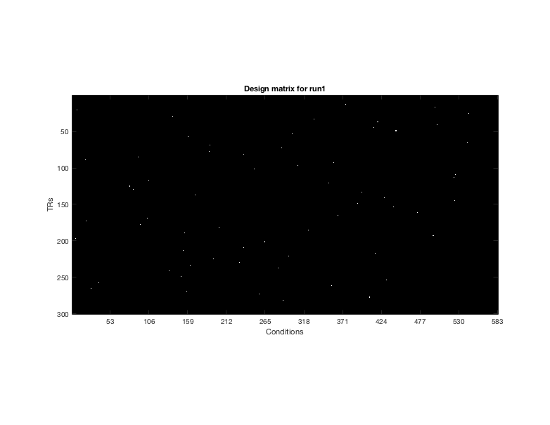
design -> Each run has a corresponding design matrix where each column describes a single condition (conditions are repeated across runs). Each design matrix is binary with 1 specfing the time (TR) when the stimulus is presented on the screen.

In this NSD scan session, there are a total of 750 trials, in which a total of 583 distinct images are shown. (Thus, some images were presented more than once.) In the design matrix shown, there are 583 predictor columns/conditions, one per distinct image. Notice that white rectangles are pseudo randomized and they indicate when the presentation of each image occurs. Note that in some runs not all images are shown; if a column does not have a white rectangle it means that this image is shown in a different run within the session.

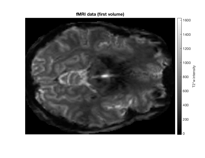
% Show an example slice of the first fMRI volume.
figure(2);clf
imagesc(data{1}(:,:,:,1));
colormap(gray);
axis equal tight;
c=colorbar;
title('fMRI data (first volume)');
set(gcf,'Position',[418   412   782   605])
axis off
c.Label.String = 'T2*w intensity';
set(gca,'FontSize',15)

Call GLMestimatesingletrial with default parameters

% Outputs and figures will be stored in a folder (you can specify its name
% as the 5th input to GLMestimatesingletrial). Model estimates can be also
% saved to the 'results' variable which is the only output of
% GLMestimatesingletrial.

% Optional parameters below can be assigned to a structure, i.e., opt =
% struct('wantlibrary',1,'wantglmdenoise',1); Options are the 6th input to
% GLMestimatesingletrial.

% There are many options that can be specified; here, we comment on the
% main options that one might want to modify/set. Defaults for the options
% are indicated below.

% wantlibrary = 1 -> Fit HRF to each voxel
% wantglmdenoise = 1 -> Use GLMdenoise
% wantfracridge = 1  -> Use ridge regression to improve beta estimates
% chunknum = 50000 -> is the number of voxels that we will
%     process at the same time. For setups with lower memory, you may need to
%     decrease this number.

% wantmemoryoutputs is a logical vector [A B C D] indicating which of the
%     four model types to return in the output <results>. The user must be
%     careful with this, as large datasets can require a lot of RAM. If you
%     do not request the various model types, they will be cleared from
%     memory (but still potentially saved to disk). Default: [0 0 0 1]
%     which means return only the final type-D model.

% wantfileoutputs is a logical vector [A B C D] indicating which of the
%     four model types to save to disk (assuming that they are computed). A
%     = 0/1 for saving the results of the ONOFF model, B = 0/1 for saving
%     the results of the FITHRF model, C = 0/1 for saving the results of the
%     FITHRF_GLMdenoise model, D = 0/1 for saving the results of the
%     FITHRF_GLMdenoise_RR model. Default: [1 1 1 1] which means save all
%     computed results to disk.

% numpcstotry (optional) is a non-negative integer indicating the maximum
%     number of GLMdenoise PCs to enter into the model. Default: 10.

% fracs (optional) is a vector of fractions that are greater than 0
%     and less than or equal to 1. We automatically sort in descending
%     order and ensure the fractions are unique. These fractions indicate
%     the regularization levels to evaluate using fractional ridge
%     regression (fracridge) and cross-validation. Default:
%     fliplr(.05:.05:1). A special case is when <fracs> is specified as a
%     single scalar value. In this case, cross-validation is NOT performed
%     for the type-D model, and we instead blindly use the supplied
%     fractional value for the type-D model.

% For the purpose of this example, we will keep all outputs in the memory.
opt = struct('wantmemoryoutputs',[1 1 1 1]);

% This example saves output .mat files to the folder
% "example1outputs/GLMsingle". If these outputs don't already exist, we
% will perform the time-consuming call to GLMestimatesingletrial.m;
% otherwise, we will just load from disk.
if ~exist([outputdir '/GLMsingle'],'dir')

    [results] = GLMestimatesingletrial(design,data,stimdur,tr,[outputdir '/GLMsingle'],opt);

    % We assign outputs of GLMestimatesingletrial to "models" structure.
    % Note that results{1} contains GLM estimates from an ONOFF model,
    % where all images are treated as the same condition. These estimates
    % could be potentially used to find cortical areas that respond to
    % visual stimuli. We want to compare beta weights between conditions
    % therefore we are not going to store the ONOFF GLM results.

    clear models;
    models.FIT_HRF = results{2};
    models.FIT_HRF_GLMdenoise = results{3};
    models.FIT_HRF_GLMdenoise_RR = results{4};

else
    % Load existing file outputs if they exist
    results = load([outputdir '/GLMsingle/TYPEB_FITHRF.mat']);
    models.FIT_HRF = results;
    results = load([outputdir '/GLMsingle/TYPEC_FITHRF_GLMDENOISE.mat']);
    models.FIT_HRF_GLMdenoise = results;
    results = load([outputdir '/GLMsingle/TYPED_FITHRF_GLMDENOISE_RR.mat']);
    models.FIT_HRF_GLMdenoise_RR = results;

end

Summary of important outputs

% The outputs of GLMestimatesingletrial.m are formally documented in its
% header. Here, we highlight a few of the more important outputs:
%
% R2 -> is model accuracy expressed in terms of R^2 (percentage).
%
% modelmd -> is the full set of single-trial beta weights (X x Y x Z x
% TRIALS). Beta weights are arranged in chronological order.
%
% HRFindex -> is the 1-index of the best fit HRF. HRFs can be recovered
% with getcanonicalHRFlibrary(stimdur,tr)
%
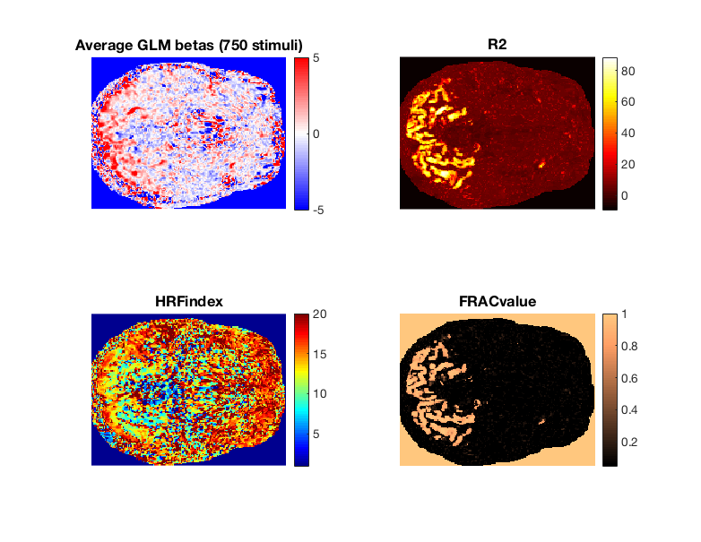
% FRACvalue -> is the fractional ridge regression regularization level
% chosen for each voxel. Values closer to 1 mean less regularization.

Plot a slice of brain showing GLMsingle outputs

% We are going to plot several outputs from the FIT_HRF_GLMdenoise_RR GLM,
% which contains the full set of GLMsingle optimizations.

slice = 1;

% we will plot betas, R2, optimal HRF indices, and the voxel frac values
val2plot = {'modelmd';'R2';'HRFindex';'FRACvalue'};
cmaps = {cmapsign2;hot;jet;copper};

figure(3);clf

for v = 1 : length(val2plot)

    f=subplot(2,2,v);

    if contains('modelmd',val2plot{v})
        % When plotting betas, for simplicity just average across all image
        % presentations This will yield a summary of whether voxels tend to
        % increase or decrease their activity in response to the
        % experimental stimuli (similar to outputs from an ONOFF GLM)
        imagesc(nanmean(models.FIT_HRF_GLMdenoise_RR.(val2plot{v})(:,:,slice),4),[-5 5]); axis off image;
        title('Average GLM betas (750 stimuli)')

    else
        % Plot all other voxel-wise metrics as outputted from GLMsingle
        imagesc(models.FIT_HRF_GLMdenoise_RR.(val2plot{v})(:,:,slice)); axis off image;
        title(val2plot{v})

    end

    colormap(f,cmaps{v})
    colorbar
    set(gca,'FontSize',15)
end

set(gcf,'Position',[418   412   782   605])

Run a baseline GLM to compare with GLMsingle

% Additionally, for comparison purposes we are going to run a standard GLM
% without HRF fitting, GLMdenoise, or ridge regression regularization. We
% will change the default settings by using the "opt" structure.
opt.wantlibrary = 0; % switch off HRF fitting
opt.wantglmdenoise = 0; % switch off GLMdenoise
opt.wantfracridge = 0; % switch off ridge regression
opt.wantfileoutputs = [0 1 0 0];
opt.wantmemoryoutputs = [0 1 0 0];

% If these outputs don't already exist, we will perform the call to
% GLMestimatesingletrial.m; otherwise, we will just load from disk.
if ~exist([outputdir '/GLMbaseline'],'dir')

    [ASSUME_HRF] = GLMestimatesingletrial(design,data,stimdur,tr,[outputdir '/GLMbaseline'],opt);
    models.ASSUME_HRF = ASSUME_HRF{2};

else

    % Note that even though we are loading TYPEB_FITHRF betas, HRF fitting
    % has been turned off and this struct field will thus contain the
    % outputs of a GLM fit using the canonical HRF.
    results = load([outputdir '/GLMbaseline/TYPEB_FITHRF.mat']);
    models.ASSUME_HRF = results;

end

% We assign outputs from GLMestimatesingletrial to "models" structure.
% Again, results{1} contains GLM estimates from an ONOFF model so we are
% not going to extract it.

% Now, "models" variable holds solutions for 4 GLM models
disp(fieldnames(models))

    'FIT_HRF'
    'FIT_HRF_GLMdenoise'
    'FIT_HRF_GLMdenoise_RR'
    'ASSUME_HRF'

Get indices of repeated conditions to use for reliability calculations

% To compare the results of different GLMs we are going to calculate the
% voxel-wise split-half reliablity for each model. Reliability values
% reflect a correlation between beta weights for repeated presentations of
% the same conditions. In short, we are going to check how
% reliable/reproducible are the single trial responses to repeated
% conditions estimated with each GLM type.

% This NSD scan session has a large number of images that are just shown
% once during the session, some images that are shown twice, and a few that
% are shown three times. In the code below, we are attempting to locate the
% indices in the beta weight GLMsingle outputs modelmd(x,y,z,trials) that
% correspond to repeated images. Here we only consider stimuli that have
% been presented at least twice. For the purpose of the example we ignore
% the 3rd repetition of the stimulus.

% Consolidate design matrices
designALL = cat(1,design{:});

% Construct a vector containing 1-indexed condition numbers in
% chronological order.

corder = [];
for p=1:size(designALL,1)
    if any(designALL(p,:))
        corder = [corder find(designALL(p,:))];
    end
end

% Let's take a look at the first few entries
corder(1:3)

% Note that [375 497 8] means that the first stimulus trial involved
% presentation of the 375th condition, the second stimulus trial involved
% presentation of the 497th condition, and so on.

ans =

   375   497     8

% In order to compute split-half reliability, we have to do some indexing.
% we want to find images with least two repetitions and then prepare a
% useful matrix of indices that refer to when these occur.
repindices = [];  % 2 x images containing stimulus trial indices.

% The first row refers to the first presentation; the second row refers to
% the second presentation.
for p=1:size(designALL,2)  % loop over every condition
    temp = find(corder==p);
    if length(temp) >= 2
        repindices = cat(2,repindices,[temp(1); temp(2)]);  % note that for images with 3 presentations, we are simply ignoring the third trial
    end
end

% Let's take a look at a few entries
repindices(:,1:3)

% Notice that the first condition is presented on the 217th stimulus trial
% and the 486th stimulus trial, the second condition is presented on the
% 218th and 621st stimulus trials, and so on.

fprintf('There are %i repeated images in the experiment \n',length(repindices))

% Now, for each voxel we are going to correlate beta weights describing the
% response to images presented for the first time with beta weights
% describing the response from the repetition of the same image. With 136
% repeated conditions, the correlation for each voxel will reflect the
% relationship between two vectors with 136 beta weights each.

ans =

   217   218    19
   486   621   124

There are 136 repeated images in the experiment

Compute median split-half reliability for each GLM version

% Finally, let's compute split-half reliability. We are going to loop
% through our 4 models and calculate split-half reliability for each of
% them.

% We first arrange models from least to most sophisticated (for
% visualization purposes)
model_names = fieldnames(models);
model_names = model_names([4 1 2 3]);

% Create output variable for reliability values
vox_reliabilities = cell(1,length(models));

% For each GLM...
for m = 1 : length(model_names)

    % Get the GLM betas
    betas = models.(model_names{m}).modelmd(:,:,:,repindices);  % use indexing to pull out the trials we want
    betas_reshaped = reshape(betas,size(betas,1),size(betas,2),size(betas,3),2,[]);  % reshape to X x Y x Z x 2 x CONDITIONS

    % compute reliabilities using an efficient (vectorized) utility
    % function
    vox_reliabilities{m} = calccorrelation(betas_reshaped(:,:,:,1,:),betas_reshaped(:,:,:,2,:),5);

    % Note that calccorrelation.m is a utility function that computes
    % correlations in a vectorized fashion (for optimal speed).

end

Compare visual voxel reliabilities between beta versions

figure(4);clf
subplot(1,2,1);
cmap = [0.2314    0.6039    0.6980
    0.8615    0.7890    0.2457
    0.8824    0.6863         0
    0.9490    0.1020         0];

% For each GLM type we calculate median reliability for voxels within the
% visual ROI and plot it as a bar plot.
for m = 1 : 4
    bar(m,nanmedian(vox_reliabilities{m}(ROI==1)),'FaceColor','None','Linewidth',3,'EdgeColor',cmap(m,:)); hold on
end
ylabel('Median reliability')
legend(model_names,'Interpreter','None','Location','NorthWest')
set(gca,'Fontsize',16)
set(gca,'TickLabelInterpreter','none')
xtickangle(0)
xticks([])
ylim([0.1 0.2])
set(gcf,'Position',[418   412   782   605])
title('Median voxel split-half reliability of GLM models')

subplot(1,2,1);

% Comparison is the final output (FIT_HRF_GLMDENOISE_RR) vs. the baseline
% GLM (ASSUME_HRF)
vox_reliability = vox_reliabilities{4} - vox_reliabilities{1};
underlay = data{1}(:,:,:,1);
ROI(ROI~=1) = NaN;
overlay = vox_reliability;

underlay_im = cmaplookup(underlay,min(underlay(:)),max(underlay(:)),[],gray(256));
overlay_im = cmaplookup(overlay,-0.3,0.3,[],cmapsign2);

mask = ROI==1;

subplot(1,2,2);
hold on
imagesc(underlay_im);
imagesc(overlay_im, 'AlphaData', mask);
hold off
axis image
colormap(cmapsign2)
c = colorbar;
c.Ticks = [0 0.5 1];
c.TickLabels = {'-0.3';'0';'0.3'};
title('change in nsdgeneral voxel reliability** due to GLMsingle (\Delta{\itr})')
set(gca,'Fontsize',16)
xlabel('**plotting (FITHRF_GLMDENOISE_RR - ASSUMEHRF) reliabilities','Interpreter','none','FontSize',12);
xticks([])
yticks([])

set(gcf,'Position',[36 343 1116 674])

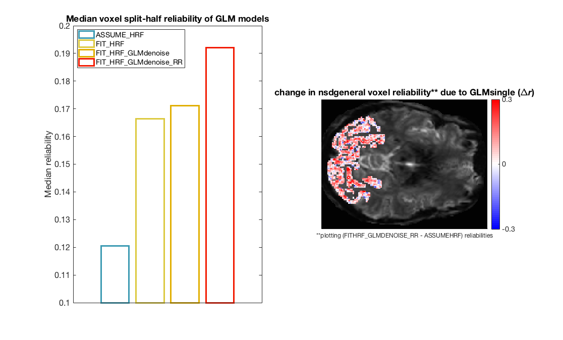
% Notice that there is systematic increase in reliability moving from the
% first to the second to the third to the final fourth version of the GLM
% results. These increases reflect, respectively, the addition of HRF
% fitting, the derivation and use of data-driven nuisance regressors, and
% the use of ridge regression as a way to regularize the instability of
% closely spaced experimental trials. Depending on one's experimental
% goals, it is possible with setting of option flags to activate a subset
% of these analysis features.
%
% Also, keep in mind that in the above figure, we are simply showing the
% median as a metric of the central tendency (you may want to peruse
% individual voxels in scatter plots, for example).