Data analysis on Movies Dataset

by Deepak Das

The main aim of the project is to find insights about the datset containing information about particular movies. This project uses the movie dataset avaliable form Movie lens.This dataset contains just 1000 movies for analysis. We have used libraries present in Python such as Matplotlib,Seaborn,Pandas for reading and visualization of the dataset.

mov

We import the packages required for visualization

In [81]:
import pandas as pd
import matplotlib.pyplot as plt
import seaborn as sns
%matplotlib inline

Data description

The data is in csv format.In computing, a comma-separated values (CSV) file stores tabular data (numbers and text) in plain text. Each line of the file is a data record. Each record consists of one or more fields, separated by commas. Data are collected on 12 different informations of a movie,with rating being in the order of 1 (worst) and 10 (best) and the metascore being in the order from 1 (worst) and 100 (best).

In [82]:
df = pd.read_csv('Documents//movie.csv')

Attributes

  • Rank
  • Title
  • Genre
  • Description
  • Director
  • Actors
  • Year
  • Runtime
  • Rating
  • Votes
  • Revenue
  • Metascore

Here we call the head function and print the first 5 rows of the data

In [28]:
df.head()
Out[28]:
Rank Title Genre Description Director Actors Year Runtime (Minutes) Rating Votes Revenue (Millions) Metascore
0 1 Guardians of the Galaxy Action,Adventure,Sci-Fi A group of intergalactic criminals are forced ... James Gunn Chris Pratt, Vin Diesel, Bradley Cooper, Zoe S... 2014 121 8.1 757074 333.13 76.0
1 2 Prometheus Adventure,Mystery,Sci-Fi Following clues to the origin of mankind, a te... Ridley Scott Noomi Rapace, Logan Marshall-Green, Michael Fa... 2012 124 7.0 485820 126.46 65.0
2 3 Split Horror,Thriller Three girls are kidnapped by a man with a diag... M. Night Shyamalan James McAvoy, Anya Taylor-Joy, Haley Lu Richar... 2016 117 7.3 157606 138.12 62.0
3 4 Sing Animation,Comedy,Family In a city of humanoid animals, a hustling thea... Christophe Lourdelet Matthew McConaughey,Reese Witherspoon, Seth Ma... 2016 108 7.2 60545 270.32 59.0
4 5 Suicide Squad Action,Adventure,Fantasy A secret government agency recruits some of th... David Ayer Will Smith, Jared Leto, Margot Robbie, Viola D... 2016 123 6.2 393727 325.02 40.0

Here we see the total size of the dataset

In [29]:
df.size
Out[29]:
12000

Here we see the shape of the dataset

In [30]:
df.shape
Out[30]:
(1000, 12)

Here we see all the mathematical aspects of the data

In [31]:
df.describe(include = 'all')
Out[31]:
Rank Title Genre Description Director Actors Year Runtime (Minutes) Rating Votes Revenue (Millions) Metascore
count 1000.000000 1000 1000 1000 1000 1000 1000.000000 1000.000000 1000.000000 1.000000e+03 872.000000 936.000000
unique NaN 999 207 1000 644 996 NaN NaN NaN NaN NaN NaN
top NaN The Host Action,Adventure,Sci-Fi Col. Katherine Powell, a military officer in c... Ridley Scott Shia LaBeouf, Megan Fox, Josh Duhamel, Tyrese ... NaN NaN NaN NaN NaN NaN
freq NaN 2 50 1 8 2 NaN NaN NaN NaN NaN NaN
mean 500.500000 NaN NaN NaN NaN NaN 2012.783000 113.172000 6.723200 1.698083e+05 82.956376 58.985043
std 288.819436 NaN NaN NaN NaN NaN 3.205962 18.810908 0.945429 1.887626e+05 103.253540 17.194757
min 1.000000 NaN NaN NaN NaN NaN 2006.000000 66.000000 1.900000 6.100000e+01 0.000000 11.000000
25% 250.750000 NaN NaN NaN NaN NaN 2010.000000 100.000000 6.200000 3.630900e+04 13.270000 47.000000
50% 500.500000 NaN NaN NaN NaN NaN 2014.000000 111.000000 6.800000 1.107990e+05 47.985000 59.500000
75% 750.250000 NaN NaN NaN NaN NaN 2016.000000 123.000000 7.400000 2.399098e+05 113.715000 72.000000
max 1000.000000 NaN NaN NaN NaN NaN 2016.000000 191.000000 9.000000 1.791916e+06 936.630000 100.000000

We check for the missing values in the dataset

We find there are missing values present in the dataset so we will remove the missing values

In [32]:
df.isnull().sum()
Out[32]:
Rank                    0
Title                   0
Genre                   0
Description             0
Director                0
Actors                  0
Year                    0
Runtime (Minutes)       0
Rating                  0
Votes                   0
Revenue (Millions)    128
Metascore              64
dtype: int64

We fill the null values with the mean values in the dataset

In [33]:
df.mean()
Out[33]:
Rank                     500.500000
Year                    2012.783000
Runtime (Minutes)        113.172000
Rating                     6.723200
Votes                 169808.255000
Revenue (Millions)        82.956376
Metascore                 58.985043
dtype: float64

Filling the Null values of the Revenue column with mean values

In [293]:
df['Revenue (Millions)'] = df['Revenue (Millions)'].fillna(df['Revenue (Millions)'].mean())

Filling the Null values of the Metascore column with mean values

In [234]:
df['Metascore'] = df['Metascore'].fillna(df['Metascore'].mean())
In [235]:
df.isnull().sum()
Out[235]:
Rank                  0
Title                 0
Genre                 0
Description           0
Director              0
Actors                0
Year                  0
Runtime (Minutes)     0
Rating                0
Votes                 0
Revenue (Millions)    0
Metascore             0
dtype: int64

We drop the columns which are not required for analysis and for the Recommendation engine

In [236]:
df1 = df.drop(columns = ['Description' ,'Director','Actors'])
df1.head()
Out[236]:
Rank Title Genre Year Runtime (Minutes) Rating Votes Revenue (Millions) Metascore
0 1 Guardians of the Galaxy Action,Adventure,Sci-Fi 2014 121 8.1 757074 333.13 76.0
1 2 Prometheus Adventure,Mystery,Sci-Fi 2012 124 7.0 485820 126.46 65.0
2 3 Split Horror,Thriller 2016 117 7.3 157606 138.12 62.0
3 4 Sing Animation,Comedy,Family 2016 108 7.2 60545 270.32 59.0
4 5 Suicide Squad Action,Adventure,Fantasy 2016 123 6.2 393727 325.02 40.0

Exploratory Data Analysis

mov

Univariate Analysis

Univariate analysis is the simplest form of analyzing data. “Uni” means “one”, so in other words your data has only one variable. It doesn't deal with causes or relationships (unlike regression) and it's major purpose is to describe it takes data, summarizes that data and finds patterns in the data.The key pointers to the Univaraite analysis are to find out the outliers present in the data. We also tend to find the disitribution of the data on the dataset which can further help us for the Bivaraite/Multivariate analysis.

Rating

In [193]:
x = df1['Rating']
sns.distplot(x)
sns.despine()
In [182]:
sns.boxplot(df1['Rating'])
sns.despine()

Inferences :-

  • We observe that the plot is left skewed.
  • There are almost no outliers present in the plot
  • The ratings given are between 6-8 out of 10
  • So the users have been generous with their ratings

Runtime (Minutes)

In [186]:
x = df1['Runtime (Minutes)']
sns.distplot(x)
sns.despine()
In [190]:
sns.boxplot(df1['Runtime (Minutes)'])
sns.despine()

Inferences :-

  • The plot is little right-skewed
  • Here also the number of outliers present are less
  • The average runtime of movies is somewhere between 100-120 minutes
  • Movies with a runtime of more than 140 minutes are quite less in number

Metascore

In [165]:
x = df1['Metascore']
sns.distplot(x,);
In [189]:
sns.boxplot(df1['Metascore'])
sns.despine()

Inferences :-

  • The plot follows a normal distribution
  • The outliers for the plot are almost negligible
  • The average Metascore here is 60

Bivariate Analysis

Bivariate analysis is the simultaneous analysis of two variables (attributes). It explores the concept of relationship between two variables, whether there exists an association and the strength of this association, or whether there are differences between two variables and the significance of these differences.

Co-relation

In [232]:
plt.figure(figsize =(15,15))
sns.heatmap(df.corr(),annot=True)
plt.show()

Year vs Rating

In [123]:
sns.regplot(x = 'Year',y = 'Rating',data = df1 , x_jitter=0.2, scatter_kws={'alpha':0.1})
sns.despine()
In [213]:
sns.jointplot(x='Year', y='Rating', data=df1, kind="kde")
sns.despine()

Inferences :-

  • We observe a decreasing trend from the plot
  • We have maximum data from the year 2016
  • We can also say that as years passed by people became more conscious about watching movies because of the decrease in the ratings

Year vs Metascore

In [209]:
sns.regplot(x = 'Year',y = 'Metascore',data = df1 , x_jitter=0.2, scatter_kws={'alpha':0.1})
sns.despine()
In [230]:
sns.jointplot(x='Year', y='Metascore', data=df1, kind="kde")
sns.despine()

Inferences :-

  • Here also we can see that there is a slight decreasing trend
  • Again the data for 2016 is maximum
  • The critics have been a little generous over the years so there is a very slight decrease in the Metascore

Year vs Runtime (Minutes)

In [215]:
sns.regplot(x = 'Year',y = 'Runtime (Minutes)',data = df1 , x_jitter=0.2, scatter_kws={'alpha':0.1})
sns.despine()
In [214]:
sns.jointplot(x="Year", y='Runtime (Minutes)', data=df1, kind="kde")
sns.despine()

Inferences :-

  • We observe a slight decreasing trend in the plot
  • The average runtime has been around 120 mins over the years

Multi-Variate Analysis

Multivariate analysis (MVA) is based on the statistical principle of multivariate statistics, which involves observation and analysis of more than one statistical outcome variable at a time.

Inferences from Runtime vs Rating in terms of Year

  • From the plots below we can say that the dataset contains maximum number of movies from 2016 and over the years the runtime of movies has been around 100-125 minutes
In [219]:
grid = sns.FacetGrid(df1, col='Year',col_wrap = 4)
grid.map(plt.scatter,'Runtime (Minutes)','Rating',alpha = 0.5)
sns.despine()

WordCloud

What are Word Clouds?

Word clouds (also known as text clouds or tag clouds) work in a simple way: the more a specific word appears in a source of textual data (such as a speech, blog post, or database), the bigger and bolder it appears in the word cloud.

We get to see the most common words used for a movie title in the dataset

In [221]:
import wordcloud
from wordcloud import WordCloud, STOPWORDS

# Create a wordcloud of the movie titles
df1['Title'] = df1['Title'].fillna("").astype('str')
title_corpus = ' '.join(df1['Title'])
title_wordcloud = WordCloud(stopwords=STOPWORDS,background_color='black', height=1500, width=4000).generate(title_corpus)

# Plot the wordcloud
plt.figure(figsize=(16,8))
plt.imshow(title_wordcloud)
plt.axis('off')
plt.show()

We get to see the most common Genres of the Movie dataset

In [291]:
# Create a wordcloud of the movie Genres
df['Genre'] = df1['Genre'].fillna("").astype('str')
title_corpus = ' '.join(df1['Genre'])
title_wordcloud = WordCloud(stopwords=STOPWORDS,background_color='black', height=1500, width=4000).generate(title_corpus)

# Plot the wordcloud
plt.figure(figsize=(16,8))
plt.imshow(title_wordcloud)
plt.axis('off')
plt.show()

Recommendation Systems

mov

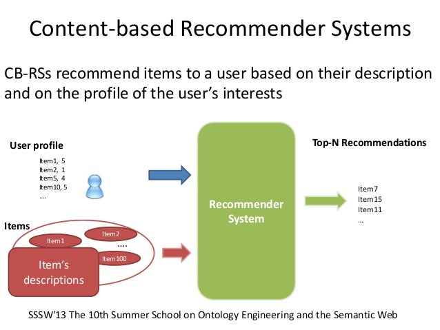
Content Based Recommendation

mov

In [279]:
from sklearn.feature_extraction.text import TfidfVectorizer
mov

In [280]:
tf = TfidfVectorizer()
tfidf_matrix = tf.fit_transform(df1['Genre'])
In [281]:
print(tfidf_matrix.todense().shape)
(1000, 21)
In [295]:
a = pd.DataFrame(tfidf_matrix.todense())
a
Out[295]:
0 1 2 3 4 5 6 7 8 9 ... 11 12 13 14 15 16 17 18 19 20
0 0.402181 0.430870 0.000000 0.000000 0.000000 0.000000 0.000000 0.000000 0.000000 0.571227 ... 0.000000 0.000000 0.000000 0.000000 0.000000 0.571227 0.000000 0.000000 0.0 0.0
1 0.000000 0.394839 0.000000 0.000000 0.000000 0.000000 0.000000 0.000000 0.000000 0.523459 ... 0.000000 0.000000 0.000000 0.544136 0.000000 0.523459 0.000000 0.000000 0.0 0.0
2 0.000000 0.000000 0.000000 0.000000 0.000000 0.000000 0.000000 0.000000 0.000000 0.000000 ... 0.764645 0.000000 0.000000 0.000000 0.000000 0.000000 0.000000 0.644452 0.0 0.0
3 0.000000 0.000000 0.658782 0.000000 0.374818 0.000000 0.000000 0.652317 0.000000 0.000000 ... 0.000000 0.000000 0.000000 0.000000 0.000000 0.000000 0.000000 0.000000 0.0 0.0
4 0.477136 0.511172 0.000000 0.000000 0.000000 0.000000 0.000000 0.000000 0.714874 0.000000 ... 0.000000 0.000000 0.000000 0.000000 0.000000 0.000000 0.000000 0.000000 0.0 0.0
5 0.477136 0.511172 0.000000 0.000000 0.000000 0.000000 0.000000 0.000000 0.714874 0.000000 ... 0.000000 0.000000 0.000000 0.000000 0.000000 0.000000 0.000000 0.000000 0.0 0.0
6 0.000000 0.000000 0.000000 0.000000 0.391659 0.000000 0.287037 0.000000 0.000000 0.000000 ... 0.000000 0.874193 0.000000 0.000000 0.000000 0.000000 0.000000 0.000000 0.0 0.0
7 0.000000 0.000000 0.000000 0.000000 1.000000 0.000000 0.000000 0.000000 0.000000 0.000000 ... 0.000000 0.000000 0.000000 0.000000 0.000000 0.000000 0.000000 0.000000 0.0 0.0
8 0.461223 0.494125 0.000000 0.736963 0.000000 0.000000 0.000000 0.000000 0.000000 0.000000 ... 0.000000 0.000000 0.000000 0.000000 0.000000 0.000000 0.000000 0.000000 0.0 0.0
9 0.000000 0.569315 0.000000 0.000000 0.000000 0.000000 0.404068 0.000000 0.000000 0.000000 ... 0.000000 0.000000 0.000000 0.000000 0.715968 0.000000 0.000000 0.000000 0.0 0.0
10 0.000000 0.415354 0.000000 0.000000 0.000000 0.000000 0.000000 0.700049 0.580872 0.000000 ... 0.000000 0.000000 0.000000 0.000000 0.000000 0.000000 0.000000 0.000000 0.0 0.0
11 0.000000 0.000000 0.000000 0.588934 0.000000 0.000000 0.280259 0.000000 0.000000 0.000000 ... 0.000000 0.000000 0.000000 0.000000 0.000000 0.000000 0.000000 0.000000 0.0 0.0
12 0.402181 0.430870 0.000000 0.000000 0.000000 0.000000 0.000000 0.000000 0.000000 0.571227 ... 0.000000 0.000000 0.000000 0.000000 0.000000 0.571227 0.000000 0.000000 0.0 0.0
13 0.000000 0.454774 0.774086 0.000000 0.440421 0.000000 0.000000 0.000000 0.000000 0.000000 ... 0.000000 0.000000 0.000000 0.000000 0.000000 0.000000 0.000000 0.000000 0.0 0.0
14 0.613760 0.000000 0.000000 0.000000 0.636790 0.000000 0.466687 0.000000 0.000000 0.000000 ... 0.000000 0.000000 0.000000 0.000000 0.000000 0.000000 0.000000 0.000000 0.0 0.0
15 0.000000 0.454774 0.774086 0.000000 0.440421 0.000000 0.000000 0.000000 0.000000 0.000000 ... 0.000000 0.000000 0.000000 0.000000 0.000000 0.000000 0.000000 0.000000 0.0 0.0
16 0.000000 0.000000 0.000000 0.588934 0.000000 0.000000 0.280259 0.000000 0.000000 0.000000 ... 0.000000 0.000000 0.000000 0.000000 0.000000 0.000000 0.000000 0.000000 0.0 0.0
17 0.640103 0.000000 0.000000 0.000000 0.000000 0.000000 0.000000 0.000000 0.000000 0.000000 ... 0.000000 0.000000 0.000000 0.000000 0.000000 0.000000 0.000000 0.768289 0.0 0.0
18 0.000000 0.000000 0.000000 0.902971 0.000000 0.000000 0.429701 0.000000 0.000000 0.000000 ... 0.000000 0.000000 0.000000 0.000000 0.000000 0.000000 0.000000 0.000000 0.0 0.0
19 0.000000 0.000000 0.000000 0.000000 0.000000 0.000000 0.291748 0.000000 0.000000 0.544964 ... 0.000000 0.000000 0.000000 0.566490 0.000000 0.544964 0.000000 0.000000 0.0 0.0
20 0.000000 0.602049 0.000000 0.000000 0.000000 0.000000 0.427301 0.000000 0.000000 0.000000 ... 0.000000 0.000000 0.000000 0.000000 0.000000 0.000000 0.000000 0.674500 0.0 0.0
21 0.000000 0.000000 0.000000 0.000000 0.000000 0.000000 1.000000 0.000000 0.000000 0.000000 ... 0.000000 0.000000 0.000000 0.000000 0.000000 0.000000 0.000000 0.000000 0.0 0.0
22 0.000000 0.000000 0.000000 0.000000 0.000000 0.632779 0.364708 0.000000 0.000000 0.000000 ... 0.683066 0.000000 0.000000 0.000000 0.000000 0.000000 0.000000 0.000000 0.0 0.0
23 0.000000 0.454774 0.774086 0.000000 0.440421 0.000000 0.000000 0.000000 0.000000 0.000000 ... 0.000000 0.000000 0.000000 0.000000 0.000000 0.000000 0.000000 0.000000 0.0 0.0
24 0.402181 0.430870 0.000000 0.000000 0.000000 0.000000 0.000000 0.000000 0.000000 0.571227 ... 0.000000 0.000000 0.000000 0.000000 0.000000 0.571227 0.000000 0.000000 0.0 0.0
25 0.000000 0.000000 0.000000 0.000000 1.000000 0.000000 0.000000 0.000000 0.000000 0.000000 ... 0.000000 0.000000 0.000000 0.000000 0.000000 0.000000 0.000000 0.000000 0.0 0.0
26 0.605680 0.648886 0.000000 0.000000 0.000000 0.000000 0.460543 0.000000 0.000000 0.000000 ... 0.000000 0.000000 0.000000 0.000000 0.000000 0.000000 0.000000 0.000000 0.0 0.0
27 0.000000 0.000000 0.000000 0.000000 0.000000 0.000000 0.000000 0.000000 0.000000 0.000000 ... 0.764645 0.000000 0.000000 0.000000 0.000000 0.000000 0.000000 0.644452 0.0 0.0
28 0.000000 0.000000 0.000000 0.000000 1.000000 0.000000 0.000000 0.000000 0.000000 0.000000 ... 0.000000 0.000000 0.000000 0.000000 0.000000 0.000000 0.000000 0.000000 0.0 0.0
29 0.605680 0.648886 0.000000 0.000000 0.000000 0.000000 0.460543 0.000000 0.000000 0.000000 ... 0.000000 0.000000 0.000000 0.000000 0.000000 0.000000 0.000000 0.000000 0.0 0.0
... ... ... ... ... ... ... ... ... ... ... ... ... ... ... ... ... ... ... ... ... ...
970 0.000000 0.000000 0.000000 0.000000 0.000000 0.000000 0.000000 0.000000 0.000000 0.000000 ... 0.764645 0.000000 0.000000 0.000000 0.000000 0.000000 0.000000 0.644452 0.0 0.0
971 0.000000 0.000000 0.000000 0.000000 0.000000 0.000000 0.371085 0.000000 0.000000 0.000000 ... 0.000000 0.000000 0.000000 0.720541 0.000000 0.000000 0.000000 0.585762 0.0 0.0
972 0.000000 0.000000 0.000000 0.000000 0.337613 0.000000 0.247428 0.000000 0.000000 0.000000 ... 0.000000 0.000000 0.908183 0.000000 0.000000 0.000000 0.000000 0.000000 0.0 0.0
973 0.000000 0.000000 0.000000 0.000000 0.000000 0.000000 0.000000 0.000000 0.000000 0.000000 ... 0.694240 0.000000 0.000000 0.719744 0.000000 0.000000 0.000000 0.000000 0.0 0.0
974 0.000000 0.000000 0.000000 0.555907 0.000000 0.000000 0.264542 0.000000 0.000000 0.000000 ... 0.000000 0.000000 0.000000 0.000000 0.000000 0.000000 0.788026 0.000000 0.0 0.0
975 0.000000 0.000000 0.000000 0.000000 0.418298 0.000000 0.000000 0.727988 0.000000 0.000000 ... 0.000000 0.000000 0.000000 0.000000 0.543194 0.000000 0.000000 0.000000 0.0 0.0
976 0.000000 0.000000 0.000000 0.000000 0.000000 0.000000 0.371085 0.000000 0.000000 0.000000 ... 0.000000 0.000000 0.000000 0.720541 0.000000 0.000000 0.000000 0.585762 0.0 0.0
977 0.000000 0.000000 0.000000 0.000000 1.000000 0.000000 0.000000 0.000000 0.000000 0.000000 ... 0.000000 0.000000 0.000000 0.000000 0.000000 0.000000 0.000000 0.000000 0.0 0.0
978 0.000000 0.000000 0.000000 0.000000 0.000000 0.000000 1.000000 0.000000 0.000000 0.000000 ... 0.000000 0.000000 0.000000 0.000000 0.000000 0.000000 0.000000 0.000000 0.0 0.0
979 0.000000 0.000000 0.000000 0.000000 0.000000 0.000000 0.535157 0.000000 0.000000 0.000000 ... 0.000000 0.000000 0.000000 0.000000 0.000000 0.000000 0.000000 0.844752 0.0 0.0
980 0.000000 0.000000 0.000000 0.632014 0.000000 0.000000 0.300760 0.714214 0.000000 0.000000 ... 0.000000 0.000000 0.000000 0.000000 0.000000 0.000000 0.000000 0.000000 0.0 0.0
981 0.000000 0.000000 0.000000 0.000000 0.467988 0.000000 0.342976 0.814466 0.000000 0.000000 ... 0.000000 0.000000 0.000000 0.000000 0.000000 0.000000 0.000000 0.000000 0.0 0.0
982 0.000000 0.000000 0.000000 0.000000 0.000000 0.000000 0.233411 0.000000 0.459920 0.000000 ... 0.000000 0.000000 0.856734 0.000000 0.000000 0.000000 0.000000 0.000000 0.0 0.0
983 0.000000 0.000000 0.000000 0.000000 1.000000 0.000000 0.000000 0.000000 0.000000 0.000000 ... 0.000000 0.000000 0.000000 0.000000 0.000000 0.000000 0.000000 0.000000 0.0 0.0
984 0.000000 0.510266 0.000000 0.000000 0.000000 0.000000 0.000000 0.860017 0.000000 0.000000 ... 0.000000 0.000000 0.000000 0.000000 0.000000 0.000000 0.000000 0.000000 0.0 0.0
985 0.000000 0.506781 0.000000 0.000000 0.490786 0.000000 0.000000 0.000000 0.708733 0.000000 ... 0.000000 0.000000 0.000000 0.000000 0.000000 0.000000 0.000000 0.000000 0.0 0.0
986 0.000000 0.000000 0.000000 0.000000 0.000000 0.000000 0.000000 0.000000 0.000000 0.000000 ... 0.764645 0.000000 0.000000 0.000000 0.000000 0.000000 0.000000 0.644452 0.0 0.0
987 0.000000 0.000000 0.000000 0.000000 0.000000 0.000000 0.491495 0.000000 0.000000 0.000000 ... 0.000000 0.000000 0.000000 0.000000 0.870880 0.000000 0.000000 0.000000 0.0 0.0
988 0.000000 0.000000 0.000000 0.000000 0.000000 0.000000 0.000000 0.000000 0.000000 0.000000 ... 1.000000 0.000000 0.000000 0.000000 0.000000 0.000000 0.000000 0.000000 0.0 0.0
989 0.000000 0.000000 0.000000 0.588934 0.000000 0.000000 0.280259 0.000000 0.000000 0.000000 ... 0.000000 0.000000 0.000000 0.000000 0.000000 0.000000 0.000000 0.000000 0.0 0.0
990 0.477136 0.511172 0.000000 0.000000 0.000000 0.000000 0.000000 0.000000 0.714874 0.000000 ... 0.000000 0.000000 0.000000 0.000000 0.000000 0.000000 0.000000 0.000000 0.0 0.0
991 0.000000 0.000000 0.000000 0.000000 0.000000 0.000000 0.250669 0.595264 0.000000 0.000000 ... 0.000000 0.763431 0.000000 0.000000 0.000000 0.000000 0.000000 0.000000 0.0 0.0
992 0.000000 0.000000 0.000000 0.000000 0.556983 0.000000 0.408199 0.000000 0.000000 0.000000 ... 0.000000 0.000000 0.000000 0.000000 0.723287 0.000000 0.000000 0.000000 0.0 0.0
993 0.489359 0.524267 0.000000 0.000000 0.000000 0.000000 0.000000 0.000000 0.000000 0.000000 ... 0.696902 0.000000 0.000000 0.000000 0.000000 0.000000 0.000000 0.000000 0.0 0.0
994 0.000000 0.000000 0.000000 0.000000 1.000000 0.000000 0.000000 0.000000 0.000000 0.000000 ... 0.000000 0.000000 0.000000 0.000000 0.000000 0.000000 0.000000 0.000000 0.0 0.0
995 0.000000 0.000000 0.000000 0.000000 0.000000 0.622014 0.358504 0.000000 0.000000 0.000000 ... 0.000000 0.000000 0.000000 0.696113 0.000000 0.000000 0.000000 0.000000 0.0 0.0
996 0.000000 0.000000 0.000000 0.000000 0.000000 0.000000 0.000000 0.000000 0.000000 0.000000 ... 1.000000 0.000000 0.000000 0.000000 0.000000 0.000000 0.000000 0.000000 0.0 0.0
997 0.000000 0.000000 0.000000 0.000000 0.000000 0.000000 0.273025 0.000000 0.000000 0.000000 ... 0.000000 0.831517 0.000000 0.000000 0.483773 0.000000 0.000000 0.000000 0.0 0.0
998 0.000000 0.718352 0.000000 0.000000 0.695680 0.000000 0.000000 0.000000 0.000000 0.000000 ... 0.000000 0.000000 0.000000 0.000000 0.000000 0.000000 0.000000 0.000000 0.0 0.0
999 0.000000 0.000000 0.000000 0.000000 0.404418 0.000000 0.000000 0.703831 0.584010 0.000000 ... 0.000000 0.000000 0.000000 0.000000 0.000000 0.000000 0.000000 0.000000 0.0 0.0

1000 rows × 21 columns

In [296]:
from sklearn.metrics.pairwise import cosine_similarity

mov

Building a matrix with cosine similarity scores

In [297]:
cosine_sim = cosine_similarity(tfidf_matrix, tfidf_matrix)
print(cosine_sim)
[[1.         0.76815261 0.         ... 0.         0.30951647 0.        ]
 [0.76815261 1.         0.         ... 0.         0.28363342 0.        ]
 [0.         0.         1.         ... 0.         0.         0.        ]
 ...
 [0.         0.         0.         ... 1.         0.         0.        ]
 [0.30951647 0.28363342 0.         ... 0.         1.         0.28134523]
 [0.         0.         0.         ... 0.         0.28134523 1.        ]]

Build a 1-dimensional array with movie titles

In [298]:
titles = df1['Title']
indices = pd.Series(df.index, index=df1['Title'])
print(indices.head(10))
Title
Guardians of the Galaxy    0
Prometheus                 1
Split                      2
Sing                       3
Suicide Squad              4
The Great Wall             5
La La Land                 6
Mindhorn                   7
The Lost City of Z         8
Passengers                 9
dtype: int64

Function that get movie recommendations based on the cosine similarity score of movie genres

In [299]:
def genre_recommendations(title):
    sim_scores = list(enumerate(cosine_sim[indices[title]]))
    
    # Sorting the recommendation list according to cosine similarity
    sim_scores = sorted(sim_scores, key=lambda x: x[1], reverse=True)
    
    # Printing the top 30 recommendations in desencding order of similarity score
    sim_scores = sim_scores[1:30]
    
    # Indexing with Integer Location and returning the values
    movie_indices = [i[0] for i in sim_scores]
    return titles.iloc[movie_indices]

Recommendation Based on the cosine simialrity and sorted according to similarity scores

In [300]:
genre_recommendations('Guardians of the Galaxy')
Out[300]:
12                               Rogue One
24            Independence Day: Resurgence
32                       X-Men: Apocalypse
35              Captain America: Civil War
48                        Star Trek Beyond
60      Batman v Superman: Dawn of Justice
67                      Mad Max: Fury Road
80                               Inception
85                          Jurassic World
94                 Avengers: Age of Ultron
126        Transformers: Age of Extinction
140                              Star Trek
156                            Pacific Rim
162             X-Men: Days of Future Past
195     Captain America: The First Avenger
200                       Edge of Tomorrow
203                               Iron Man
205                         X: First Class
212                           Transformers
216    Captain America: The Winter Soldier
220                         Hardcore Henry
227                              Predators
243                     Terminator Genisys
253               The Amazing Spider-Man 2
256                             Battleship
268               X-Men Origins: Wolverine
279                         Iron Man Three
287                      Jupiter Ascending
316                           The 5th Wave
Name: Title, dtype: object

Summary

From the above given dataset we built a content based Recommendation system or Personalized recommendation system.First we had to clean the datset as there were some missing values then we had to drop the columns which didn't seem necessary for out Analysis. After that we did some Exploratory Data Analysis on the movie dataset and found some trends and observations from the plots.

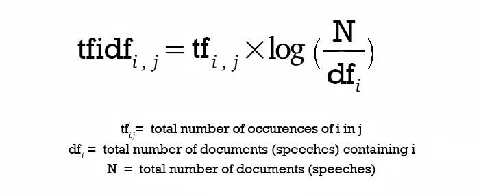
Then we used the concept of TF-IDF vector to convert our texts into a matrix form and find the cosine similarity so that we can predict the similar movies present in the dataset. At last we were sucessfull in building a very small version of a personalized recommendation system.