Problem Statement
Dataset containing several tweets with positive and negative sentiment associated with it
Cyber bullying and hate speech has been a menace for quite a long time,So our objective for this task is to detect speeches tweets associated with negative sentiments.From this dataset we classify a tweet as hate speech if it has racist or sexist tweets associated with it.
So our task here is to classify racist and sexist tweets from other tweets and filter them out.

Dataset Description
- The data is in csv format.In computing, a comma-separated values (CSV) file stores tabular data (numbers and text) in plain text.Each line of the file is a data record. Each record consists of one or more fields, separated by commas.
- Formally, given a training sample of tweets and labels, where label ‘1’ denotes the tweet is racist/sexist and label ‘0’ denotes the tweet is not racist/sexist,our objective is to predict the labels on the given test dataset.
Attribute Information
- id : The id associated with the tweets in the given dataset
- tweets : The tweets collected from various sources and having either postive or negative sentiments associated with it
- label : A tweet with label '0' is of positive sentiment while a tweet with label '1' is of negative sentiment
Importing the necessary packages
import re
import pandas as pd
import numpy as np
import matplotlib.pyplot as plt
import seaborn as sns
import string
import nltk
import warnings
warnings.filterwarnings("ignore", category=DeprecationWarning)

%matplotlib inline
Train dataset used for our analysis
train = pd.read_csv('https://raw.githubusercontent.com/dD2405/Twitter_Sentiment_Analysis/master/train.csv')
We make a copy of training data so that even if we have to make any changes in this dataset we would not lose the original dataset.
train_original=train.copy()
Here we see that there are a total of 31692 tweets in the training dataset
train.shape
train_original
Test dataset used for our analysis
test = pd.read_csv('https://raw.githubusercontent.com/dD2405/Twitter_Sentiment_Analysis/master/test.csv')
We make a copy of test data so that even if we have to make any changes in this dataset we would not lose the original dataset.
test_original=test.copy()
Here we see that there are a total of 17197 tweets in the test dataset
test.shape
test_original
We combine Train and Test datasets for pre-processing stage
combine = train.append(test,ignore_index=True,sort=True)
combine.head()
combine.tail()
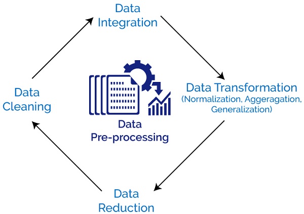
Data Pre-Processing

Removing Twitter Handles (@user)
Given below is a user-defined function to remove unwanted text patterns from the tweets. It takes two arguments, one is the original string of text and the other is the pattern of text that we want to remove from the string. The function returns the same input string but without the given pattern. We will use this function to remove the pattern ‘@user’ from all the tweets in our data.
def remove_pattern(text,pattern):

    # re.findall() finds the pattern i.e @user and puts it in a list for further task
    r = re.findall(pattern,text)

    # re.sub() removes @user from the sentences in the dataset
    for i in r:
        text = re.sub(i,"",text)

    return text
combine['Tidy_Tweets'] = np.vectorize(remove_pattern)(combine['tweet'], "@[\w]*")

combine.head()
Removing Punctuations, Numbers, and Special Characters
Punctuations, numbers and special characters do not help much. It is better to remove them from the text just as we removed the twitter handles. Here we will replace everything except characters and hashtags with spaces.
combine['Tidy_Tweets'] = combine['Tidy_Tweets'].str.replace("[^a-zA-Z#]", " ")
combine.head(10)
Removing Short Words
We have to be a little careful here in selecting the length of the words which we want to remove. So, I have decided to remove all the words having length 3 or less. For example, terms like “hmm”, “oh” are of very little use. It is better to get rid of them.
combine['Tidy_Tweets'] = combine['Tidy_Tweets'].apply(lambda x: ' '.join([w for w in x.split() if len(w)>3]))

combine.head(10)
Tokenization
Now we will tokenize all the cleaned tweets in our dataset. Tokens are individual terms or words, and tokenization is the process of splitting a string of text into tokens.
tokenized_tweet = combine['Tidy_Tweets'].apply(lambda x: x.split())
tokenized_tweet.head()
Stemming
Stemming is a rule-based process of stripping the suffixes (“ing”, “ly”, “es”, “s” etc) from a word. For example, For example – “play”, “player”, “played”, “plays” and “playing” are the different variations of the word – “play”
from nltk import PorterStemmer

ps = PorterStemmer()

tokenized_tweet = tokenized_tweet.apply(lambda x: [ps.stem(i) for i in x])

tokenized_tweet.head()
Now let’s stitch these tokens back together.
for i in range(len(tokenized_tweet)):
    tokenized_tweet[i] = ' '.join(tokenized_tweet[i])

combine['Tidy_Tweets'] = tokenized_tweet
combine.head()
Visualization from Tweets

WordCloud

A wordcloud is a visualization wherein the most frequent words appear in large size and the less frequent words appear in smaller sizes.
Importing Packages necessary for generating a WordCloud
from wordcloud import WordCloud,ImageColorGenerator
from PIL import Image
import urllib
import requests
Store all the words from the dataset which are non-racist/sexist
all_words_positive = ' '.join(text for text in combine['Tidy_Tweets'][combine['label']==0])
We can see most of the words are positive or neutral. With happy, smile, and love being the most frequent ones. Hence, most of the frequent words are compatible with the sentiment which is non racist/sexists tweets.
# combining the image with the dataset
Mask = np.array(Image.open(requests.get('http://clipart-library.com/image_gallery2/Twitter-PNG-Image.png', stream=True).raw))

# We use the ImageColorGenerator library from Wordcloud
# Here we take the color of the image and impose it over our wordcloud
image_colors = ImageColorGenerator(Mask)

# Now we use the WordCloud function from the wordcloud library
wc = WordCloud(background_color='black', height=1500, width=4000,mask=Mask).generate(all_words_positive)

# Size of the image generated
plt.figure(figsize=(10,20))

# Here we recolor the words from the dataset to the image's color
# recolor just recolors the default colors to the image's blue color
# interpolation is used to smooth the image generated
plt.imshow(wc.recolor(color_func=image_colors),interpolation="hamming")

plt.axis('off')
plt.show()
Store all the words from the dataset which are racist/sexist
all_words_negative = ' '.join(text for text in combine['Tidy_Tweets'][combine['label']==1])
As we can clearly see, most of the words have negative connotations. So, it seems we have a pretty good text data to work on.
# combining the image with the dataset
Mask = np.array(Image.open(requests.get('http://clipart-library.com/image_gallery2/Twitter-PNG-Image.png', stream=True).raw))

# We use the ImageColorGenerator library from Wordcloud
# Here we take the color of the image and impose it over our wordcloud
image_colors = ImageColorGenerator(Mask)

# Now we use the WordCloud function from the wordcloud library
wc = WordCloud(background_color='black', height=1500, width=4000,mask=Mask).generate(all_words_negative)

# Size of the image generated
plt.figure(figsize=(10,20))

# Here we recolor the words from the dataset to the image's color
# recolor just recolors the default colors to the image's blue color
# interpolation is used to smooth the image generated
plt.imshow(wc.recolor(color_func=image_colors),interpolation="gaussian")

plt.axis('off')
plt.show()
Understanding the impact of Hashtags on tweets sentiment

Function to extract hashtags from tweets
def Hashtags_Extract(x):
    hashtags=[]

    # Loop over the words in the tweet
    for i in x:
        ht = re.findall(r'#(\w+)',i)
        hashtags.append(ht)

    return hashtags
A nested list of all the hashtags from the positive reviews from the dataset
ht_positive = Hashtags_Extract(combine['Tidy_Tweets'][combine['label']==0])
Here we unnest the list
ht_positive_unnest = sum(ht_positive,[])
A nested list of all the hashtags from the negative reviews from the dataset
ht_negative = Hashtags_Extract(combine['Tidy_Tweets'][combine['label']==1])
Here we unnest the list
ht_negative_unnest = sum(ht_negative,[])
Plotting BarPlots

For Positive Tweets in the dataset
Counting the frequency of the words having Positive Sentiment
word_freq_positive = nltk.FreqDist(ht_positive_unnest)

word_freq_positive
Creating a dataframe for the most frequently used words in hashtags
df_positive = pd.DataFrame({'Hashtags':list(word_freq_positive.keys()),'Count':list(word_freq_positive.values())})
df_positive.head(10)
Plotting the barplot for the 10 most frequent words used for hashtags
df_positive_plot = df_positive.nlargest(20,columns='Count')
sns.barplot(data=df_positive_plot,y='Hashtags',x='Count')
sns.despine()
For Negative Tweets in the dataset
Counting the frequency of the words having Negative Sentiment
word_freq_negative = nltk.FreqDist(ht_negative_unnest)
word_freq_negative
Creating a dataframe for the most frequently used words in hashtags
df_negative = pd.DataFrame({'Hashtags':list(word_freq_negative.keys()),'Count':list(word_freq_negative.values())})
df_negative.head(10)
Plotting the barplot for the 10 most frequent words used for hashtags
df_negative_plot = df_negative.nlargest(20,columns='Count')
sns.barplot(data=df_negative_plot,y='Hashtags',x='Count')
sns.despine()
Extracting Features from cleaned Tweets
Bag-of-Words Features
Bag of Words is a method to extract features from text documents. These features can be used for training machine learning algorithms. It creates a vocabulary of all the unique words occurring in all the documents in the training set.
Consider a corpus (a collection of texts) called C of D documents {d1,d2…..dD} and N unique tokens extracted out of the corpus C. The N tokens (words) will form a list, and the size of the bag-of-words matrix M will be given by D X N. Each row in the matrix M contains the frequency of tokens in document D(i).
For example, if you have 2 documents-
D1: He is a lazy boy. She is also lazy.
D2: Smith is a lazy person.
First, it creates a vocabulary using unique words from all the documents
[‘He’ , ’She’ , ’lazy’ , 'boy’ , 'Smith’ , ’person’]
- Here, D=2, N=6
- The matrix M of size 2 X 6 will be represented as:

The above table depicts the training features containing term frequencies of each word in each document. This is called bag-of-words approach since the number of occurrence and not sequence or order of words matters in this approach.
from sklearn.feature_extraction.text import CountVectorizer

bow_vectorizer = CountVectorizer(max_df=0.90, min_df=2, max_features=1000, stop_words='english')

# bag-of-words feature matrix
bow = bow_vectorizer.fit_transform(combine['Tidy_Tweets'])

df_bow = pd.DataFrame(bow.todense())

df_bow
TF-IDF Features
Tf-idf stands for term frequency-inverse document frequency, and the tf-idf weight is a weight often used in information retrieval and text mining. This weight is a statistical measure used to evaluate how important a word is to a document in a collection or corpus. The importance increases proportionally to the number of times a word appears in the document but is offset by the frequency of the word in the corpus.
Typically, the tf-idf weight is composed by two terms: the first computes the normalized Term Frequency (TF), aka. the number of times a word appears in a document, divided by the total number of words in that document; the second term is the Inverse Document Frequency (IDF), computed as the logarithm of the number of the documents in the corpus divided by the number of documents where the specific term appears.
TF: Term Frequency, which measures how frequently a term occurs in a document. Since every document is different in length, it is possible that a term would appear much more times in long documents than shorter ones. Thus, the term frequency is often divided by the document length (aka. the total number of terms in the document) as a way of normalization: #### TF(t) = (Number of times term t appears in a document) / (Total number of terms in the document).
IDF: Inverse Document Frequency, which measures how important a term is. While computing TF, all terms are considered equally important. However it is known that certain terms, such as "is", "of", and "that", may appear a lot of times but have little importance. Thus we need to weigh down the frequent terms while scale up the rare ones, by computing the following: #### IDF(t) = log_e(Total number of documents / Number of documents with term t in it).
Example:
Consider a document containing 100 words wherein the word cat appears 3 times. The term frequency (i.e., tf) for cat is then (3 / 100) = 0.03. Now, assume we have 10 million documents and the word cat appears in one thousand of these. Then, the inverse document frequency (i.e., idf) is calculated as log(10,000,000 / 1,000) = 4. Thus, the Tf-idf weight is the product of these quantities: 0.03 * 4 = 0.12.

from sklearn.feature_extraction.text import TfidfVectorizer

tfidf=TfidfVectorizer(max_df=0.90, min_df=2,max_features=1000,stop_words='english')

tfidf_matrix=tfidf.fit_transform(combine['Tidy_Tweets'])

df_tfidf = pd.DataFrame(tfidf_matrix.todense())

df_tfidf
Applying Machine Learning Models
 )
)
Using the features from Bag-of-Words Model for training set
train_bow = bow[:31962]

train_bow.todense()
Using features from TF-IDF for training set
train_tfidf_matrix = tfidf_matrix[:31962]

train_tfidf_matrix.todense()
Splitting the data into training and validation set
from sklearn.model_selection import train_test_split
Bag-of-Words Features
x_train_bow,x_valid_bow,y_train_bow,y_valid_bow = train_test_split(train_bow,train['label'],test_size=0.3,random_state=2)
Using TF-IDF features
x_train_tfidf,x_valid_tfidf,y_train_tfidf,y_valid_tfidf = train_test_split(train_tfidf_matrix,train['label'],test_size=0.3,random_state=17)
Logistic Regression
from sklearn.linear_model import LogisticRegression
Log_Reg = LogisticRegression(random_state=0,solver='lbfgs')
Using Bag-of-Words Features
# Fitting the Logistic Regression Model

Log_Reg.fit(x_train_bow,y_train_bow)
# The first part of the list is predicting probabilities for label:0
# and the second part of the list is predicting probabilities for label:1
prediction_bow = Log_Reg.predict_proba(x_valid_bow)

prediction_bow
Calculating the F1 score
from sklearn.metrics import f1_score
# if prediction is greater than or equal to 0.3 than 1 else 0
# Where 0 is for positive sentiment tweets and 1 for negative sentiment tweets
prediction_int = prediction_bow[:,1]>=0.3

prediction_int = prediction_int.astype(np.int)
prediction_int

# calculating f1 score
log_bow = f1_score(y_valid_bow, prediction_int)

log_bow
Using TF-IDF Features
Log_Reg.fit(x_train_tfidf,y_train_tfidf)
prediction_tfidf = Log_Reg.predict_proba(x_valid_tfidf)

prediction_tfidf
Calculating the F1 score
prediction_int = prediction_tfidf[:,1]>=0.3

prediction_int = prediction_int.astype(np.int)
prediction_int

# calculating f1 score
log_tfidf = f1_score(y_valid_tfidf, prediction_int)

log_tfidf
XGBoost
from xgboost import XGBClassifier
Using Bag-of-Words Features
model_bow = XGBClassifier(random_state=22,learning_rate=0.9)
model_bow.fit(x_train_bow, y_train_bow)
# The first part of the list is predicting probabilities for label:0
# and the second part of the list is predicting probabilities for label:1
xgb=model_bow.predict_proba(x_valid_bow)

xgb
Calculating the F1 score
# if prediction is greater than or equal to 0.3 than 1 else 0
# Where 0 is for positive sentiment tweets and 1 for negative sentiment tweets
xgb=xgb[:,1]>=0.3

# converting the results to integer type
xgb_int=xgb.astype(np.int)

# calculating f1 score
xgb_bow=f1_score(y_valid_bow,xgb_int)

xgb_bow
Using TF-IDF Features
model_tfidf=XGBClassifier(random_state=29,learning_rate=0.7)
model_tfidf.fit(x_train_tfidf, y_train_tfidf)
# The first part of the list is predicting probabilities for label:0
# and the second part of the list is predicting probabilities for label:1
xgb_tfidf=model_tfidf.predict_proba(x_valid_tfidf)

xgb_tfidf
Calculating the F1 score
# if prediction is greater than or equal to 0.3 than 1 else 0
# Where 0 is for positive sentiment tweets and 1 for negative sentiment tweets
xgb_tfidf=xgb_tfidf[:,1]>=0.3

# converting the results to integer type
xgb_int_tfidf=xgb_tfidf.astype(np.int)

# calculating f1 score
score=f1_score(y_valid_tfidf,xgb_int_tfidf)

score
Decision Tree
from sklearn.tree import DecisionTreeClassifier
dct = DecisionTreeClassifier(criterion='entropy', random_state=1)
Using Bag-of-Words Features
dct.fit(x_train_bow,y_train_bow)
dct_bow = dct.predict_proba(x_valid_bow)

dct_bow
# if prediction is greater than or equal to 0.3 than 1 else 0
# Where 0 is for positive sentiment tweets and 1 for negative sentiment tweets
dct_bow=dct_bow[:,1]>=0.3

# converting the results to integer type
dct_int_bow=dct_bow.astype(np.int)

# calculating f1 score
dct_score_bow=f1_score(y_valid_bow,dct_int_bow)

dct_score_bow
Using TF-IDF Features
dct.fit(x_train_tfidf,y_train_tfidf)
dct_tfidf = dct.predict_proba(x_valid_tfidf)

dct_tfidf
Calculating F1 Score
# if prediction is greater than or equal to 0.3 than 1 else 0
# Where 0 is for positive sentiment tweets and 1 for negative sentiment tweets
dct_tfidf=dct_tfidf[:,1]>=0.3

# converting the results to integer type
dct_int_tfidf=dct_tfidf.astype(np.int)

# calculating f1 score
dct_score_tfidf=f1_score(y_valid_tfidf,dct_int_tfidf)

dct_score_tfidf
Model Comparison
Algo=['LogisticRegression(Bag-of-Words)','XGBoost(Bag-of-Words)','DecisionTree(Bag-of-Words)','LogisticRegression(TF-IDF)','XGBoost(TF-IDF)','DecisionTree(TF-IDF)']
score = [log_bow,xgb_bow,dct_score_bow,log_tfidf,score,dct_score_tfidf]

compare=pd.DataFrame({'Model':Algo,'F1_Score':score},index=[i for i in range(1,7)])
compare.T
plt.figure(figsize=(18,5))

sns.pointplot(x='Model',y='F1_Score',data=compare)

plt.title('Model Vs Score')
plt.xlabel('MODEL')
plt.ylabel('SCORE')

plt.show()
test_tfidf = tfidf_matrix[31962:]
test_pred = Log_Reg.predict_proba(test_tfidf)

test_pred_int = test_pred[:,1] >= 0.3

test_pred_int = test_pred_int.astype(np.int)

test['label'] = test_pred_int

submission = test[['id','label']]

submission.to_csv('result.csv', index=False)
Test dataset after prediction
res = pd.read_csv('result.csv')
res
Summary
- From the given dataset we were able to predict on which class i.e Positive or Negative does the given tweet fall into.The following data was collected from Analytics Vidhya's site.
Pre-processing
- Removing Twitter Handles(@user)
- Removing puntuation,numbers,special characters
- Removing short words i.e. words with length<3
- Tokenization
- Stemming
Data Visualisation
- Wordclouds
- Barplots
Word Embeddings used to convert words to features for our Machine Learning Model
- Bag-of-Words
- TF-IDF
Machine Learning Models used
- Logistic Regression
- XGBoost
- Decision Trees
Evaluation Metrics
- F1 score
sns.countplot(train_original['label'])
sns.despine()
Why use F1-Score instead of Accuracy ?
- From the above countplot generated above we see how imbalanced our dataset is.We can see that the values with label:0 i.e. positive sentiments are quite high in number as compared to the values with labels:1 i.e. negative sentiments.
- So when we keep accuracy as our evaluation metric there may be cases where we may encounter high number of false positives.
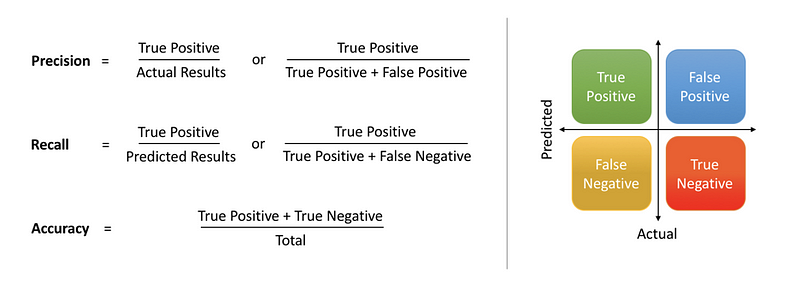
Precison & Recall :-
- Precision means the percentage of your results which are relevant.
Recall refers to the percentage of total relevant results correctly classified by your algorithm

We always face a trade-off situation between Precison and Recall i.e. High Precison gives low recall and vice versa.
- In most problems, you could either give a higher priority to maximizing precision, or recall, depending upon the problem you are trying to solve. But in general, there is a simpler metric which takes into account both precision and recall, and therefore, you can aim to maximize this number to make your model better. This metric is known as F1-score, which is simply the harmonic mean of precision and recall.

- So this metric seems much more easier and convenient to work with, as you only have to maximize one score, rather than balancing two separate scores.