.
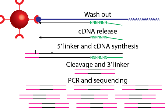
*** Presenter notes
cDNAs are released from the RNA and a 5' linker (that includes a barcode sequence and EcoP15I sequence) is ligated. Second-strand cDNA synthesis takes place and digestion with EcoP15I takes place. A 3′ linker that contains the 3′ Illumina primer sequence is ligated at the 3′ end. Amplification takes place and the tags are sequenced.
---
## Why do we perform CAGE?
> * Quantify the expression of transcripts
> * Study promoter structure and usage
> * Discover new promoters
> * Discover regulatory elements
> * For CAGE versus RNA-Seq see
*** Presenter notes
Piero and Erik showed various CAGE case studies.
---
## A typical CAGE analysis pipeline
> * The output of CAGE is a set of short nucleotide sequences and their counts.
> * Typical steps in a CAGE analysis pipeline include:
> * Tag extraction
> * Quality control steps
> * Mapping tags to a reference genome
> * Tag clustering
> * Tag cluster annotation
> * Data analysis (e.g. differential expression analysis, co-expression networks, etc.)
---
## ENCODE CAGE data
Download these BAM files into some directory:
```
path=http://hgdownload.cse.ucsc.edu/goldenPath/hg19/encodeDCC/wgEncodeRikenCage
curl -O $path/wgEncodeRikenCageHelas3CellPapRawDataRep1.fastq.gz
curl -O $path/wgEncodeRikenCageHelas3CellPapAlnRep1.bam
curl -O $path/wgEncodeRikenCageHelas3CellPapAlnRep2.bam
curl -O $path/wgEncodeRikenCageHelas3CytosolPapAlnRep1.bam
curl -O $path/wgEncodeRikenCageHelas3CytosolPapAlnRep2.bam
curl -O $path/wgEncodeRikenCageHelas3NucleusPapAlnRep1.bam
curl -O $path/wgEncodeRikenCageHelas3NucleusPapAlnRep2.bam
```
---
## Raw sequencing data
A [fastq](http://en.wikipedia.org/wiki/FASTQ_format) file contains all the reads from the sequencer.
```
gunzip -c wgEncodeRikenCageHelas3CellPapRawDataRep1.fastq.gz | head -4
@HWUSI-EAS566_0007:5:1:965:4705#0/1
NAGCAGCAGGGGAGAGTGTCATGGAGGCCTACGAGC
+HWUSI-EAS566_0007:5:1:965:4705#0/1
BYZZY\\[\[^^IXMVUUUX\]\\X[ZZ\]``^__^
```
For each read, there are four lines of information.
1. The first line is the read name and contains information on the read
2. The second line is the raw sequence of the CAGE tag
3. The third line can be used to store optional notes
4. The fourth line denotes the quality of each base call, i.e. how sure the machine is that an A is an A.
---
## Tag extraction
```
gunzip -c wgEncodeRikenCageHelas3CellPapRawDataRep1.fastq.gz | head -4
@HWUSI-EAS566_0007:5:1:965:4705#0/1
NAGCAGCAGGGGAGAGTGTCATGGAGGCCTACGAGC
+HWUSI-EAS566_0007:5:1:965:4705#0/1
BYZZY\\[\[^^IXMVUUUX\]\\X[ZZ\]``^__^
gunzip -c wgEncodeRikenCageHelas3CellPapRawDataRep1.fastq.gz | perl -nle 'if (($. - 2) % 4 == 0){ print substr($_,0,3)}' | sort | uniq -c | sort -k1,1rn | head -4
25596580 TAG
300377 TAT
158391 TCG
142412 CAG
```
The barcode for this library was TAG. The contains tools for tag extraction. See also , which uses Hidden Markov Models for tag extraction (and performs quality control steps).
*** Presenter notes
Since we know the barcode sequence, we can identify sequencing errors.
---
## Quality control
```
gunzip -c wgEncodeRikenCageHelas3CellPapRawDataRep1.fastq.gz | head -4
@HWUSI-EAS566_0007:5:1:965:4705#0/1
NAGCAGCAGGGGAGAGTGTCATGGAGGCCTACGAGC
+HWUSI-EAS566_0007:5:1:965:4705#0/1
BYZZY\\[\[^^IXMVUUUX\]\\X[ZZ\]``^__^
```
We would remove this read because it contains an ambiguous base call, especially since it's in the barcode. The quality scores range from 3 to 40:
3------------------------------------40

BCDEFGHIJKLMNOPQRSTUVWXYZ[\]^_`abcdefgh
Various different criteria to remove reads, e.g. remove reads with 10 base calls that have a quality less than 10, etc. The tool can be used to calculate and visualise read qualities.
---
## A note about quality scores
```{r, out.width='300px'}
p <- function(q){ return(10^{-q/10}) }
p(10)
plot(3:37, 1-p(3:37), xaxt='n', type='l', xlab='Quality score', ylab='Probability correct')
axis(1, 0:40); abline(h=0.9, v=10)
```
*** Presenter notes
If a base has a quality of 10, there's a 10% probability that a read is incorrect.
---
## Mapping
> * High-throughput sequencing results in millions to billions of reads
> * A computational strategy known as "indexing" speeds up mapping algorithms.
> * It works like a book index; an index of a large DNA sequence allows one to rapidly find shorter sequences embedded within it. See [How to map billions of short reads onto genomes](http://www.ncbi.nlm.nih.gov/pubmed/19430453).
> * The confidence of mapping is indicated by the mapping quality, which uses the same scale as the base calling qualities.
> * Pipelines may remove reads that have a low mapping quality.
> * I have a post on [mapping qualities](http://davetang.org/muse/2011/09/14/mapping-qualities/).
---
## SAM/BAM
A SAM/BAM file contains alignment information of a single read to a reference genome.
```
samtools view wgEncodeRikenCageHelas3CellPapAlnRep1.bam | head -3
HWUSI-EAS566_0009:3:16:8371:2418#0|TAG 16 chr1 16213 1 27M * 0 0 GCCATGCTCTGACAGTCTCAGTTGCAC fefffffffffffffdfefddffdddd NM:i:0 MD:Z:27 XP:Z:~~~~-----000077777,,,,9998:
HWUSI-EAS566_0007:5:11:4550:12891#0|TAG 16 chr1 16445 17 27M * 0 0 AGTTTGAAAACCACTATTTTATGAACC fefffffdffffffeffdffffeefff NM:i:0 MD:Z:27 XP:Z:~~~~~~~~~~~~~~~~~~~~~~~LO?~
HWUSI-EAS566_0007:5:63:12130:4370#0|TAG 0 chr1 16446 17 27M * 0 0 GTTTGAAAACCACTATTTTATGAACCA fffffdfffffdffffffffffefffe NM:i:0 MD:Z:27 XP:Z:~~~~~~~~~~~~~~~~~~~~~~~~~L~
```
If you are confused about the second column, have a look at .
---
## CAGE defined transcription starting sites
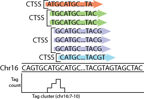 Image source: me.
---
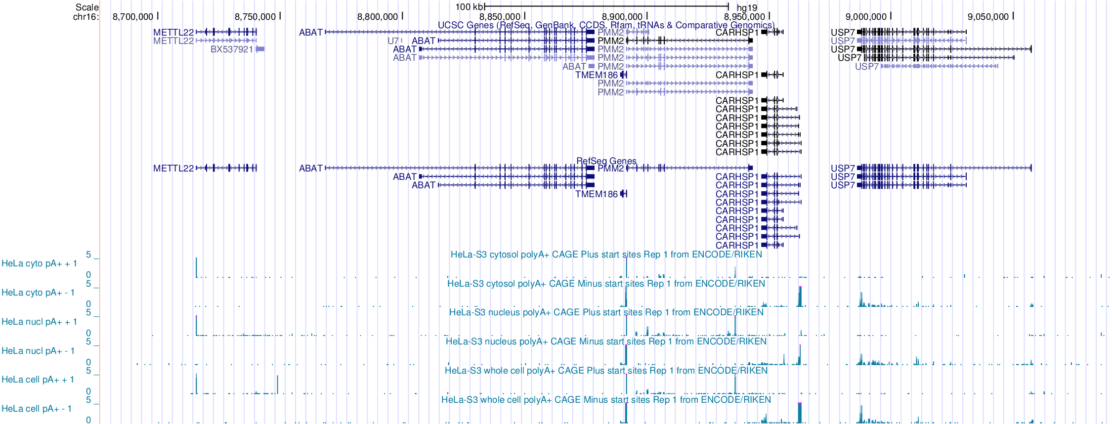
## Tag cluster annotation
Intersect/overlap tag clusters to transcript annotations
Image source: me.
---
## Tag cluster annotation
Intersect/overlap tag clusters to transcript annotations
 ---
## Intermission
* Any questions so far?
---
## A few words on R before we begin
> * I have been using R on and off for a couple of years and it takes a while to get used to.
> * Honest confession: I am not very good with R (I keep a lot of [documentation](http://davetang.org/muse/r/) to make up for this).
> * I think it is worthwhile learning because a lot of genomics analysis packages are available via the Bioconductor project.
> * By default, data loaded into R is stored into memory; the bigger your data, the more memory will be used.
---
## Bioconductor
> * From [Wikipedia](http://en.wikipedia.org/wiki/Bioconductor): Bioconductor is a free, open source and open development software project for the analysis and comprehension of genomic data generated by wet lab experiments in molecular biology.
> * Provides state of the art software to analyse various genomic datasets.
> * Has very well written guides, called vignettes, aimed at biologists.
> * To learn more take a look at these [courses](http://bioconductor.org/help/course-materials/), which are provided by the Bioconductor team.
*** Presenter notes
It's pronounced "vin 'yet".
---
## Loading data into R
Download the [data](https://dl.dropboxusercontent.com/u/15251811/pnas_expression.txt) for this [paper](http://www.ncbi.nlm.nih.gov/pubmed/19088194) (right-click on data and save as).
```{r}
getwd()
setwd("/Users/davetang/slidify_test/data/")
data <- read.table("pnas_expression.txt", header=TRUE, sep="\t", stringsAsFactors = FALSE)
head(data, 5)
```
---
## Working with data frames
```{r}
class(data)
dim(data)
data[1,]
```
---
## Removing a column
```{r}
data_subset <- data[,-9]
dim(data_subset)
head(data_subset)
```
---
## Naming the rows
```{r}
row.names(data_subset) <- data_subset[,1]
data_subset <- data_subset[,-1]
head(data_subset)
```
---
## Plotting the rowSums
```{r}
plot(density(log2(rowSums(data_subset))), xlab="Gene expression (log2)")
```
---
## Independent filtering
```{r}
dim(data_subset)
data_subset <- subset(data_subset, rowSums(data_subset)>50)
dim(data_subset)
```
See .
---
## Differential expression
```{r eval=FALSE}
source("http://bioconductor.org/biocLite.R")
biocLite("edgeR")
```
```{r, message=FALSE}
library(edgeR)
group <- c(rep("Control",4), rep("Test",3))
d <- DGEList(counts = data_subset, group=group)
#data normalisation
d <- calcNormFactors(d, method="TMM")
d <- estimateDisp(d)
et <- exactTest(d)
summary(de <- decideTestsDGE(et, p=0.05, adjust="BH"))
```
---
## Differentially expressed genes
```{r, out.width='450px'}
detags <- rownames(d)[as.logical(de)]
plotSmear(et, de.tags=detags)
abline(h = c(-2, 2), col = "blue")
```
---
## Differentially expression genes
```{r}
topTags(et, n=5)
data_subset['ENSG00000151503',]
```
---
## Saving the results
```{r}
my_genes <- data_subset[row.names(topTags(et, n=100)),]
head(my_genes, 3)
write.table(my_genes, file = "my_genes.tsv", quote = FALSE, sep = "\t")
```
---
## Intermission 2
* Any questions or comments?
---
## Correlation
See
---
## Intermission
* Any questions so far?
---
## A few words on R before we begin
> * I have been using R on and off for a couple of years and it takes a while to get used to.
> * Honest confession: I am not very good with R (I keep a lot of [documentation](http://davetang.org/muse/r/) to make up for this).
> * I think it is worthwhile learning because a lot of genomics analysis packages are available via the Bioconductor project.
> * By default, data loaded into R is stored into memory; the bigger your data, the more memory will be used.
---
## Bioconductor
> * From [Wikipedia](http://en.wikipedia.org/wiki/Bioconductor): Bioconductor is a free, open source and open development software project for the analysis and comprehension of genomic data generated by wet lab experiments in molecular biology.
> * Provides state of the art software to analyse various genomic datasets.
> * Has very well written guides, called vignettes, aimed at biologists.
> * To learn more take a look at these [courses](http://bioconductor.org/help/course-materials/), which are provided by the Bioconductor team.
*** Presenter notes
It's pronounced "vin 'yet".
---
## Loading data into R
Download the [data](https://dl.dropboxusercontent.com/u/15251811/pnas_expression.txt) for this [paper](http://www.ncbi.nlm.nih.gov/pubmed/19088194) (right-click on data and save as).
```{r}
getwd()
setwd("/Users/davetang/slidify_test/data/")
data <- read.table("pnas_expression.txt", header=TRUE, sep="\t", stringsAsFactors = FALSE)
head(data, 5)
```
---
## Working with data frames
```{r}
class(data)
dim(data)
data[1,]
```
---
## Removing a column
```{r}
data_subset <- data[,-9]
dim(data_subset)
head(data_subset)
```
---
## Naming the rows
```{r}
row.names(data_subset) <- data_subset[,1]
data_subset <- data_subset[,-1]
head(data_subset)
```
---
## Plotting the rowSums
```{r}
plot(density(log2(rowSums(data_subset))), xlab="Gene expression (log2)")
```
---
## Independent filtering
```{r}
dim(data_subset)
data_subset <- subset(data_subset, rowSums(data_subset)>50)
dim(data_subset)
```
See .
---
## Differential expression
```{r eval=FALSE}
source("http://bioconductor.org/biocLite.R")
biocLite("edgeR")
```
```{r, message=FALSE}
library(edgeR)
group <- c(rep("Control",4), rep("Test",3))
d <- DGEList(counts = data_subset, group=group)
#data normalisation
d <- calcNormFactors(d, method="TMM")
d <- estimateDisp(d)
et <- exactTest(d)
summary(de <- decideTestsDGE(et, p=0.05, adjust="BH"))
```
---
## Differentially expressed genes
```{r, out.width='450px'}
detags <- rownames(d)[as.logical(de)]
plotSmear(et, de.tags=detags)
abline(h = c(-2, 2), col = "blue")
```
---
## Differentially expression genes
```{r}
topTags(et, n=5)
data_subset['ENSG00000151503',]
```
---
## Saving the results
```{r}
my_genes <- data_subset[row.names(topTags(et, n=100)),]
head(my_genes, 3)
write.table(my_genes, file = "my_genes.tsv", quote = FALSE, sep = "\t")
```
---
## Intermission 2
* Any questions or comments?
---
## Correlation
See
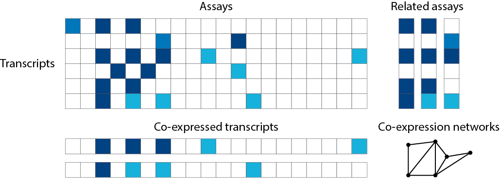 Image source: adpated from .
---
## Pairwise comparisons
```{r}
#a vs. b, a vs. c, b vs. c
choose(3,2)
choose(1000, 2)
choose(30000, 2)
```
---
## Pairwise comparisons
```{r}
plot(1000:30000, log2(choose(1000:30000, 2)), type='l', xlab="n", ylab="Pairwise comparisons (log2)")
```
---
## Hierarchical clustering
```{r, out.width='450px'}
h <- hclust(dist(t(data_subset)))
plot(h)
```
---
## Distance measure
See .
```{r}
dist(t(data_subset))
```
---
## Heatmap
See .
```{r, message=FALSE, out.width='400px'}
#install.packages("gplots")
library(gplots)
heatmap.2(as.matrix(my_genes), scale="row", trace="none")
```
---
## CAGEr
The CAGEr package available on Bioconductor provides various methods for analysing CAGE data. To install the CAGEr package:
```{r eval=FALSE}
source("http://bioconductor.org/biocLite.R")
biocLite("CAGEr")
```
To load the CAGEr package:
```{r eval=FALSE}
library(CAGEr)
```
*** Presenter notes
I decided it wasn't feasible to perform a live demo because
- CAGE data is huge
- Loading the data is slow and computationally intensive
- The vignette provides all the details
---
## What CAGEr can do
> * Quality control steps
> * CAGE normalisation
> * CAGE tag clustering
> * Analysis of promoter shape
> * Expression clustering
> * Analysis of promoter shifting
> * Importantly, we can use the CAGEr package to prepare our data for further downstream analyses.
> * For more information: .
*** Presenter notes
Michiel talked about level one and two tag clustering.
---
## Some more resources
> * I highly recommend this book called [Bioinformatics Data Skills](http://shop.oreilly.com/product/0636920030157.do). I wrote a [book review](http://davetang.org/muse/2014/04/03/bioinformatics-data-skills/) on it (on my blog of course).
> * My collection of links to various [introductory material related to bioinformatics](http://davetang.org/muse/primer/).
> * My collection of links to [resources for learning about R](http://davetang.org/muse/r/).
> * My collection of links to [courses or course material](http://davetang.org/muse/learn/) related to bioinformatics.
> * Feel free [to send me an email](mailto:me@davetang.org?subject=Hello from the MODHEP workshop!) any time.
> * Thank you for your attention!
Image source: adpated from .
---
## Pairwise comparisons
```{r}
#a vs. b, a vs. c, b vs. c
choose(3,2)
choose(1000, 2)
choose(30000, 2)
```
---
## Pairwise comparisons
```{r}
plot(1000:30000, log2(choose(1000:30000, 2)), type='l', xlab="n", ylab="Pairwise comparisons (log2)")
```
---
## Hierarchical clustering
```{r, out.width='450px'}
h <- hclust(dist(t(data_subset)))
plot(h)
```
---
## Distance measure
See .
```{r}
dist(t(data_subset))
```
---
## Heatmap
See .
```{r, message=FALSE, out.width='400px'}
#install.packages("gplots")
library(gplots)
heatmap.2(as.matrix(my_genes), scale="row", trace="none")
```
---
## CAGEr
The CAGEr package available on Bioconductor provides various methods for analysing CAGE data. To install the CAGEr package:
```{r eval=FALSE}
source("http://bioconductor.org/biocLite.R")
biocLite("CAGEr")
```
To load the CAGEr package:
```{r eval=FALSE}
library(CAGEr)
```
*** Presenter notes
I decided it wasn't feasible to perform a live demo because
- CAGE data is huge
- Loading the data is slow and computationally intensive
- The vignette provides all the details
---
## What CAGEr can do
> * Quality control steps
> * CAGE normalisation
> * CAGE tag clustering
> * Analysis of promoter shape
> * Expression clustering
> * Analysis of promoter shifting
> * Importantly, we can use the CAGEr package to prepare our data for further downstream analyses.
> * For more information: .
*** Presenter notes
Michiel talked about level one and two tag clustering.
---
## Some more resources
> * I highly recommend this book called [Bioinformatics Data Skills](http://shop.oreilly.com/product/0636920030157.do). I wrote a [book review](http://davetang.org/muse/2014/04/03/bioinformatics-data-skills/) on it (on my blog of course).
> * My collection of links to various [introductory material related to bioinformatics](http://davetang.org/muse/primer/).
> * My collection of links to [resources for learning about R](http://davetang.org/muse/r/).
> * My collection of links to [courses or course material](http://davetang.org/muse/learn/) related to bioinformatics.
> * Feel free [to send me an email](mailto:me@davetang.org?subject=Hello from the MODHEP workshop!) any time.
> * Thank you for your attention!
 Source:
 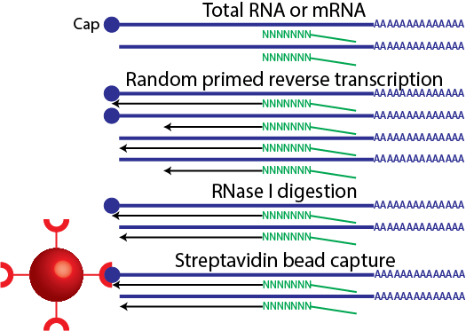 Image source: me.
*** Presenter notes
The double strand protects the RNA from RNase I digestion. However, RNAs without a Cap, are not pulled down.
---
## CAGE
Image source: me.
*** Presenter notes
The double strand protects the RNA from RNase I digestion. However, RNAs without a Cap, are not pulled down.
---
## CAGE
 For the full protocol see