{
"cells": [
{
"cell_type": "markdown",
"metadata": {},
"source": [
"# Lineare Algebra"
]
},
{
"cell_type": "markdown",
"metadata": {},
"source": [
"Die lineare Algebra beschäftigt sich mit Vektorräumen, linearen Abbildungen zwischen Vektorräumen, linearen Gleichungssystemen und Matrizen. Wichtige Anwendungen für lineare Algebra in der Computerlinguistik sind die quantitative Arbeit mit Texten und besonders Machine Learning."
]
},
{
"cell_type": "markdown",
"metadata": {},
"source": [
"Das erste Ziel ist es, Vektorräume zu definieren. Mit einem bestimmten Vektorraum führen wir dann bestimmte Rechnungen durch. \n",
"Ein Vektorraum besteht (u.a.) aus einem Körper, der (u.a.) über Gruppen definiert wird. Gruppen und Körper müssen wir also verstehen, um mit Vektorräumen arbeiten zu können.\n"
]
},
{
"cell_type": "markdown",
"metadata": {},
"source": [
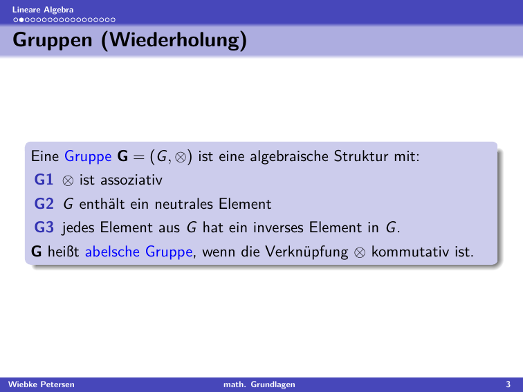
"## Gruppen\n",
"\n",
"Zuerst eine Wiederholung: Was ist eine [Gruppe](./05_Gruppen.ipynb)? Die Begriffe Assoziativität und Kommutativität, neutrales und inverses Element werden im Skript [Algebren](./05_Algebren.ipynb) erklärt. "
]
},
{
"cell_type": "markdown",
"metadata": {},
"source": [
""
]
},
{
"cell_type": "markdown",
"metadata": {},
"source": [
"## Körper"
]
},
{
"cell_type": "markdown",
"metadata": {},
"source": [
""
]
},
{
"cell_type": "markdown",
"metadata": {},
"source": [
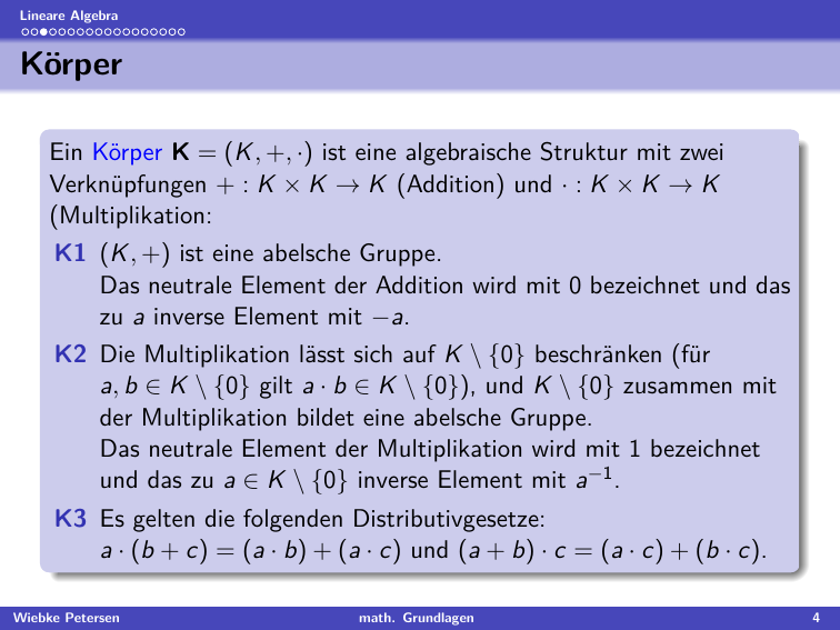
"In der Bedingung K2 wird der Körper K ohne das neutrale Element der Addition behandelt ($K\\setminus\\{0\\}$).\n",
"\n",
"Für Interessierte: Warum stehen in K3 2 Distributivgesetze? In K2 wurde die Kommmutativität von $\\cdot$ nur für $K\\setminus \\{0\\}$ explizit genannt, nicht für $K$. Deshalb gilt das Kommutativgesetz nicht zwangsläufig für alle $a,b,c\\in K$. Gilt das Kommutativgesetz für $\\cdot$ in $K$ und wir haben das gezeigt, wären die beiden Ausdrücke des Distributivgesetzes äquivalent."
]
},
{
"cell_type": "markdown",
"metadata": {},
"source": [
"## Ergänzungen"
]
},
{
"cell_type": "markdown",
"metadata": {},
"source": [
""
]
},
{
"cell_type": "markdown",
"metadata": {},
"source": [
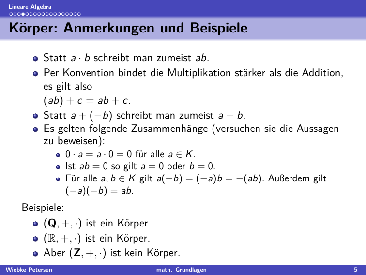
"### Wenn $ab=0$, dann $a=0$ oder $b=0$.\n",
"\n",
"Angenommen, $a,b$ sind beide $\\neq 0$. Dann gilt wegen der Kommutativität der Multiplikation: \n",
"$a\\cdot b\\cdot a^{-1}\\cdot b^{-1}=a\\cdot a^{-1}\\cdot b \\cdot b^{-1}=1\\cdot 1=1$.\n",
"Oben steht aber, dass $a\\cdot b=0$. Dann müsste ja gelten (in die Gleichung eingesetzt): \n",
"$0\\cdot a^{-1}\\cdot b^{-1}=1$\n",
"\n",
"Es gilt aber auch: $0\\cdot a=0$ für alle $a\\in K$. Daraus folgt: $0\\cdot a^{-1}\\cdot b^{-1}=0\\cdot b^{-1}=0$. Und da $0\\neq1$, kann es nicht sein, dass $a\\cdot b=0$ und $a\\neq0$ und $b\\neq 0$. Wir haben also durch Widerspruch gezeigt, dass wenn $ab=0$, dann $a=0$ oder $b=0$."
]
},
{
"cell_type": "markdown",
"metadata": {},
"source": [
"### $a(-b)=-a(b)=-(ab)$ und $(-a)(-b)=ab$\n",
"\n",
"Nehmen wir als Beispiel den Körper $(\\mathbb{R},+,\\cdot)$. \n",
"\n",
"$a=5, b=3$ und $5*(-3)=-5*3=-15$ und $(-5)*(-3)=5*3=15$\n",
"\n",
"Die Regel funktioniert genauso, wenn $a$ und/oder $b$ negativ sind. Merke: Für eine Zahl c gilt dann $-(-c)=c$."
]
},
{
"cell_type": "markdown",
"metadata": {},
"source": [
"### Warum sind die beiden ersten Beispiele Körper, das letzte Beispiel aber nicht?\n",
"\n",
"In $(\\mathbb{Z},+,\\cdot)$ ist das neutrale Element von $\\cdot$ die $1$. Z.B. ist $-7*1=-7$. Es gibt aber kein inverses Element $x\\in\\mathbb{Z}$ für $-7$, sodass $-7*x=1$."
]
},
{
"cell_type": "markdown",
"metadata": {},
"source": [
"## Vektorräume"
]
},
{
"cell_type": "markdown",
"metadata": {},
"source": [
""
]
},
{
"cell_type": "markdown",
"metadata": {},
"source": [
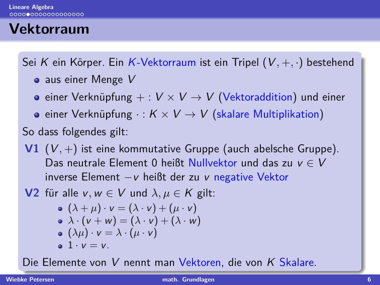
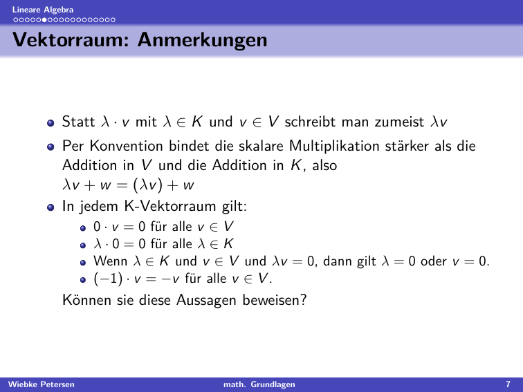
"K ist meistens $\\mathbb{R}$. Man sollte sich merken: $+$ addiert zwei Vektoren (und NICHT einen Skalar und einen Vektor), und die Multiplikation $\\cdot$, die wir hier sehen, mulitpliziert einen Skalar und einen Vektor (und NICHT zwei Vektoren). Später gibt es bei der Matrizenmultiplikation aber noch die Möglichkeit, zwei Vektoren miteinander zu multiplizieren. Achtung: Der Multiplikationsoperator $\\cdot$ ist total überladen, d.h. später arbeiten wir z.B. mit $\\cdot : K\\times V \\to V$ und auch mit der Multiplikation zweier Skalare $\\cdot : K\\times K \\to K$.\n",
"\n",
"### V2 an Beispielen\n",
"\n",
"Hier wird schon der Koordinatenraum verwendet, den einige vielleicht noch aus der Schule kennen und der weiter unten eingeführt wird.\n",
"\n",
"- $(\\lambda+\\mu)\\cdot v=(\\lambda\\cdot v)+(\\mu\\cdot v)$\n",
" $$\\lambda=6, \\mu=2, v=\\begin{pmatrix}3\\\\4\\end{pmatrix}$$\n",
" $$(6+2)*\\begin{pmatrix}3\\\\4\\end{pmatrix}=(6*\\begin{pmatrix}3\\\\4\\end{pmatrix})+(2*\\begin{pmatrix}3\\\\4\\end{pmatrix})$$\n",
" $$8*\\begin{pmatrix}3\\\\4\\end{pmatrix}=\\begin{pmatrix}6*3\\\\6*4\\end{pmatrix}+\\begin{pmatrix}2*3\\\\2*4\\end{pmatrix}$$\n",
" $$\\begin{pmatrix}8*3\\\\8*4\\end{pmatrix}=\\begin{pmatrix}18\\\\24\\end{pmatrix}+\\begin{pmatrix}6\\\\8\\end{pmatrix}$$\n",
" $$\\begin{pmatrix}24\\\\32\\end{pmatrix}=\\begin{pmatrix}24\\\\32\\end{pmatrix}$$\n",
" \n",
"- $\\lambda\\cdot(v+w)=(\\lambda\\cdot v)+\\lambda\\cdot w)$\n",
" $$\\lambda=6, v=\\begin{pmatrix}3\\\\4\\end{pmatrix}, w=\\begin{pmatrix}1\\\\1\\end{pmatrix}$$\n",
" $$6\\cdot (\\begin{pmatrix}3\\\\4\\end{pmatrix}+\\begin{pmatrix}1\\\\1\\end{pmatrix})=(6\\cdot\\begin{pmatrix}3\\\\4\\end{pmatrix})+(6\\cdot\\begin{pmatrix}1\\\\1\\end{pmatrix})$$\n",
" $$6\\cdot\\begin{pmatrix}4\\\\5\\end{pmatrix}=\\begin{pmatrix}18\\\\24\\end{pmatrix}+\\begin{pmatrix}6\\\\6\\end{pmatrix}$$\n",
" $$\\begin{pmatrix}24\\\\30\\end{pmatrix}=\\begin{pmatrix}24\\\\30\\end{pmatrix}$$\n",
" \n",
"- $(\\lambda*\\mu)\\cdot v = \\lambda \\cdot (\\mu\\cdot v)$\n",
" $$\\lambda=6, \\mu=2 v=\\begin{pmatrix}3\\\\4\\end{pmatrix}$$\n",
" $$(6*2)\\cdot\\begin{pmatrix}3\\\\4\\end{pmatrix}=6\\cdot(2\\cdot\\begin{pmatrix}3\\\\4\\end{pmatrix} $$\n",
"$$\\dots$$"
]
},
{
"cell_type": "markdown",
"metadata": {},
"source": [
""
]
},
{
"cell_type": "markdown",
"metadata": {},
"source": [
""
]
},
{
"cell_type": "markdown",
"metadata": {},
"source": [
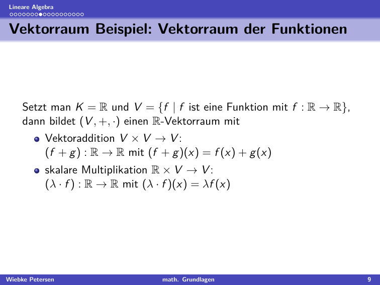
"## Vektorraum Beispiel: Vektorraum der Funktionen\n",
"\n",
"In der Vorlesung wurde noch ein weiterer Vektorraum vorgestellt, der in den Hausaufgaben aber nicht verwendet wird:"
]
},
{
"cell_type": "markdown",
"metadata": {},
"source": [
""
]
},
{
"cell_type": "markdown",
"metadata": {},
"source": [
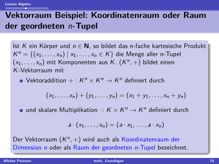
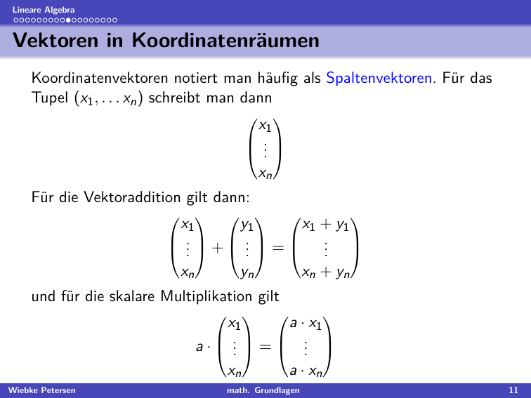
"# Vektorraum der geordneten $n$-Tupel"
]
},
{
"cell_type": "markdown",
"metadata": {},
"source": [
""
]
},
{
"cell_type": "markdown",
"metadata": {},
"source": [
"In diesem Vektorraum können wir jetzt die Addition und Multiplikation sowie das Skalarprodukt zweier Vektoren berechnen. Diese werden auf den Folien und im Video erklärt. Es gibt viele weitere Quellen und Tutorials dazu im Internet."
]
},
{
"cell_type": "markdown",
"metadata": {},
"source": [
""
]
},
{
"cell_type": "markdown",
"metadata": {},
"source": [
"# Addition, Multiplikation"
]
},
{
"cell_type": "markdown",
"metadata": {},
"source": [
""
]
},
{
"cell_type": "markdown",
"metadata": {},
"source": [
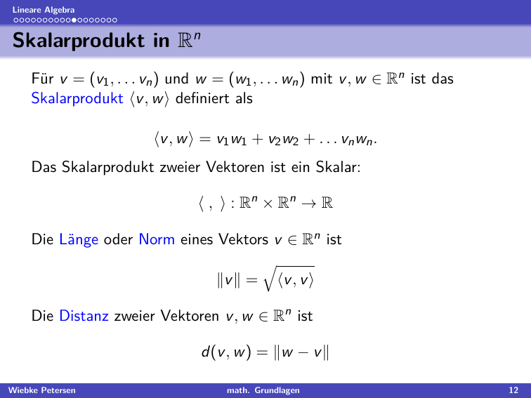
"## Skalarprodukt, Länge, Distanz "
]
},
{
"cell_type": "markdown",
"metadata": {},
"source": [
""
]
},
{
"cell_type": "markdown",
"metadata": {},
"source": [
"## Video zur Länge eines Vektors und zur Distanz zweier Vektoren"
]
},
{
"cell_type": "markdown",
"metadata": {},
"source": [
""
]
},
{
"cell_type": "markdown",
"metadata": {},
"source": [
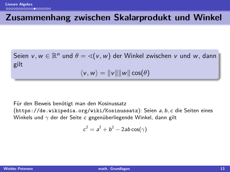
"## Zusammenhang Zwischen Skalarprodukt und Winkel "
]
},
{
"cell_type": "markdown",
"metadata": {},
"source": [
""
]
},
{
"cell_type": "markdown",
"metadata": {},
"source": [
"[Wikipedia Kosinussatz](https://de.wikipedia.org/wiki/Kosinussatz) - notwendig für den Beweis\n",
"\n",
"\n",
"Was bringt uns dieser Zusammenhang? Angenommen, wir möchten den Winkel zwischen 2 uns bekannten Vektoren $v$ und $w$ kennen. Dann setzen wir die beiden Vektoren in die Gleichung ein und finden den Cosinus des Winkels heraus. Darüber finden wir auch den Winkel selbst."
]
},
{
"cell_type": "code",
"execution_count": null,
"metadata": {},
"outputs": [],
"source": []
}
],
"metadata": {
"kernelspec": {
"display_name": "Python 3",
"language": "python",
"name": "python3"
},
"language_info": {
"codemirror_mode": {
"name": "ipython",
"version": 3
},
"file_extension": ".py",
"mimetype": "text/x-python",
"name": "python",
"nbconvert_exporter": "python",
"pygments_lexer": "ipython3",
"version": "3.6.4"
}
},
"nbformat": 4,
"nbformat_minor": 2
}