{
"cells": [
{
"cell_type": "markdown",
"metadata": {},
"source": [
"# 4 - Hybdrid Absorbing Boundary Condition (HABC)"
]
},
{
"cell_type": "markdown",
"metadata": {},
"source": [
"# 4.1 - Introduction\n",
"\n",
"In this notebook we describe absorbing boundary conditions and their use combined with the *Hybdrid Absorbing Boundary Condition* (*HABC*). The common points to the previous notebooks Introduction to Acoustic Problem, Damping and PML will be used here, with brief descriptions."
]
},
{
"cell_type": "markdown",
"metadata": {},
"source": [
"# 4.2 - Absorbing Boundary Conditions\n",
"\n",
" We initially describe absorbing boundary conditions, the so called A1 and A2 Clayton's conditions and\n",
" the scheme from Higdon. These methods can be used as pure boundary conditions, designed to reduce reflections,\n",
" or as part of the Hybrid Absorbing Boundary Condition, in which they are combined with an absorption layer in a manner to be described ahead. \n",
" \n",
" In the presentation of these boundary conditions we initially consider the wave equation to be solved on\n",
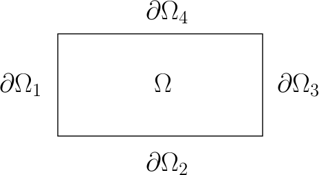
" the spatial domain $\\Omega=\\left[x_{I},x_{F}\\right] \\times\\left[z_{I},z_{F}\\right]$ as show in the figure bellow. More details about the equation and domain definition can be found in the Introduction to Acoustic Problem notebook. \n",
"\n",
" \n",
" \n",
"## 4.2.1 - Clayton's A1 Boundary Condition\n",
"\n",
"Clayton's A1 boundary condition is based on a one way wave equation (OWWE). This simple condition\n",
" is such that outgoing waves normal to the border would leave without reflection. At the $\\partial \\Omega_1$ part of the boundary\n",
" we have, \n",
"\n",
"- $\\displaystyle\\frac{\\partial u(x,z,t)}{\\partial t}-c(x,z)\\displaystyle\\frac{\\partial u(x,z,t)}{\\partial x}=0.$\n",
"\n",
"while at $\\partial \\Omega_3$ the condition is\n",
" \n",
"- $\\displaystyle\\frac{\\partial u(x,z,t)}{\\partial t}+c(x,z)\\displaystyle\\frac{\\partial u(x,z,t)}{\\partial x}=0.$\n",
"\n",
"and at $\\partial \\Omega_2$\n",
"\n",
"- $\\displaystyle\\frac{\\partial u(x,z,t)}{\\partial t}+c(x,z)\\displaystyle\\frac{\\partial u(x,z,t)}{\\partial z}=0.$\n",
"\n",
"## 4.2.2 - Clayton's A2 Boundary Condition \n",
"\n",
"The A2 boundary condition aims to impose a boundary condition that would make outgoing waves leave the domain without being reflected. This condition is approximated (using a Padé approximation in the wave dispersion relation) by the following equation to be imposed on the boundary part $\\partial \\Omega_1$\n",
"\n",
"- $\\displaystyle\\frac{\\partial^{2} u(x,z,t)}{\\partial t^{2}}+c(x,z)\\displaystyle\\frac{\\partial^{2} u(x,z,t)}{\\partial x \\partial t}+\\frac{c^2(x,z)}{2}\\displaystyle\\frac{\\partial^{2} u(x,z,t)}{\\partial z^{2}}=0.$\n",
"\n",
"At $\\partial \\Omega_3$ we have\n",
"\n",
"- $\\displaystyle\\frac{\\partial^{2} u(x,z,t)}{\\partial t^{2}}-c(x,z)\\displaystyle\\frac{\\partial^{2} u(x,z,t)}{\\partial z \\partial t}+\\frac{c^2(x,z)}{2}\\displaystyle\\frac{\\partial^{2} u(x,z,t)}{\\partial x^{2}}=0.$\n",
"\n",
"while at $\\partial \\Omega_2$ the condition is\n",
"\n",
"- $\\displaystyle\\frac{\\partial^{2} u(x,z,t)}{\\partial t^{2}}-c(x,z)\\displaystyle\\frac{\\partial^{2} u(x,z,t)}{\\partial x \\partial t}+\\frac{c^2(x,z)}{2}\\displaystyle\\frac{\\partial^{2} u(x,z,t)}{\\partial z^{2}}=0.$\n",
"\n",
"At the corner points the condition is \n",
"\n",
"- $\\displaystyle\\frac{\\sqrt{2}\\partial u(x,z,t)}{\\partial t}+c(x,z)\\left(\\displaystyle\\frac{\\partial u(x,z,t)}{\\partial x}+\\displaystyle\\frac{\\partial u(x,z,t)}{\\partial z}\\right)=0.$\n",
"\n",
"## 4.2.3 - Higdon Boundary Condition\n",
"\n",
"The Higdon Boundary condition of order p is given at $\\partial \\Omega_1$ and $\\partial \\Omega_3$n by:\n",
"\n",
"- $\\Pi_{j=1}^p(\\cos(\\alpha_j)\\left(\\displaystyle\\frac{\\partial }{\\partial t}-c(x,z)\\displaystyle\\frac{\\partial }{\\partial x}\\right)u(x,z,t)=0.$\n",
"\n",
"and at $\\partial \\Omega_2$\n",
"\n",
"- $\\Pi_{j=1}^p(\\cos(\\alpha_j)\\left(\\displaystyle\\frac{\\partial}{\\partial t}-c(x,z)\\displaystyle\\frac{\\partial}{\\partial z}\\right)u(x,z,t)=0.$\n",
"\n",
" This method would make that outgoing waves with angle of incidence at the boundary equal to $\\alpha_j$ would\n",
" present no reflection. The method we use in this notebook employs order 2 ($p=2$) and angles $0$ and $\\pi/4$.\n",
" \n",
" Observation: There are similarities between Clayton's A2 and the Higdon condition. If one chooses $p=2$ and\n",
" both angles equal to zero in Higdon's method, this leads to the condition:\n",
" $ u_{tt}-2cu_{xt}+c^2u_{xx}=0$. But, using the wave equation, we have that $c^2u_{xx}=u_{tt}-c^2u_{zz}$. Replacing this relation in the previous equation, we get: $2u_{tt}-2cu_{xt}-c^2u_{zz}=0$ which is Clayton's A2\n",
" boundary condition. In this since, Higdon's method would generalize Clayton's scheme. But the discretization of\n",
" both methods are quite different, since in Higdon's scheme the boundary operators are unidirectional, while\n",
" in Clayton's A2 not."
]
},
{
"cell_type": "markdown",
"metadata": {},
"source": [
"# 4.3 - Acoustic Problem with HABC\n",
"\n",
"In the hybrid absorption boundary condition (HABC) scheme we will also extend the spatial domain as $\\Omega=\\left[x_{I}-L,x_{F}+L\\right] \\times\\left[z_{I},z_{F}+L\\right]$.\n",
"\n",
"We added to the target domain $\\Omega_{0}=\\left[x_{I},x_{F}\\right]\\times\\left[z_{I},z_{F}\\right]$ an extension zone, of length $L$ in both ends of the direction $x$ and at the end of the domain in the direction $z$, as represented in the figure bellow.\n",
"\n",
"
\n",
" \n",
"## 4.2.1 - Clayton's A1 Boundary Condition\n",
"\n",
"Clayton's A1 boundary condition is based on a one way wave equation (OWWE). This simple condition\n",
" is such that outgoing waves normal to the border would leave without reflection. At the $\\partial \\Omega_1$ part of the boundary\n",
" we have, \n",
"\n",
"- $\\displaystyle\\frac{\\partial u(x,z,t)}{\\partial t}-c(x,z)\\displaystyle\\frac{\\partial u(x,z,t)}{\\partial x}=0.$\n",
"\n",
"while at $\\partial \\Omega_3$ the condition is\n",
" \n",
"- $\\displaystyle\\frac{\\partial u(x,z,t)}{\\partial t}+c(x,z)\\displaystyle\\frac{\\partial u(x,z,t)}{\\partial x}=0.$\n",
"\n",
"and at $\\partial \\Omega_2$\n",
"\n",
"- $\\displaystyle\\frac{\\partial u(x,z,t)}{\\partial t}+c(x,z)\\displaystyle\\frac{\\partial u(x,z,t)}{\\partial z}=0.$\n",
"\n",
"## 4.2.2 - Clayton's A2 Boundary Condition \n",
"\n",
"The A2 boundary condition aims to impose a boundary condition that would make outgoing waves leave the domain without being reflected. This condition is approximated (using a Padé approximation in the wave dispersion relation) by the following equation to be imposed on the boundary part $\\partial \\Omega_1$\n",
"\n",
"- $\\displaystyle\\frac{\\partial^{2} u(x,z,t)}{\\partial t^{2}}+c(x,z)\\displaystyle\\frac{\\partial^{2} u(x,z,t)}{\\partial x \\partial t}+\\frac{c^2(x,z)}{2}\\displaystyle\\frac{\\partial^{2} u(x,z,t)}{\\partial z^{2}}=0.$\n",
"\n",
"At $\\partial \\Omega_3$ we have\n",
"\n",
"- $\\displaystyle\\frac{\\partial^{2} u(x,z,t)}{\\partial t^{2}}-c(x,z)\\displaystyle\\frac{\\partial^{2} u(x,z,t)}{\\partial z \\partial t}+\\frac{c^2(x,z)}{2}\\displaystyle\\frac{\\partial^{2} u(x,z,t)}{\\partial x^{2}}=0.$\n",
"\n",
"while at $\\partial \\Omega_2$ the condition is\n",
"\n",
"- $\\displaystyle\\frac{\\partial^{2} u(x,z,t)}{\\partial t^{2}}-c(x,z)\\displaystyle\\frac{\\partial^{2} u(x,z,t)}{\\partial x \\partial t}+\\frac{c^2(x,z)}{2}\\displaystyle\\frac{\\partial^{2} u(x,z,t)}{\\partial z^{2}}=0.$\n",
"\n",
"At the corner points the condition is \n",
"\n",
"- $\\displaystyle\\frac{\\sqrt{2}\\partial u(x,z,t)}{\\partial t}+c(x,z)\\left(\\displaystyle\\frac{\\partial u(x,z,t)}{\\partial x}+\\displaystyle\\frac{\\partial u(x,z,t)}{\\partial z}\\right)=0.$\n",
"\n",
"## 4.2.3 - Higdon Boundary Condition\n",
"\n",
"The Higdon Boundary condition of order p is given at $\\partial \\Omega_1$ and $\\partial \\Omega_3$n by:\n",
"\n",
"- $\\Pi_{j=1}^p(\\cos(\\alpha_j)\\left(\\displaystyle\\frac{\\partial }{\\partial t}-c(x,z)\\displaystyle\\frac{\\partial }{\\partial x}\\right)u(x,z,t)=0.$\n",
"\n",
"and at $\\partial \\Omega_2$\n",
"\n",
"- $\\Pi_{j=1}^p(\\cos(\\alpha_j)\\left(\\displaystyle\\frac{\\partial}{\\partial t}-c(x,z)\\displaystyle\\frac{\\partial}{\\partial z}\\right)u(x,z,t)=0.$\n",
"\n",
" This method would make that outgoing waves with angle of incidence at the boundary equal to $\\alpha_j$ would\n",
" present no reflection. The method we use in this notebook employs order 2 ($p=2$) and angles $0$ and $\\pi/4$.\n",
" \n",
" Observation: There are similarities between Clayton's A2 and the Higdon condition. If one chooses $p=2$ and\n",
" both angles equal to zero in Higdon's method, this leads to the condition:\n",
" $ u_{tt}-2cu_{xt}+c^2u_{xx}=0$. But, using the wave equation, we have that $c^2u_{xx}=u_{tt}-c^2u_{zz}$. Replacing this relation in the previous equation, we get: $2u_{tt}-2cu_{xt}-c^2u_{zz}=0$ which is Clayton's A2\n",
" boundary condition. In this since, Higdon's method would generalize Clayton's scheme. But the discretization of\n",
" both methods are quite different, since in Higdon's scheme the boundary operators are unidirectional, while\n",
" in Clayton's A2 not."
]
},
{
"cell_type": "markdown",
"metadata": {},
"source": [
"# 4.3 - Acoustic Problem with HABC\n",
"\n",
"In the hybrid absorption boundary condition (HABC) scheme we will also extend the spatial domain as $\\Omega=\\left[x_{I}-L,x_{F}+L\\right] \\times\\left[z_{I},z_{F}+L\\right]$.\n",
"\n",
"We added to the target domain $\\Omega_{0}=\\left[x_{I},x_{F}\\right]\\times\\left[z_{I},z_{F}\\right]$ an extension zone, of length $L$ in both ends of the direction $x$ and at the end of the domain in the direction $z$, as represented in the figure bellow.\n",
"\n",
" \n",
"\n",
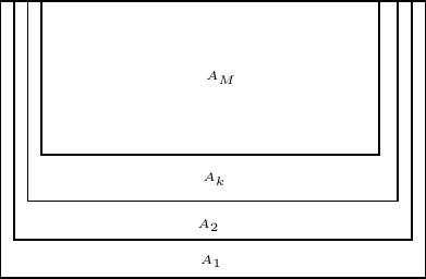
" The difference with respect to previous schemes, is that this extended region will now be considered as the union of several gradual extensions. As represented in the next figure, we define a region $A_M=\\Omega_{0}$. The regions $A_k, k=M-1,\\cdots,1$ will be defined as the previous region $A_{k+1}$ to which we add one extra grid line to the left,\n",
" right and bottom sides of it, such that the final region $A_1=\\Omega$ (we thus have $M=L+1$).\n",
" \n",
"
\n",
"\n",
" The difference with respect to previous schemes, is that this extended region will now be considered as the union of several gradual extensions. As represented in the next figure, we define a region $A_M=\\Omega_{0}$. The regions $A_k, k=M-1,\\cdots,1$ will be defined as the previous region $A_{k+1}$ to which we add one extra grid line to the left,\n",
" right and bottom sides of it, such that the final region $A_1=\\Omega$ (we thus have $M=L+1$).\n",
" \n",
"  \n",
" \n",
" We now consider the temporal evolution\n",
" of the solution of the HABC method. Suppose that $u(x,z,t-1)$ is the solution at a given instant $t-1$ in all the \n",
" extended $\\Omega$ domain. We update it to instant $t$, using one of the absorbing boundary conditions described in the previous section (A1, A2 or Higdon) producing a preliminar new function $u(x,z,t)$. Now, call $u_{1}(x,z,t)$ the solution at instant $t$ constructed in the extended region, by applying the same absorbing boundary condition at the border of each of the domains $A_k,k=1,..,M$. The HABC solution will be constructed as a convex combination of $u(x,z,t)$ and $u_{1}(x,z,t)$:\n",
" \n",
"- $u(x,z,t) = (1-\\omega)u(x,z,t)+\\omega u_{1}(x,z,t)$.\n",
"\n",
"The function $u_{1}(x,z,t)$ is defined (and used) only in the extension of the domain. The function $w$ is a \n",
"weight function growing from zero at the boundary $\\partial\\Omega_{0}$ to one at $\\partial\\Omega$. The particular weight function to be used could vary linearly, as when the scheme was first proposed by Liu and Sen. But HABC produces better results with a non-linear weight function to be described ahead.\n",
"\n",
"The wave equation employed here will be the same as in the previous notebooks, with same velocity model, source term and initial conditions.\n",
"\n"
]
},
{
"cell_type": "markdown",
"metadata": {},
"source": [
"## 4.3.1 The weight function $\\omega$\n",
"\n",
"One can choose a *linear* weight function as \n",
"\n",
"\\begin{equation}\n",
"\\omega_{k} = \\displaystyle\\frac{M-k}{M};\n",
"\\end{equation}\n",
"\n",
"or preferably a *non linear*\n",
"\n",
"\\begin{equation}\n",
"\\omega_{k}=\\left\\{ \\begin{array}{ll}\n",
"1, & \\textrm{if $1\\leq k \\leq P+1$,} \\\\ \\left(\\displaystyle\\frac{M-k}{M-P}\\right)^{\\alpha} , & \\textrm{if $P+2 \\leq k \\leq M-1.$} \\\\ 0 , & \\textrm{if $k=M$.}\\end{array}\\right.\n",
"\\label{eq:elo8}\n",
"\\end{equation} \n",
"\n",
"In general we take $P=2$ and we choose $\\alpha$ as follows:\n",
"\n",
"- $\\alpha = 1.5 + 0.07(npt-P)$, in the case of A1 and A2;\n",
"- $\\alpha = 1.0 + 0.15(npt-P)$, in the case of Higdon.\n",
"\n",
"The value *npt* designates the number of discrete points that define the length of the blue band in the direction $x$ and/or $z$."
]
},
{
"cell_type": "markdown",
"metadata": {},
"source": [
"# 4.4 - Finite Difference Operators and Discretization of Spatial and Temporal Domains\n",
"\n",
" We employ the same methods as in the previous notebooks. "
]
},
{
"cell_type": "markdown",
"metadata": {},
"source": [
"# 4.5 - Standard Problem\n",
"\n",
"Redeeming the Standard Problem definitions discussed on the notebook Introduction to Acoustic Problem we have that:\n",
"\n",
"- $x_{I}$ = 0.0 Km;\n",
"- $x_{F}$ = 1.0 Km = 1000 m;\n",
"- $z_{I}$ = 0.0 Km;\n",
"- $z_{F}$ = 1.0 Km = 1000 m;\n",
"\n",
"The spatial discretization parameters are given by:\n",
"- $\\Delta x$ = 0.01 km = 10m;\n",
"- $\\Delta z$ = 0.01 km = 10m;\n",
"\n",
"Let's consider a $I$ the time domain with the following limitations:\n",
"\n",
"- $t_{I}$ = 0 s = 0 ms;\n",
"- $t_{F}$ = 1 s = 1000 ms;\n",
"\n",
"The temporal discretization parameters are given by:\n",
"\n",
"- $\\Delta t$ $\\approx$ 0.0016 s = 1.6 ms;\n",
"- $NT$ = 626.\n",
"\n",
"The source term, velocity model and positioning of receivers will be as in the previous notebooks."
]
},
{
"cell_type": "markdown",
"metadata": {},
"source": [
"# 4.6 - Numerical Simulations\n",
"\n",
"For the numerical simulations of this notebook we use several of the notebook codes presented in Damping e PML. The new features will be described in more detail.\n",
"\n",
"So, we import the following Python and Devito packages:"
]
},
{
"cell_type": "code",
"execution_count": 1,
"metadata": {},
"outputs": [],
"source": [
"# NBVAL_IGNORE_OUTPUT\n",
"\n",
"import numpy as np\n",
"import matplotlib.pyplot as plot\n",
"import matplotlib.ticker as mticker\n",
"from mpl_toolkits.axes_grid1 import make_axes_locatable\n",
"from matplotlib import cm"
]
},
{
"cell_type": "markdown",
"metadata": {},
"source": [
"From Devito's library of examples we import the following structures:"
]
},
{
"cell_type": "code",
"execution_count": 2,
"metadata": {},
"outputs": [],
"source": [
"# NBVAL_IGNORE_OUTPUT\n",
"\n",
"%matplotlib inline\n",
"from examples.seismic import TimeAxis\n",
"from examples.seismic import RickerSource\n",
"from examples.seismic import Receiver\n",
"from devito import SubDomain, Grid, NODE, TimeFunction, Function, Eq, solve, Operator"
]
},
{
"cell_type": "markdown",
"metadata": {},
"source": [
"The mesh parameters that we choose define the domain $\\Omega_{0}$ plus the absorption region. For this, we use the following data:"
]
},
{
"cell_type": "code",
"execution_count": 3,
"metadata": {},
"outputs": [],
"source": [
"nptx = 101\n",
"nptz = 101\n",
"x0 = 0.\n",
"x1 = 1000.\n",
"compx = x1-x0\n",
"z0 = 0.\n",
"z1 = 1000.\n",
"compz = z1-z0\n",
"hxv = (x1-x0)/(nptx-1)\n",
"hzv = (z1-z0)/(nptz-1)"
]
},
{
"cell_type": "markdown",
"metadata": {},
"source": [
"As we saw previously, HABC has three approach possibilities (A1, A2 and Higdon) and two types of weights (linear and non-linear). So, we insert two control variables. The variable called *habctype* chooses the type of HABC approach and is such that:\n",
"\n",
"- *habctype=1* is equivalent to choosing A1;\n",
"- *habctype=2* is equivalent to choosing A2;\n",
"- *habctype=3* is equivalent to choosing Higdon;\n",
"\n",
"Regarding the weights, we will introduce the variable *habcw* that chooses the type of weight and is such that:\n",
"\n",
"- *habcw=1* is equivalent to linear weight;\n",
"- *habcw=2* is equivalent to non-linear weights;\n",
"\n",
"In this way, we make the following choices:"
]
},
{
"cell_type": "code",
"execution_count": 4,
"metadata": {},
"outputs": [],
"source": [
"habctype = 3\n",
"habcw = 2"
]
},
{
"cell_type": "markdown",
"metadata": {},
"source": [
"The number of points of the absorption layer in the directions $x$ and $z$ are given, respectively, by:"
]
},
{
"cell_type": "code",
"execution_count": 5,
"metadata": {},
"outputs": [],
"source": [
"npmlx = 20\n",
"npmlz = 20"
]
},
{
"cell_type": "markdown",
"metadata": {},
"source": [
"The lengths $L_{x}$ and $L_{z}$ are given, respectively, by:"
]
},
{
"cell_type": "code",
"execution_count": 6,
"metadata": {},
"outputs": [],
"source": [
"lx = npmlx*hxv\n",
"lz = npmlz*hzv"
]
},
{
"cell_type": "markdown",
"metadata": {},
"source": [
"For the construction of the *grid* we have:"
]
},
{
"cell_type": "code",
"execution_count": 7,
"metadata": {},
"outputs": [],
"source": [
"nptx = nptx + 2*npmlx\n",
"nptz = nptz + 1*npmlz\n",
"x0 = x0 - hxv*npmlx\n",
"x1 = x1 + hxv*npmlx\n",
"compx = x1-x0\n",
"z0 = z0\n",
"z1 = z1 + hzv*npmlz\n",
"compz = z1-z0\n",
"origin = (x0, z0)\n",
"extent = (compx, compz)\n",
"shape = (nptx, nptz)\n",
"spacing = (hxv, hzv)"
]
},
{
"cell_type": "markdown",
"metadata": {},
"source": [
"As in the case of the acoustic equation with Damping and in the acoustic equation with PML, we can define specific regions in our domain, since the solution $u_{1}(x,z,t)$ is only calculated in the blue region. We will soon follow a similar scheme for creating *subdomains* as was done on notebooks Damping and PML.\n",
"\n",
"First, we define a region corresponding to the entire domain, naming this region as *d0*. In the language of *subdomains* *d0* it is written as:"
]
},
{
"cell_type": "code",
"execution_count": 8,
"metadata": {},
"outputs": [],
"source": [
"class d0domain(SubDomain):\n",
" name = 'd0'\n",
"\n",
" def define(self, dimensions):\n",
" x, z = dimensions\n",
" return {x: x, z: z}\n",
"\n",
"\n",
"d0_domain = d0domain()"
]
},
{
"cell_type": "markdown",
"metadata": {},
"source": [
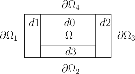
"The blue region will be built with 3 divisions:\n",
"\n",
"- *d1* represents the left range in the direction *x*, where the pairs $(x,z)$ satisfy: $x\\in\\{0,npmlx\\}$ and $z\\in\\{0,nptz\\}$;\n",
"- *d2* represents the right range in the direction *x*, where the pairs $(x,z)$ satisfy: $x\\in\\{nptx-npmlx,nptx\\}$ and $z\\in\\{0,nptz\\}$;\n",
"- *d3* represents the left range in the direction *y*, where the pairs $(x,z)$ satisfy: $x\\in\\{npmlx,nptx-npmlx\\}$ and $z\\in\\{nptz-npmlz,nptz\\}$;\n",
"\n",
"Thus, the regions *d1*, *d2* and *d3* are described as follows in the language of *subdomains*:"
]
},
{
"cell_type": "code",
"execution_count": 9,
"metadata": {},
"outputs": [],
"source": [
"class d1domain(SubDomain):\n",
" name = 'd1'\n",
"\n",
" def define(self, dimensions):\n",
" x, z = dimensions\n",
" return {x: ('left', npmlx), z: z}\n",
"\n",
"\n",
"d1_domain = d1domain()\n",
"\n",
"\n",
"class d2domain(SubDomain):\n",
" name = 'd2'\n",
"\n",
" def define(self, dimensions):\n",
" x, z = dimensions\n",
" return {x: ('right', npmlx), z: z}\n",
"\n",
"\n",
"d2_domain = d2domain()\n",
"\n",
"\n",
"class d3domain(SubDomain):\n",
" name = 'd3'\n",
"\n",
" def define(self, dimensions):\n",
" x, z = dimensions\n",
" if((habctype == 3) & (habcw == 1)):\n",
" return {x: x, z: ('right', npmlz)}\n",
" else:\n",
" return {x: ('middle', npmlx, npmlx), z: ('right', npmlz)}\n",
"\n",
"\n",
"d3_domain = d3domain()"
]
},
{
"cell_type": "markdown",
"metadata": {},
"source": [
"The figure below represents the division of domains that we did previously:\n",
"\n",
"
\n",
" \n",
" We now consider the temporal evolution\n",
" of the solution of the HABC method. Suppose that $u(x,z,t-1)$ is the solution at a given instant $t-1$ in all the \n",
" extended $\\Omega$ domain. We update it to instant $t$, using one of the absorbing boundary conditions described in the previous section (A1, A2 or Higdon) producing a preliminar new function $u(x,z,t)$. Now, call $u_{1}(x,z,t)$ the solution at instant $t$ constructed in the extended region, by applying the same absorbing boundary condition at the border of each of the domains $A_k,k=1,..,M$. The HABC solution will be constructed as a convex combination of $u(x,z,t)$ and $u_{1}(x,z,t)$:\n",
" \n",
"- $u(x,z,t) = (1-\\omega)u(x,z,t)+\\omega u_{1}(x,z,t)$.\n",
"\n",
"The function $u_{1}(x,z,t)$ is defined (and used) only in the extension of the domain. The function $w$ is a \n",
"weight function growing from zero at the boundary $\\partial\\Omega_{0}$ to one at $\\partial\\Omega$. The particular weight function to be used could vary linearly, as when the scheme was first proposed by Liu and Sen. But HABC produces better results with a non-linear weight function to be described ahead.\n",
"\n",
"The wave equation employed here will be the same as in the previous notebooks, with same velocity model, source term and initial conditions.\n",
"\n"
]
},
{
"cell_type": "markdown",
"metadata": {},
"source": [
"## 4.3.1 The weight function $\\omega$\n",
"\n",
"One can choose a *linear* weight function as \n",
"\n",
"\\begin{equation}\n",
"\\omega_{k} = \\displaystyle\\frac{M-k}{M};\n",
"\\end{equation}\n",
"\n",
"or preferably a *non linear*\n",
"\n",
"\\begin{equation}\n",
"\\omega_{k}=\\left\\{ \\begin{array}{ll}\n",
"1, & \\textrm{if $1\\leq k \\leq P+1$,} \\\\ \\left(\\displaystyle\\frac{M-k}{M-P}\\right)^{\\alpha} , & \\textrm{if $P+2 \\leq k \\leq M-1.$} \\\\ 0 , & \\textrm{if $k=M$.}\\end{array}\\right.\n",
"\\label{eq:elo8}\n",
"\\end{equation} \n",
"\n",
"In general we take $P=2$ and we choose $\\alpha$ as follows:\n",
"\n",
"- $\\alpha = 1.5 + 0.07(npt-P)$, in the case of A1 and A2;\n",
"- $\\alpha = 1.0 + 0.15(npt-P)$, in the case of Higdon.\n",
"\n",
"The value *npt* designates the number of discrete points that define the length of the blue band in the direction $x$ and/or $z$."
]
},
{
"cell_type": "markdown",
"metadata": {},
"source": [
"# 4.4 - Finite Difference Operators and Discretization of Spatial and Temporal Domains\n",
"\n",
" We employ the same methods as in the previous notebooks. "
]
},
{
"cell_type": "markdown",
"metadata": {},
"source": [
"# 4.5 - Standard Problem\n",
"\n",
"Redeeming the Standard Problem definitions discussed on the notebook Introduction to Acoustic Problem we have that:\n",
"\n",
"- $x_{I}$ = 0.0 Km;\n",
"- $x_{F}$ = 1.0 Km = 1000 m;\n",
"- $z_{I}$ = 0.0 Km;\n",
"- $z_{F}$ = 1.0 Km = 1000 m;\n",
"\n",
"The spatial discretization parameters are given by:\n",
"- $\\Delta x$ = 0.01 km = 10m;\n",
"- $\\Delta z$ = 0.01 km = 10m;\n",
"\n",
"Let's consider a $I$ the time domain with the following limitations:\n",
"\n",
"- $t_{I}$ = 0 s = 0 ms;\n",
"- $t_{F}$ = 1 s = 1000 ms;\n",
"\n",
"The temporal discretization parameters are given by:\n",
"\n",
"- $\\Delta t$ $\\approx$ 0.0016 s = 1.6 ms;\n",
"- $NT$ = 626.\n",
"\n",
"The source term, velocity model and positioning of receivers will be as in the previous notebooks."
]
},
{
"cell_type": "markdown",
"metadata": {},
"source": [
"# 4.6 - Numerical Simulations\n",
"\n",
"For the numerical simulations of this notebook we use several of the notebook codes presented in Damping e PML. The new features will be described in more detail.\n",
"\n",
"So, we import the following Python and Devito packages:"
]
},
{
"cell_type": "code",
"execution_count": 1,
"metadata": {},
"outputs": [],
"source": [
"# NBVAL_IGNORE_OUTPUT\n",
"\n",
"import numpy as np\n",
"import matplotlib.pyplot as plot\n",
"import matplotlib.ticker as mticker\n",
"from mpl_toolkits.axes_grid1 import make_axes_locatable\n",
"from matplotlib import cm"
]
},
{
"cell_type": "markdown",
"metadata": {},
"source": [
"From Devito's library of examples we import the following structures:"
]
},
{
"cell_type": "code",
"execution_count": 2,
"metadata": {},
"outputs": [],
"source": [
"# NBVAL_IGNORE_OUTPUT\n",
"\n",
"%matplotlib inline\n",
"from examples.seismic import TimeAxis\n",
"from examples.seismic import RickerSource\n",
"from examples.seismic import Receiver\n",
"from devito import SubDomain, Grid, NODE, TimeFunction, Function, Eq, solve, Operator"
]
},
{
"cell_type": "markdown",
"metadata": {},
"source": [
"The mesh parameters that we choose define the domain $\\Omega_{0}$ plus the absorption region. For this, we use the following data:"
]
},
{
"cell_type": "code",
"execution_count": 3,
"metadata": {},
"outputs": [],
"source": [
"nptx = 101\n",
"nptz = 101\n",
"x0 = 0.\n",
"x1 = 1000.\n",
"compx = x1-x0\n",
"z0 = 0.\n",
"z1 = 1000.\n",
"compz = z1-z0\n",
"hxv = (x1-x0)/(nptx-1)\n",
"hzv = (z1-z0)/(nptz-1)"
]
},
{
"cell_type": "markdown",
"metadata": {},
"source": [
"As we saw previously, HABC has three approach possibilities (A1, A2 and Higdon) and two types of weights (linear and non-linear). So, we insert two control variables. The variable called *habctype* chooses the type of HABC approach and is such that:\n",
"\n",
"- *habctype=1* is equivalent to choosing A1;\n",
"- *habctype=2* is equivalent to choosing A2;\n",
"- *habctype=3* is equivalent to choosing Higdon;\n",
"\n",
"Regarding the weights, we will introduce the variable *habcw* that chooses the type of weight and is such that:\n",
"\n",
"- *habcw=1* is equivalent to linear weight;\n",
"- *habcw=2* is equivalent to non-linear weights;\n",
"\n",
"In this way, we make the following choices:"
]
},
{
"cell_type": "code",
"execution_count": 4,
"metadata": {},
"outputs": [],
"source": [
"habctype = 3\n",
"habcw = 2"
]
},
{
"cell_type": "markdown",
"metadata": {},
"source": [
"The number of points of the absorption layer in the directions $x$ and $z$ are given, respectively, by:"
]
},
{
"cell_type": "code",
"execution_count": 5,
"metadata": {},
"outputs": [],
"source": [
"npmlx = 20\n",
"npmlz = 20"
]
},
{
"cell_type": "markdown",
"metadata": {},
"source": [
"The lengths $L_{x}$ and $L_{z}$ are given, respectively, by:"
]
},
{
"cell_type": "code",
"execution_count": 6,
"metadata": {},
"outputs": [],
"source": [
"lx = npmlx*hxv\n",
"lz = npmlz*hzv"
]
},
{
"cell_type": "markdown",
"metadata": {},
"source": [
"For the construction of the *grid* we have:"
]
},
{
"cell_type": "code",
"execution_count": 7,
"metadata": {},
"outputs": [],
"source": [
"nptx = nptx + 2*npmlx\n",
"nptz = nptz + 1*npmlz\n",
"x0 = x0 - hxv*npmlx\n",
"x1 = x1 + hxv*npmlx\n",
"compx = x1-x0\n",
"z0 = z0\n",
"z1 = z1 + hzv*npmlz\n",
"compz = z1-z0\n",
"origin = (x0, z0)\n",
"extent = (compx, compz)\n",
"shape = (nptx, nptz)\n",
"spacing = (hxv, hzv)"
]
},
{
"cell_type": "markdown",
"metadata": {},
"source": [
"As in the case of the acoustic equation with Damping and in the acoustic equation with PML, we can define specific regions in our domain, since the solution $u_{1}(x,z,t)$ is only calculated in the blue region. We will soon follow a similar scheme for creating *subdomains* as was done on notebooks Damping and PML.\n",
"\n",
"First, we define a region corresponding to the entire domain, naming this region as *d0*. In the language of *subdomains* *d0* it is written as:"
]
},
{
"cell_type": "code",
"execution_count": 8,
"metadata": {},
"outputs": [],
"source": [
"class d0domain(SubDomain):\n",
" name = 'd0'\n",
"\n",
" def define(self, dimensions):\n",
" x, z = dimensions\n",
" return {x: x, z: z}\n",
"\n",
"\n",
"d0_domain = d0domain()"
]
},
{
"cell_type": "markdown",
"metadata": {},
"source": [
"The blue region will be built with 3 divisions:\n",
"\n",
"- *d1* represents the left range in the direction *x*, where the pairs $(x,z)$ satisfy: $x\\in\\{0,npmlx\\}$ and $z\\in\\{0,nptz\\}$;\n",
"- *d2* represents the right range in the direction *x*, where the pairs $(x,z)$ satisfy: $x\\in\\{nptx-npmlx,nptx\\}$ and $z\\in\\{0,nptz\\}$;\n",
"- *d3* represents the left range in the direction *y*, where the pairs $(x,z)$ satisfy: $x\\in\\{npmlx,nptx-npmlx\\}$ and $z\\in\\{nptz-npmlz,nptz\\}$;\n",
"\n",
"Thus, the regions *d1*, *d2* and *d3* are described as follows in the language of *subdomains*:"
]
},
{
"cell_type": "code",
"execution_count": 9,
"metadata": {},
"outputs": [],
"source": [
"class d1domain(SubDomain):\n",
" name = 'd1'\n",
"\n",
" def define(self, dimensions):\n",
" x, z = dimensions\n",
" return {x: ('left', npmlx), z: z}\n",
"\n",
"\n",
"d1_domain = d1domain()\n",
"\n",
"\n",
"class d2domain(SubDomain):\n",
" name = 'd2'\n",
"\n",
" def define(self, dimensions):\n",
" x, z = dimensions\n",
" return {x: ('right', npmlx), z: z}\n",
"\n",
"\n",
"d2_domain = d2domain()\n",
"\n",
"\n",
"class d3domain(SubDomain):\n",
" name = 'd3'\n",
"\n",
" def define(self, dimensions):\n",
" x, z = dimensions\n",
" if((habctype == 3) & (habcw == 1)):\n",
" return {x: x, z: ('right', npmlz)}\n",
" else:\n",
" return {x: ('middle', npmlx, npmlx), z: ('right', npmlz)}\n",
"\n",
"\n",
"d3_domain = d3domain()"
]
},
{
"cell_type": "markdown",
"metadata": {},
"source": [
"The figure below represents the division of domains that we did previously:\n",
"\n",
" \n",
"\n",
"After we defining the spatial parameters and constructing the *subdomains*, we then generate the *spatial grid* and set the velocity field:"
]
},
{
"cell_type": "code",
"execution_count": 10,
"metadata": {},
"outputs": [],
"source": [
"grid = Grid(\n",
" origin=origin,\n",
" extent=extent,\n",
" shape=shape,\n",
" subdomains=(d0_domain, d1_domain, d2_domain, d3_domain),\n",
" dtype=np.float64\n",
")"
]
},
{
"cell_type": "code",
"execution_count": 11,
"metadata": {},
"outputs": [],
"source": [
"v0 = np.zeros((nptx, nptz))\n",
"X0 = np.linspace(x0, x1, nptx)\n",
"Z0 = np.linspace(z0, z1, nptz)\n",
"\n",
"x10 = x0+lx\n",
"x11 = x1-lx\n",
"\n",
"z10 = z0\n",
"z11 = z1 - lz\n",
"\n",
"xm = 0.5*(x10+x11)\n",
"zm = 0.5*(z10+z11)\n",
"\n",
"pxm = 0\n",
"pzm = 0\n",
"\n",
"for i in range(0, nptx):\n",
" if(X0[i] == xm):\n",
" pxm = i\n",
"\n",
"for j in range(0, nptz):\n",
" if(Z0[j] == zm):\n",
" pzm = j\n",
"\n",
"p0 = 0\n",
"p1 = pzm\n",
"p2 = nptz\n",
"\n",
"v0[0:nptx, p0:p1] = 1.5\n",
"v0[0:nptx, p1:p2] = 2.5"
]
},
{
"cell_type": "markdown",
"metadata": {},
"source": [
"Previously we introduce the local variables *x10,x11,z10,z11,xm,zm,pxm* and *pzm* that help us to create a specific velocity field, where we consider the whole domain (including the absorpion region). Below we include a routine to plot the velocity field."
]
},
{
"cell_type": "code",
"execution_count": 12,
"metadata": {},
"outputs": [],
"source": [
"def graph2dvel(vel):\n",
" plot.figure()\n",
" plot.figure(figsize=(16, 8))\n",
" fscale = 1/10**(3)\n",
" scale = np.amax(vel[npmlx:-npmlx, 0:-npmlz])\n",
" extent = [fscale*(x0+lx), fscale*(x1-lx), fscale*(z1-lz), fscale*(z0)]\n",
" fig = plot.imshow(\n",
" np.transpose(vel[npmlx:-npmlx, 0:-npmlz]),\n",
" vmin=0.,\n",
" vmax=scale,\n",
" cmap=cm.seismic,\n",
" extent=extent\n",
" )\n",
" plot.gca().xaxis.set_major_formatter(mticker.FormatStrFormatter('%.1f km'))\n",
" plot.gca().yaxis.set_major_formatter(mticker.FormatStrFormatter('%.1f km'))\n",
" plot.title('Velocity Profile')\n",
" plot.grid()\n",
" ax = plot.gca()\n",
" divider = make_axes_locatable(ax)\n",
" cax = divider.append_axes(\"right\", size=\"5%\", pad=0.05)\n",
" cbar = plot.colorbar(fig, cax=cax, format='%.2e')\n",
" cbar.set_label('Velocity [km/s]')\n",
" plot.show()"
]
},
{
"cell_type": "markdown",
"metadata": {},
"source": [
"Below we include the plot of velocity field."
]
},
{
"cell_type": "code",
"execution_count": 13,
"metadata": {},
"outputs": [
{
"data": {
"text/plain": [
""
]
},
"metadata": {},
"output_type": "display_data"
},
{
"data": {
"image/png": "iVBORw0KGgoAAAANSUhEUgAAA4gAAAK2CAYAAAAMt7KnAAAAOnRFWHRTb2Z0d2FyZQBNYXRwbG90bGliIHZlcnNpb24zLjEwLjMsIGh0dHBzOi8vbWF0cGxvdGxpYi5vcmcvZiW1igAAAAlwSFlzAAAPYQAAD2EBqD+naQAAm4NJREFUeJzs3XlcVPX+x/H3gIJs4oL7noaWeilzK7RS0hLTVFzSXEhNrcy1ruLNxBZt0Z9r5ZpLWiaguFaKWYqWSpiplUtq7pVwRRRFgfn9ITNXnEFnWAYaXs/HYx4P55zvNnPOvc2Hz/d8vwaj0WgUAAAAAKDIcynoAQAAAAAACgcCRAAAAACAJAJEAAAAAEAmAkQAAAAAgCQCRAAAAABAJgJEAAAAAIAkAkQAAAAAQCYCRAAAAACAJAJEAAAAAEAmAkQATmHgwIEyGAwyGAz6/fffba6Xnp6uSpUqyWAw6IEHHsiTsZjGsXjx4jxpL6+EhobKYDDo8ccfL+ih3NHixYvN3+GtLxcXF5UqVUqNGjXSqFGjdPTo0YIeqiQpPj5ePXr0UNWqVeXm5mYe74kTJyRJNWvWlMFgUHh4uEXd8PBwGQwG1axZ06FjBgAgOwSIAJxCv379zP9etmyZzfU2bdqk8+fPW7RR1Hz77bcWgU1hYzQalZSUpL1792ratGlq0KCBFi1aVKBjio+PV2BgoFauXKkzZ87oxo0bBToeAAByiwARgFNo0aKF7rnnHkn2BYhLly6VJBUrVkzPPfdcvowNObdx40YlJycrOTlZSUlJOnTokN555x25u7srNTVVL7zwgnbu3Flg45syZYquXbumChUqaMuWLfr777/N461Ro0aBjQsAgJwiQATgFAwGg/r27StJOnr0qE1Bw6VLl7RmzRpJ0lNPPaXy5cvn6xgL2uLFi2U0GvXtt98W9FBs5uHhIW9vb3l7e6tkyZLy9/fXuHHjNHfuXEk3pwhPmjSpwMa3b98+SdKzzz6r1q1by8/Pzzxeg8EgSTpx4oSMRqPVKaYAABQ2BIgAnEbfvn3NP8o//fTTu5aPiIjQ1atXzXXxz9G3b1/VqlVLkrR161alp6cXyDhSUlIkSaVKlSqQ/gEAyGsEiACcRq1atdSyZUtJ0sqVK3X9+vU7ljcFkaVLl1bHjh0tzq9Zs0Zdu3ZVtWrVVKJECZUuXVrNmzfXBx98YA4McurkyZMaOXKk6tevLx8fH3l6euree+/VkCFD9Ntvv9nUxo4dO9S/f3/de++98vb2lo+Pj+677z716NFDkZGRSk1NzVI+u0VqDAaDWrVqZX5fq1YtiwViTpw4oW3btpnff/XVV3ccW0pKikqWLCmDwaB///vftn0pdjAYDLr//vvNfSUmJkq6ma0zjfHbb7/VtWvX9P7776tJkyYqXbq01cWD7L0Wt/Zhel5z4sSJWb6vW7OFd1qkxlY//fSTBg0aJH9/f3l7e8vLy0v333+/Ro0apTNnzuS4XQAAblesoAcAAHmpX79+2rZtmxITE7V+/Xp16dLFark//vhD27ZtkyT16NFD7u7u5nNJSUnq3r27Nm3alKVOamqqdu3apV27dmn+/Pn66quvzM892iMyMlJ9+vTRtWvXshw/evSojh49qgULFmjGjBl6+eWXrda/du2aBg0aZDVL+ttvv+m3337TypUrtXXr1jxdsfTRRx+Vv7+/Dh8+rE8++URPPfVUtmUjIyOVnJwsSerfv3+ejeFWLi7/+xun0Wi0OJ+YmKhmzZrp559/zraN3F6L/GY0GjV27Fh98MEHFp/x119/1a+//qr58+dr5cqVateuXYGMEQDgXMggAnAq3bp1k6enp6Q7TzP99NNPzT+4b129NC0tTe3bt9emTZvk5eWlCRMmaO/evUpISNDJkyf1ySefqHLlyjpy5IiefvppuzOJO3fu1LPPPqtr166pcuXKWrRokU6fPq3z588rMjJS/v7+Sk9P19ChQ7Vq1SqrbfTu3dv82YKCgrRu3TqdOXNGCQkJ2rdvn2bNmqWmTZvaPKbk5GRt3LjR/P7gwYPmhVZuX3BlwIABkqS1a9eas3bWfPLJJ5KkRx55RPXq1bN5LPb45ZdfJEklSpRQ2bJlLc4PHz5chw8f1sSJE/Xrr7/qwoUL2r17t/m7yem1qFGjhvl7qV69uiQpLCwsy/c1bty4PPmMYWFhev/99yXdnFb73Xff6a+//tJff/2ljRs3qlmzZrp8+bK6du2qgwcP5kmfAIAizggATua5554zSjK6ubkZExISrJbx9/c3SjL6+/tnOT5t2jSjJKOXl5dx7969VuuePHnS6OfnZ5RknDJlisV5SUZJxkWLFlmce/DBB42SjKVLlzYeP37c4vyFCxeMtWrVMkoyVqpUyXj9+vUs57/44gtz+y+//LIxIyPD+pdgNBpv3LiR5X2/fv2MkoyPPfaYRdmtW7ea27U2LpPz588bixcvbpRknDlzptUyv//+u9FgMBglGRcsWJBtW9lZtGiReSxbt261Wubzzz83l2nbtq35+PHjx83HJRk3bNiQbT+5vRZGo9FYo0YNoyTjhAkTsu3nTmUmTJhglGSsUaOGxbkff/zR/D3OmzfPatvXr183tmjRwijJ+PTTT2c7BgAAbEUGEYDTMWUEr1+/rhUrVlic/+GHH3T48GFJlovTzJgxQ5I0YsQIPfDAA1bbr1atmoYOHSpJWr58uc3j+vHHH7V3715J0rhx46xujl62bFlNnjxZknTu3DmtX78+y/np06dLuvlc27Rp08yL8lhTrFjeP0VQoUIFdejQQdL/soS3M62W6u3trR49euRZ30ajUefOndOsWbM0cOBASTefRRwzZozV8k899ZSCg4OtnsuLa5HfZs6cKaPRqMDAQL3wwgtWyxQvXlxvv/22pJtbgly8eNGBIwQAOCMCRABOJygoSFWqVJFkfZqp6ZjBYFCfPn3Mx48ePWpedKR169a6fPlytq+GDRtKurnNwd0WwzHZvn27+d/du3fPtlynTp3k5uZmUSc5OVm7d++WJPXq1UvFixe3qd+8ZgrOfvrpJ3OQZZKRkaElS5ZIujnd19vbO1d9tWrVyrzwi4uLiypXrqxhw4bpypUrcnV11bRp09S6dWurddu3b59tu7m9Fo4QExMjSWrTps0d70XTYj0ZGRn68ccfHTpGAIDzIUAE4HRcXFzMgd8PP/ygo0ePms9dv35dX3zxhaSbwYfpGTJJWVasDAoKko+PT7avkJAQSTd/lN/pWbxb/fHHH5IkLy+vLP3ezt3dXXXq1JEkc8Bq+rdpO4fsspuO8OSTT6patWqSLLOIW7Zs0cmTJyXlz+I0rq6uql27tgYMGKAff/xRw4cPz7bsnRYQyu21yG+XL182r04aHh5+x3vx1v07//77b4eNEQDgnAgQATilWxeeWbp0qfnfGzZsUEJCgkUZ6ebqpTlx+wqY2TGt6unj43PXsqYypjqSdOnSJYvzBcHFxUXPP/+8JOmzzz7Lsp2GKWCsW7euWrRokeu+Nm7caF745cqVK0pLSzOvLhoQEHDHuqbFiqzJ7bXIb/l9LwIAkB0CRABOqV69eubVKpctW2ZesdQULHp7e5uzgCa3Tof8+eefZTQabXpZe37NGlOgcfny5buWNZW5NYApWbKk+d+ODFas6d+/v1xcXJSYmKg1a9ZIki5evKjo6GhJMgeQueXh4SFvb295e3vfMeCzV26vRX679V40PYtoyys0NNRhYwQAOCcCRABOy5QhPH78uHbs2KGEhATzdg5dunSRl5dXlvK3Tkn8/fff83w8pkDy8uXL5mmY1ly/fl1HjhzJUsf0b1dXV0k3n/8rSDVq1FCbNm0k/S9r+Pnnn+vatWsqVqyYRXa2sMnttchvvr6+5q078uNeBAAgOwSIAJzWs88+a15gZOnSpfriiy/MC8pYC2AaNGigypUrS5LV1U9zq2XLluZ/R0ZGZltuzZo15nHeWsfHx0fNmzeXdDMYu3HjRp6N7dYFb0zPOd6NabGazZs36/Tp0+ZAsV27dqpYsWKejS0/5PZaOELbtm0lSatWrbJ5ISQAAHKLABGA0ypTpox5S4aIiAgtXLhQklS9enW1atXKorzBYNCoUaMkSStXrrzrFhbp6elZFsC5m0aNGunBBx+UJE2aNMlq5ioxMVFhYWGSpEqVKunpp5/Ocn7EiBGSbmZFX3311Tv2l5aWZvPY/Pz8zP8+e/asTXWeeeYZlStXThkZGXrttdcUFxcnKX8Wp8lreXEt8pvpXjx16pSGDx+ujIyMO5a/dZElAAByigARgFMzZQovXryo+Ph4SVKfPn2y3T9w2LBheuyxx2Q0GtW7d2/17t1bmzdv1rlz53Tx4kWdOHFCX375pV577TXVqlXLvC+hrWbPni1XV1clJCQoMDBQS5cu1dmzZ/Xnn39q1apVeuSRR8xTCmfPnm2xlUXXrl3VtWtXSTefTXvyySe1ceNGnTt3Tv/973914MABzZkzR4888ohiY2NtHledOnVUqlQpSdIHH3ygY8eO6fr160pLS8s20CxevLh5H0lTxrVChQoOD6RyKrfXIr81btxY48aNkyTNmTNHLVq00BdffKETJ07o4sWLOnPmjLZv36733ntPDz30kPm+AAAgN/J+F2UAKETatWun8uXL66+//jIfMwU11hQvXlzr1q1T//79FRkZqeXLl98xk2iawmqrRx55RJ9//rn69u2r06dPW53q6urqqunTp6tLly5W2/j000/l5uamzz77TJs2bdKmTZvsGoM1rq6uGj58uCZOnKh169Zp3bp1Wc4fP37c6jN4AwcO1NSpU83v+/Tpo2LF/hn/acmLa5Hf3n77bXl6emrChAn6/vvv9f3332db1pQRBQAgN8ggAnBqxYoVU69evczvmzdvLn9//zvW8fHxUUREhLZv367+/fvL399f3t7eKlasmMqWLatmzZpp2LBh2rRpk6ZMmWL3mLp166ZDhw5pxIgRuu++++Tl5SUPDw/VqVNHgwYN0v79+zV06NBs65coUULLly/XN998o+eee041atRQiRIlVLJkSd1333169tlnzRkwe0yYMEFz585VYGCgSpUqJReXu/8nol69elm2sxgwYIBdfRa03F6L/GYwGPSf//xHR44c0WuvvaZGjRqpVKlScnV1VcmSJdWgQQP17dtXy5cv1/bt2wtsnAAAJ2LMoZUrVxofe+wxY6lSpYyenp7Gf/3rX8b33nvPeP369Zw2aYyLizN27drVWL58eaO7u7uxZs2axqFDhxr//PNPu9tatGiRUZKxX79+OR4PAODunnrqKaMk48MPP1zQQwEAGI3G69evG2NiYoyvvvqqsXHjxkZfX19jsWLFjBUqVDB26NDBuH79ervbnDBhglHSHV+//vprtvWPHDli7Nevn7FKlSpGNzc3Y5UqVYz9+vUz/v7777n5qPkuPT3dOGfOHGPTpk2N3t7eRm9vb2PTpk2Nc+fONWZkZNyx7ubNm43t2rUzli1b1liiRAlj3bp1jePGjTMmJyc7aPQ5k6N5QCNGjNCMGTNUrFgxtW7dWt7e3vrmm280ZswYrVu3Tps2bZKHh4ddbUZGRqpnz55KS0tTkyZNVKtWLcXFxWn27NmKiIhQbGys6tSpk5PhAgDyyZkzZ7R582ZJ/7zsIQA4q++++868FVHFihXVokULeXl56ZdffjE/RjBo0CDNmTMn22fysxMQEKAHHnjA6jlfX1+rx3fs2KG2bdsqJSVF9evXV4sWLXTgwAEtWbJEkZGRiomJMa/SXZikp6ere/fuWrVqlTw9PRUUFCRJiomJ0eDBgxUTE6MVK1ZYnXEzbdo0jRo1SgaDQS1btlSFChW0fft2TZo0SVFRUYqNjc2yQFyhYm9EuXr1aqMko7e3t/HHH380H//777+NDRs2NEoyjh492q42z5w5Y/T09DRKMs6dO9d8PC0tzdi7d2+jJGOTJk3uGqXfigwiAOS/f//730ZJRl9fX+Ply5cLejgAAKPRuGXLFmNISIhx27ZtFudWrFhhdHV1NUoyLlmyxOY2TRnECRMm2DWWK1euGCtXrmyUZAwLC8tyLiwszCjJWK1aNWNKSopd7TrCtGnTjJKMVapUMR47dsx8/NixY+bPNGvWLIt68fHxRoPBYHR1dTVu3LjRfPzKlSvGoKAgoyRjSEiIQz5DTtgdIDZp0sQoyfj2229bnNu+fbtRktHd3d148eJFm9t87bXXjJKMTzzxhMW55ORko6+vr1GS8auvvrK5TQJEAMg/KSkpxi+++MLo7u5ulGQcN25cQQ8JAGCjAQMGGCUZg4KCbK6T0wDxww8/NEoy+vv7G9PT07OcS09PN/r7+xslGefMmWNXu/YyxQa2jj89Pd1YsWJFoyTjsmXLLM5/+umnRknGypUrW3yubt26GSUZBw4caFHvxIkTRhcXl7tOyS1Idi1Sc+bMGe3Zs0eSsiz6YNKiRQtVq1ZNqamp2rhxo83trl69Ots2vb291bFjR0k3NwvOC8eOHVO9evVkMBg0cuRI895S4eHhMhgMCg8P19mzZzVw4EBVrlxZHh4eatCggXkPNenmflO9evVSxYoVVaJECQUEBOiLL77Ik/EBQGF14sQJGQwGeXp6qkePHkpNTdU999xj3i8QAFD4mVY9PnXqVL73Zfqd/+yzz1pMxXRxcVGPHj0kZf87//Dhwxo8eLBq166tEiVKyNfXV48++qiWLVuWr+P+/vvvdf78ebm7uyskJMTifEhIiNzc3HT27Fnt2rXLfPz69evasGGDJOuxTY0aNRQYGCjpf99NYWNXgLh3715JNzefrlWrltUyjRs3zlL2bpKTk80bTZvq5rbNO/nhhx/UvHlzHTlyRLNmzdK0adMsbtaTJ0/qoYce0ubNm9WyZUs9/PDD+u2338zLuf/www9q2rSp4uPj1apVKzVq1Eg///yznn32WYJEAEVGpUqV1KdPH3333Xfy9vYu6OEAAGx05MgRSTf/f9xe8fHxGjt2rAYNGqTXXntNn332mZKTk7Mtb/r9npPf+REREQoICNC8efPk5uam4OBgNW7cWPHx8erTp4/69+9v9/htZRpP/fr1VaJECYvzHh4eql+/vsXYDx8+rJSUFEmOiW3yg12L1Bw/flySVL169WzLVKtWLUvZuzlx4oT539m1a2+b2YmKijJvkL169WpzZvJ2ixYt0pAhQzRr1izzfl7r1q1Tx44dNXHiRJUpU0ZjxozRuHHjzA/2zpgxQyNGjNDrr79u/ksIADibmjVrymg0FvQwAAA5dP78eS1evFiSrGbG7sbaXrm+vr6aOXOmxT7DycnJSkhIkHT33/l///23rly5Ii8vL0nS/v37zb/bo6KisuxH+8cff6hDhw5atGiRHn/88Tvub5xTtsY9e/fuzRKjmP5dqlQp+fj4ZFvv1rKFjV0BoumvA6YLZ43pr8iXLl2yq807tWtvm9ZMmTJF//73v1W+fHmtX78+24heunkjTJs2Lctmzx06dNC//vUv/fzzz7rvvvuyBIeS9PLLL+vNN9/U0aNHdfLkyWxvptTUVKWmpprfZ2RkKDExUWXLlrV7FSkAAADkPaPRqOTkZFWuXDnLTLNr167p+vXrBTam238ruru7y93d3eY20tLS1Lt3byUlJalhw4YaPHiwzXVr166tSZMmqV27dqpRo4Yk6ZdfftG7776r9evXq1+/fnJ1ddVzzz1nrmPP73zp5m99U7l33nlHqampmjJlSpbgULo5TXPhwoVq2rSp1cA0L+Q07smPeMnRcrTNxT9Jenq6XnrpJX388ce67777tHHjRtWsWfOOdVq1amU1lXzvvffq559/Vrt27Sz+B1qsWDHVrFlTiYmJOnv2bLYB4uTJkzVx4sQcfx4AAAA4xqlTp1S1alVJN4PDch4eulxAY/H29tbly1l7nzBhgsLDw21uY8iQIdqyZYvKli2ryMhIubm52Vy3T58+FscCAwO1bt06DRs2TLNmzdLIkSPVrVs3u9q1JiMjQ19++aUkZTszr3HjxvL29tbevXt17do182/32NhYLViwwKK86ZG26OjoLDMYTTp16qROnTrlatzOwq4A0ZQmvXLlSrZlTDduyZIl7WrT1K61/VPsbfNWK1asUFpamsqXL68dO3aodOnSd62TXXBnivazO2/6LNeuXcu27bCwMI0aNcr8PikpSdWrV9fh995TGStBKZzHDYNBW/381OrCBRVnip5T41oXHVzrooXrXXQkXrsm/zFjsvxOvX79ui5LGinJ9pxd3kiVNO3yZZ06dSrL72F7sofDhw/XwoULVbp0aW3evFn+/v55Nr7w8HB99NFH+vvvv7Vr1y61bNlSkuXvfGtuDXpNny0hIcGcXTNNx7yThIQEValSRdLNQHDJkiXZlt23b5/27dtncbxmzZpZAsScxj35ES85ml0BoinzdqcVj0zn7palMzGlqKWbi8M0bNgw123eqmXLljpx4oSOHz+u1157TfPmzbO6meWtcnv+TrKbClCmRAmVJUB0ajcyV34sW6IEPyycHNe66OBaFy1c76LH2uM/7pIK6hdbyZIlcxRUjB49WjNnzlSpUqW0adMm8yqmeaVMmTIqX768zp07p9OnT5uP+/j4qEyZMkpMTNTJkycVEBBgUdf0O9/Pz888LdO0w4Ak9evX76793/rbOjQ0VKGhoRZlFi9erOeff97mrKsp7jh58mS2ZazFKKZ/X7x4UcnJyVafQ8xNbOMIdgWIppspISFBx48ft7qSaVxcnCSpUaNGNrVZsmRJ1alTR0ePHlVcXJzVANHeNm9VvXp1LVu2TE888YQWLlyoy5cva9myZVmeLwQAAABs4SI7twHIoz5z6t///rf+7//+T76+vtq0adMd1+HIqfT0dCUlJUmSRUDUqFEjxcTEKC4uTh06dLCoa+13vp+fnzw8PHT16lVNmTJFfn5+eT7muzGN5+DBg1mmsJpcvXpVBw8ezFJWkurWrStPT0+lpKQoLi5OrVq1smg7N7GNI9h1v1WtWlVNmjSRJH322WcW52NjY3Xq1Cm5u7srODjY5nY7d+6cbZuXL182r5R0+wOqtqpcubK2bdumBx98UF988YW6dOmSZaEYAAAAwNmMHTtWH3zwgXx9fbV582bz7/i8tnbtWqWkpMhgMFgEoKbf+StWrMiSGZRuZgpNW8Td+jvf1dVVbdq0kSStXLkyX8Z8Nw8//LAqVqyo1NRURUVFWZyPiorS9evXVblyZTVr1sx83M3NTe3bt5dkPbb5448/tHPnTkn/+24KG7v/IDFu3DhJ0rvvvqv4+Hjz8YSEBL300kuSpKFDh1o8S7h69WrVq1dPQUFBFm2OGDFCnp6eiomJ0fz5883HTQvMXLx4UU2aNFHbtm3tHa6Zn5+ftm7dan6Ytn379necGwwAAADczqWAXvZ6/fXX9d5776lUqVI2B4ezZ89WvXr1LFYFPXnypJYtW2Z1nY3o6GgNHDhQkvTcc8+pYsWKWc6HhoaqcuXKOnz4sMaPH5/l3Pjx43X48GFVrVrVos8JEybIzc1Nr732mpYsWWIRXErSgQMHtGrVqrt+rpxwcXHRmDFjJEljxoyx2Mpi7Nixkm6uL3L742djx46VwWDQokWL9NVXX5mPp6SkaMCAAUpPT1dISIjq1auXL2PPLbvnWXbq1EnDhg3TzJkz1bx5cwUFBcnLy0tbtmzRxYsXFRgYqLfeesuiXlJSkg4dOmT1xqpcubIWL16snj17atCgQVq4cKFq1qypPXv26NixY6pQoYI+++yzXG8D4evrq6+//lqdOnVSTEyM2rRpo40bN6pUqVK5ahcAAAAoLNauXat33nlHklSnTh19+OGHVsv5+flpypQp5vcXLlzQoUOHLIK8xMRE9enTRy+++KIefPBBValSRVevXtUvv/yiI0eOSLq5C8DHH39s0Yenp6dWrlyptm3batKkSVq7dq0aNGigAwcO6MCBA/Ly8lJERIQ8PDyy1GvUqJGWLVtmfqbw9ddf1/33369y5copMTFR+/fv1+nTp9WjR48czzK8m1deeUXbtm3T6tWr1aBBAz3xxBOSpJiYGKWkpKhr167mBNntY586dapGjRql4OBgPfbYYypfvry2b9+uc+fOqW7dupozZ06+jDkv5OhBvBkzZigwMFAffvihdu7cqRs3bqh27doaO3asRo4cmaOlbbt166Z77rlHkyZN0vbt27V3715VqlRJL7/8ssaPH68KFSrkZKgWvLy8tH79evXo0UNr1qxRq1attGnTJpUrVy5P2gcAAIDz+ic8g5iYmGj+d1xcnPmZt9vVqFEjS4CYnWrVqmnMmDHas2ePjh49qvj4eF2/fl1+fn56+umn1atXL/Xo0SPbhRwDAwO1b98+vfXWW4qJiVFUVJTKlSunvn376o033lDt2rWt1uvWrZuaNGmimTNnavPmzdqxY4fS09NVoUIF1alTR0OHDlXXrl1t+EZyxtXVVZGRkZo/f74WLFigLVu2SJLq16+vAQMGaNCgQdkmsEaOHKmGDRtq6tSp2r17t65cuaLq1asrLCxMYWFhVhevKSwMRiPLcBWkS5cuydfXVxdmzGAVUyd3w2DQxvLlFfzXX6x+5+S41kUH17po4XoXHQnXrslv+HAlJSWZVw01/WZ7Q45fxfSapDelLOMB8ouj/wACAAAAACik2OsBAAAAsNE/YYopkBvcbwAAAAAASWQQAQAAAJuRQYSz434DAAAAAEgiQAQAAAAAZGKKKQAAAGAjppjC2XG/AQAAAAAkkUEEAAAAbEYGEc6O+w0AAAAAIIkAEQAAAACQiSmmAAAAgI2YYgpnx/0GAAAAAJBEBhEAAACwmUGOz7AYHNwfijYyiAAAAAAASWQQAQAAAJsZ5PiMHhlEOBIZRAAAAACAJAJEAAAAAEAmppgCAAAANnLNfDm6T8BRyCACAAAAACSRQQQAAABs5iLHZ1jI6MCRuN8AAAAAAJIIEAEAAAAAmZhiCgAAANiIKaZwdtxvAAAAAABJZBABAAAAm5FBhLPjfgMAAAAASCKDCAAAANiMDCKcHfcbAAAAAEASASIAAAAAIBNTTAEAAAAbMcUUzo77DQAAAAAgiQwiAAAAYDMyiHB23G8AAAAAAEkEiAAAAACATEwxBQAAAGxkyHw5uk/AUcggAgAAAAAkkUEEAAAAbOYiybUA+gQchfsNAAAAACCJDCIAAABgM7a5gLPjfgMAAAAASCJABAAAAABkYoopAAAAYCOmmMLZcb8BAAAAACSRQQQAAABsRgYRzo77DQAAAAAgiQARAAAAAJCJKaYAAACAjZhiCmfH/QYAAAAAkEQGEQAAALAZGUQ4O+43AAAAAIAkMogAAACAzcggwtlxvwEAAAAAJBEgAgAAAAAyMcUUAAAAsJEh8+XoPgFHIYMIAAAAAJBEBhEAAACwmWvmy9F9Ao5CBhEAAAAAIIkAEQAAAACQiSmmAAAAgI0McnyGhUVq4EhkEAEAAAAAksggAgAAADZzkeMzLGR04EjcbwAAAAAASWQQAQAAAJuRQYSz434DAAAAAEgiQAQAAAAAZGKKKQAAAGAjppjC2XG/AQAAAAAkkUEEAAAAbEYGEc6O+w0AAAAAIIkAEQAAAACQiSmmAAAAgI2YYgpnx/0GAAAAAJBEBhEAAACwmSHz5eg+AUchgwgAAAAAkEQGEQAAALCZa+bL0X0CjkIGEQAAAAAgiQARAAAAAJCJKaYAAACAjdjmAs6O+w0AAAAAIIkMIgAAAGAzgxyfYWGbCzgSGUQAAAAAgCQCRAAAAABAJqaYAgAAADZikRo4O+43AAAAAIAkMogAAACAzcggwtlxvwEAAAAAJBEgAgAAAAAyMcUUAAAAsBFTTOHsuN8AAAAAAJLIIAIAAAA2I4MIZ8f9BgAAAACQRAYRAAAAsJkh8+XoPgFHIYMIAAAAAJBEgAgAAAAAyMQUUwAAAMBGrpkvR/cJOAoZRAAAAACAJDKIAAAAgM3Y5gLOjvsNAAAAACCJABEAAAAAkIkppgAAAICNmGIKZ8f9BgAAAACQRAYRAAAAsJlBjs+wGBzcH4o2MogAAAAAAElkEAEAAACb8QwinB33GwAAAABAEgEiAAAAACBTjgPEiIgIPf744ypdurS8vLwUEBCg999/Xzdu3LC7rb1792ry5MkKCgpShQoVVLx4cZUuXVotW7bUhx9+mKM2w8PDZTAYFB4ebnddAAAAwBqXAnrZ48aNG9qyZYtee+01NWnSRKVKlVLx4sVVsWJFdezYURs2bMjpx1dMTIyCg4Pl5+cnDw8P1atXT//5z390+fLlO9Y7evSoQkNDVbVqVbm7u6tq1aoKDQ3VsWPHcjwWR8jIyNDcuXPVrFkz+fj4yMfHR82aNdO8efNkNBrvWDen31VBy1GAOGLECHXv3l07duxQ06ZN9dRTT+nkyZMaM2aMWrduratXr9rcVlpamho1aqRx48Zp9+7dql+/vrp27aoGDRro+++/19ChQ9WiRQtdvHgxJ0MFAAAAipTvvvtOTzzxhKZMmaLTp0+rRYsW6tKli8qVK6d169bp6aef1uDBg+8a4Nxu2rRpatOmjb766ivVr19fHTp0UFJSkiZNmqTGjRvrwoULVuvt2LFDAQEBWrJkiUqVKqXOnTurVKlSWrJkif71r3/phx9+yIuPnefS09PVrVs3DRkyRAcOHFCrVq3UqlUr7d+/X4MHD1aPHj2UkZFhtW5Ov6vCwO4AMTo6WjNmzJC3t7d27dqlr7/+WlFRUTpy5IgaNmyo2NhYjR8/3q42H3roIa1cuVIXLlzQN998o88//1zbt2/X3r17ValSJe3evVujRo2yd6gAAABAnvonZBBdXFwUEhKibdu26dy5c1q/fr2++OIL7d+/XytWrJCrq6vmzZunTz/91OY29+7dq9GjR8vV1VUbNmzQd999p5UrV+r3339XUFCQDh06pCFDhljUS0lJUffu3ZWSkqKwsDAdOHBAK1as0IEDBxQWFqYrV66oe/fudiWYHGXWrFlatWqVqlSpogMHDmjt2rVau3atDh48qMqVKysiIkIfffSRRb2cfleFhd0B4qRJkyRJY8eOVaNGjczH/fz8zF/Q7NmzlZSUZFN7xYoVU1xcnLp16yZ3d/cs5xo2bKj3339fkrRixYocTTUFAAAAipLWrVsrMjJSLVu2tDjXo0cPhYaGSpKWLl1qc5uTJ0+W0WjU888/r3bt2pmPe3p6auHChXJxcVFUVJR+++23LPUWL16ss2fPyt/fX2+//XaWc2+//bb8/f116tQpu8aSE4sXL7br8bOMjAy99957kqT33ntPtWrVMp+rVauW+dzkyZMtsog5/a4KC7sCxDNnzmjPnj2SpF69elmcb9GihapVq6bU1FRt3LgxTwb44IMPSpKuXr2aZ6nYuLg4VapUSa6urpo6dar5eGhoqAwGgxYvXqxDhw6pR48eKl++vLy8vNSkSROtWbPGXHbXrl3q2LGjypUrJw8PDz388MPasmVLnowPAAAAyC+m39enTp2yqfz169fNzy1aiwFq1KihwMBASdLq1auznDO9f/bZZ+XikjX0cHFxUY8ePSRJq1atstr34cOHNXjwYNWuXVslSpSQr6+vHn30US1btsymsefU999/r/Pnz8vd3V0hISEW50NCQuTm5qazZ89q165d5uO5+a4KC7sCxL1790qSypQpkyWKvlXjxo2zlM2tI0eOSJLc3NxUpkyZXLe3du1aPfbYY0pKSlJERIRGjx5tUSY+Pl4PPfSQ9u3bp6CgIAUEBCguLk6dO3dWZGSkoqOj1bJlS50+fVpBQUGqW7eufvjhBz311FOKjY3N9RgBAABQOBkK6JWXTL+vK1WqZFP5w4cPKyUlRdL/fuvfLrsYwPTe3nrSzUUxAwICNG/ePLm5uSk4OFiNGzdWfHy8+vTpo/79+9s0/pwwjad+/foqUaKExXkPDw/Vr1/fYuy5+a4Ki2L2FD5+/LgkqXr16tmWqVatWpayuWE0Gs1TTJ9++mmLKaj2mjVrlkaMGKGyZctq7dq1at68ebbl3n77bY0bN04Gg8F8bNiwYRo5cqSuXLmihQsXqk+fPuY6I0eO1PTp0zVx4kRt3rw52zGkpqYqNTXV/P7SpUuSpBsGg24Y8vp//ihMTNeX6+z8uNZFB9e6aOF6Fx2F9RqbfjeauLu72/37+Pz581q8eLEkWc2MWWP6XV+qVCn5+PhYLWMtBkhOTlZCQoKk7OMHU72///5bV65ckZeXlyRp//796tOnjwwGg6KiotSlSxdznT/++EMdOnTQokWL9Pjjj6tv3742fQ572Br37N27N8tnzul3VZjYFSAmJydLkvnCWePt7S3J8gbOiYkTJ+r777+Xt7e33n333Ry3k5GRodGjR2v69Ony9/fXxo0bVbt27WzLN23aNEtwKEkvvviiwsPDdfr0aXXr1i1LcChJr7/+uqZPn65t27bpxo0bKl68uNW2J0+erIkTJ1oc3+rnJ09Pzxx+QvyTbC5XrqCHAAfhWhcdXOuihevt/EwZIGtcM1+OZOrPFFiYTJgwwa4t3dLS0tS7d28lJSWpYcOGGjx4sE31choDmOrdqa6pnqmuqdw777yj1NRUTZkyJUtwKN2cprlw4UI1bdpUM2fOzJcAMbef2VHxUn6wK0B0pKVLl+rNN9+Ui4uLPvnkE9177705aiclJUUhISGKjo5WixYttGbNmrtOVW3Xrl2W4FC6uZhOrVq1lJiYqODgYIs6ZcuWVZkyZZSYmKiEhARVrFjRatthYWFZVmS9dOmSqlWrplYXLqislfQ1nMcNg0Gby5VTm7//VnE7l5XGPwvXuujgWhctXO+iI+HatYIeglWnTp1SyZIlze/tzR4OGTJEW7ZsUdmyZRUZGSk3N7e8HmKeyMjI0JdffilJ5mcUb9e4cWN5e3tr7969unbtmnkaaGxsrBYsWGBR/ujRo5Ju7shw4sQJi/OdOnVSp06d8uYD/MPZFSCa0qRXrlzJtoxp48dbb157RUREmOcUz58/X926dctxW9OmTVNaWpoaNGigmJgYm/6HlF0q2RTtZ3fex8dHiYmJunaH/1PJbipAcaOR/9gUEVzrooNrXXRwrYsWrrfzu9P1zcm2E7ll6q9kyZI5/o09fPhwLVy4UKVLl9bmzZvl7+9vc92cxgC3TrHMru6tm8ab6iYkJJiza7dnTa1JSEhQlSpVJN0MBJcsWZJt2X379mnfvn0Wx2vWrJklQMztZ87veCk/2RUg1qxZU9KdVzwynTOVtdeqVavUq1cvZWRkaO7cubl++LR9+/aKjY3VgQMH9O6772rChAl3rXP7Ckv2ngcAAAAKi9GjR2vmzJkqVaqUNm3aZF7F1Fam3/UXL15UcnKy1WfrrMUAPj4+5hl2J0+eVEBAQLb1/Pz8zNMyb902ol+/fncd363Jl9DQUPM2HrdavHixnn/+eZun5Zo+x8mTJ7MtY+0z5/S7KkzsChBNN1NCQoKOHz9udSXTuLg4ScqyR6KtoqOj9eyzzyo9PV0ff/yxXnjhBbvbuN0DDzygd955R23atFF4eLiSk5M1ZcqUXLcLAAAAFHb//ve/9X//93/y9fXVpk2bsl1Z807q1q0rT09PpaSkKC4uTq1atbIok10M0KhRI8XExCguLk4dOnSwqZ6fn588PDx09epVTZkyRX5+fnaPObdM4zl48GCWKawmV69e1cGDB7OUlXL3XRUWdqXCqlatqiZNmkiSPvvsM4vzsbGxOnXqlNzd3a0+p3cn69atU/fu3ZWWlqaPP/7Y5odmbVG/fn1t375dNWvW1NSpUzVkyBCLDS0BAACAu3EpoFdOjB07Vh988IF8fX21efNm8+94e7m5ual9+/aSrMcAf/zxh3bu3ClJ6ty5c5ZzpvcrVqyw+P2dkZGhL774QpKyLETj6uqqNm3aSJJWrlyZozHn1sMPP6yKFSsqNTVVUVFRFuejoqJ0/fp1Va5cWc2aNTMfz813VVjYfb+NGzdOkvTuu+8qPj7efDwhIUEvvfSSJGno0KHy9fXNUm/16tWqV6+egoKCLNrcuHGjunbtqrS0NM2ZMydPg0OT2rVra/v27apbt67mzp2rvn37Ki0tLc/7AQAAAAra66+/rvfee0+lSpWyOTicPXu26tWrZ3VV0LFjx8pgMGjRokX66quvzMdTUlI0YMAApaenKyQkRPXq1ctSLzQ0VJUrV9bhw4c1fvz4LOfGjx+vw4cPq2rVqhZ9TpgwQW5ubnrttde0ZMkSq8mdAwcOaNWqVXf9XDnh4uKiMWPGSJLGjBljsZXF2LFjJd1cgPL2x89y+l0VFnavYtqpUycNGzZMM2fOVPPmzRUUFCQvLy9t2bJFFy9eVGBgoN566y2LeklJSTp06JDFAi5//fWXunTpouvXr6tq1arauXOnOaq+XW5TzFWrVtW2bdvUtm1bLV++XFeuXNGKFStyvb8iAAAAioaCXKTGVmvXrtU777wjSapTp44+/PBDq+X8/PyyPHp14cIFHTp0yOpq/I0aNdLUqVM1atQoBQcH67HHHlP58uW1fft2nTt3TnXr1tWcOXMs6nl6emrlypVq27atJk2apLVr16pBgwY6cOCADhw4IC8vL0VERMjDw8Oiv2XLlpmfKXz99dd1//33q1y5ckpMTNT+/ft1+vRp9ejRw2IbjLzyyiuvaNu2bVq9erUaNGigJ554QpIUExOjlJQUde3a1Zwgy4vvqrDI0TYXM2bMUGBgoD788EPt3LlTN27cUO3atTV27FiNHDnSriVzU1JSzBvHnz59+o6rDoWHh+d6DnL58uX17bffKjg4WNHR0erQoYOio6PZgxAAAABOITEx0fzvuLg48zNvt6tRo4Zda3OMHDlSDRs21NSpU7V7925duXJF1atXV1hYmMLCwrLdGD4wMFD79u3TW2+9pZiYGEVFRalcuXLq27ev3njjjWz3J+/WrZuaNGmimTNnavPmzdqxY4fS09NVoUIF1alTR0OHDlXXrl1tHr+9XF1dFRkZqfnz52vBggXasmWLpJuPrw0YMECDBg2y2BrPJKffVWFgMBpZp7kgXbp0Sb6+vrowYwb7IDq5GwaDNpYvr+C//mJ5dCfHtS46uNZFC9e76Ei4dk1+w4crKSnJvBWB6TfbcUmO/mmfLKmWlGU8QH7JUQYRAAAAKIoMcvwUU+s5KiB/sKEfAAAAAEASGUQAAADAZv+ERWqA3OB+AwAAAABIIoMIAAAA2IwMIpwd9xsAAAAAQBIBIgAAAAAgE1NMAQAAABsxxRTOjvsNAAAAACCJDCIAAABgMzKIcHbcbwAAAAAASQSIAAAAAIBMTDEFAAAAbMQUUzg77jcAAAAAgCQyiAAAAIDNyCDC2XG/AQAAAAAkkUEEAAAAbEYGEc6O+w0AAAAAIIkAEQAAAACQiSmmAAAAgI2YYgpnx/0GAAAAAJBEBhEAAACwmUGSwWBwbJ9Go0P7Q9FGBhEAAAAAIIkAEQAAAACQiSmmAAAAgK2KFZMcPMVURqOUlubYPlFkkUEEAAAAAEgigwgAAADYjgwinBwZRAAAAACAJDKIAAAAgO0KKoMIOAgZRAAAAACAJAJEAAAAAEAmppgCAAAAtmKKKZwcGUQAAAAAgCQyiAAAAIDtXF0lFwfnWDIyHNsfijQyiAAAAAAASQSIAAAAAIBMTDEFAAAAbFWsGFNM4dTIIAIAAAAAJJFBBAAAAGxHBhFOjgwiAAAAAEASASIAAAAAIBNTTAEAAABbMcUUTo4MIgAAAABAEhlEAAAAwHaurjdfjpSe7tj+UKSRQQQAAAAASCKDCAAAANiuWDHHZxANBsf2hyKNDCIAAAAAQBIBIgAAAAAgE1NMAQAAAFsxxRROjgwiAAAAAEASGUQAAADAdmQQ4eTIIAIAAAAAJBEgAgAAAAAyMcUUAAAAsBVTTOHkyCACAAAAACSRQQQAAABs5+p6M4sIOCkyiAAAAAAASWQQAQAAANsVK0YGEU6NDCIAAAAAQBIBIgAAAAAgE/lxAAAAwFZMMYWTI4MIAAAAAJBEBhEAAACwHRlEODkyiAAAAAAASQSIAAAAAIBM5McBAAAAW7m6On6KqdHo2P5QpJFBBAAAAABIIoMIAAAA2K4gFqkhgwgHIoMIAAAAAJBEBhEAAACwHRlEODkyiAAAAAAASQSIAAAAAIBMTDEFAAAAbMUUUzg5MogAAAAAAElkEAEAAADbkUGEkyODCAAAAACQRIAIAAAAAMjEFFMAAADAVq6ujp9impHh2P5QpJFBBAAAAABIIoMIAAAA2K4gFqkhgwgHIoMIAAAAAJBEBhEAAACwHRlEODkyiAAAAAAASQSIAAAAAIBMTDEFAAAAbMUUUzg5MogAAAAAAElkEAEAAADbkUGEkyODCAAAAACQRIAIAAAAAMjEFFMAAADAVq6ujp9imp7u2P5QpJFBBAAAAABIIoMIAAAA2K4gFqkhgwgHIoMIAAAAAJBEBhEAAACwHRlEODkyiAAAAAAASWQQAQAAAKBQefPNN/OsrTfeeMOu8gSIAAAAgK2YYgoHCA8Pl8FgkNFozFF9U12DwUCACAAAAAD/dAEBAXrmmWdyXD86Olo///yz3fUIEAEAAABbubo6PoOYlubY/lAoPPDAA5owYUKO6584cSJHASKL1AAAAACAkzEajTmaokoGEQAAAAAKkXPnzsnDwyNXbcycOVPvvfee3fUIEAEAAABbFcQiNY7uDwWuQoUKuW6jZMmSKlmypN31mGIKAAAAAJBEBhEAAACwHRlEFCJGo1FLly7VTz/9pBo1auiFF16Ql5dXrtokgwgAAAAAhdjUqVNVpkwZbd26Ncvxzp07q3///po5c6ZGjx6twMBAXb16NVd9ESACAAAAtjJlEB39QpH25ZdfytXVVY8++qj52NatW7V27VqVK1dOw4cP17/+9S/t379fixcvzlVfOQ4QIyIi9Pjjj6t06dLy8vJSQECA3n//fd24cSNXAzLZuHGjDAaDDAaDnnjiCbvrh4eHy2AwKDw8PE/GAwAAAPxTHDp0SLNmzVJoaKgaNmyoYsWKyWAw6O23385Re6bf1nd6/fbbb9nWP3r0qEJDQ1W1alW5u7uratWqCg0N1bFjx3L6ER0iIyNDc+fOVbNmzeTj4yMfHx81a9ZM8+bNu+sWEjExMQoODpafn588PDxUr149/ec//9Hly5ftHsfhw4dVv359ubq6mo9FRkbKYDDo888/1//93/9p27ZtKlmypJYvX253+7fK0Z8jRowYoRkzZqhYsWJq3bq1vL299c0332jMmDFat26dNm3alKtlWf/73//qhRdekMFgyNHeHQAAAEBR9vHHH2vGjBl53m5AQIAeeOABq+d8fX2tHt+xY4fatm2rlJQU1a9fXy1atNCBAwe0ZMkSRUZGKiYmRs2bN8/zseZWenq6unfvrlWrVsnT01NBQUGSbgZ+gwcPVkxMjFasWCEXF8uc27Rp0zRq1CgZDAa1bNlSFSpU0Pbt2zVp0iRFRUUpNjZWfn5+No8lISFBLVq0yHLM1EarVq0kST4+PgoMDNTevXtz8alzECBGR0drxowZ8vb21nfffadGjRpJki5cuKDWrVsrNjZW48eP15QpU3I8qFdeeUV//vmnhgwZoo8//jjH7QAAAAB56h+ySE2DBg306quv6sEHH1SjRo00adIkffrpp7keSqdOneyaoZeSkqLu3bsrJSVFYWFhmjRpkvncuHHjNHnyZHXv3l2HDh3K9b5/eW3WrFlatWqVqlSpou3bt6tWrVqSpOPHj6tFixaKiIjQo48+qqFDh2apt3fvXo0ePVqurq5at26d2rVrJ+nmd9GxY0dt2bJFQ4YMUWRkpM1jycjI0LVr18zvr1y5ol9++UUdOnTIUq506dJKTEzM6UeWlIMppqaLOnbsWHNwKEl+fn766KOPJEmzZ89WUlJSjga0evVqLV++XKNGjVLTpk1z1AYAAABQlA0cOFAffPCBevXqpXr16lnNcjnC4sWLdfbsWfn7+1tMb3377bfl7++vU6dOaenSpfk+DnseP8vIyDBvMv/ee++Zg0NJqlWrlvnc5MmTlZGRkaXu5MmTZTQa9fzzz5uDQ0ny9PTUwoUL5eLioqioqDtOyb1d9erVs2QGN23apPT0dAUGBmYp99///ldlypSxuV1r7LpTzpw5oz179kiSevXqZXG+RYsWqlatmlJTU7Vx40a7B3PhwgUNGTJEdevW1Ztvvml3fVvFxcWpUqVKcnV11dSpU83HQ0NDZTAYtHjxYh06dEg9evRQ+fLl5eXlpSZNmmjNmjXmsrt27VLHjh1Vrlw5eXh46OGHH9aWLVvybcwAAAAoBFxdHb9AzS3Pnf3TrF69WpL07LPPWgSpLi4u6tGjhyRp1apVVusfPnxYgwcPVu3atVWiRAn5+vrq0Ucf1bJly/J13N9//73Onz8vd3d3hYSEWJwPCQmRm5ubzp49q127dpmPX79+XRs2bJBkPV6qUaOGOagzfTe2eOqpp3Ty5Em99NJLWrNmjcLCwmQwGNS+ffss5X766SdVr17d5natsStANEWtZcqUyRJF36px48ZZytrjxRdf1IULF7Rw4UKVKFHC7vq2WLt2rR577DElJSUpIiJCo0ePtigTHx+vhx56SPv27VNQUJACAgIUFxenzp07KzIyUtHR0WrZsqVOnz6toKAg1a1bVz/88IOeeuopxcbG5su4AQAAgIIWHx+vsWPHatCgQXrttdf02WefKTk5OdvyppjAFCPc7k6xQ0REhAICAjRv3jy5ubkpODhYjRs3Vnx8vPr06aP+/fvnwSe687jr169vNS7x8PBQ/fr1LcZ++PBhpaSkSMrZZ85OWFiYKlasqDlz5qhLly46fPiwnnvuOdWrV89cJj4+XmfPntUjjzxic7vW2DWh+fjx45J0x6i0WrVqWcraasWKFYqMjNTw4cMtUqV5ZdasWRoxYoTKli2rtWvXZvsw7KxZs/T2229r3LhxMhgM5mPDhg3TyJEjdeXKFS1cuFB9+vQx1xk5cqSmT5+uiRMnavPmzfkyfgAAAKAgrVu3TuvWrctyzNfXVzNnzlTfvn2zHE9OTlZCQoKk7OMHU+zw999/68qVK+ZN3vfv368+ffrIYDAoKipKXbp0Mdf5448/1KFDBy1atEiPP/64Rb95wda4Z+/evVniHtO/S5UqJR8fn2zr3VrWFhUrVlR8fLzmzZunP//8U02bNs0Si0jSwYMH9cwzz2T5rnLCrgDR9NcB04WzxtvbW5J06dIlm9s9f/68Xn75ZdWuXTvLg6t5JSMjQ6NHj9b06dPl7++vjRs3qnbt2tmWb9q0aZbgULqZ3QwPD9fp06fVrVs3iwvy+uuva/r06dq2bZtu3Lih4sWLW207NTVVqamp5vem7+mGwaAbt/QH52O6vlxn58e1Ljq41kUL17vouOM1LsBFam7/fe3u7i53d3eHDMH0O71du3aqUaOGJOmXX37Ru+++q/Xr16tfv35ydXXVc889Z65za2Yxu/jBFDtINz+fqdw777yj1NRUTZkyxSLgqVGjhhYuXKimTZtaDUzzQk7jnryKl9LS0lTstvusQoUKGj9+fLZ1+vTpYxGj5ESh2HVz0KBB+u9//6uoqCh5enrmadspKSkKCQlRdHS0WrRooTVr1tz1wc127dplCQ4lqVixYqpVq5YSExMVHBxsUads2bIqU6aMEhMTlZCQoIoVK1pte/LkyZo4caLF8a1+fnn+2VE4bS5XrqCHAAfhWhcdXOuihevt/ExTBAsbU+bJZMKECQ7b89ta4BEYGKh169Zp2LBhmjVrlkaOHKlu3brJzc0tV31lZGToyy+/lCTzM4q3a9y4sby9vbV3715du3bNPA00NjZWCxYssCh/9OhRSTd3ZDhx4oTF+U6dOqlTp065GndeKl++vDp27KiQkBC1bdvWYX8IkOwMEE1p0itXrmRbxrTxY8mSJW1qc8mSJVq3bp1efPFFPf744/YMxybTpk1TWlqaGjRooJiYGJu+3OxSyaZoP7vzPj4+SkxMzLIE7e3CwsI0atQo8/tLly6pWrVqanXhgsrm03OXKBxuGAzaXK6c2vz9t4qzv6dT41oXHVzrooXrXXQk3OG3XEFmEE+dOpXlN7Yjg4Y7CQ8P10cffaS///5bu3btUsuWLSUpyxTL7OKHWzeNN322hIQEc3bt9qDYmoSEBFWpUkXSzUBwyZIl2Zbdt2+f9u3bZ3G8Zs2aWQLEnMY9eRUvlSxZUkuXLtWnn34qLy8vBQcHKyQkRMHBwXfMTuYFu+7umjVrSrp5c2bHdM5U9m5Mq/fs2bPHIkA8f/68JOnHH380n1uxYkW22Tlr2rdvr9jYWB04cEDvvvuuJkyYcNc6d1sGODfLBGc3FaC40ch/bIoIrnXRwbUuOrjWRQvX2/kV1utbsmRJm5MwjlSmTBmVL19e586d0+nTp83HfXx8zDPsTp48qYCAAIu6ptjBz8/PHPjcum1Ev3797tr/rb+tQ0NDFRoaalFm8eLFev75523OuppimZMnT2ZbxlrcY/r3xYsXlZycbPU5RFvipRMnTujHH39UZGSkVq9erZUrVyoiIkLu7u5q27atQkJC1KFDB5UqVequn8VedgWIDz74oKSbUfrx48etrmQaFxcnSVn2SLSFqZ41Fy9e1HfffSdJd8zOWfPAAw/onXfeUZs2bRQeHq7k5GRNmTLFrjYAAAAAWJeenm7eA/32gKhRo0aKiYlRXFycxabukvXYwc/PTx4eHrp69aqmTJkiPz+/fBy9dabxHDx4MMsUVpOrV6/q4MGDWcpKUt26deXp6amUlBTFxcWpVatWFm3bGi899NBDeuihhzR58mQdPHhQkZGRioqK0tq1a7Vu3ToVK1ZMrVu3VpcuXdSpUyeVy6Pp73alwqpWraomTZpIkj777DOL87GxsTp16pTc3d2tPqdnTXR0tIxGo9XXokWLJElBQUHmY7ZmJm9Vv359bd++XTVr1tTUqVM1ZMgQiw0tAQAAgLty9B6IBTGl1U5r165VSkqKDAaDxdYOnTt3lnRzFuDtv78zMjL0xRdfSFKWhWhcXV3Vpk0bSdLKlSvzc+jZevjhh1WxYkWlpqYqKirK4nxUVJSuX7+uypUrq1mzZubjbm5u5r0JrcVLf/zxh3bu3Cnpf9+NLerXr68JEybo559/1uHDhzVp0iQFBATo66+/1pAhQ1S5cmW1atVKs2fP1pkzZ+z9uFnYPVdy3LhxkqR3331X8fHx5uMJCQl66aWXJElDhw6Vr69vlnqrV69WvXr1FBQUlJvx5ljt2rW1fft21a1bV3PnzlXfvn2VlpZWIGMBAAAACpvZs2erXr16FquCnjx5UsuWLbM6ky86OloDBw6UJD333HMWj4KFhoaqcuXKOnz4sMUKnOPHj9fhw4dVtWpViz4nTJggNzc3vfbaa1qyZInV5M6BAwe0atWqHH3Wu3FxcdGYMWMkSWPGjLHYymLs2LGSbq4vcvvjZ2PHjpXBYNCiRYv01VdfmY+npKRowIABSk9PV0hISJY9DO1Rp04djRkzRrt379Yff/yhqVOn6uGHH9b27ds1bNgwVa9eXQ8//LBiYmJy1L7df47o1KmThg0bppkzZ6p58+YKCgqSl5eXtmzZoosXLyowMFBvvfWWRb2kpCQdOnTI7imiealq1aratm2b2rZtq+XLl+vKlStasWJFoXnAFwAAAIWcq6vjM3qurnZXiY+PNydvJOn333+XJM2dO1fr1683H1+9erUqVaokSbpw4YIOHTpkEeQlJiaqT58+evHFF/Xggw+qSpUqunr1qn755RcdOXJEktSqVSt9/PHHFuPw9PTUypUr1bZtW02aNElr165VgwYNdODAAR04cEBeXl6KiIiQh4dHlnqNGjXSsmXLzM8Uvv7667r//vtVrlw5JSYmav/+/Tp9+rR69OiR633/svPKK69o27ZtWr16tRo0aKAnnnhCkhQTE6OUlBR17do1y3d869inTp2qUaNGKTg4WI899pjKly+v7du369y5c6pbt67mzJmTJ2OsVq2aRowYoREjRuivv/7SqlWrFBUVpe+++047d+40j9keObq7Z8yYocDAQH344YfauXOnbty4odq1a2vs2LEaOXJkrpe2zU/ly5fXt99+q+DgYEVHR6tDhw6Kjo5miwkAAAA4jUuXLmnXrl0Wx0+fPp1lIZlb9+fOTrVq1TRmzBjt2bNHR48eVXx8vK5fvy4/Pz89/fTT6tWrl3r06JHtQo6BgYHat2+f3nrrLcXExCgqKkrlypVT37599cYbb2S7P3m3bt3UpEkTzZw5U5s3b9aOHTuUnp6uChUqqE6dOho6dKi6du1q4zdiP1dXV0VGRmr+/PlasGCBtmzZIunmdM8BAwZo0KBBFlvjmYwcOVINGzbU1KlTtXv3bl25ckXVq1dXWFiYwsLCrC5ek1vly5fXkCFDNGTIEP33v/9VQkJCjtoxGI2FdJmmIuLSpUvy9fXVhRkz2ObCyd0wGLSxfHkF//VXoV0dDXmDa110cK2LFq530ZFw7Zr8hg9XUlKSedVQ02+2pEWLVNLBiYVLKSnyff75LOMB8kvhfuIVAAAAAKC0tDRFRERoy5YtOnv2bLaP7hkMBnO2MycIEAEAAACgEPv777/Vtm1b/fzzz7rbBNDspr3aigARAAAAsFVBbDtRyLe5QP7797//rX379qlOnTp68cUXde+99+bLc4wSASIAAAAAFGrr169XhQoV9MMPP6hMmTL52hcBIgAAAGArMogoAFevXtVTTz2V78GhJFlfixYAAAAAUCjce++9unr1qkP6IkAEAAAAgEJswIAB+vbbb7PsYZlfCBABAAAAW5mmmDr6hSJt6NChevrpp9W6dWt9/fXXysjIyLe+uNsAAAAAoJCbO3euHnvsMQUHB6tYsWKqVKmSXFws830Gg0G///57jvshQAQAAABs5erq+Iyeq6tj+0Ohc+rUKbVs2VKnTp2S0WjUjRs3dPLkSatl2QcRAAAAAJzYmDFjdPLkSbVo0UKjRo3SvffeK29v73zpiwARAAAAsBXbXKAAxMTEqEaNGtq8ebPc3d3ztS8WqQEAAACAQuzq1atq2rRpvgeHEgEiAAAAABRq999/vxITEx3SFwEiAAAAYCu2uUABeOWVV/Tdd9/pwIED+d4XASIAAAAAFGK9e/fWq6++qtatW2vu3LnZrmCaF/hzBAAAAGArFqlBAXC9ZauTl1566Y5lDQaD0tLSctwXdxsAAAAAFGJGozFfylpDgAgAAAAAhVhGRobD+iJABAAAAGzl6ur4KZ+3TC8E8huL1AAAAABAIXbw4EGbyy5YsCBXfREgAgAAALZimwsUgODgYP355593LffZZ5/pxRdfzFVfBIgAAAAAUIidOnVK7du3V0pKSrZl1q5dq9DQUHl4eOSqLwJEAAAAwFZkEFEA3nzzTcXHx6tHjx5WVymNiYlRjx49VKxYMa1ZsyZXfREgAgAAAEAh9vrrrys0NFQbNmzQ0KFDs5zbsWOHOnXqpIyMDK1cuVKtWrXKVV/8OQIAAAAACrl58+bp1KlTmjNnjmrVqqVXX31V8fHxat++vVJTU7Vs2TI9/fTTue6HABEAAACwVUFM+WSKKSQVK1ZMUVFRCgwM1NixY3Xjxg1NmzZNly5d0vz589WjR4886YcppgAAAADwD1CyZElt2LBB5cuX1+uvv64LFy5o6tSpGjBgQJ71wZ8jAAAAAFuRQYQDnDx58o7nP/zwQ/Xo0UOhoaEKCQmxKF+9evUc983dBgAAAACFSM2aNWUwGO5abuHChVq4cGGWYwaDQWlpaTnumwARAAAAAAqR6tWr2xQg5gcCRAAAAMBWrq6On/Lp6urY/lDgTpw4UWB9s0gNAAAAAEASGUQAAADAdixSAydHBhEAAAAAIIkAEQAAALCdKYPo6BeKFDc3Nw0aNChXbQwcOFDu7u521yNABAAAAIBCJC0tLVdbVUhSenp6jtrgzxEAAAAAUMgcPXpUS5cuzVX9nCBABAAAAGzFIjVwkB07dmjHjh05rm80GnO0lyJ3GwAAAAAUIv369SuwvgkQAQAAAFu5ujo+o+fq6tj+UOAWLVpUYH2zSA0AAAAAQBIBIgAAAAAgE1NMAQAAAFuxSA2cHBlEAAAAAIAkMogAAACA7cggwsmRQQQAAAAASCKDCAAAANiODCKcHBlEAAAAAIAkyWA0Go0FPYii7NKlS/L19VVYiRJyu3atoIeDfOTi4aGAzz/Xvp49lXH1akEPB/mIa110cK2LFq530XG9RAlNvnZNSUlJKlmypKT//WZL+vtv8zFHuXTpknzLlcsyHhQtY8eO1csvv6xq1arle19kEAEAAABbmaaYOvqFIu3999/XPffco86dO2vLli352hcBIgAAAAAUYkOGDJGHh4fWrFmjtm3bqn79+vrwww91+fLlPO+LABEAAACwUYZcCuSFou2jjz7SmTNnNHPmTPn7++vXX3/VsGHDVKVKFb3yyiv67bff8qwv7jYAAAAAKOR8fHw0dOhQ/frrr9q8ebOeeeYZpaSk6MMPP1T9+vXVpk0brVmzRrldYoYAEQAAAAD+QYKCgrRq1SodP35cYWFhKleunL755ht16dJFtWrV0vvvv6+LFy/mqG0CRAAAAMBGaWkF8wKsqVq1qnr37q2nn35aRqNRRqNRJ0+eVFhYmGrUqKEpU6bY3SYBIgAAAAD8g2RkZGjVqlUKCgpSgwYNtGjRIvn6+mrEiBH68ssv1bNnT129elVjxozR5MmT7WqbNXMBAAAAGxVERo8MIkz+/vtvzZ8/X3PnztXp06dlNBrl7++vV155RaGhofLy8pIkPfnkkxozZoweffRRzZ8/X2FhYTb3QYAIAAAAAIXYrl27NHv2bEVGRur69euSpLZt22r48OF66qmnrNZp2LCh2rVrp4iICLv6IkAEAAAAbEQGEQXh4YcfliR5eXlpwIABGjZsmPz9/e9az9PTU+np6Xb1xTOIAAAAAFCI1axZU1OnTtWZM2c0e/Zsm4JDSVqwYIEyMjLs6osMIgAAAAAUYr///rsMBoND+iKDCAAAANiIbS5QEIKCgvTBBx/ctdyUKVPUunXrXPVFBhEAAAAACrFvv/1WNWvWvGu5Q4cO6bvvvstVXwSIAAAAgI3S0x2f0bNzjREUYTdu3JCLS+4miTLFFAAAAACcwP79+1W2bNlctUEGEQAAAAAKmf79+2d5Hxsba3HMJC0tTb/88ot++ukndezYMVf9EiACAAAANmIfRDjK4sWLzf82GAw6evSojh49esc6lStX1jvvvJOrfgkQAQAAAKCQWbRokSTJaDSqf//+atGihQYMGGC1rJubm6pWrarmzZurePHiueqXABEAAACwERlEOEq/fv3M/w4PD1fz5s2zHMsvBIgAAAAAUIidOHHCYX2xiikAAAAAQBIZRAAAAMBmTDGFIyxdulSS1LlzZ/n4+Jjf26pv37457psAEQAAAAAKkdDQUBkMBjVv3lw+Pj7m97YiQAQAAAAcID3d8Rm99HTH9oeC17dvXxkMBvn6+mZ57wgEiAAAAABQiNy6B6K19/mJABEAAACwEc8gwtmxiikAAAAAQBIBIgAAAAAUap9//rnuueceffXVV9mW+eqrr3TPPfcoMjIyV30RIAIAAAA2Mk0xdfQLRdvnn3+uixcvqnXr1tmWadWqlf773/9q+fLlueqLABEAAAAACrGff/5Z//rXv+Tm5pZtGXd3dwUEBGjfvn256otFagAAAAAbsUgNCsL58+cVGBh413JVqlTR7t27c9UXGUQAAAAAKMQ8PT2VkJBw13IJCQl3zDLaggARAAAAAAqx+vXra8eOHUpMTMy2TGJiomJjY1WvXr1c9UWACAAAANiIRWpQEEJCQnTlyhX17t1bKSkpFuevXr2qPn366OrVq+ratWuu+uIZRAAAAAAoxAYPHqz58+fr66+/lr+/v3r16mXOFP7222/6/PPPdfbsWdWtW1cvvfRSrvoiQAQAAABslJ7u+Ixeerpj+0Ph4+Hhoa+//lqdO3fWjz/+qKlTp2Y5bzQa9eCDD2r16tXy9PTMVV8EiAAAAABQyFWtWlW7d+/WunXr9NVXX+mPP/6QJFWvXl1PPfWUOnbsKIPBkOt+CBABAAAAG7HNBQqSwWBQx44d1bFjx3zrg0VqAAAAAACSyCACAAAAwD9CWlqaIiMjtXXrVp05c0aSVKVKFbVq1Updu3ZVsWK5D+8IEAEAAAAbMcUUBeWnn35S165ddfz4cRmNxiznFixYoPHjxysiIkIPPPBArvohQAQAAACAQuzs2bNq27atLly4oAoVKujZZ59V7dq1JUnHjh3TihUr9Pvvv+vJJ5/UTz/9pEqVKuW4LwJEAAAAwEZkEFEQ3nvvPV24cEEDBw7UjBkz5OHhkeX8pEmTNGzYMC1YsEDvv/++pk2bluO+WKQGAAAAAAqxL7/8UtWrV9fHH39sERxKUokSJfTRRx+pevXq2rBhQ676IkAEAAAAgELs1KlTeuSRR+Tq6pptmWLFiunhhx/WqVOnctUXU0wBAAAAG6WnO37KZ3q6Y/tD4ePu7q5Lly7dtVxycrLc3d1z1RcZRAAAAAAoxO6//35t3br1jtnBkydPauvWrapfv36u+iJABAAAAGxkWqTG0S8UbX379tXVq1f1xBNPaOPGjRbn169frzZt2ujatWvq27dvrvpiiikAAAAAFGIvvPCCoqKitGXLFnXo0EFlypRRrVq1JEnHjx9XYmKijEajnnjiCb3wwgu56osAEQAAALAR21ygILi6umrDhg1644039NFHHykhIUEJCQnm897e3nr55Zc1ceJEubjkbpIoASIAAAAAFHJubm569913NXHiRMXFxenMmTOSpCpVqqhx48a5XpzGhAARAAAAAP4h3N3dFRgYmG/tEyACAAAANmKKKZwdASIAAAAAFCLbtm3LVf1HH300x3UJEAEAAAAbkUGEIzz++OMyGAw5qmswGJSWi5smx0vcRERE6PHHH1fp0qXl5eWlgIAAvf/++7px40aOByNJa9asUceOHVWxYkW5ubmpfPnyeuSRR/Tmm2/a1U54eLgMBoPCw8NzNR4AAADgn+bQoUOaNWuWQkND1bBhQxUrVkwGg0Fvv/12rtqNiYlRcHCw/Pz85OHhoXr16uk///mPLl++fMd6R48eVWhoqKpWrSp3d3dVrVpVoaGhOnbsWK7Gk98yMjI0d+5cNWvWTD4+PvLx8VGzZs00b948GY3GO9bN6Xcl3cwA5vTVsmXLXH3mHGUQR4wYoRkzZqhYsWJq3bq1vL299c0332jMmDFat26dNm3aJA8PD7vavH79unr37q2IiAh5eHjo4YcfVoUKFXT+/HkdPHhQM2fO1BtvvJGT4QIAAABFyscff6wZM2bkaZvTpk3TqFGjZDAY1LJlS1WoUEHbt2/XpEmTFBUVpdjYWPn5+VnU27Fjh9q2bauUlBTVr19fLVq00IEDB7RkyRJFRkYqJiZGzZs3z9Ox5oX09HR1795dq1atkqenp4KCgiTdDPwGDx6smJgYrVixwuq2Ejn9rky+/fbb/PpYd2V3gBgdHa0ZM2bI29tb3333nRo1aiRJunDhglq3bq3Y2FiNHz9eU6ZMsavdF154QREREerUqZPmz5+f5QvLyMjQ7t277R0qAAAAkKfS0x0/5TM93f46DRo00KuvvqoHH3xQjRo10qRJk/Tpp5/meAx79+7V6NGj5erqqnXr1qldu3aSpJSUFHXs2FFbtmzRkCFDFBkZmaVeSkqKunfvrpSUFIWFhWnSpEnmc+PGjdPkyZPVvXt3HTp0yO4EU36bNWuWVq1apSpVqmj79u1ZNqZv0aKFIiIi9Oijj2ro0KFZ6uX0uyos7J5iarqoY8eONQeHkuTn56ePPvpIkjR79mwlJSXZ3OaWLVu0dOlSNWjQQCtXrrSIpl1cXArlXxUAAACAwmjgwIH64IMP1KtXL9WrVy/Xm6dPnjxZRqNRzz//vDngkSRPT08tXLhQLi4uioqK0m+//Zal3uLFi3X27Fn5+/tbTG99++235e/vr1OnTmnp0qW5Gt/dLF682K7HzzIyMvTee+9Jkt577z1zcChJtWrVMp+bPHmyMjIystTN6XdVWNh1p5w5c0Z79uyRJPXq1cvifIsWLVStWjWlpqZq48aNNrc7a9YsSTenrhYvXtyeIeVIXFycKlWqJFdXV02dOtV8PDQ0VAaDQYsXL9ahQ4fUo0cPlS9fXl5eXmrSpInWrFljLrtr1y517NhR5cqVM0+J3bJlS76PHQAAAAXHtEiNo18F6fr169qwYYMk6zFAjRo1zPvyrV69Oss50/tnn33WIkh1cXFRjx49JEmrVq2y2vfhw4c1ePBg1a5dWyVKlJCvr68effRRLVu2LHcf6i6+//57nT9/Xu7u7goJCbE4HxISIjc3N509e1a7du0yH8/Nd2WL7du3q3v37uZnOQcMGGA+t3nzZo0bN07nz5+3u91b2RUg7t27V5JUpkyZLFH0rRo3bpyl7N2kp6ebA6tHH31U58+f1/Tp0/Xiiy9qxIgRWrJkiU0Pctpq7dq1euyxx5SUlKSIiAiNHj3aokx8fLweeugh7du3T0FBQQoICFBcXJw6d+6syMhIRUdHq2XLljp9+rSCgoJUt25d/fDDD3rqqacUGxubZ2MFAAAACtrhw4eVkpIi6X+/9W+XXQxgem9vPenmopgBAQGaN2+e3NzcFBwcrMaNGys+Pl59+vRR//79c/aBbGAaT/369VWiRAmL8x4eHqpfv77F2HPzXd3N22+/rccff1yRkZE6e/asbty4kWWhHF9fX7333nvZBtu2sitAPH78uCSpevXq2ZapVq1alrJ3c+zYMXMA+MMPP+jee+/VyJEjNWfOHM2YMUOhoaG655579M0339gzVKtmzZqlzp07y8vLS9988426dOmSbbmwsDD9+uuv+vzzz7Vz507NnDlTRqNRI0eOVP/+/bVw4ULFx8drxYoV+umnnzRixAilpaVp4sSJuR4nAAAACqeimEE0/a4vVaqUfHx8rJaxFgMkJycrISFBUvbxg6ne33//rStXrpiP79+/X3369JEkRUVF6ddff9WqVau0ZcsWHTx4UA0bNtSiRYvybWpqTuOenH5Xd/Pll1/qjTfeUJUqVbRy5Ur9+eefFmWaNm2qcuXKaf369Ta3a41di9QkJydLkry8vLIt4+3tLUm6dOmSTW2abhpJGjBggB555BFNmTJF9erV0++//65x48Zp48aNeuaZZxQfH697773XniFLujmHePTo0Zo+fbr8/f21ceNG1a5dO9vyTZs21bhx47LsPfLiiy8qPDxcp0+fVrdu3cw3rMnrr7+u6dOna9u2bbpx40a2U2VTU1OVmppqfm/6nlw8POSSw71O8M/gkvngtUshewAbeY9rXXRwrYsWrnfR4VKihHTtWkEPw8Ltv6/d3d3l7u6e7/3mNAYw1btTXVM9U11TuXfeeUepqamaMmWKRVKnRo0aWrhwoZo2baqZM2eqb9++dn6iu8vtZ87LeEmSZsyYIXd3d3355ZfmzKU1AQEBOnLkiM3tWpOjbS7y0q1p0SpVqujrr7823+gBAQFau3atHnjgAR04cEDvvvuuFi5caFf7KSkpCgkJUXR0tFq0aKE1a9aoTJkyd6zTrl07i40pixUrplq1aikxMVHBwcEWdcqWLasyZcooMTFRCQkJqlixotW2J0+ebDXLWP/DD+Xp6WnHJ8M/VcNPPinoIcBBuNZFB9e6aOF6O7+UlBTJyvNjBc2UeTKZMGGCU+75nZGRoS+//FKSzM8o3q5x48by9vbW3r17de3aNfM00NjYWC1YsMCi/NGjRyXd3JHhxIkTFuc7deqkTp065c0HyAd79uxR06ZN7xgcSlK5cuW0c+fOXPVlV4BoSpPemv69nWm6aMmSJe1qU7q5SMztfwVxdXXV4MGD9corrygmJsae4Uq6uQdJWlqaGjRooJiYGJv+ypJdKtkU7Wd33sfHR4mJibp2h784hYWFadSoUeb3ly5dUrVq1XTw5ZflVgj/UoW84+LhoYaffKL9/fsr4+rVgh4O8hHXuujgWhctXO+i47qVZ85MCmLKp6m/U6dOZfmN7YjsoZTzGODW3/nZ1b11rRFT3YSEBHN27fag2JqEhARVqVJF0s1AcMmSJdmW3bdvn/bt22dxvGbNmlkCxNx+5ryMl0ztZZeAulVSUpLFqqr2sitArFmzpqSbN2d2TOdMZW1p02AwyGg06p577rFaxnT83Llztg82U/v27RUbG2vOQE6YMOGude62DHBulgnObipAxtWryiBALBIyrl7lh0URwbUuOrjWRQvX2/ll3DLDrTApWbKkXUFFXjH9rr948aKSk5OtPltnLQbw8fExz7A7efKkAgICsq3n5+dnnpZ5a4DTr1+/u47v1t/WoaGhCg0NtSizePFiPf/88zZnXU2f4+TJk9mWsfaZc/pd3U2FChXMWdA7OXTokE1B9Z3YFSA++OCDkm5G6cePH7e6kmlcXJwkZdkj8U68vb1Vt25d/fbbb7pw4YLVMqbjt85RttUDDzygd955R23atFF4eLiSk5M1ZcoUu9sBAAAA0tMdn0FMT3dsf7erW7euPD09lZKSori4OLVq1cqiTHYxQKNGjRQTE6O4uDh16NDBpnp+fn7y8PDQ1atXNWXKFIs90h3BNJ6DBw9mmcJqcvXqVR08eDBLWSl339WdtGjRQitWrNCOHTvM22Tcbv369Tp69KgGDx5sc7vW2JUKq1q1qpo0aSJJ+uyzzyzOx8bG6tSpU3J3d7f6nF52unXrJknZTiHdvHmzpJuLx+RE/fr1tX37dtWsWVNTp07VkCFDcp16BQAAAIoCNzc3tW/fXpL1GOCPP/4wP/fWuXPnLOdM71esWGHx+zsjI0NffPGFJGVZiMbV1VVt2rSRJK1cuTKPPoV9Hn74YVWsWFGpqamKioqyOB8VFaXr16+rcuXKatasmfl4br6rOxk9erQMBoO6dOmi6Ohopd32V4qvvvpKAwcOVPHixfXKK6/Y3K41ds+VHDdunCTp3XffVXx8vPl4QkKCXnrpJUnS0KFD5evrm6Xe6tWrVa9ePQUFBVm0OWzYMJUuXVobN27U3Llzs5xbsWKFli9fbi6XU7Vr19b27dtVt25dzZ07V3379rX4YgEAAICiavbs2apXr57VVUHHjh0rg8GgRYsW6auvvjIfT0lJ0YABA5Senq6QkBDVq1cvS73Q0FBVrlxZhw8f1vjx47OcGz9+vA4fPqyqVata9DlhwgS5ubnptdde05IlS6wmdw4cOJDrPf+y4+LiojFjxkiSxowZY7GVxdixYyXdXF/k9sfPcvpd3UmjRo00depUXbhwQSEhISpVqpQMBoOioqJUqlQptW/fXn/99ZemTp2q+++/Pzcf3f4AsVOnTho2bJguX76s5s2bq127duratavq1Kmj/fv3KzAwUG+99ZZFvaSkJB06dEi///67xTk/Pz998cUXKlGihIYMGaIGDRqoW7duatSokXr27Cmj0ajx48fblZW0pmrVqtq2bZsCAgK0fPlydevWLcuWEwAAAMCd/FP2QYyPj1fz5s3Nrw0bNkiS5s6dm+X4rWt8XLhwQYcOHbL63J0pQElPT1dwcLBatWqlHj16qE6dOtqyZYvq1q2rOXPmWNTz9PTUypUr5enpqUmTJqlhw4bq2bOnGjZsqEmTJsnLy0sRERHyuG37mEaNGmnZsmWSbgaZNWrU0JNPPqnevXsrODhY1apVU8OGDfM1w/jKK6+oc+fOOnPmjBo0aKBnnnlGzzzzjBo0aKAzZ86oa9eu5gTZ7WPPyXd1N8OHD9fGjRvVpEkTXb16VUajUcnJybp06ZIaNmyotWvXaujQobn+3Dna5mLGjBkKDAzUhx9+qJ07d+rGjRuqXbu2xo4dq5EjR8rNzc3uNtu0aaN9+/Zp0qRJiomJ0Zo1a1SyZEkFBwdr+PDhatu2bU6GaqF8+fL69ttvFRwcrOjoaHXo0EHR0dFsMQEAAACncenSJe3atcvi+OnTp3X69Gnze3uSJSNHjlTDhg01depU7d69W1euXFH16tUVFhamsLCwbDeGDwwM1L59+/TWW28pJiZGUVFRKleunPr27as33ngj2/3Ju3XrpiZNmmjmzJnavHmzduzYofT0dFWoUEF16tTR0KFD1bVrV5vHby9XV1dFRkZq/vz5WrBggbZs2SLp5uNrAwYM0KBBgyy2xjPJ6Xdl0qBBAw0cOFC9e/fO8gzmk08+qSeffNK8JkxGRoaqVaumSpUq5dnnNhiNhXSZpiLi0qVL8vX1VViJEmxz4eRcPDwU8Pnn2tezJ6vfOTmuddHBtS5auN5Fx/USJTT52jUlJSWZVw01/WabODFJJUo4diXRa9cuacIE3yzjgXNzcXGRwWBQ8eLF1aFDBw0YMEBPPvlktgFpnvad7z0AAAAAAGw2depUNWjQQNevX1dUVJTat2+v6tWr64033tCxY8fytW8CRAAAAMBG/5RnEPHPNnLkSO3bt0+7d+/WkCFD5OvrqzNnzuidd97Rvffeq6CgIH322Wf5sp4KASIAAAAAFEKNGzfWRx99pHPnzmnZsmVq3bq1DAaDtm7dqj59+qhSpUp6+eWX9eOPP+ZZnwSIAAAAAFCIubu7q1evXtq8ebOOHz+uCRMmqEaNGrp48aLmzJmjpk2b6oEHHtDs2bP13//+N1d9ESACAAAANmKKKQpatWrVNGHCBB07dkwxMTHq2bOnSpQooZ9//lnDhw9XlSpVctU+ASIAAAAA/AO1bt1ay5Yt08qVK1WuXDkZjcZcP5eYo30QAQAAgKIoPd3xGb30dMf2h3+Gc+fOaenSpVq0aJGOHDki0+6FDRs2zFW7BIgAAAAA8A+QlpamtWvX6pNPPtGmTZuUnp4uo9GokiVLqmfPnhowYIAaN26cqz4IEAEAAACgEDtw4IAWLlyo5cuXKyEhwZwtbNmypQYMGKBu3brJw8MjT/oiQAQAAABslJYmubo6vk8UPUlJSVq+fLkWLVqk+Ph4SZLRaFTFihXVr18/9e/fX/fee2+e90uACAAAAACFSK9evRQdHa3U1FQZjUa5uroqODhYAwYMUPv27eWaj3+lIEAEAAAAbEQGEY6wYsUKSVKdOnXUv39/hYaGqmLFig7pmwARAAAAAAqRPn36aMCAAXr00Ucd3jcBIgAAAGAjMohwhCVLlhRY3y4F1jMAAAAAoFAhQAQAAAAASGKKKQAAAGCz9HTHT/lMT3dsfyjayCACAAAAACSRQQQAAABslpYmuTg4xcIiNXAkMogAAAAAAEkEiAAAAACATEwxBQAAAGzEFFM4OzKIAAAAAABJZBABAAAAm5FBhLMjgwgAAAAAkESACAAAAADIxBRTAAAAwEZMMYWzI4MIAAAAAJBEBhEAAACwWXq64zN66emO7Q9FGxlEAAAAAIAkMogAAACAzdLSJIPB8X0CjkIGEQAAAAAgiQARAAAAAJCJKaYAAACAjZhiCmdHBhEAAAAAIIkMIgAAAGAzMohwdmQQAQAAAACSCBABAAAAAJmYYgoAAADYiCmmcHZkEAEAAAAAksggAgAAADZLT3d8BjE93bH9oWgjgwgAAAAAkEQGEQAAALBZQTwPyDOIcCQyiAAAAAAASQSIAAAAAIBMTDEFAAAAbMQUUzg7MogAAAAAAElkEAEAAACbkUGEsyODCAAAAACQRIAIAAAAAMjEFFMAAADARunpRaNPFF1kEAEAAAAAksggAgAAADZLS5OMRsf2SQYRjkQGEQAAAAAgiQwiAAAAYDMyiHB2ZBABAAAAAJIIEAEAAAAAmZhiCgAAANiIKaZwdmQQAQAAAACSyCACAAAANiODCGdHBhEAAAAAIIkAEQAAAACQiSmmAAAAgI3S0x0/xTQjw7H9oWgjgwgAAAAAkEQGEQAAALBZWprk4uAUCxlEOBIZRAAAAACAJDKIAAAAgM3IIMLZkUEEAAAAAEgiQAQAAAAAZGKKKQAAAGAjppjC2ZFBBAAAAABIIoMIAAAA2Cw93fEZPaPRsf2haCODCAAAAACQRIAIAAAAAMjEFFMAAADARmlpksHg2D6ZYgpHIoMIAAAAAJBEBhEAAACwGRlEODsyiAAAAAAASWQQAQAAAJuRQYSzI4MIAAAAAJBEgAgAAAAAyMQUUwAAAMBGTDGFsyODCAAAAACQRAYRAAAAsEOGjMYMh/cJOAoZRAAAAACAJAJEAAAAAEAmppgCAAAANkvPfDm6T8AxyCACAAAAACSRQQQAAADsQAYRzo0MIgAAAABAEhlEAAAAwA5kEOHcyCACAAAAACQRIAIAAAAAMjHFFAAAALBZRubL0X0CjkEGEQAAAAAgiQwiAAAAYAcWqYFzI4MIAAAAAJBEgAgAAAAAyMQUUwAAAMBmGXL8lE8WqYHjkEEEAAAAAEgigwgAAADYgUVq4NzIIAIAAAAAJBEgAgAAAAAyMcUUAAAAsBlTTOHcyCACAAAAACSRQQQAAADskCHHbzvBNhdwnBxnECMiIvT444+rdOnS8vLyUkBAgN5//33duHEjR+1duXJFkydPVuPGjVWyZEkVL15cFStW1NNPP621a9fa3V54eLgMBoPCw8NzNB4AAADgnyo0NFQGg+GOr2vXrtnd7o8//qhu3bqpQoUKKlGihGrVqqVXXnlFf/311x3r/fnnnxo6dKhq1aold3d3VahQQd26dVN8fHxOP2Ku5GQ827Zt06RJkxQSEqKaNWuav8fY2FgHjjz/5SiDOGLECM2YMUPFihVT69at5e3trW+++UZjxozRunXrtGnTJnl4eNjcXkJCgh599FH98ssv8vb21iOPPKJSpUrp6NGj2rBhgzZs2KBhw4ZpxowZORkuAAAAkEf+Wc8gBgYGqk6dOlbPubq62tVWZGSkevbsqbS0NDVp0kS1atVSXFycZs+erYiICMXGxlrt6/Dhw2rZsqX++usv3XPPPerUqZOOHz+uyMhIRUdHa+XKlercuXOOPl9O5HQ8w4YN0759+xw2zoJid4AYHR2tGTNmyNvbW999950aNWokSbpw4YJat26t2NhYjR8/XlOmTLG5zTfffFO//PKLHnroIW3atEllypQxn9u4caOeeeYZzZw5Uz179lTz5s3tHTIAAABQJA0cOFChoaG5bufs2bPq16+f0tLSNHfuXA0aNEiSlJ6ertDQUC1btky9evXSrl27ZDAYzPWMRqOeffZZ/fXXX+rTp48WLVpkDkznzZunwYMHq2/fvjpy5IgqVqyY63HeTW7G06ZNG3Xu3FmNGjVSo0aNFBgYqD/++CPfx+xodk8xnTRpkiRp7Nix5uBQkvz8/PTRRx9JkmbPnq2kpCSb2/zmm28kSWPGjMkSHEpScHCwWrVqJUn6/vvv7R0uAAAAgFyaPn26UlJS9MQTT5iDQ+lmFvLjjz+Wr6+v9uzZo02bNmWp9+WXX2rv3r0qVaqUPvrooyxZy0GDBikoKEiXL1922EzB3Izngw8+0IQJE9ShQwdVqVLFIeMtCHYFiGfOnNGePXskSb169bI436JFC1WrVk2pqanauHGjze2WKFHCpnJ+fn42t3kncXFxqlSpklxdXTV16lTzcdNc7cWLF+vQoUPq0aOHypcvLy8vLzVp0kRr1qwxl921a5c6duyocuXKycPDQw8//LC2bNmSJ+MDAABAYZVeQK+CtXr1aknWYwBvb2917NhRkrRq1Sqr9Tp27Chvb2+Luqb2bq9ncvbsWY0aNUr33XefPD095ePjoyZNmmj27NlKS0vL8efI6XiKArsCxL1790qSypQpo1q1alkt07hx4yxlbdGuXTtJ0nvvvafExMQs5zZu3KitW7eqYsWK5hsvN9auXavHHntMSUlJioiI0OjRoy3KxMfH66GHHtK+ffsUFBSkgIAAxcXFqXPnzua5yS1bttTp06cVFBSkunXr6ocfftBTTz3ldA+pAgAA4J9r69atGj16tAYNGqSwsDCtXr1aqampdrWRnJyso0ePSvrfb/3bZRcDmN7frd6RI0d05cqVLOe2bdumBg0aaNq0abp27ZratGmjwMBA/f7773rllVfUvn17uxfIzM14igq7nkE8fvy4JKl69erZlqlWrVqWsrYYM2aMdu/era+//lo1atRQYGCgeZGaH3/8UYGBgVq4cKF8fX3tGa6FWbNmacSIESpbtqzWrl2b7fOMs2bN0ttvv61x48aZ51DPmjVLw4YN08iRI3XlyhUtXLhQffr0MdcZOXKkpk+frokTJ2rz5s25GicAAAAKq3/WIjVLly61OFapUiV98skneuqpp2xq48SJE+Z/ZxcHZBcD3C1+MNUzGo06ceKE6tevL0k6f/68unTpoosXL+qjjz7S4MGD5eJyM7eVkJCg7t27a9OmTZo8ebLeeOMNmz5HbsZTlNgVICYnJ0uSvLy8si1jStVeunTJ5na9vLy0bt06jRs3TlOnTtXXX39tPle2bFk98cQTuZrnm5GRodGjR2v69Ony9/fXxo0bVbt27WzLN23aNEtwKEkvvviiwsPDdfr0aXXr1i1LcChJr7/+uqZPn65t27bpxo0bKl68uNW2U1NTs/zVxvQ9uXh4yOWW/uB8XDJX9nWxY4Vf/DNxrYsOrnXRwvUuOlxKlJBysAVEfrv997W7u7vc3d2tlg0ICNCMGTMUFBSk6tWr6+rVq9q3b5/Cw8O1c+dOdezYUZs2bdLjjz9+135NMYCUfRyQXQxwt/jh1mmet9adPn26EhISNHToUL344otZ6pQtW1ZLly5VrVq1NHv2bI0fPz7L73ZbPou94ylKcrTNRV47d+6cnnnmGf388896++231bNnT5UvX16//PKLXn/9dU2cOFHR0dHavn27fHx87Go7JSVFISEhio6OVosWLbRmzRqLhXBu165dO4ubrFixYqpVq5YSExMVHBxsUads2bIqU6aMEhMTlZCQkO0qTJMnT9bEiRMtjtf/8EN5enra8cnwT9Xwk08KeghwEK510cG1Llq43s4vJSVFsvKsXUEzZbdMJkyYkO2e3yNHjszy3sfHR23atNETTzyhzp07a82aNRoxYoR++umnfBpt7mzYsEGS1KNHD6vnq1SponvvvVe//PKLjhw5In9/f0cOz6nZFSCagrM7zce9fPmyJKlkyZI2t9uvXz/t2bNH77//vl577TXz8SZNmmj9+vXm5wGnTJliNbi6k2nTpiktLU0NGjRQTExMtn9luVV2KWfTXxSyO+/j46PExMQ7bjoaFhamUaNGmd9funRJ1apV08GXX5ZbIfxLFfKOi4eHGn7yifb376+Mq1cLejjIR1zrooNrXbRwvYuO63dcQDFDjp9imiFJOnXqVJbf2Lb8rr2dwWDQxIkTtWbNGu3bt0+nTp2yCDxvd2uC5sqVK1Yf+8ouBjD9Ps4ufjDVu73usWPHJEktW7a8yyeS/v77b/n7+ys6OlrR0dEW5wcOHKgWLVrkajxFiV0BYs2aNSXdvDmzYzpnKns3Z86cMT+z17NnT4vzxYsXV9euXbV//37FxMTYHSC2b99esbGxOnDggN59911NmDDhrnVM85tzev5OspsKkHH1qjIIEIuEjKtX+WFRRHCtiw6uddHC9XZ+GUZjQQ/BqpIlS+ZJ0HLfffeZ/3369Om7Bog1atQw//vkyZNq2LChRZnsYoCaNWsqMTFRJ0+etNq2qZ7BYMjST0bGzaC4a9eud3y8Tbo5k0+SfvrpJy1ZssTi/OOPP24OEHM6nqLErgDxwQcflHTzwdDjx49bXck0Li5OkrLskXgnt16c7G54018pbl/h1BYPPPCA3nnnHbVp00bh4eFKTk7WlClT7G4HAAAAuJnNyyiAPvNOQkKC+d+2PL5VsmRJ1alTR0ePHlVcXJzVADG7GKBRo0aKj483n8+u3r333pvl+b9q1arpyJEjGjNmTLYrjt4uPDw82ym3uR1PUWJXKqxq1apq0qSJJOmzzz6zOB8bG6tTp07J3d3d6nN61ty6+MyuXbuslvnhhx8kKdutNe6mfv362r59u2rWrKmpU6dqyJAh5r9KAAAAAEXJihUrJN0M/OrWrWtTnc6dO0uyHgNcvnxZ69atkyR16dLFar21a9dandZpau/2eqZt8FauXGnT+GyV0/EUJXbPlRw3bpwk6d1331V8fLz5eEJCgl566SVJ0tChQy3mJq9evVr16tVTUFBQluPVq1c3B53Dhw/PsoyuJC1btkxffPGFJOsbc9qqdu3a2r59u+rWrau5c+eqb9++OdpcEwAAAEVZXm18b+/Ldj/99JPWrl1r8Vs3IyNDCxcuNP+eHzZsWJaV97P7vS5JI0aMkKenp2JiYjR//vz/fRvp6XrppZd08eJFNWnSRG3bts1Sr127dnrwwQd18eJFvfTSS0pP/99nmTdvnrZs2SJvb28NHz48S73XXntNpUqV0v/93/9p6tSpun79usWYjh8/rmXLltnxzeR8PEWJ3auYdurUScOGDdPMmTPVvHlzBQUFycvLS1u2bNHFixcVGBiot956y6JeUlKSDh06ZHUBl08++UStWrXSr7/+qvvuu0/NmzeXn5+ffv31Vx08eFCS1Lt3bz333HM5+Ij/U7VqVW3btk1t27bV8uXLdeXKFa1YsSJHD/gCAAAAhdGJEyfUuXNnlS5dWo0aNVKFChV08eJFHThwwPx4V8+ePS3W5rjT7/XKlStr8eLF6tmzpwYNGqSFCxeqZs2a2rNnj44dO6YKFSros88+s9gJwGAw6PPPP1fLli21dOlSxcbGqkmTJjp+/Lh2796tYsWKaenSpRY7AFStWlVr1qxRSEiIXn31Vb3//vtq0KCBKlWqpKSkJP3666/6/fff1axZM/Xu3dvm7yan45GkBQsWaMGCBeb3586dkyQNHjzYPFW3UqVKWr16tc3jKYxytM3FjBkzFBgYqA8//FA7d+7UjRs3VLt2bY0dO1YjR46Um5ubXe01aNBABw4c0LRp0/Tll19qz549Sk1NVenSpfXkk0+qf//+6t69e06GaqF8+fL69ttvFRwcrOjoaHXo0EHR0dFsMQEAAACnEBAQoBEjRiguLk6//fabduzYIaPRqAoVKqhr1656/vnnbX4c7FbdunXTPffco0mTJmn79u3au3evKlWqpJdfflnjx49XhQoVrNarW7eueTu79evXa/Xq1fL19VWXLl30n//8J9u1Sx599FEdPHhQs2fP1oYNG8wxQvny5VW9enX17t1bISEhdn+OnI7n9OnTVh+J++WXX8z/doaFbQxGYyFdpqmIuHTpknx9fRVWogTbXDg5Fw8PBXz+ufb17Mnqd06Oa110cK2LFq530XG9RAlNvnZNSUlJ5kUUTb/ZpFhJjl685LKkFlnGA+SXnO/XAAAAAABwKjmaYgoAAAAUTfYvGpM3fQKOQQYRAAAAACCJABEAAAAAkIkppgAAAIDNmGIK50YGEQAAAAAgiQwiAAAAYAejpIwC6BNwDDKIAAAAAABJZBABAAAAO/AMIpwbGUQAAAAAgCQCRAAAAABAJqaYAgAAADZjiimcGxlEAAAAAIAkMogAAACAHcggwrmRQQQAAAAASCJABAAAAABkYoopAAAAYDOmmMK5kUEEAAAAAEgigwgAAADYISPz5eg+AccggwgAAAAAkEQGEQAAALADzyDCuZFBBAAAAABIIkAEAAAAAGRiiikAAABgsww5fsoni9TAccggAgAAAAAkkUEEAAAA7MAiNXBuZBABAAAAAJIIEAEAAAAAmZhiCgAAANgsQ45fNIZFauA4ZBABAAAAAJLIIAIAAAB2YJEaODcyiAAAAAAASWQQAQAAADuQQYRzI4MIAAAAAJBEgAgAAAAAyMQUUwAAAMBmTDGFcyODCAAAAACQRAYRAAAAsEOGHJ/Ry3BwfyjKyCACAAAAACQRIAIAAAAAMjHFFAAAALBZhhw/5ZMppnAcMogAAAAAAElkEAEAAAA7sM0FnBsZRAAAAACAJDKIAAAAgB3IIMK5kUEEAAAAAEgiQAQAAAAAZGKKKQAAAGAzppjCuZFBBAAAAABIIoMIAAAA2IEMIpwbGUQAAAAAgCQCRAAAAABAJqaYAgAAADbLyHw5uk/AMcggAgAAAAAkkUEEAAAA7JAhxy8aQwYRjkMGEQAAAAAgiQARAAAAAJCJKaYAAACAzdgHEc6NDCIAAAAAQBIZRAAAAMAOZBDh3MggAgAAAAAkkUEEAAAA7EAGEc6NDCIAAAAAQBIBIgAAAAAgE1NMAQAAAJsxxRTOjQwiAAAAAEASGUQAAADADhmZL0f3CTgGGUQAAAAAgCQCRAAAAABAJqaYAgAAADbLkOMXjWGKKRyHDCIAAAAAQBIZRAAAAMAObHMB50YGEQAAAAAgiQwiAAAAYAcyiHBuZBABAAAAAJIIEAEAAAAAmZhiCgAAANgsQ47fdoJtLuA4ZBABAAAAAJLIIAIAAAB2YJEaODcyiAAAAAAASQSIAAAAAIBMTDEFAAAAbMYUUzg3MogAAAAAAElkEAEAAAA7kEGEcyODCAAAAACQRAYRAAAAsEOGHJ/Ry3BwfyjKyCACAAAAACQRIAIAAAAAMjHFFAAAALBZhhw/5ZMppnAcMogAAAAAAElkEAEAAAA7sM0FnBsZRAAAAACAJAJEAAAAAEAmppgCAAAANmOKKZwbGUQAAAAAgCQyiAAAAIAdyCDCuZFBBAAAAABIIoMIAAAA2IEMIpwbGUQAAAAAgCQCRAAAAABAJqaYAsD/t3fnUVWV+x/H3wdQRidEQEOBtMAbZoqY/MAUccQkRVGzHCqvOQ+pq7TrUsub3K7mgGVcrzmUJWoCmlxNzIlUAjFddhVxKKdMxVCQHIDn90edc0XOUc4kxPm+1mIt3Hs/3/OwPxzcz9nP3lsIIYSosFIe/ZTP0kf8esKWyRlEIYQQQgghhBCAnEEUQgghhBDCCKU8+jN6cgZRPDpyBlEIIYQQQgghBCADRCGEEEIIIYQQf5AppkIIIYQQQlRYCY/+HIs8B1E8Okb/dufk5BAfH8+wYcNo0aIFDg4OaDQa5syZY3Zn0tLSiIqKwsPDA2dnZwIDA3n77bcpLCw0utasWbPQaDTMmjXL7H4JIYQQQgjxZ7R+/Xo6duxIvXr1cHV1pWXLlrz//vvcvXvXpHoHDx4kNjYWLy8vnJyc8Pf3Z9y4cVy+fPmB7X755RfGjh2Lv78/jo6OeHl5ERsbS3Z2tkn9eJRM3Yem7qvKZvQAcenSpYwfP55Vq1Zx9OhRSkos84nGggUL6NKlC1u3buWpp56iV69eXL9+nffee482bdpw9epVi7yOEEIIIYQQpiuppC/jTZw4kf79+/Ptt9/Stm1bunfvztmzZ3nzzTfp1KkTv/32m1H1NmzYQLt27diwYQO+vr688MIL2NnZsWTJEp5++mlOnjypt92JEyd4+umn+fDDD7Gzs6N37974+vqyYcMGnn32WZKSkkz6+R4FU/ehqfuqKjB6gBgUFMSUKVNYs2YNx44dY/DgwWZ34tChQ0yePBl7e3u2bNnC7t27WbduHadOnSIyMpKcnBxGjhxp9usIIYQQQghhC5KTk1m0aBFubm5kZGSwbds2vvzyS3Jzc2nRogXp6enMmDGjwvUuXrzI0KFDKS4uJiEhge+++47ExEROnDjByy+/zC+//MKgQYNQSpVpp5Ri4MCBXL58mcGDB3PixAkSExP57rvvSEhIoLi4mCFDhnDp0iVL7wKzmboPTd1XVYXRA8Thw4fzz3/+k0GDBhEYGIidnflzsOfOnYtSildeeYUePXrolru4uLB8+XLs7Oz48ssvOX78uNmvJYQQQgghhOn+HGcQ33vvPQDeeustWrdurVvu4eHBRx99BMCSJUu4fv16heotXLiQoqIiOnfuzIgRI3TL7e3tWbp0KXXq1CEzM5Ovv/66TLv//Oc/HDp0iLp16/LRRx9hb2+vWzdixAgiIyMpLCxk0aJFRv+Mxti1axcajYZhw4ZVuI2p+9DUfVVVVPpdTO/cucOWLVsAGDRoULn1vr6+hIWFAVjs9HNWVhYNGzbE3t6e+fPn65YPGzYMjUbDypUrycnJYcCAAXh6euLq6kpISAgpKSm6bTMyMoiOjqZBgwY4OzsTGhrKjh07LNI/IYQQQgghTHXhwgUyMzMB/cfX4eHhNG7cmNu3b5OamlqhmtrjcH313NzciI6OBmDjxo1620VHR+Pm5laurbbe/e20Ll68yBtvvEHz5s1xcXGhVq1ahISEsGTJEoqLiyvUd1OYsw9N3VdVRaUPEE+cOEFRUREAbdq00buNdvmhQ4fMfr1NmzbRoUMHrl+/zvr165k8eXK5bbKzswkODubw4cNERkbSsmVLsrKy6NOnDxs2bCA5OZn27dtz/vx5IiMjCQgI4MCBA3Tv3p309HSz+yiEEEIIIYSptMfM7u7u+Pv7693GmOPrgoIC3TVzxh6va//9sHa5ubncvHmzzLo9e/YQFBTEggULuHXrFl26dCEsLIxTp04xbtw4evbsafLNdh7G1H1ozr6qKip9gHjmzBkA6tatS61atfRu07hx4zLbmio+Pp4+ffrg6urKN998Q0xMjMHtpk2bxrFjx/jiiy/Yt28fixcvRinFpEmTePXVV1m+fDnZ2dmsXbuW77//nokTJ1JcXMzs2bPN6qMQQgghhKjKSivpq+K0x8xNmjQxuI0xx9c//vij7ntDNQ3Ve1hftO2UUmVe59KlS8TExJCfn89HH33EqVOnSElJYevWreTm5tKpUye+/vpr5s6d+9D+m8LUfWjOvqoqKv05iAUFBQC4uroa3EZ7OvrGjRsmvUZpaSmTJ09m4cKFPPnkk6SmptK0aVOD27dt25bp06ej0Wh0y0aNGsWsWbM4f/48sbGx5W7O87e//Y2FCxeyZ88e7t69S40aNfTWvn37Nrdv39b9Wztn+a6Tk0k/m/jzsHNyoqioiDtOTpRW0YuShWVI1rZDsrYtkrftuOvkBLduGbiJiPWmNRr2+2vefyzs6OiIo6Njua0tfXytrfegmobqPawv9047vbftwoULycvLY+zYsYwaNapMm/r167N69Wr8/f1ZsmQJM2bMKHPcbgmm7kNz9lVVUekDRGsrKiqib9++JCcnEx4eTkpKCu7u7g9s06NHj3K/ZA4ODvj7+3Pt2jWioqLKtalfvz7u7u5cu3aNvLw8vL299daeO3eu3rOM8/LzK/5DiT+nW7dAz1x0UQ1J1rZDsrYtkrftuHULgLy8POrUqQNAzZo18fb25tKltErpkpubm+7Mk9bMmTOr7TO/tfcoGTBggN71jz32GE888QT//e9/yc3N5cknnwTg+PHjxMXFldtee5fU9PR0vTeqCQ8PZ/jw4Rbq/Z9bpQ8QtdNK759zfK/CwkIAateubXT9BQsWUFxcTFBQEGlpaXo/ZbmfodPB2tG+ofW1atXi2rVr3Prjj4o+06ZN44033tD9Oz8/H19fX86ePav7AySqpxs3btC4cWPOnTtn0u+y+POQrG2HZG1bJG/bcf36dZo0aVLmpIKTkxNnzpzhzp07ldInpVS5ExiGjmstfXx972VgN2/e1HvMaqie9vjYUF+07e5ve/r0aQDat2//0P5duXJFN0C8dOkSq1atMrjtqVOnOHXqlN519w4QTd2H5uyrqqLSB4h+fn7A7wOlgoICvdchnjt3rsy2xujZsyfp6ekcPXqUuLg4Zs6c+dA2D3t0hzmP9jA0FaBOnTpV9pdEWFbt2rUlaxshWdsOydq2SN624/5jPicnJ5z+BJcFaY+ZtcfQ+hhzfO3r66v7/uzZs7Ro0aLC9fz8/Lh27Rpnz559YD80Gk2Z1ykt/f26y379+j1wmif8PpNPq2PHjnqnBu/atYuIiAiGDh3KypUrH1jv3p/D2H1ozr6qKip9gBgQEICLiwtFRUVkZWURERFRbpusrCyAMs8fqahnnnmGv//973Tp0oVZs2ZRUFDAvHnzzO63EEIIIYQQVVGrVq2A36fInjlzRu9dOI05vq5duzbNmjXj5MmTZGVl6R30GKrXunVrsrOzdesNtXviiSfKXI/YuHFjcnNzefPNNw3eDdSaTN2H5uyrqqLS72Jas2ZNevbsCcDnn39ebv1PP/3Evn37AOjTp49Jr/HUU0+xd+9e/Pz8mD9/PiNHjtR9KiGEEEIIIUR14uPjQ0hICKD/+Do9PZ1z587h6Oio994a+miPw/XVKywsZPPmzQDlnhKgbbdp0ya90zW19e5v16NHDwDWrVtXof5Zmjn70NR9VVU8sgHikiVLCAwMZMiQIeXWvfXWW2g0GlasWMHWrVt1y4uKinjttdcoKSmhb9++BAYGmvz6TZs2Ze/evQQEBJCQkMCQIUOs+nDNinJ0dGTmzJkVujZS/LlJ1rZDsrYdkrVtkbxtR3XIevr06QDExcWRnZ2tW56Xl8fo0aMBGDt2bJlr5JKSkggMDCQyMrJcvYkTJ+Li4kJaWhrLli3TLS8pKWH06NHk5+cTEhJC165dy7Tr0aMHrVq1Ij8/n9GjR1NSUqJb969//YsdO3bg5ubGhAkTyrSbOnUqdevW5YMPPmD+/Pl6r/08c+YMn332mTG7xSim7EMwfV9VGcpIBw8eVM8++6zuy8PDQwHKx8enzPKLFy+WaTdz5kwFqA4dOuit+8EHHyhAaTQa1bFjR9W/f3/VsGFDBaiAgAB15coVo/qpfb2ZM2eWWf7LL7+oli1bKkD17t1b3bp1S7du6NChClArVqzQW7NDhw4KUDt37tS73tfXVwHqzJkzRvVVCCGEEEIISxs/frwCVI0aNVT37t1V3759Vd26dRWgwsLCVFFRUZntV6xYoQDl6+urt966deuUvb29AtSzzz6rBgwYoB5//HEFKC8vL5Wbm6u33fHjx1WDBg0UoB5//HE1YMAA1bZtWwUoBwcHtXHjRr3tdu/erRtreHp6qk6dOqmXXnpJPf/886pp06a6flTEzp07FaCGDh1aoe21jN2HWqbuq6rA6DOIN27cICMjQ/d19epVAM6fP19m+b3P+quISZMmsX37drp168aRI0dISUnBzc2NadOmkZmZiYeHh7Fd1cvT05Ndu3YRGhpKcnIyvXr1oqioyCK1hRBCCCGEqCoWLVpEYmIioaGh7Nu3j9TUVHx8fIiLi+Obb77B2dnZqHqxsbFkZGQQExPD6dOnSUpKoqSkhDFjxnD48GGaNWumt11AQABHjhxhzJgxlJSUkJSUxJkzZ4iJiSEjI8PgZWTPPfccP/zwAzNmzMDHx4fMzEzWr1/P999/j5eXFzNnzixzhs4aTN2Hpu6rqkCjlDzpVQghhBBCCCFEFbhJjRBCCCGEEEKIqsFmB4jr16+nY8eO1KtXD1dXV1q2bMn777/P3bt3Ta558OBBYmNj8fLywsnJCX9/f8aNG8fly5eNrrVy5Uo0Gg3Dhg0zuT/ifyyZ96FDh5g7dy6RkZF4eXlRo0YN6tWrR/v27fnwww9Nqjlr1iw0Gg2zZs0yuq0oyxrv7Xulpqai0WjQaDR07tzZ6PaSteVYK+uUlBSio6Px9vamZs2aeHp68n//93+88847RtWRrC3H0lnfvHmTuXPn0qZNG2rXrk2NGjXw9vbm+eefZ9OmTUbXk6zNl5OTQ3x8PMOGDaNFixY4ODig0WiYM2eO2bXT0tKIiorCw8MDZ2dnAgMDefvtt8s8oL2iJGthEyr7IsjKMGHCBN1FsV27dlUxMTG6i03Dw8MNXmz6IOvXr1cODg4KUCEhIap///5mXYiqvUjY2AtpRXmWzPvu3bsKUIByc3NTERERauDAgSo8PFx3IXLbtm3Vr7/+alQfDd1USRjHGu/te127dk01atRIaTQaBajIyEija0jWlmGNrG/fvq1iY2MVoJydnVWnTp3Uiy++qCIiIpSnp6eqX7++UfUka8uwdNZXr15Vf/nLX3R/x7t27ar69++vWrdurfv7Pn78eKNqStbm0+Z8/9e7775rVt17b4L43HPPqdjYWOXt7W3xmyAKUZ3Y3AAxKSlJ95/CwYMHdcuvXLmiWrRooQA1efJko2peuHBBubi4KEAlJCTolhcXF6uXX35ZN2gsLS2tcE0ZIFqGpfO+e/euCg4OVuvWrStzB1yllDpy5IjuzruvvPKKUf2U/3DMZ4339v1eeuklZW9vr0aNGiUDxEpkrayHDBmiu8P1/QeNJSUlav/+/UbVk6zNZ42stXckDA4OVnl5eWXWbdmyRfdhrzF5S9bmW7ZsmZoyZYpas2aNOnbsmBo8eLDZA8Ts7Gyl0WiUvb29Sk1N1S2/efOmioyMVIDq27evUTUla2ELbG6AGBISogA1Z86ccuv27t2rAOXo6Kjy8/MrXHPq1KkKUJ07dy63rqCgQNWpU0cBauvWrRWuKQNEy7BG3g/y6aef6s4+3Llzp8Lt5D8c81k7640bNypATZ06Vff+lAFi5bBG1mlpaQpQQUFBRr13H0SyNp81sg4KClKAWrdund71Xbp0UYD64IMPKlxTsrY87aPHzBkgamcEDB8+vNy6H3/8UdnZ2SlAHTt2rMI1JWthC2zqGsQLFy6QmZkJwKBBg8qtDw8Pp3Hjxty+fZvU1NQK101KSjJY083NjejoaAA2btxoSrfLOX36NIGBgWg0GiZNmkRpaSlQdl78xYsXGT58OI0aNcLZ2ZmgoCCWL1+uq3H8+HEGDRqEt7c3Tk5OtGzZksTERIv0r6qwVt4P0qpVKwB+++033SNgzJWVlUXDhg2xt7dn/vz5uuXDhg1Do9GwcuVKcnJyGDBgAJ6enri6uhISEkJKSopu24yMDKKjo2nQoAHOzs6EhoayY8cOi/SvKrB21levXmXkyJEEBAQYfR2aMSTrh7NW1vHx8cDvDzeuUaOGZTr7AJL1w1kraycnpwptZ6nHa0nWlePOnTts2bIF0P/74+vrS1hYGPC/4zhzSdaiurCpAeKhQ4cAcHd3x9/fX+82bdq0KbPtwxQUFHDy5Mkybc2t+SAHDhygXbt25ObmEh8fz4IFC7CzKxvj2bNnCQ4OZvv27bRv357Q0FCOHz/O8OHDmT9/PgcOHKBt27ZkZ2cTERFB69atOXLkCAMHDqxWg0Rr5P0wubm5ANSsWRN3d3ez623atIkOHTpw/fp11q9fz+TJk8ttk52dTXBwMIcPHyYyMpKWLVuSlZVFnz592LBhA8nJybRv357z588TGRlJQEAABw4coHv37qSnp5vdx6rA2lmPGjWKq1evsnz58gofXBpLsq4Ya2RdUlKiOwB77rnnuHTpEgsXLmTUqFFMnDiRVatWmXQzC0Mk64qx1vu6R48eAPzjH//g2rVrZdalpqayc+dOvL29dR/umkOyrjwnTpzQPef6URyfSdaiWqnsU5iP0uLFixWgnnnmGYPbaK9N6NevX4VqHjlyRHchtaEpLtqpaR4eHhXuq74pphs2bFDOzs7KxcVFpaSklGujnfYAqJEjR6q7d+/q1m3atEkBqlatWsrX11fNmTOnzDWRCxcuVIBq1qxZhftY1Vkj7wcpLS1VoaGhClAxMTFGtdU3ZWXx4sXKzs5ONWjQQO+1MNrpN/wx/erePLU/u4+Pj6pXr55avXp1mbYTJ040OC36z8iaWX/xxRcKUBMmTNAts/QUU8m64qyR9YkTJ3T7d/Xq1crNza3cjTIaNGigduzYYVRfJWvzWOt9XVhYqLp166a7trFbt25qwIABKjg4WAEqLCxMHT9+3Ki+StaWZ+4UU+1xT926dQ1uo72BTZs2bSpcV7IWtsCmziAWFBQA4OrqanAbNzc3AG7cuGFUzQfVNbamPvPmzSM2NpbatWuze/fuB36y2aRJExYsWICDg4NuWa9evXj66acpKCjAy8uL6dOno9FodOvHjBmDu7s7J0+e5OzZsyb3syqxRt4PMnv2bPbv34+bmxtxcXEm1yktLWXSpEmMHz+eZs2asX//ftq1a2dw+7Zt25bLc9SoUbi7u3P+/Hk6d+7M4MGDy7T529/+BsCePXss9viHymStrC9dusSYMWNo2rQp7733nnmd1EOyNp41ss7Ly9N9/9prrxEcHExmZiYFBQV8//33REVFceXKFV544QXdLAFjSdbGs9b72tXVlc2bNzNlyhRu3rzJtm3bSExM5ODBg9SvX5/OnTvz2GOPmdxvybpqeBTHAJK1qK5saoD4Z1RSUsLo0aOZOnUqgYGBHDhwwOBUCa2IiAi90+CeeOIJ4PfpNff+cQJwcHDAz88PgIsXL1qm8zZk9erVvPPOO9jZ2fHJJ5/o9rWxioqK6Nu3LwsXLiQ8PJz9+/fTtGnTB7YxlKd2SlZUVFS5NvXr18fd3Z07d+6UOTgWZY0YMYJff/2Vf//737i4uFi0tmRddSildN8/9thjbNu2jTZt2uDm5kbLli3ZtGkTQUFBFBYWmvThj2Rdtfz888+EhYURHx/PnDlzOH36NIWFhXz33XcEBwcze/ZswsPDy3wAXFGSte2QrEV15vDwTaqPWrVqAb8/INcQ7XUmtWvXNqqmtm6dOnXMrnmvtWvXUlxcjKenJ99++y316tV7aJsmTZroXa79pMzQeu3PcuvWLaP7WRVZI2991q9fz6uvvgrAsmXLiI2NNbnWggULKC4uJigoiLS0NBwdHR/axpy8r127Vi3ytkbWq1atYvPmzYwaNYqOHTua3cf7Sdamsfbf8WHDhpXLwt7entdff51x48aRlpZmbJclaxNZ62/40KFDyczM5P3332fq1Km65SEhIXz11Ve6a8TmzZvH7NmzjeqzZF11WPsYQLIW1ZlNnUHUniE7d+6cwW2067TbPoyvr6/ue0NTM42tea/27dvj7+/P5cuXmTp1qu6OpQ9y/01rjF1fXVgj7/tt3LiRQYMGUVpaSkJCgm6gaKqePXtSv359jh49WuEzFZK3dbLW3tUuMzOTjh07lvnSZnPw4EHdskuXLhnVZ8naNNbI2s/PT/ep/uOPP653G+3yn3/+uYI9/R/J2jTWyPrChQts374dgBdffLHc+ho1atCvXz8Akz4MkKyrDu3vRH5+vsGzweYcA0jWojqzqd9E7SMI8vLyOHPmjN5tsrKyAGjdunWFatauXZtmzZqVaWtuzXs1adKE9PR0mjdvzvLlyxk0aBDFxcVG17FF1sj7XsnJyQwcOJCSkhKWLl3KX//6V9M7+4dnnnmG3bt307BhQ2bNmsWUKVPMrmkLrJl1VlYWu3fvLvOVk5MD/H7goV1m7Ce7krVprJG1m5sbAQEBAAYfT6Ndrv2k3xiStWmskfW9H+QaOmuknQl0/x1OK0KyrjoCAgJ0lwZY4/hMshbVmU0NEH18fAgJCQHg888/L7c+PT2dc+fO4ejoqHceuCF9+vQxWLOwsJDNmzcDEBMTY0q3adSoEXv27KFVq1YkJiYSExPD7du3TaplS6yVN8DmzZvp378/xcXFLF26lNdff90ifQZ46qmn2Lt3L35+fsyfP5+RI0dW6MyxLbNG1snJySil9H6tWLECgMjISN0yUz6BlqyNZ633tXZquKGzRtqzTm3btjW2y4BkbQprZH3vzWcyMjL0bnPgwAEAg4/WeBjJumqoWbMmPXv2BPT//vz000/s27cP+N9xnLEka1Fd2dQAEWD69OkAxMXFkZ2drVuel5fH6NGjARg7dmy5awmTkpIIDAwkMjKyXM2JEyfi4uJCWloay5Yt0y3X3mAmPz+fkJAQunbtanK/PTw82LlzJ2FhYWzevJmePXs+cF69+J018k5NTaVfv34UFxfz8ccfW3RwqNW0aVP27t1LQEAACQkJDBkyRM4cP4Q1sn4UJGvjWSPr8ePHU69ePVJTU0lISCizbu3ataxZs0a3nakka+NZOusmTZroBp0TJkzgxx9/LLP+s88+0z0PWN/D1StKsn50lixZQmBgIEOGDCm37q233kKj0bBixQq2bt2qW15UVMRrr71GSUkJffv2JTAw0OTXl6xFdWRTN6kB6N27N+PHj2fx4sW0a9eOyMhIXF1d2bFjB/n5+YSFhfHuu++Wa3f9+nVycnL0TiNr1KgRK1eu5MUXX2TEiBEsX74cPz8/MjMzOX36NF5eXnz++efl7lxlrDp16rBt2zZ69+5NWloaXbp0ITU1lbp165pVtzqzdN6XL18mJiaGO3fu4OPjw759+3SfQN5v3rx5eHh4mNx3Hx8f9uzZQ9euXVmzZg03b95k7dq1FboQ3hZZ4739qEjWxrFG1h4eHiQmJhIdHc3IkSOJj4+nefPmnDp1SvcQ7RkzZhg92+B+krVxrJH1J598QkREBMeOHaN58+a0a9cODw8Pjh07xg8//ADAyy+/zEsvvWRW3yVr42RnZ+sG/QCnTp0CICEhga+++kq3PCkpiYYNG+r+ffXqVXJycvD29i5Xs3Xr1syfP5833niDqKgoOnTogKenJ3v37uXnn38mICCAjz/+2Oy+S9aiurG5M4gAixYtIjExkdDQUPbt20dqaio+Pj7ExcXxzTff4OzsbHTN2NhYMjIyiImJ4fTp0yQlJVFSUsKYMWM4fPiw7jpFc7m6uvLVV1/xwgsvsH//fiIiIrhy5YpFaldXlsy7qKhIN733/PnzrFq1yuCX9u5o5vD09GTXrl2EhoaSnJxMr169KCoqMrtudWWN9/ajIlkbxxpZd+nShcOHDzN06FDy8/NJSUnh7NmzREVFsW3bNt555x2L9F2yNo6lsw4KCuLo0aO8+eabPPnkk2RmZpKcnMzly5fp1q0biYmJfPrpp2Z/qAuStTFu3LhBRkaG7kt73e/58+fLLDf2EptJkyaxfft2unXrxpEjR0hJScHNzY1p06aRmZlp1ge595KsRXWiUfc+AEoIIYQQQgghhM2yyTOIQgghhBBCCCHKkwGiEEIIIYQQQghABohCCCGEEEIIIf4gA0QhhBBCCCGEEIAMEIUQQgghhBBC/EEGiEIIIYQQQgghABkgCiGEEEIIIYT4gwwQhRBCCCGEEEIAMkAUQgghhBBCCPEHGSAKIYQQQgghhABkgCiEEEIIIYQQ4g8yQBRCCCGEEEIIAcgAUQghhBBCCCHEH/4fZep0+LsT4v4AAAAASUVORK5CYII=",
"text/plain": [
""
]
},
"metadata": {},
"output_type": "display_data"
}
],
"source": [
"# NBVAL_IGNORE_OUTPUT\n",
"\n",
"graph2dvel(v0)"
]
},
{
"cell_type": "markdown",
"metadata": {},
"source": [
"Time parameters are defined and constructed by the following sequence of commands:"
]
},
{
"cell_type": "code",
"execution_count": 14,
"metadata": {},
"outputs": [],
"source": [
"t0 = 0.\n",
"tn = 1000.\n",
"CFL = 0.4\n",
"vmax = np.amax(v0)\n",
"dtmax = np.float64((min(hxv, hzv)*CFL)/(vmax))\n",
"ntmax = int((tn-t0)/dtmax)+1\n",
"dt0 = np.float64((tn-t0)/ntmax)"
]
},
{
"cell_type": "markdown",
"metadata": {},
"source": [
"With the temporal parameters, we generate the time properties with *TimeAxis* as follows:"
]
},
{
"cell_type": "code",
"execution_count": 15,
"metadata": {},
"outputs": [],
"source": [
"time_range = TimeAxis(start=t0, stop=tn, num=ntmax+1)\n",
"nt = time_range.num - 1"
]
},
{
"cell_type": "markdown",
"metadata": {},
"source": [
"The symbolic values associated with the spatial and temporal grids that are used in the composition of the equations are given by:"
]
},
{
"cell_type": "code",
"execution_count": 16,
"metadata": {},
"outputs": [],
"source": [
"(hx, hz) = grid.spacing_map\n",
"(x, z) = grid.dimensions\n",
"t = grid.stepping_dim\n",
"dt = grid.stepping_dim.spacing"
]
},
{
"cell_type": "markdown",
"metadata": {},
"source": [
"We set the Ricker source: "
]
},
{
"cell_type": "code",
"execution_count": 17,
"metadata": {},
"outputs": [],
"source": [
"f0 = 0.01\n",
"nsource = 1\n",
"xposf = 0.5*(compx-2*npmlx*hxv)\n",
"zposf = hzv"
]
},
{
"cell_type": "code",
"execution_count": 18,
"metadata": {},
"outputs": [],
"source": [
"src = RickerSource(\n",
" name='src',\n",
" grid=grid,\n",
" f0=f0,\n",
" npoint=nsource,\n",
" time_range=time_range,\n",
" staggered=NODE,\n",
" dtype=np.float64\n",
")\n",
"src.coordinates.data[:, 0] = xposf\n",
"src.coordinates.data[:, 1] = zposf"
]
},
{
"cell_type": "markdown",
"metadata": {},
"source": [
"Below we include the plot of Ricker source."
]
},
{
"cell_type": "code",
"execution_count": 19,
"metadata": {},
"outputs": [
{
"data": {
"image/png": "iVBORw0KGgoAAAANSUhEUgAAAtkAAAIZCAYAAABzpSMqAAAAOnRFWHRTb2Z0d2FyZQBNYXRwbG90bGliIHZlcnNpb24zLjEwLjMsIGh0dHBzOi8vbWF0cGxvdGxpYi5vcmcvZiW1igAAAAlwSFlzAAAPYQAAD2EBqD+naQAAajpJREFUeJzt3Xl4VOX9/vF7JstkT8CwJwFkbQERBKQFlQKtEjdcQKUVqLbWonWvAq3fWrFCabVFcWmt1arlByKCCyiKKBVRZFNxi6AsAWQLkI1ksp3fH8mZJGabTM6Z9f26rlwXmXPmnGc8CHc+fJ7ncRiGYQgAAACAZZyBHgAAAAAQbgjZAAAAgMUI2QAAAIDFCNkAAACAxQjZAAAAgMUI2QAAAIDFCNkAAACAxQjZAAAAgMWiAz0AVKuqqtKBAweUnJwsh8MR6OEAAADgOwzDUGFhobp27Sqns/laNSE7SBw4cECZmZmBHgYAAABakJubq4yMjGbPIWQHieTkZEnVDy0lJSXAowEAAMB3FRQUKDMz05PbmkPIDhJmi0hKSgohGwAAIIh509rLxEcAAADAYoRsAAAAwGKEbAAAAMBihGwAAADAYoRsAAAAwGKEbAAAAMBihGwAAADAYoRsAAAAwGKEbAAAAMBihGwAAADAYhERsnNycvTwww9r+vTpGjRokKKjo+VwOHTfffe16bpr1qxRdna20tPTFR8fr/79++t3v/udioqKLBo5AAAAQlF0oAfgD4899pgWLFhg6TX/9re/6bbbbpPD4dBZZ52lTp066d1339X999+vZcuWaf369UpPT7f0ngAAAAgNEVHJHjhwoO644w7997//1RdffKGrr766Tdfbtm2bbr/9dkVFRWnlypVat26dnn/+eX399dcaN26ccnJydP3111s0egAAAISaiKhk/+IXv6j3vdPZtp8t5s6dK8Mw9POf/1wTJkzwvJ6QkKAnn3xSp556qpYtW6Yvv/xS/fv3b9O9AAAAEHoiopJtpbKyMq1cuVKSNGXKlAbHu3fvrlGjRkmSli9f7texAQAAIDgQslvpq6++0smTJyVJw4YNa/Qc8/Vt27b5bVwAAAAIHhHRLmKlXbt2SZLS0tKUnJzc6DmZmZn1zm2M2+2W2+32fF9QUGDhKCFJ3+aXqNhdod4dG39OAAAAdqGS3UqFhYWSpMTExCbPSUpKktR8cJ47d65SU1M9X2YwhzWWbs7V6D+/rfP+/q52HmZJRQAA4F+E7ACZNWuW8vPzPV+5ubmBHlJYeWzd16qsMlRRZejdHUcCPRwAABBhCNmtZLaIFBcXN3mOuRlNSkpKk+e4XC6lpKTU+4I1TpZVaNfR2uezZc/xAI4GAABEIkJ2K/Xo0UOSdOLECU/ryHeZVWnzXPjXlwcLZRi13xOyAQCAvxGyW6lfv35KSEiQJG3evLnRc8zXhw4d6rdxodbnB6p74Uf0aK8op0Pf5pfqUEFpgEcFAAAiCSG7lWJjY3X++edLkhYtWtTg+J49e7RhwwZJ0iWXXOLXsaHaF99Wh+wzerRT55Q4SdK+4yWBHBIAAIgwhOwmLFy4UP3799fUqVMbHJs5c6YcDoeeeuopvf76657XT548qWuvvVaVlZW67LLL2O0xQHJrAnXP9ER1Sa0O2QfzqWQDAAD/iYh1srdu3aoZM2Z4vv/6668lSf/4xz/06quvel5fvny5unTpIkk6evSocnJy1Llz5wbXGzp0qB544AHddtttys7O1jnnnKOOHTvq3Xff1bfffqt+/frp8ccft/lToSmHa1pDOqfEqXNNyP42n0o2AADwn4gI2QUFBdq4cWOD1/ft26d9+/Z5vq+7OUxLbr31Vg0aNEgPPPCAPvzwQxUXFysrK0uzZs3SrFmzmtyoBvY7XFj9HDumuDyV7G+pZAMAAD+KiJA9ZswYGXWXm/DCPffco3vuuafZc8aPH6/x48e3YWSwWllFlY4Vl0mSOiXHqXNqvCTaRQAAgH/Rk42wcqSouoodG+VUWkJMnUo27SIAAMB/CNkIK+ZSfR2SXXI4HJ6ebCrZAADAnwjZCCuHC2r7sSV5KtmHCt2qrGpdyxAAAICvCNkIK4cLqyvWnZKrw/UpidVhu7LKUH5JecDGBQAAIgshG2Hlu5Xs2GinklzV83tPnCwL2LgAAEBkIWQjrOTVrCxiVrAlKS0hRpJ0/CSVbAAA4B+EbISV/JLqkG0G67q/ppINAAD8hZCNsGL2XdcN2e0SYiVRyQYAAP5DyEZYOVETpFPi61ayY2uOUckGAAD+QchGWDFDdlp83Up2TL1jAAAAdiNkI6wUeNpFYj2vpXnaRahkAwAA/yBkI2yUV1ap0F0hSUqt2y4STyUbAAD4FyEbYaOgzmYzKXHRnl+3S6wJ2SVUsgEAgH8QshE2zJVFkuOiFR1V+1vb0y5STCUbAAD4ByEbYeNETciu2yoi1S7hx+oiAADAXwjZCBuNrZEt1Ybu/BIq2QAAwD8I2Qgb+Z7l+2LrvZ5c059dXFapyirD7+MCAACRh5CNsGG2g3y3XSTJVTsJsriswq9jAgAAkYmQjbBRWFodoFPio+u9HhcTpdiaiZDmOQAAAHYiZCNsFNWskV23cm1KqmkZKSJkAwAAPyBkI2wUekJ2TINjZvAucjP5EQAA2I+QjbBhVqmT4hpWss3JjwVUsgEAgB8QshE2attFohoc81SyCdkAAMAPCNkIG0XNtIskx8XUOwcAAMBOhGyEDW/aRQpL6ckGAAD2I2QjbDS7ugjtIgAAwI8I2QgbzYVsTyWbdhEAAOAHhGyEDU/IbqRdhHWyAQCAPxGyERbcFZUqq6iS1FQlu3riIzs+AgAAfyBkIywUuys9v240ZHs2oyFkAwAA+xGyERbMNpD4mChFOR0NjpvBm55sAADgD4RshIXm+rHrvs4SfgAAwB8I2QgLZshObqRVRJISY6tfLymrbPQ4AACAlQjZCAtF7uoKdWITITuhZqv1YtpFAACAHxCyERbMVUMSa8L0d3kq2eVUsgEAgP0I2QgLJ2vaQBpbWUSqrWSXVxqepf4AAADsQshGWDB7reNjmwjZMbUV7pNltIwAAAB7EbIRFsw2kPiYxn9LR0c5FRtdfayYyY8AAMBmhGyEBbM6ndBEJVuSEmOrq9knmfwIAABsRshGWDjpaRdpfOKjVBvAqWQDAAC7EbIRFkpr2kXq9l5/l7nyCJVsAABgt4gK2UuXLtWYMWPUrl07JSYmavDgwZo/f77Ky1u/C2BxcbHmzp2rYcOGKSUlRTExMercubMuuOACvfzyyzaMHs2hkg0AAIJJ0w2sYeaWW27RggULFB0drbFjxyopKUlr167VXXfdpVdeeUVvvPGG4uPjvbpWXl6ezj77bH3++edKSkrSD3/4Q6WlpWnnzp1auXKlVq5cqZtuukkLFiyw+VPB5E3I9lSyWV0EAADYLCIq2StWrNCCBQuUlJSkjRs3avXq1Vq2bJl27NihQYMGaf369br77ru9vt69996rzz//XGeccYb27Nmj1atXa8mSJdqyZYtWrlyp6OhoPfTQQ/rggw9s/FSoy1zCL8GLSvZJKtkAAMBmERGy77//fknSzJkzNXToUM/r6enpevTRRyVJCxcuVH5+vlfXW7t2rSTprrvuUvv27esdy87O1o9+9CNJ0vvvv9/mscM7tUv4Nf2PM2YAZ2t1AABgt7AP2fv379emTZskSVOmTGlwfPTo0crMzJTb7daqVau8umZcXJxX56Wnp3s/ULRJa3qyqWQDAAC7hX3I3rZtmySpffv26tmzZ6PnDBs2rN65LZkwYYIk6c9//rOOHTtW79iqVav09ttvq3Pnzrrooot8HTZaqcSzTnYzPdlmJZuebAAAYLOwn/i4a9cuSVJWVlaT52RmZtY7tyV33XWXPvzwQ61evVrdu3fXqFGjPBMft2zZolGjRunJJ59Uampq2z8AvOKpZDezhF+Cq6aS7aaSDQAA7BX2IbuwsFCSlJiY2OQ5SUlJkqSCggKvrpmYmKhXXnlFs2fP1gMPPKDVq1d7jp1yyikaP368unXr1uw13G633G6353tv743GmT3ZVLIBAEAwCPt2ETt8++23GjVqlB5++GHdd999+uabb1RUVKQPP/xQZ5xxhv74xz9q9OjRnoDfmLlz5yo1NdXzZVbT4ZsSb3qyqWQDAAA/CfuQnZycLKl685imFBUVSZJSUlK8uua0adO0adMmzZkzR7Nnz1bPnj2VmJio4cOH69VXX9WgQYP08ccf669//WuT15g1a5by8/M9X7m5ua34VKirrKJKFVWGJCmhudVFYqhkAwAA/wj7kN2jRw9JajbEmsfMc5uzf/9+vfnmm5Kkq666qsHxmJgYXX755ZKkNWvWNHkdl8ullJSUel/wTUmd1UKaX12k+pi5BTsAAIBdwj5kDxkyRFL1Lo1NTWzcvHmzJNVbQ7spe/fu9fy6qWBsTnj87sojsIfZjx3tdCg2uunf0nExZsiu8su4AABA5Ar7kJ2RkaHhw4dLkhYtWtTg+Pr165WbmyuXy6Xs7OwWr1d3QuPGjRsbPcfc6bGpJQNhLXOb9OZWFpFqQ3YJlWwAAGCzsA/ZkjR79mxJ0rx587R161bP63l5eZoxY4Yk6cYbb6y35N7y5cvVv39/jRs3rt61srKyPKH95ptv1u7du+sdf+6557RkyRJJjW9+A+t5sxFN3eMlbEYDAABsFvZL+EnSxIkTddNNN+mhhx7SyJEjNW7cOCUmJuqtt97SiRMnNGrUKM2ZM6fee/Lz85WTk6PS0tIG1/v3v/+tH/3oR/riiy/0ve99TyNHjlR6erq++OILffbZZ5Kkn/3sZ/rpT3/ql88X6bxZvk+qrXTTkw0AAOwWESFbkhYsWKBRo0bpkUce0YYNG1ReXq5evXpp5syZuvXWWxUbG+v1tQYOHKhPP/1Uf/vb3/Taa69p06ZNcrvdateunc4991xdc801mjx5so2fBnXVLt/X/G/neNpFAACAnzgMwzACPQhUb0aTmpqq/Px8Vhpppdc/Pajrn9uioVlpenHGqCbPO1xQqhH3vyWnQ/r6/mw5HA4/jhIAAIS61uS1iOjJRngrKa+e+JjQQiU7rqadpMqQyipZYQQAANiHkI2Q5/XExzqrj5SWEbIBAIB9CNkIeWZPdksTH2OinIp2VreI0JcNAADsRMhGyPNMfGxhney65xCyAQCAnQjZCHkny71rF5EkF8v4AQAAPyBkI+R52y4iSfGx1b/lqWQDAAA7EbIR8mpDdsvLvns2pGHXRwAAYCNCNkKe2S4SR082AAAIEoRshLySMnOd7JZDdhwhGwAA+AEhGyHPDMytCdml5ayTDQAA7EPIRsg7yRJ+AAAgyBCyEfJKvNzxse45THwEAAB2ImQj5J1sxRJ+9GQDAAB/IGQj5JmBOT7G+yX8CNkAAMBOhGyEvNZsRhMXU/1bnh0fAQCAnQjZCGmGYehkzRJ+XvVks606AADwA0I2Qpq7okpVRvWvWzPxsYSJjwAAwEaEbIS0uhXpBC+W8GPiIwAA8AdCNkKaubJIbJRT0VEt/3aunfjIZjQAAMA+hGyENDNkmxMaWxJHTzYAAPADQjZCmhmWvenHrj6P1UUAAID9CNkIae6K6rYPV7R3IdvTk83ERwAAYCNCNkKau6I6LLuivfutzGY0AADAHwjZCGnumgmMcV6sLCLVtpXQLgIAAOxEyEZIa20lOy7aDNmsLgIAAOxDyEZIK/Wxkl1SXinDMGwbFwAAiGyEbIS0Vleya8J4ZZWh8kpCNgAAsAchGyHNrGS7vFwnO75OxZvJjwAAwC6EbIQ0s5Id5+USfjFRDkU5HZKY/AgAAOxDyEZIc7eyku1wOBQXzYY0AADAXoRshLRST0+2d5Vsqf7kRwAAADsQshHSWlvJltj1EQAA2I+QjZBW2sqebIldHwEAgP0I2QhpvlSy2fURAADYjZCNkOauqAnZrahkm+0i7PoIAADsQshGSDOr0XH0ZAMAgCBCyEZI86WSHV8TyOnJBgAAdiFkI6T5UsmOj6EnGwAA2IuQjZDmUyU7lnYRAABgL0I2QpovlWwzkNMuAgAA7ELIRkgra8PqImYVHAAAwGoRFbKXLl2qMWPGqF27dkpMTNTgwYM1f/58lZeX+3zNl156SRdddJE6d+6s2NhYdezYUT/84Q917733WjhyNKW2XaQ1lWxnzXupZAMAAHtETMi+5ZZbNHnyZL333nsaMWKEzjvvPO3du1d33XWXxo4dq5KSklZdr6ysTJMnT9bEiRO1Zs0aDRgwQJdffrkGDhyor7/+Wg899JBNnwR11baLsE42AAAIHtGBHoA/rFixQgsWLFBSUpLWrVunoUOHSpKOHj2qsWPHav369br77rv117/+1etr/vKXv9TSpUs1ceJEPfHEE0pPT/ccq6qq0ocffmj550BDbatkE7IBAIA9IqKSff/990uSZs6c6QnYkpSenq5HH31UkrRw4ULl5+d7db233npLzzzzjAYOHKjnn3++XsCWJKfTqZEjR1o0ejSnLZVsNxMfAQCATcI+ZO/fv1+bNm2SJE2ZMqXB8dGjRyszM1Nut1urVq3y6poPP/ywpOoWlJiYGOsGi1apqKxSRZUhybdKdimVbAAAYJOwbxfZtm2bJKl9+/bq2bNno+cMGzZMubm52rZtm6666qpmr1dZWam33npLknT22Wfr4MGDWrx4sXJycuRyuTRkyBBddtllSkpKsvaDoIG67R6u1izhV3MulWwAAGCXsA/Zu3btkiRlZWU1eU5mZma9c5vzzTffqKioSJL0wQcfaMaMGZ7vTb/97W+1ePFijR071tdhwwv1QnZrlvCrOZdKNgAAsEvYt4sUFhZKkhITE5s8x6w6FxQUtHi9vLw8z6+vvfZanXHGGdq0aZMKCwv10UcfKTs7W0eOHNHFF1+sHTt2NHkdt9utgoKCel9oHXMJvpgoh6KcDq/fRyUbAADYLexDttUMw/D8ulu3blq9erWGDRumpKQkDR48WC+//LIGDhyooqIizZs3r8nrzJ07V6mpqZ4vs5oO75lL8MW1ooot1Va9y6hkAwAAm4R9yE5OTpYkFRcXN3mO2e6RkpLi9fUkafr06XK5XPWOR0VF6Ve/+pUkac2aNU1eZ9asWcrPz/d85ebmtnhv1GdWslvTjy3VbsFeSiUbAADYJOx7snv06CFJzYZY85h5bkvXczgcMgxDp556aqPnmK9/++23TV7H5XI1COhoHbOS3Zp+7Lrns042AACwS9hXsocMGSKpupe6qYmNmzdvlqR6a2g3JSkpSf369ZNUvZlNY8zXWWHEXmZPdWsr2WxGAwAA7Bb2ITsjI0PDhw+XJC1atKjB8fXr1ys3N1cul0vZ2dleXXPSpEmSmm4HefPNNyVJI0aM8GXI8FLtbo+tq2TXbqtOuwgAALBH2IdsSZo9e7Ykad68edq6davn9by8PM2YMUOSdOONNyo1NdVzbPny5erfv7/GjRvX4Ho33XST2rVrp1WrVukf//hHvWOLFy/Wf//7X895sE/tbo++VbIrqgxVVFLNBgAA1ouIkD1x4kTddNNNKioq0siRIzVhwgRdfvnl6t27t7Zv365Ro0Zpzpw59d6Tn5+vnJwcff311w2ul56eriVLliguLk7XX3+9Bg4cqEmTJmno0KG66qqrZBiG7r77bq8r4/BNbSW7tRMfayvfZYRsAABgg4gI2ZK0YMECLVmyRD/4wQ+0YcMGrVq1ShkZGZo3b57Wrl2r+Pj4Vl3vxz/+sT7++GNNmzZNJ06c0EsvvaS9e/cqOztbq1ev1r333mvTJ4GptpLdunaR2Dqh3Jw8CQAAYKWwX12krsmTJ2vy5MlenTt9+nRNnz692XP69u2rp59+uu0Dg098rWRHOR2KiXKovNLwLAMIAABgpYipZCP8mJXs1k58lOpsrU4lGwAA2ICQjZBlVrJbO/FRqrO1OpVsAABgA0I2QpavS/jVfY+bSjYAALABIRshy+3jEn5SbSWbtbIBAIAdCNkIWZZUstn1EQAA2ICQjZDl62Y0ElurAwAAexGyEbLaUsmOo10EAADYiJCNkGWuDOLyqZJNuwgAALAPIRshy1zjOo5KNgAACDKEbIQsKtkAACBYEbIRssxKtm+ri7AZDQAAsA8hGyGrLZXsuBi2VQcAAPYhZCNktaUnm0o2AACwEyEbIatNPdk172FbdQAAYAdCNkKW29OT7UO7iGfiI5VsAABgPUI2Qlbtjo8+tItQyQYAADYiZCNk1e74yBJ+AAAguBCyEZIMw/AEZF8q2WxGAwAA7ETIRkiqW4Gmkg0AAIINIRshqW4vtS+b0VDJBgAAdiJkIySZq4I4HVJMlKPV76eSDQAA7ETIRkiqnfQYJYfDl5DNZjQAAMA+hGyEpNrl+3z7LexiW3UAAGAjQjZCUt1Kti+oZAMAADsRshGS2lrJNt9HTzYAALADIRshqe2VbLNdhEo2AACwHiEbIcls83D53JNdW8k2DMOycQEAAEiEbIQoc8JiXBsr2YYhlVcSsgEAgLUI2QhJba1k1+3lLmXyIwAAsBghGyHJrGT72pMdG+WUuby2m2X8AACAxQjZCEnu8rZVsh0Oh2cZPyY/AgAAq7UpZL/77ruaPHmyMjIy5HK5dO2113qOvfnmm5o9e7YOHjzY5kEC31XqWV3E99/CbK0OAADs4nNCue+++zRmzBi98MILOnDggMrLy+ut0pCamqo///nPevHFFy0ZKFCX2eIRF+Nbu4jEhjQAAMA+PoXs1157Tf/3f/+nbt266fnnn9ehQ4canDNixAh16NBBr776apsHCXyXZ+JjGyrZcWytDgAAbBLty5sWLFggl8ul1157TQMGDGjyvMGDB2vHjh0+Dw5oSimVbAAAEMR8KgNu2rRJI0aMaDZgS1KHDh3oyYYtrKhku9haHQAA2MSnhFJcXKzOnTu3eF5+fr6qqggwsJ4VlWxzIxs3q4sAAACL+RSyO3XqpJ07d7Z4Xk5OjjIzM325BdAsKtkAACCY+ZRQRo8erY8++kjvvfdek+e8+uqr2rlzp370ox/5PDigKe6Ktm1GI9WtZBOyAQCAtXwK2bfffrscDocuvfRSrVixQhUVFfWOv/766/rFL36hmJgY/eY3v7FkoEBd5gYycT5uRiPVVrLZVh0AAFjNp4QydOhQPfDAAzp69Kguu+wypaWlyeFwaNmyZUpLS9P555+vw4cP64EHHtD3v/99q8cMWFLJdlHJBgAANvG5DHjzzTdr1apVGj58uEpKSmQYhgoLC1VQUKBBgwbp5Zdf1o033mjlWNts6dKlGjNmjNq1a6fExEQNHjxY8+fPV3l5eZuvvWrVKjkcDjkcDo0fP96C0aI5bgsq2eZ72VYdAABYzad1sk3nnnuuzj33XOXl5WnXrl2qqqpSZmamunTpYtX4LHPLLbdowYIFio6O1tixY5WUlKS1a9fqrrvu0iuvvKI33nhD8fHxPl37+PHj+uUvfymHw1Fv10vYx9JKNhMfAQCAxXwvA9ZxyimnaNiwYRoxYkRQBuwVK1ZowYIFSkpK0saNG7V69WotW7ZMO3bs0KBBg7R+/XrdfffdPl//N7/5jQ4dOqTrr7/ewlGjOZb0ZLMZDQAAsIklITvY3X///ZKkmTNnaujQoZ7X09PT9eijj0qSFi5cqPz8/FZfe/ny5frvf/+r2267TSNGjLBmwGiRJZVstlUHAAA28apd5N577/X5Bg6Ho01V4rbav3+/Nm3aJEmaMmVKg+OjR49WZmamcnNztWrVKl111VVeX/vo0aO6/vrr1a9fP917771avHixZeNG8zwhm0o2AAAIQl6F7HvuuafRfmOHw9Hs+wzDCHjI3rZtmySpffv26tmzZ6PnDBs2TLm5udq2bVurQvavf/1rHT16VC+++KLi4uIsGS+842kXaVNPNpvRAAAAe3gVsv/whz80eG3Xrl165plnFBcXp5/85CeeALt792698cYbKi0t1bRp09SjRw9LB9xau3btkiRlZWU1eY65K6V5rjcWL16sF154QTfffLNGjRrVtkGi1ayoZMd52kWoZAMAAGv5FLJzc3M1dOhQTZw4UY899pg6depU7/jhw4d1/fXXa+XKldq8ebN1o/VBYWGhJCkxMbHJc5KSkiRJBQUFXl3z4MGDuuGGG9SrVy9Pv3drud1uud1uz/fe3htSeWWVKquq/1WFSjYAAAhGPpUB7777bsXExGjRokUNArYkdezYUYsWLVJ0dHRAW0Xsct111+n48eP617/+pYSEBJ+uMXfuXKWmpnq+zGo6WlY3FFtRyWYzGgAAYDWfEsobb7yhs88+u9k+5Li4OJ111ll68803fR6cFZKTkyVJxcXFTZ5TVFQkSUpJSWnxev/5z3/0yiuv6Prrr9eYMWN8HtesWbOUn5/v+crNzfX5WpHGXae9Izaq7RMf2VYdAABYzafNaI4dO6aSkpIWzystLdXx48d9uYVlzJ7w5kKsecyb/vHly5dLkjZt2tQgZB88eFCStGXLFs+xxYsXq3Pnzg2u43K55HK5WrwfGiqtqWTHRjvldDY/+bY5LirZAADAJj6F7KysLL399ts6dOhQo+0iUnXgfPvttwPeBjFkyBBJ8uxK2dgKI2bfeN01tFvSXK/5iRMntG7dOknVP2jAWmYl26xE+yqOSjYAALCJTyllypQpKioq0rhx4xptB1mzZo1+/OMfq7i4uNG1qf0pIyNDw4cPlyQtWrSowfH169crNzdXLpdL2dnZLV5vxYoVMgyj0a+nnnpKkjRu3DjPa4FeXSUcmZvHmD3VvqKSDQAA7OJTyJ45c6bOPPNMff755zrvvPPUqVMnnXnmmTrzzDPVqVMnnXvuufrss880YsQIzZw50+oxt9rs2bMlSfPmzdPWrVs9r+fl5WnGjBmSpBtvvFGpqameY8uXL1f//v01btw4/w4WLTI3j2lrJZvVRQAAgF18SilxcXFau3atbr/9diUlJenIkSPatGmTNm3apCNHjigxMVG33Xab3nrrraDYpGXixIm66aabVFRUpJEjR2rChAm6/PLL1bt3b23fvl2jRo3SnDlz6r0nPz9fOTk5+vrrrwM0ajTFqkp27eoitIsAAABr+dSTLUnx8fH6y1/+ojlz5mjr1q3at2+fJKlbt24644wzgiJc17VgwQKNGjVKjzzyiDZs2KDy8nL16tVLM2fO1K233qrY2NhADxFeopINAACCncP47l7pCIiCggKlpqYqPz/fq6UEI9nqzw7qV89u0dCsNL04w/fdNvOK3DrjvjWSpG/uz27TSiUAACD8tSavta0UCASAuQ26Ve0iEtVsAABgLZ/aRZ555plWnT916lRfbgM0ygzEVrWLVF+zUvGxbQvtAAAAJp9C9vTp0+VwtPxP64ZhyOFwELJhKbdFlezoKKeinQ5VVBlUsgEAgKV8CtlTp05tNGRXVVVpz5492rp1q4qLizVx4sR6y+IBVrCqkm1eo6Ks0tOCAgAAYAWfQvbTTz/d7PFDhw7p6quv1jfffKMNGzb4cgugSaWeHR/b3t7hiolScVkllWwAAGApWyY+durUSf/973+1Z8+eButPA21lBuK4mLb/9vVsrU4lGwAAWMi21UU6dOig4cOHa+nSpXbdAhHK0y7Sxp7sutcoZWt1AABgIVuX8EtMTNT+/fvtvAUikGcJP4t6siWpjHYRAABgIdtCdn5+vt5//32lpaXZdQtEKHe5HZVs2kUAAIB1fJr4uHfv3iaPFRYW6osvvtCf//xnHTlyhOX7YLlSi7ZVr3sNJj4CAAAr+RSye/To0eI62YZhqHv37rr//vt9GhjQFEsr2Z6QTSUbAABYx6eQnZWV1WTIjo2NVbdu3TR+/HjdcMMNrJMNy7ktrGTHMfERAADYwKeQvXv3bouHAXjPDMRt3fFRopINAADsYevqIoAdrKxkmxva0JMNAACs5FNKGTt2rObPn9/ieX/96181duxYX24BNMnKSra5oQ2riwAAACv51C7yzjvvqEePHi2el5OTo3Xr1vlyC6BJVLIBAECws7VdpLy8XE4nHSmwllnJtiRk11Sy3Ux8BAAAFrI1AW/fvl2nnHKKnbdABDKrzpa0i3gq2bSLAAAA63jdLnLNNdfU+379+vUNXjNVVFTo888/10cffaSLLrqobSMEvsPSdhFPTzaVbAAAYB2vQ/bTTz/t+bXD4dDOnTu1c+fOZt/TtWtX/elPf/J5cEBj3CzhBwAAgpzXIfupp56SVL2T4zXXXKPRo0fr2muvbfTc2NhYZWRkaOTIkYqJibFmpICkqipDZZXW9WSbQZ2JjwAAwEpeh+xp06Z5fn3PPfdo5MiR9V4D/KFuGLayks0SfgAAwErs+IiQUretgyX8AABAsGJ9PYQUMwxHOR2KjrKiXcTsySZkAwAA63hVyX7mmWckSZdccomSk5M933tr6tSprR8Z0AizrSPOgiq2VKeSTbsIAACwkFche/r06XI4HBo5cqSSk5M933uLkA2rmBVnlwX92NXXoZINAACs51XInjp1qhwOh1JTU+t9D/ib1ZXsOCrZAADABl6F7LprZDf2PeAvdlWyS6lkAwAACzHxESHFrGRbsbJI3etQyQYAAFYiZCOkmLs9WlXJZjMaAABgB6/aRfbu3dumm2RlZbXp/YDJ0y5icSW7ospQRWWVJcsCAgAAeBWye/To4fNER4fDoYqKCp/eC3yXZ+KjVT3Z0bXXcVcQsgEAgDW8CtlZWVmsJoKgYFcl27x2osuSywIAgAjnVchmG3UEC6sr2U6nQ7FRTpVVVnmuDQAA0Fb82zhCitWV7LrXYvIjAACwCiEbIcXqJfyk2pVK3BVUsgEAgDW8ahdpSnl5uZYtW6Z33nlH+/btk2EYysjI0JgxY3TZZZcpNjbWqnECkmqrzVa1i0i1gb20nEo2AACwhs8he+PGjbrqqqu0Z88eGYZR79i//vUvzZ49W4sWLdIPfvCDNg8SMJnVZmsr2WxIAwAArOVTyM7JydGPf/xjFRUVqVu3brriiivUs2dPSdWTJJcsWaI9e/bo3HPP1Ycffqj+/ftbOmhELrPabGUlOy6aDWkAAIC1fArZ//d//6eioiLddNNNmj9/foO2kPvvv1933nmnFixYoD/84Q9asmSJJYMF7Kxks7oIAACwik9JZe3aterVq5f+9re/Ndp3HRMTowcffFC9evXS2rVr2zxIwOS2oZLN6iIAAMBqPoXs4uJijRgxotkNahwOh4YPH67i4mKfB2e1pUuXasyYMWrXrp0SExM1ePBgzZ8/X+Xl5a26zrZt2zR37lyNGzdOnTp1UkxMjNq1a6ezzjpLjzzySKuvB+/ZUcmOi6FdBAAAWMundpFTTz1VR48ebfG8vLw8T692oN1yyy1asGCBoqOjNXbsWCUlJWnt2rW666679Morr+iNN95QfHx8i9epqKjQ0KFDJUlJSUkaPny4OnXqpH379un999/X+vXr9cwzz2j16tVKS0uz+VNFHs862THWr5NNuwgAALCKT0ll6tSpWrdunT777LMmz/nss8/0zjvv6Oqrr/Z5cFZZsWKFFixYoKSkJG3cuFGrV6/WsmXLtGPHDg0aNEjr16/X3Xff7fX1zjjjDD3//PM6evSo1q5dq//3//6f3n33XW3btk1dunTRhx9+qNtuu83GTxS5PDs+RlvZLkIlGwAAWMunkH377bfrggsu0NixY7Vw4UIVFBR4jhUUFOiRRx7RuHHjdOGFF+rOO++0bLC+uv/++yVJM2fO9FShJSk9PV2PPvqoJGnhwoXKz89v8VrR0dHavHmzJk2aJJfLVe/YoEGDNH/+fEnS4sWLaRuxgZ2VbDajAQAAVvGpXaRPnz6SpCNHjujmm2/WzTff7GmNOHHihOe8LVu2qHfv3vXe63A49PXXX/s2Wh/s379fmzZtkiRNmTKlwfHRo0crMzNTubm5WrVqla666qo23W/IkCGSpJKSEh09elRdunRp0/VQnx2VbLMnm81oAACAVXwK2bt37/b82tyI5vjx4w3O27NnT4PXmpssaYdt27ZJktq3b99kf/iwYcOUm5urbdu2tTlk79ixQ5IUGxur9u3bt+laaIhKNgAACAU+hexdu3ZZPQ7bmGPNyspq8pzMzMx65/rKMAxPu8gFF1zQoJ0EbWdWsl1W9mR7dnykkg0AAKzhU8ju3r271eOwTWFhoSQpMTGxyXOSkpIkqV5vuS/++Mc/6v3331dSUpLmzZvX7Llut1tut9vzfVvvHSnMSnachZXs2h0fqWQDAABrWJdUItwzzzyje++9V06nU//+9789fetNmTt3rlJTUz1fZjUdzTOrzVSyAQBAMAv7kJ2cnCxJzW6KU1RUJElKSUnx6R5Lly7VNddcI0l64oknNGnSpBbfM2vWLOXn53u+cnNzfbp3JDEMQ6XmZjSW9mSzhB8AALCWz0nlm2++0a9+9Sv17t1bCQkJioqKavQrOtqnjhTL9OjRQ5KaDbHmMfPc1njxxRc1ZcoUVVVV6R//+IcnbLfE5XIpJSWl3heaV15pqGaeraWVbLP1hM1oAACAVXxKwNu2bdOYMWNUVFTkWV2kKS0dt5u5pF5eXp527drV6AojmzdvlqR6a2h7Y8WKFbryyitVWVmpxx57TL/85S/bPmA0qbROz7SVPdlUsgEAgNV8Sip33XWXCgsLdemll2rLli0qKChQVVVVk1+BlJGRoeHDh0uSFi1a1OD4+vXrlZubK5fLpezsbK+v+8orr2jy5MmqqKjQY489pl/96leWjRmNq9szHRvFEn4AACB4+ZRU3n//ffXr10/PP/+8hgwZ4lmdI1jNnj1bkjRv3jxt3brV83peXp5mzJghSbrxxhuVmprqObZ8+XL1799f48aNa3C9VatW6fLLL1dFRYUef/xxArafmCHYFe20dL11NqMBAABW86ldJCYmRqeffrrfN5bx1cSJE3XTTTfpoYce0siRIzVu3DglJibqrbfe0okTJzRq1CjNmTOn3nvy8/OVk5Oj0tLSeq8fPnxYl156qcrKypSRkaENGzZow4YNjd73r3/9q9LT0237XJHGDMFmKLYKlWwAAGA1n0L20KFDtW/fPqvHYqsFCxZo1KhReuSRR7RhwwaVl5erV69emjlzpm699VbFxsZ6dZ2TJ0961rfet2+f/vOf/zR57j333EPItlDdSraVPEv40ZMNAAAs4lPIvuOOO3TBBRfonXfe0ZgxYywekn0mT56syZMne3Xu9OnTNX369Aav9+jRI+CTOSOVfZVss12ESjYAALCGTyH7vPPO04IFC3TxxRdrxowZmjBhgrKysuR0Nl5hbG5Lc8BbdlWy46hkAwAAi/m8iPXQoUPVtWtXzZ8/X/Pnz2/yPIfDoYqKCl9vA3i4ba5ks+MjAACwik8he/369frJT37imRR4yimnBP0KIwh9dvdkl1ZUyjCMkJnQCwAAgpdPIfv3v/+9SktLddttt+l3v/ud2rVrZ/W4gAbMdg4rt1SXaivZhlG9q2RsNCEbAAC0jU8he+vWrRoyZIj++te/Wj0eoEnmxMQ4C7dUl+pXxt0VlYq1uFIOAAAij09pIjY2Vv369bN6LECz7Ktk116PDWkAAIAVfEorZ555pr766iurxwI0y65KtsPhYEMaAABgKZ9C9t13361PPvlE/+///T+rxwM0yVz9w+pKtlR310cq2QAAoO186skuKyvTLbfcoquvvlovv/xyi+tkn3322W0aJCBVr/4h1U5UtFJcTJQKSivYkAYAAFjCp5A9ZswYORwOGYah559/Xs8//3yT57JONqxiayWbDWkAAICFfArZZ599NmsJw+/srGSzIQ0AALCSTyH7nXfesXgYQMtKPTs+Wl/JjquzIQ0AAEBb2bYgcF5env72t79p0KBBdt0CEcau1UUkKtkAAMBaPlWym2IYhl5//XU9+eSTevXVV1VeXm7l5RHhaivZdoRslvADAADWsSRk79q1S//+97/19NNP68CBAzIMQ5I0dOhQTZ061YpbAJ4AbE+7CJVsAABgHZ9Dttvt1gsvvKAnn3xS//vf/2QYhgzDkMPh0J133qmpU6fq+9//vpVjRYTztItQyQYAAEGu1SF7y5YtevLJJ7V48WLl5+fLMAxFR0crOztbn3zyifbs2aN58+bZMVZEODsnPrIZDQAAsJJXIfv48eN67rnn9OSTT2r79u2Sqvuv+/fvr2uuuUZTp05Vx44dddZZZ2nPnj22DhiRy9MuYtNmNJLYjAYAAFjCq5DdpUsXlZeXyzAMJSUl6YorrtA111yjH/zgB3aPD/Ao9WxGY2e7CJVsAADQdl6F7LKyMjkcDmVkZOjZZ5/VOeecY/e4gAZqe7Lt2PGxZuIjIRsAAFjAq7QyaNAgGYahffv2aezYsTr99NP10EMPKS8vz+7xAR52TnyMq6lk0y4CAACs4FXI/vjjj/Xhhx/quuuuU3Jysj755BPdeuut6tatm6644gqtXr3as2wfYJfSChvXyWYJPwAAYCGv/9192LBhevzxx/Xtt9/qqaee0qhRo1RWVqalS5cqOztb3bt315dffmnnWBHBqqoMlZkhO9rO1UWoZAMAgLZrdVqJj4/XtGnT9L///U85OTm688471alTJ+3bt8/TPjJq1Cj985//VH5+vuUDRmSq2yttZyW7lEo2AACwQJtKgn369NG8efOUm5urFStW6IILLpDT6dT777+vX//61+rSpYuuvPJKq8aKCFa3V9pFJRsAAAQ5S9JKVFSULrroIr388svKzc3Vn/70J/Xq1UulpaVaunSpFbdAhCutCb/RToeio9iMBgAABDfL00rnzp01a9YsffXVV3r77bf1s5/9zOpbIALV7vZofatI3euyuggAALBCq7dVb41zzjmHNbVhCTvXyJaoZAMAAGvZk1gAi5kh22XDlup1r0vIBgAAViBkIyTUtovY81vWvC7tIgAAwAqEbIQEc+KjXT3ZVLIBAICVCNkICW4bt1SXJBeVbAAAYCFCNkKC3e0i8WyrDgAALETIRkjwrC5i08RHs0JeVlmlyirDlnsAAIDIQchGSCi1uV0kvs51aRkBAABtRchGSDAnJLpsXidbImQDAIC2I2QjJNi946PT6fAE7RJCNgAAaCNCNkKCZwk/m3qypbpbqzP5EQAAtA0hGyHB7m3V616bdhEAANBWhGyEBLvbRaTayY+EbAAA0FaEbIQEt18q2dUhm55sAADQVhEVspcuXaoxY8aoXbt2SkxM1ODBgzV//nyVl5f7dL0tW7Zo0qRJ6tSpk+Li4tSzZ0/95je/0eHDhy0eOcyebBc92QAAIARETMi+5ZZbNHnyZL333nsaMWKEzjvvPO3du1d33XWXxo4dq5KSklZd74UXXtDIkSP1wgsvqHv37rr44ovldDq1cOFCnXbaadq5c6dNnyQy2b3jY91r0y4CAADaKiJC9ooVK7RgwQIlJSVp48aNWr16tZYtW6YdO3Zo0KBBWr9+ve6++26vr3fgwAFNmzZNFRUV+sc//qEPP/xQS5Ys0VdffaWf/exnOnTokKZMmSLDYOdAq9i9GY1U25NNuwgAAGiriAjZ999/vyRp5syZGjp0qOf19PR0Pfroo5KkhQsXKj8/36vr/f3vf9fJkyc1fvx4XXfddZ7Xo6Ki9Nhjjyk1NVWbNm3SG2+8YeGniGxmyPZHu4ibkA0AANoo7EP2/v37tWnTJknSlClTGhwfPXq0MjMz5Xa7tWrVKq+uuXz58iavl5SUpIsuukiS9OKLL/o6bHyHP9pFqGQDAACrhH3I3rZtmySpffv26tmzZ6PnDBs2rN65zSksLPT0W5vva8v14B3PZjQ2tou4mPgIAAAsEh3oAdht165dkqSsrKwmz8nMzKx3bnN2797t+XVT12zN9eAdtx/WyTar5OFYyTYMQ4YhGTW/rmK6AAAgjMREOeRwOAI9jHrCPmQXFhZKkhITE5s8JykpSZJUUFDg9fWau6Y313O73XK73Z7vvbm3lf6zYbdWbf9WWe0TlNU+Qb06JmlY93bqmBLn13F4yx87Pgb7ZjSVVYa+PFig7fvy9fWRIn2bX6pDBaUqKKlQSXmlSsorVVpWKXdFlaoMQ1WGUROqAz1yAADste63Y9T9lKazXiCEfcgOVnPnztUf//jHgN1/+/58bdx1TBt3Hav3ev/OyZo0LFOXD81QakJMgEbXkCdk+2Wd7OAK2TsOFeqpDbv1xmcHdbSoLNDDAQAAXgj7kJ2cnCxJKi4ubvKcoqIiSVJKSorX1zOvmZqa6tP1Zs2apdtuu83zfUFBgafNxB9+edapGt07XXuPndSevJP64tsCfXGwQF8eLNScVz/Xw2t36Paf9NOUEVmKcgb+n19KK/y5rXpw9GQfKy7TPS9/plc+OeCpRie7onVaZqr6dUpR17Q4dU6NU/uEWLliohQfE6X42Ci5op1yOhxyOiQ5JIcccjgkhySnw/x19QtB9i9rAAD4JDE2+CJt8I3IYj169JAk5ebmNnmOecw8tzndu3f3/Hrv3r0aNGiQT9dzuVxyuVwt3s8u/Tonq1/n5HqvHS8u06vbv9Wz7+/WV4eKdPeKT/Xa9m/1yJShapcYG6CRSuWVVaqsaSL2x2Y0JWWBr2Rv3n1MNy7apoMFpZKkcwd00k/P7K6Rp56i2Oiwn68MAEDIC/u/rYcMGSJJysvLa3Ii4ubNmyWp3hraTUlJSVHv3r3rva8t1wsm7RJjdfXI7lp101n640UDlBAbpQ1f5+mqJz7QseLAtSm4K2ory/ZOfKypZFcENmSv++qIpvxrow4WlOrU9ES9cuNo/ePqYTq7bwcCNgAAISLs/8bOyMjQ8OHDJUmLFi1qcHz9+vXKzc2Vy+VSdna2V9e85JJLmrxeUVGRXnnlFUnSpZde6uuwAyo6yqlpP+yhF2f8UB2SXfryYKF+9exmuQMUPuv2SLtsDJnB0JP92YF8Xf/sFpVVVGn89zrp5d+M1qCMhi1JAAAguIV9yJak2bNnS5LmzZunrVu3el7Py8vTjBkzJEk33nhjvf7q5cuXq3///ho3blyD691yyy1KSEjQmjVr9MQTT3her6ys1IwZM3TixAkNHz5cP/nJT+z6SH7Rv3OKFv3iTCXHRWvT7uN64I2vAjKO2t0enbYuz1O7GU1gerKL3RX69XNbVVJeqbP6pOvRnw5VkivsO7oAAAhLERGyJ06cqJtuuklFRUUaOXKkJkyYoMsvv1y9e/fW9u3bNWrUKM2ZM6fee/Lz85WTk6Ovv/66wfW6du2qp59+WlFRUbruuus0cuRIXXnllerbt6+effZZderUSYsWLQq69Rp90adTsh6cfLok6Z//+0Zb9hxr/g02KPXDGtl1rx+obdXnv/6l9h47qW5p8Vp41VBaQwAACGER87f4ggULtGTJEv3gBz/Qhg0btGrVKmVkZGjevHlau3at4uPjW3W9SZMmaePGjbr00kv1zTffaPny5aqsrNQNN9ygjz/+2NO3HQ5+/P1OuvyMDEnS/730mWcSor/4Y43sutcPxGY0Xx4s0LMf7JEkzb/8tKBaPhEAALReRP1b9OTJkzV58mSvzp0+fbqmT5/e7DlnnHGGli1bZsHIgt/MCf21+rOD+uxAgVZt/1YXDu7qt3u7/bClet3rB6In+y+v56jKkLIHddao3ul+vz8AALBWxFSy0TbpSS79YvSpkqSH3tqhKj9Ws812ETsnPUq1IdvfS/h9uj9fb315WE6H9Ntz+/v13gAAwB6EbHjt56N7KNkVrR2Hi/TuzqN+u29tu4i9lez4WHMJP/9OfHxyffXSkhec1lU904NrS1gAAOAbQja8lhIXo8uHVfdm/2fDbr/d1zPx0cYt1auvX/2/Q1lFld/6zvOK3Fr5ybeSpF+c1dMv9wQAAPYjZKNVpv6ghyTpnZzDOlSzG6HdPEv42Tzx0axkS/LbmuAvbt2vssoqDc5I1WkZaX65JwAAsB8hG63SMz1Rw7q3U5UhvfTRfr/c01ztIyHW7kp27fVL/bRW9vJt1f8NJw3L9Mv9AACAfxCy0WqXDO0mSVqx7YBf7mdORIy3uSfb6XR41qb2xzJ+Ow4V6vNvCxTtdOj8QV1svx8AAPAfQjZabcLALnI6pM+/LVDusZO2388MvPGx9q84afZl+2MZv9c/PShJOqtPutolxtp+PwAA4D+EbLRa+8RYjejZXpL0xueHbL/fST9VsqXavmx/LOP35hfV/+3OHdDZ9nsBAAD/ImTDJ2YwXOOHkF3qp55sqc7W6jZPfDxUUKpP9uXL4ZDGfa+TrfcCAAD+R8iGT8b06yhJ2rznmE6WVdh6L/P68f4I2dFmJdveiY/rd1SvM35at1R1SHbZei8AAOB/hGz4pMcpCcpsH6/ySkMffJNn671Kalb68Ee7SFysf7ZWf7/mv9kPerGFOgAA4YiQDZ84HA6d1aeDJOl/X9m7+2NJTSXbL+0iflpd5ANPyD7F1vsAAIDAIGTDZ6NqqrAf7jpm631qVxfx38RHOyvZucdOat/xEkU5HRrWvZ1t9wEAAIFDyIbPhvesDohfHCxQfkm5bffx5+oiZk92aYV9Pdkba34oOS0jVYku+5clBAAA/kfIhs86JsepZ3qiDEPasse+arZnMxp/VrJtXMLPbBUZeSqtIgAAhCtCNtpkeI/qavam3cdtu4e/tlWXpLgY+zejef9rQjYAAOGOkI02OT2zOmR/uj/ftnuY7SJx/mgXqbmHXRMfD+aXav+JEjkdoh8bAIAwRshGmwzqlipJ+mRfvgzDsOUeZutGgj+2VY8xJz7a05Nt/jDSp2My/dgAAIQxQjbapG/nJMVGOZVfUq7cYyWWX98wDJ0s9//ER7sq2dtrQvaAbim2XB8AAAQHQjbaxBUdpf5dkiXVBkgrlVcaqqyqrpD7Z+Jj9f8SbptC9mcHqv8bmf8CAAAAwhMhG23maRnZf8Lya5fUWeXDL5Vsm3uyzR9EBhKyAQAIa4RstJkZsrfvs76SbYbdaKdDsdH2/3at7cm2PmQfLizVoQK3HA7p+11oFwEAIJwRstFmgzJqQvZ+6yc/nqzZUt0fVey69zlpwzrZn+0vkCT16pDEpEcAAMIcIRtt1rdTsmKjnSosrdCevJOWXtufW6pLtWtx29EuYq4sMrArVWwAAMIdIRttFhPl1Pdq2h8+PWBty4g/d3uUapcJtKOSTT82AACRg5ANS/TrlCRJ2nGoyNLrlvhx+T6ptpJ90l1h+bU//7a6XWRAV0I2AADhjpANS/TpWL2M387D1obsk36uZCe6akK2xe0iJ8sqtO949Tri/TonW3ptAAAQfAjZsERvs5J9uNDS65qrfCT4KWTHm+0ibmtD9jdHiiVJ7RNj1T4x1tJrAwCA4EPIhiX6dKwO2buOFqu80rotyT2VbD+1iyTWhPmyyipLP4dZ4e/dIcmyawIAgOBFyIYluqbGKyE2SuWVhqUrjNROfPTPknd121KsnPxoVvjNij8AAAhvhGxYwul0qHdNNXunhS0jtRMf/fNbNTbKqWino/reFoZsKtkAAEQWQjYsY05+tHKFETPoJvipku1wODzV7OIy61YY8YTsjoRsAAAiASEblunjmfxoXcg2Wzbi/NSTLUmJNYHeqkp2WUWVdte00PShXQQAgIhAyIZlzMmPVobsEj+vLlL3XsUWrZW9J69YlVWGklzR6pwSZ8k1AQBAcCNkwzJmu8jXR4pUWWVYcs2SmpYNf60uIkkJFq+VbbaK9OqQKIfDYck1AQBAcCNkwzIZ7eLlinaqrKJK+45bs8KIZ+KjPyvZMdaulW1W9nvRjw0AQMQgZMMyTqdD3U9JkCRPD3JbnSwLQLuIWcm2aOLj10eY9AgAQKQhZMNS3U9JlCTtzSu25Holft6MRqoN9Fatk23+wHFqeqIl1wMAAMGPkA1L9bC4kh2QdhFza3WLQrb5A0dWe0I2AACRgpANS2XVVLL3hEUlu+3tIvkl5Tp+slySlFXzAwgAAAh/hGxYyq5Ktr82o6l7r2ILJj7urfnvkJ7kUpLLf58BAAAEVkSE7MLCQs2ePVv9+vVTfHy80tPTdf7552vt2rWtvtbJkyf16quv6sYbb9TgwYOVnJys2NhYZWZm6sorr9R7771nwycIHT08PdknLVnGz2zZiI/1329Vs5JdUt72SvaeY9UV/e5UsQEAiChhH7IPHz6sYcOGae7cuSosLNSFF16oAQMG6LXXXtP48eP18MMPt+p6ixYt0oUXXqhHHnlE+fn5GjdunC666CLFxcVpyZIlOuuss/SnP/3Jpk8T/LqkxikmyqGyyiodLCht8/Vqe7L9Wck2N6NpeyV7T00lu3t7QjYAAJEk7EP2ddddp6+++krjxo3Tzp079fzzz2vdunV69dVX5XQ6dcstt+iTTz7x+noxMTG65pprtHXrVu3evVsrVqzQCy+8oK+++koPPPCADMPQ73//e61bt87GTxW8oqOcymxXHSjb2pddWWWorKJKkr97sq2b+Gj+NzBXXQEAAJEhrEP2559/rpdeeklRUVF68sknlZBQW03Mzs7W9OnTVVVVpblz53p9zWnTpunJJ5/UkCFD6r3ucDh02223ady4cZKkZ5991poPEYLMCX572tiXXVJnx0V/rpOdaOE62Z5KNu0iAABElLAO2cuXL5ckjRo1St27d29wfMqUKZKkV155ReXl5Zbc0wzfubm5llwvFJl92bvbWMk2Q67DIbmi/fdb1ayaW1PJrg7ZrCwCAEBkCeuQvW3bNknSsGHDGj1uvl5cXKwdO3ZYck/zOl26dLHkeqHIrNruOdq2SnZpWW2riMPhaPO4vJXoMttF2lbJLi2v9PSl96BdBACAiBLWIXvXrl2SpKysrEaPp6SkKCUlpd65bbF9+3atXLlSknTZZZe1+XqhyrJKds3qHv7sx5ZqN75payU791j1DxnJrmi1S4hp87gAAEDoCOuFewsLCyVJiYlNVxGTkpJUUFCggoKCNt2rqKhIU6ZMUUVFhc4991xdeOGFzZ7vdrvldrs937f1/sHEbI3IPXZShmH4XIUudleH7EQ/ry+daNHEx911WkX8WYkHAACBF7Qh+84779TLL7/c6vf961//0ujRo20YUdPKy8s1adIkffrppzr11FO9mvQ4d+5c/fGPf/TD6PyvW1q8JKm4rFL5JeVKS4j16TrmEnr+DtlW7fi49xiTHgEAiFRBG7IPHDignJycVr+vqKjI8+vk5GRJ1T3XLZ1vto20VkVFha688kq9/vrr6t69u9auXasOHTq0+L5Zs2bptttu83xfUFCgzMxMn8YQbOJiopSeFKujRWXad7ykDSG7ppLtx5VFpNqQXVpepcoqQ1FO36rQ+45Xh2xzSUMAABA5grYn+7nnnpNhGK3+Ou+88zzX6NGjhyRp7969jd6jbpuIeW5rVFZW6qc//alefPFFZWZm6u233250FZPGuFwuT0943d7wcNGtJljuO17i8zWKywJVya69X91lBFvL/OwZ7eLbPCYAABBagjZkW2Ho0KGSpM2bNzd63Hw9MTFRffv2bdW1Kysr9bOf/UzPP/+8J2D37NmzbQMOIxk1LSP7T7QhZHt6sv1byY6LccpsoT7p9r1lZH9NyO5GyAYAIOKEdcieOHGiJOm9995rtJq9aNEiSdKFF16omBjvV3+oqqrS1KlTtXjxYk/A7tWrlyVjDhdmsDRbJnxR5GkX8W8l2+FwWDL50fzsGbSLAAAQccI6ZA8YMEAXX3yxKisrde2116qkpLaq+tprr+npp5+W0+nUrFmzGrx36tSp6t+/vxYuXFjv9aqqKv385z/XokWLCNjNMFsk9rehXcSceOjvdhGpdhm/Yh8nPxaUlqugtPq95kRQAAAQOYJ24qNV/vnPf+rzzz/XmjVr1KtXL5111lk6fPiw1q1bJ8MwtGDBAp122mkN3rd3717l5OTo6NGj9V5fuHChnnnmGUlSr169NGfOnEbv279/f82cOdP6DxQiulnSLmL2ZPu3XUSqnmx5RFKJj5Vs84eLdgkxAfkhAQAABFbY/+3fsWNHbd68WXPnztWyZcv00ksvKTExUeeee67uuOMOjRs3rlXXO3bsmOfX77zzTpPnnXPOOZEdsttZ2ZMdiEp29T2LfQzZtZMeaRUBACAShX3IlqqX55s7d67mzp3r9XuaCtD33HOP7rnnHmsGFsbMSvaJk+UqclcoyYegbLZq+PLetjKXDSzxsV1kf00/Nq0iAABEprDuyUbgJMfFKDW+ejKpr33ZZrtIgp8nPkp1erLdba1kE7IBAIhEhGzYprYv27cVRsx2kaSA9GTXrC7i4zrZZpsMy/cBABCZCNmwTe0yfr5Vss0l/AJRyfZsre7jOtn0ZAMAENkI2bBNW5fxOxmgHR8lKaGmeu7rOtn76MkGACCiEbJhGzNg7vNxhZHadpFATHyMrjeG1ih2V+j4yXJJtIsAABCpCNmwTUYb20XM1UXM1g1/MoN9kQ8h2+zHTo6L9kz+BAAAkYWQDduY/ci+tItUVFaptLxKUmAq2Ulx1fcs9CVk13xeWkUAAIhchGzYxgyZR4vcKm3lKh11N4FJCMDqIslx1RXoolLfK9ks3wcAQOQiZMM2aQkxnlaP1u78aLZpxEY75YoOrXaRAyeoZAMAEOkI2bCNw+GoXSu7lS0jhaXVEweTA9AqIlX3U9cdR2uYP1B0JWQDABCxCNmwlWcZv1ZWsgtr2jTMsOtvnkq2D+0iBwjZAABEPEI2bNXNx7WyizwhOzCrcyS3YeLjgROlkli+DwCASEbIhq26pVWvMGJuzuKtgpo2jUCsLCLVri5S5K6QYRhev6+iskoHC2pCNpVsAAAiFiEbtjKruQfyS1v1vkC3iyS7qivohtG6XR8PFbpVWWUoJsqhDkkuu4YHAACCHCEbtuqWFifJl4mPgW0XiYtxKsrpqDcWb5j92F1S4+WseT8AAIg8hGzYypz8d7CgVJVV3rddFLlrVhcJUCXb4XB47m2OxRvmDxNda364AAAAkYmQDVt1TI5TtNOhyipDhwu9bxkJdLuIVNsP3ppKNsv3AQAAiZANm0U5HeqcWl3VPdCKZfyCKWS3ZkMa8zNmELIBAIhohGzYzqzq7mtFX3ahZ3WRwPRkS7UBvzVrZVPJBgAAEiEbfmAuZWeuH+2NYKhkm5MufZn4SMgGACCyEbJhu9qQHZrtIgVebq1uGIZn4iMb0QAAENkI2bBdV19CdoBXF5GklPiakF3iXcguKKlQcc2a2l1TCdkAAEQyQjZsZy5nt9+nSnbgerJT46vvne9lyDY/X/vEWMXHRtk2LgAAEPwI2bBdRk3rhLch2zCMoGgXaW3INiv1bKcOAAAI2bBdl5rWicLSCq/6m4vcFZ6Na9LiY20dW3N8rWSzEQ0AACBkw3aJrmilJVQH1m+9WGHEDLWx0U7FxQTut2hqTcBvbSWblUUAAAAhG35hTgTcf+Jki+eeOFkdatPiY+RwOGwdV3N8rWTTLgIAAAjZ8Itunr5s7yvZZsgNlNqQ7d062YRsAABgImTDL1qzVrankp0Q4JBdc/+CknIZhtHi+bSLAAAAEyEbfmFOBvQmZNdWsgM36bH6/tUhu6yySqXlVc2eW1ZRpcOFbklsRAMAAAjZ8JNuaQmS5NkRsTknSsokBb6SnRgbpShndU94S33ZB/NLZRiSK9qpUxID+8MBAAAIPEI2/KJVlew6Ex8DyeFweD35sW4/diAnawIAgOBAyIZfmD3ZBwtKVVHZfOuF2ZMd6ImPdcfQUsimHxsAANRFyIZfpCe5FBvlVJUhHarpXW6KGWgD3S4iSSmtrGSzEQ0AAJAI2fATp9OhLjUBtKW+bLMnOzUh8L3N7WqC/vHismbPq91SPcH2MQEAgOBHyIbfmC0jucea35DmRJD0ZEtS+5pJjHkthGwq2QAAoC5CNvwmq311lTf3uJchOwjaRdKTXJKkvKLmW1zYiAYAANRFyIbfZNaE7L15TYdswzCUV1wdaE+pCbiBZFayjzVTya6sMrTvWHXINj8jAACIbIRs+E33U2pCdjPtIgUlFSqvrN5dMRjWm/amXeRgQanKKqsUE+VgdREAACCJkA0/MttFmgvZR2uq2MmuaMXFRPllXM1JTzJDdtPtInvyiiVJGe0SPJvXAACAyEbIht90b58oSTpc6FZJWWWj5xytWd4vPTnwrSKS1D6xehzHipquZJvtL1m0igAAgBqEbPhNakKMUuKiJTU9+dFsywiGVhGpdhx5xWUyDKPRc/bUVObNdhgAAICICNmFhYWaPXu2+vXrp/j4eKWnp+v888/X2rVrLbvH5MmT5XA45HA49Nxzz1l23XCTVRNE9zQx+fFozSoe6UEw6VGSTqlpF3FXVKm4ieo7lWwAAPBdYR+yDx8+rGHDhmnu3LkqLCzUhRdeqAEDBui1117T+PHj9fDDD7f5HkuWLNHSpUvlcNCP2xKzZaSpvuyjNW0ZZrgNtITYaMXFVP9v0lTLyO6anuzupyT6bVwAACC4hX3Ivu666/TVV19p3Lhx2rlzp55//nmtW7dOr776qpxOp2655RZ98sknPl//0KFDuuGGGzRkyBD98Ic/tHDk4clc4q6pDWmCrZItSafU9GUfbWTyo2EYnko27SIAAMAU1iH7888/10svvaSoqCg9+eSTSkioDUHZ2dmaPn26qqqqNHfuXJ/vcd1116mgoEBPPfWUoqOjrRh2WOvuaRcpbvR4nidkB0clW5I6plSH7MMFpQ2OHT9ZrkJ3hSTaRQAAQK2wDtnLly+XJI0aNUrdu3dvcHzKlCmSpFdeeUXl5eWtvv4zzzyjl19+WbNmzdLgwYPbNtgI0dIyfkcKg2cjGlPX1Oq1rw+caBiyzR8WOqfEBcWSgwAAIDiEdcjetm2bJGnYsGGNHjdfLy4u1o4dO1p17f379+vmm2/WwIED9bvf/a5tA40gtVurl6iqquFqHd/mVwfZLqlxfh1XczrXjOVgI5Vs84eFLFpFAABAHWEdsnft2iVJysrKavR4SkqKUlJS6p3rrV/84hcqLCzUU089pdjY1rc2uN1uFRQU1PuKBF1S4xTtdKisoqpBaC2vrNKhmte6tQuenRPNwH/gREmDY+YqKd1pFQEAAHWEdcguLCyUJCUmNr3qQ1JSkiS1KuQ+8cQTev311/Xb3/62ySp5S+bOnavU1FTPV2Zmpk/XCTXRUU71SK9+HjsPF9U7dqigVFWGFBvlVHpi8LSLdKlpFzmY31i7CJMeAQBAQ0E7U+/OO+/Uyy+/3Or3/etf/9Lo0aNtGFG1PXv26Pbbb9f3vvc93XPPPT5fZ9asWbrttts83xcUFERM0O7TMUk7Dxdpx+Eind23g+f1/cerK8Vd0uLkDKLtyc12kW8bCdk7D1f/INerQ5JfxwQAAIJb0IbsAwcOKCcnp9XvKyqqrY4mJydLqu65bul8s22kOYZh6JprrlFxcbH+/e9/y+Xyvdrqcrna9P5Q1qdjkl5TbUA1HcivDtnmRMNgYbaLHCooVWWVoaiaHwCqqgx9daj690/fzskBGx8AAAg+QRuyn3vuuTbvnNijRw9t3bpVe/fubfR43V7oHj16tHi9/Px8rV27VklJSZo5c2aD4x999JEk6U9/+pP+9a9/6fTTT9ff//53X4cftnp3qg6kOw7VbxcxV+8Ipn5sSeqY7JLTIVVUGTpa5FanlOrQvf9EiUrKKxUb5aQnGwAA1BO0IdsKQ4cO1YsvvqjNmzc3etx8PTExUX379vX6ukVFRVq3bl2Tx7/88kt9+eWXrRtsBOnTsbq14qtDhTIMw7NT5v6aiYVd04IrZEdHOdWtXbxyj5Vo19FiT8jOOVjTKtIxSdFRYT29AQAAtFJYJ4OJEydKkt57771Gq9mLFi2SJF144YWKiYlp8XppaWkyDKPJr3POOUeS9Oyzz8owDL3zzjuWfZZwcmqHRMVEOVRQWuEJ1pK060h1W09mkFWyJal3Tc/1jjqTNb+qaXfp24l+bAAAUF9Yh+wBAwbo4osvVmVlpa699lqVlNQGutdee01PP/20nE6nZs2a1eC9U6dOVf/+/bVw4UJ/DjkiuKKj1K+mh/mTffmSqvvdcw5Vh9Z+Qdjf3KemxeXrOiF7e83Yv9el5X5+AAAQWcK6XUSS/vnPf+rzzz/XmjVr1KtXL5111lk6fPiw1q1bJ8MwtGDBAp122mkN3rd3717l5OTo6NGjARh1+DstI02f7i/Qx/tOKHtQFx0pcutYcZkcDqlPx+AL2WYlu+6yg9v2npAkDc1qF4ghAQCAIBbWlWxJ6tixozZv3qyZM2cqKSlJL730kj755BOde+65WrNmjW666aZADzEindYtVZL0SW51Ndjsb+55SqLiY4Nve/JeHeuH7AMnSnSwoFRRTocG1XwWAAAAU9hXsqXq5fnmzp2ruXPnev0eX/qp6cH23ulZaZKkj/edUGl5pSdkB2OriCT1rgnZBwtKdaTQ7alif69LclD+UAAAAAIr7CvZCE79OiWrU4pLJ8sq9f43edq465gk6ftB2t+cGh+jAV2rx7Z+5xG99eUhSdLwHu0DOSwAABCkCNkICIfDofHf6yRJemnbfq376ogkafz3OwVyWM06p2Z3yjc/P6Q3PqsO2dmDugRySAAAIEgRshEwPxnQWZK04qMDKquoUo9TEtQ/SNtFJHm2gF+1/aCK3BXqnBKnM5j0CAAAGkHIRsCc1TtdZ/VJ93w/5cwsz8Y0wWh4j/Ya0bO2PeSGsb3ldAbveAEAQOA4DMMwAj0IVG/xnpqaqvz8fKWkBGdfsh2OFLr1wBs5GtGzvS4Z0i2oQ7YknThZpj+t/EJDstppyplZgR4OAADwo9bkNUJ2kIjUkA0AABAqWpPXaBcBAAAALEbIBgAAACxGyAYAAAAsRsgGAAAALEbIBgAAACxGyAYAAAAsRsgGAAAALEbIBgAAACxGyAYAAAAsRsgGAAAALEbIBgAAACxGyAYAAAAsRsgGAAAALEbIBgAAACxGyAYAAAAsRsgGAAAALEbIBgAAACxGyAYAAAAsFh3oAaCaYRiSpIKCggCPBAAAAI0xc5qZ25pDyA4ShYWFkqTMzMwAjwQAAADNKSwsVGpqarPnOAxvojhsV1VVpQMHDig5OVkOh8P2+xUUFCgzM1O5ublKSUmx/X6wHs8w9PEMQx/PMLTx/EKfv5+hYRgqLCxU165d5XQ233VNJTtIOJ1OZWRk+P2+KSkp/MES4niGoY9nGPp4hqGN5xf6/PkMW6pgm5j4CAAAAFiMkA0AAABYjJAdoVwul/7whz/I5XIFeijwEc8w9PEMQx/PMLTx/EJfMD9DJj4CAAAAFqOSDQAAAFiMkA0AAABYjJANAAAAWIyQHYGWLl2qMWPGqF27dkpMTNTgwYM1f/58lZeXB3poYa+8vFxvvfWWfvvb32r48OFKS0tTTEyMOnfurIsuukgrV65s9v1r1qxRdna20tPTFR8fr/79++t3v/udioqKmn3fzp07NX36dGVkZMjlcikjI0PTp0/XN998Y+XHi2h33nmnHA6HHA6H7rvvvibP4xkGl7KyMj300EMaPXq02rdvr7i4OGVkZGjChAlasmRJo+/hGQaPvXv36sYbb1S/fv0UHx+vuLg49ezZU9OmTdPHH3/c5Pt4hv6Rk5Ojhx9+WNOnT9egQYMUHR3d4p+RJn8/o8LCQs2ePdvzeyk9PV3nn3++1q5d26rPXI+BiHLzzTcbkozo6GjjJz/5iXHppZcaaWlphiRj9OjRxsmTJwM9xLD25ptvGpIMSUbnzp2N888/35g8ebIxcOBAz+vXXXedUVVV1eC9Dz74oCHJcDgcxtlnn21MmjTJ6Ny5syHJ6Nevn3HkyJFG77l+/XojISHBkGQMGDDAuOKKK4wBAwYYkozExETj/ffft/tjh7333nvPcDqdhsPhMCQZc+bMafQ8nmFwyc3NNb7//e8bkoz09HTjggsuMK644grjhz/8oZGQkGBcdtllDd7DMwweH3zwgZGcnGxIMrp162ZcdNFFxiWXXGL07NnT8/fc888/3+B9PEP/MTPHd7+a+jPS5O9ndOjQIaNv376GJKNLly7GpEmTjLPPPttwOByGw+EwHnroIZ8+PyE7gixfvtyQZCQlJRlbtmzxvH7kyBFj0KBBhiTj9ttvD+AIw99bb71lXHbZZcb//ve/BscWL15sREVFGZKM//znP/WObd261XA4HEZUVJSxatUqz+vFxcXGuHHjDEmNBoLi4mKja9euhiRj1qxZ9Y7NmjXLkGRkZmbyw1UbFBcXG3369DG6detmTJw4scm/QHiGweXkyZNG//79DUnGPffcY5SVldU7XlxcbGzbtq3eazzD4HLaaad5ChN1n19lZaXx+9//3pBkpKWlGSUlJZ5jPEP/euKJJ4w77rjD+O9//2t88cUXxtVXX91iyA7EM7r44osNSca4ceOM4uJiz+srV640oqKiDKfTaXz88cet/vyE7AgyfPhwQ5Jx3333NTj27rvvGpIMl8tlnDhxIgCjg2EYxrXXXuv5H72uSZMmGZKMX/ziFw3es3v3bsPpdBqSjC+++KLesUceecSQZPTt29eorKysd6yystLzk/vjjz9u/YeJEDfddJMhyVi5cqUxbdq0Jv8C4RkGl7vvvtsT0LzFMwweR48e9VRFDx8+3OB4RUWFER8fb0gytm7d6nmdZxhYzf0ZafL3M/rss88MSUZUVJSxe/fuBvc0/16+8sorW/NRDcMwDHqyI8T+/fu1adMmSdKUKVMaHB89erQyMzPldru1atUqfw8PNYYMGSJJys3N9bxWVlbm6dVu7Nl1795do0aNkiQtX7683jHz+yuvvFJOZ/3/3Z1Op6644gpJ0osvvmjRJ4gs77zzjh5++GFNnTpV2dnZTZ7HMwwu5eXleuyxxyRJv/3tb716D88wuLRm45H09HRJPMNQEIhnZL5v1KhR6t69e4N7muN45ZVXWj13jZAdIbZt2yZJat++vXr27NnoOcOGDat3Lvxvx44dkqQuXbp4Xvvqq6908uRJSbXP6Luaenbm9619H1pWVFSka665Rp06ddLf//73Zs/lGQaXrVu36ujRo+ratat69+6t7du3649//KN+9atfaebMmVq5cqWqqqrqvYdnGFySkpJ01llnSZJ+//vf1ws/VVVVuueee1RSUqIJEyYoMzNTEs8wFATiGXn7vuLiYs/f0d6KbtXZCFm7du2SJGVlZTV5jvkHkXku/OvgwYN6+umnJUmXXXaZ53XzeaSlpSk5ObnR9zb27AoLC5WXlyep6eduvu/IkSMqLi5WYmJi2z5EBLnjjju0a9cuLV++XO3atWv2XJ5hcPnkk08kSRkZGZo5c6bmz58vo87mx3/+8581ZMgQrVixwvPfnWcYfJ544gllZ2frn//8p1auXKlhw4YpKipK27Zt0/79+3X11Vdr4cKFnvN5hsEvEM+opXyUkpKilJQUFRQUaNeuXfr+97/v9eehkh0hCgsLJanZ//GTkpIkSQUFBX4ZE2pVVFToZz/7mfLz8zVo0CD96le/8hzz9dmZ72vuveb7vvteNO+NN97QP/7xD1155ZWaOHFii+fzDIOL+Zfxtm3b9Oc//1kzZsxQTk6O8vPz9eabb6pv377atm2bzj//fE+FlGcYfPr166f3339fP/nJT7R//3699NJLevHFF7Vr1y717t1bY8aMUUpKiud8nmHwC8QzsjMfEbKBIHD99dfrrbfe0imnnKIXXnhBsbGxgR4SmpCfn69rr71WHTp00MMPPxzo4cAHZtW6vLxcV111lRYuXKi+ffsqJSVF48eP15tvvqm4uDh9+umnWrx4cYBHi6a89957GjRokD799FMtWrRIBw8e1LFjxzy9s9dee62uvfbaQA8TEYyQHSHMf3YpLi5u8hxzgfe6P/nDfjfffLOefPJJtWvXzlNFq8vXZ1f3n9qaem/dRf157t655ZZbtG/fPi1cuNAzoaolPMPgUve/a91/NTJlZWXp/PPPl1S9IUbd9/AMg8OJEyd0ySWX6MiRI3rxxRd11VVXqVOnTmrXrp0uuOACvf7660pISNC///1vvf3225J4hqEgEM/IznxEyI4QPXr0kFR/1YrvMo+Z58J+t99+ux566CGlpaXpjTfe8KwuUpf5PE6cOFHvn8TqauzZJScnq3379pKqd0Vr7n3p6en0EHpp+fLlio6O1qOPPqoxY8bU+3r99dclSU8++aTGjBmjK6+8UhLPMNiceuqpjf66sXO+/fZbSTzDYLNy5UodOXJEp556qs4888wGx+u+bv6gxDMMfoF4RuZ1mnpfQUGBp02ktfmIkB0hzPCWl5fX5MTGzZs3S5KGDh3qt3FFsjvvvFMPPvigUlNT9cYbbzQ5s7lfv35KSEiQVPuMvqupZ2d+39r3oXkVFRVat25dg69Dhw5Jknbv3q1169bpgw8+kMQzDDZDhw6Vw+GQJB09erTRc8zXzV5MnmFwMQNRc5XF1NRUSdKxY8ck8QxDQSCekbfvS0xMbPAvzS0hZEeIjIwMDR8+XJK0aNGiBsfXr1+v3NxcuVyuZtf7hTVmzpypv/zlL0pNTdWbb77peTaNiY2N9fzTdWPPbs+ePdqwYYMk6ZJLLql3zPx+8eLFDZYkq6qq0pIlSyRJl156qe8fJsKcOHFCRvVGXg2+pk2bJkmaM2eODMPQ7t27JfEMg03nzp01evRoSbVVzrrKy8u1bt06SdKIESMk8QyDTbdu3SRJX375pfLz8xscLy8v19atWyXJs2wtzzD4BeIZmZPX33vvvUar2eY4LrzwQsXExLTuA7V6+xqErKa2VT969CjbqvvR7373O892vx9++KFX79myZYtnm9nXXnvN83prtpmdPXt2vWOzZ882JBkZGRlsBWyR5nYz4xkGlzVr1hiSjHbt2hnvv/++5/Xy8nLjN7/5jSHJSE5ONg4ePOg5xjMMHocPHzYSExMNScakSZOMwsJCzzG3223ccMMNhiQjJibG+Prrrz3HeIaB5c2Oj4F4Rua26uPHj693fNWqVWyrDu+ZW0DHxMQY5513nnHZZZcZaWlphiRj1KhR/AFhs5deesmzFfCwYcOMadOmNfrV2A87Dz74oCHJcDgcxpgxY4zJkycbXbp0MSQZ/fr1M44cOdLoPdevX28kJCQYkoyBAwcaV155pTFw4EBDkpGYmFgvYKBtWvoLhGcYXObMmWNIMqKjo40f/vCHxqWXXmr06NHDkGTEx8cbr776aoP38AyDx7PPPmtER0cbkowOHToY2dnZxsUXX2x069bNkGQ4nU7jsccea/A+nqH/bNmyxTjzzDM9X+np6Z6wW/f1AwcO1Hufv5/RoUOHjD59+hiSjC5duhiTJ082xowZYzgcDkOSsWDBAp8+PyE7Ai1ZssQ4++yzjZSUFCM+Pt4YOHCgMW/ePMPtdgd6aGHvqaee8oTs5r66d+/e6PvffPNN47zzzjPat29vuFwuo0+fPsasWbOMgoKCZu+7Y8cOY+rUqUbXrl2NmJgYo2vXrsbUqVONnTt32vApI5c3VRqeYXBZvXq1MWHCBKN9+/ZGTEyMkZmZaUyfPt344osvmnwPzzB4fPTRR8b06dONU0891XC5XEZsbKzRvXt346c//amxcePGJt/HM/SPt99+26u/83bt2tXgvf5+Rvn5+cbMmTONPn36GC6Xy2jfvr1x3nnnGWvWrPH58zsMo842VwAAAADajImPAAAAgMUI2QAAAIDFCNkAAACAxQjZAAAAgMUI2QAAAIDFCNkAAACAxQjZAAAAgMUI2QAAAIDFCNkAEEAOh6PVX2PGjJEkjRkzRg6HQ++8805AP4MVFixYIIfDoWXLlgV6KA0899xzcjgcevTRRwM9FAAhhB0fASCApk+f3uC1gwcPavXq1ZKkadOmNTjev39/zZw5U2PGjNG6dev09ttve4J3KDpy5Ij69u2rPn366MMPPwz0cBqoqqrS6aefrv3792vHjh1q3759oIcEIAQQsgEgyLzzzjv60Y9+JElq7o/ovXv36uTJk8rKylJCQoK/hme5G2+8UY888ohWrlyp7OzsQA+nUcuWLdPll1+uW2+9VQ8++GCghwMgBBCyASDIeBuyw8GJEyeUkZGhtLQ07d27V05ncHYxlpeXq1u3bnK73dq/f7+SkpICPSQAQS44/zQDALSoqZ7s6dOny+Fw6Omnn1ZOTo6uuOIKdezYUYmJiRo+fLheeuklz7kbN27URRddpA4dOig+Pl4/+MEP9NZbbzV5z5KSEj3wwAMaOXKk0tLSFBcXp379+unOO+9UXl5eqz/DU089peLiYl199dWNBmy7PsuOHTt0zTXXqGfPnnK5XEpKSlL37t11/vnn66mnnmpwfkxMjKZMmaKCggI9++yzrf6cACIPIRsAwtTWrVt1xhln6OOPP9a4ceM0ePBgbd68WZdccoleeOEFrVixQmeddZb27duncePGqV+/fvrggw903nnnaf369Q2ud+DAAZ155pm64447tGPHDg0fPlzZ2dlyu936y1/+omHDhmnPnj2tGuOKFSskSePHj/fbZ/n00081bNgwPfXUU3K5XLrggguUnZ2tbt266X//+58WLFjQ6Bh+/OMf1xszADTLAAAElbffftuQZLT0R/Q555xjSDLefvvteq9PmzbN8/777rvPqKqq8hx76KGHDElGRkaG0a5dO+OZZ56p995bbrnFkGSMHz++3utVVVXGqFGjDEnGtddeaxQUFHiOlZeXG7fffrshyfjRj37k9ec8efKkERsbazidznrXs/uz/PznP/dcr7ExrVu3rtGx5OXlGQ6Hw0hISDDcbrfXnxNAZCJkA0CQsSpkjxgxol4oNYzqQNy+fXtDkjFp0qQG1zx69KghyYiNjTXKyso8r7/22muGJOP00083ysvLG7yvsrLSGDhwoCHJ2L59u1efc9OmTYYkIysrq8lz7Pgs2dnZhiRj69atXo2zri5duhiSjI8//rjV7wUQWWgXAYAwNWHCBDkcjnqvRUdHq2fPnpLU6Eoep5xyitq3b6+ysrJ6PdYrV66UJF122WWKjo5u8D6n06mzzz5bkrRhwwavxnfo0CHPPf35WUaMGCFJ+vWvf63Vq1ertLTUq/HWHas5dgBoCiEbAMJUVlZWo6+bK2M0dTw5OVmS6oXPb775RpJ09913N7lJjrlZy5EjR7waX35+viQpJSXFr5/lt7/9rcaPH6+NGzfqvPPOU0pKioYPH67bb79dmzZtanYc5liPHz/e4pgBRLaG5QgAQFhoaTm81iyXV1VVJUkaPXq0evXq1ey5AwYM8OqaaWlpkqSCgoIWz7XysyQkJOjNN9/Upk2b9Prrr2vDhg3asGGDNm/erAcffFAzZszQI4880uh7zR8M2rVr5/X9AEQmQjYAoEWZmZmSpIsvvlh33HGHJdfs2LGjJPm09J8Vhg8fruHDh0uSKioqtGLFCk2dOlWPPvqoLr/8cs9a5XWZY+3UqZNfxwog9NAuAgBo0YQJEyRJS5cutWyDnAEDBig2Nlb79u1TYWGhJdf0VXR0tC6//HKde+65kqSPPvqowTl5eXk6ePCgEhIS9L3vfc/PIwQQagjZAIAWXXzxxRo+fLg+/PBD/fznP2+07/r48eN6/PHHVVFR4dU14+PjNXLkSFVVVWnjxo1WD7lJjz76qHJychq8fvDgQW3evFmS1L179wbHzQmdo0ePVkxMjL2DBBDyaBcBALTI6XRqxYoVOv/88/Wf//xHL7zwggYPHqysrCyVlZXpm2++0fbt21VZWanp06c3ugJJYyZOnKj//e9/evPNN1vckMYq//znP3XDDTeoZ8+eGjhwoFJSUnTkyBG9++67Kikp0dixY3XRRRc1eN+aNWs8YwaAllDJBgB4pWvXrvrggw/0+OOPa8SIEcrJydELL7zg2VHx+uuv1+rVqxUXF+f1NX/+858rMTFRzz33nCorK+0aej1/+tOf9Otf/1ppaWn64IMPtHTpUn3++ec688wz9Z///Eevv/56gx8SysvLtWjRIqWkpOjqq6/2yzgBhDaHYVVzHQAAPrjxxhv1yCOP6OWXX9aFF14Y6OE0atmyZbr88st166236sEHHwz0cACEAEI2ACCgjhw5or59+6p3794trlMdCFVVVTr99NO1f/9+7dixQ+3btw/0kACEANpFAAAB1aFDB91zzz3avHmzXnjhhUAPp4FFixZp+/btmjNnDgEbgNeoZAMAAAAWo5INAAAAWIyQDQAAAFiMkA0AAABYjJANAAAAWIyQDQAAAFiMkA0AAABYjJANAAAAWIyQDQAAAFiMkA0AAABYjJANAAAAWOz/A2MBlgQXF3TiAAAAAElFTkSuQmCC",
"text/plain": [
""
]
},
"metadata": {},
"output_type": "display_data"
}
],
"source": [
"# NBVAL_IGNORE_OUTPUT\n",
"\n",
"src.show()"
]
},
{
"cell_type": "markdown",
"metadata": {},
"source": [
"We set the receivers: "
]
},
{
"cell_type": "code",
"execution_count": 20,
"metadata": {},
"outputs": [],
"source": [
"nrec = nptx\n",
"nxpos = np.linspace(x0, x1, nrec)\n",
"nzpos = hzv"
]
},
{
"cell_type": "code",
"execution_count": 21,
"metadata": {},
"outputs": [],
"source": [
"rec = Receiver(name='rec', grid=grid, npoint=nrec, time_range=time_range, staggered=NODE, dtype=np.float64)\n",
"rec.coordinates.data[:, 0] = nxpos\n",
"rec.coordinates.data[:, 1] = nzpos"
]
},
{
"cell_type": "markdown",
"metadata": {},
"source": [
"The displacement field *u* and the velocity *vel* are allocated:"
]
},
{
"cell_type": "code",
"execution_count": 22,
"metadata": {},
"outputs": [],
"source": [
"u = TimeFunction(name=\"u\", grid=grid, time_order=2, space_order=2, staggered=NODE, dtype=np.float64)"
]
},
{
"cell_type": "code",
"execution_count": 23,
"metadata": {},
"outputs": [],
"source": [
"vel = Function(name=\"vel\", grid=grid, space_order=2, staggered=NODE, dtype=np.float64)\n",
"vel.data[:, :] = v0[:, :]"
]
},
{
"cell_type": "markdown",
"metadata": {},
"source": [
"We include the source term as *src_term* using the following command:"
]
},
{
"cell_type": "code",
"execution_count": 24,
"metadata": {},
"outputs": [],
"source": [
"src_term = src.inject(field=u.forward, expr=src*dt**2*vel**2)"
]
},
{
"cell_type": "markdown",
"metadata": {},
"source": [
"The Receivers are again called *rec_term*:"
]
},
{
"cell_type": "code",
"execution_count": 25,
"metadata": {},
"outputs": [],
"source": [
"rec_term = rec.interpolate(expr=u)"
]
},
{
"cell_type": "markdown",
"metadata": {},
"source": [
"The next step is to generate the $\\omega$ weights, which are selected using the *habcw* variable. Our construction approach will be in two steps: in a first step we build local vectors *weightsx* and *weightsz* that represent the weights in the directions $x$ and $z$, respectively. In a second step, with the *weightsx* and *weightsz* vectors, we distribute them in two global arrays called *Mweightsx* and *Mweightsz* that represent the distribution of these weights along the *grid* in the directions $x$ and $z$ respectively. The *generateweights* function below perform the operations listed previously:"
]
},
{
"cell_type": "code",
"execution_count": 26,
"metadata": {},
"outputs": [],
"source": [
"def generateweights():\n",
"\n",
" weightsx = np.zeros(npmlx)\n",
" weightsz = np.zeros(npmlz)\n",
" Mweightsx = np.zeros((nptx, nptz))\n",
" Mweightsz = np.zeros((nptx, nptz))\n",
"\n",
" if(habcw == 1):\n",
"\n",
" for i in range(0, npmlx):\n",
" weightsx[i] = (npmlx-i)/(npmlx)\n",
"\n",
" for i in range(0, npmlz):\n",
" weightsz[i] = (npmlz-i)/(npmlz)\n",
"\n",
" if(habcw == 2):\n",
"\n",
" mx = 2\n",
" mz = 2\n",
"\n",
" if(habctype == 3):\n",
"\n",
" alphax = 1.0 + 0.15*(npmlx-mx)\n",
" alphaz = 1.0 + 0.15*(npmlz-mz)\n",
"\n",
" else:\n",
"\n",
" alphax = 1.5 + 0.07*(npmlx-mx)\n",
" alphaz = 1.5 + 0.07*(npmlz-mz)\n",
"\n",
" for i in range(0, npmlx):\n",
"\n",
" if(0 <= i <= (mx)):\n",
" weightsx[i] = 1\n",
" elif((mx+1) <= i <= npmlx-1):\n",
" weightsx[i] = ((npmlx-i)/(npmlx-mx))**(alphax)\n",
" else:\n",
" weightsx[i] = 0\n",
"\n",
" for i in range(0, npmlz):\n",
"\n",
" if(0 <= i <= (mz)):\n",
" weightsz[i] = 1\n",
" elif((mz+1) <= i <= npmlz-1):\n",
" weightsz[i] = ((npmlz-i)/(npmlz-mz))**(alphaz)\n",
" else:\n",
" weightsz[i] = 0\n",
"\n",
" for k in range(0, npmlx):\n",
"\n",
" ai = k\n",
" af = nptx - k - 1\n",
" bi = 0\n",
" bf = nptz - k\n",
" Mweightsx[ai, bi:bf] = weightsx[k]\n",
" Mweightsx[af, bi:bf] = weightsx[k]\n",
"\n",
" for k in range(0, npmlz):\n",
"\n",
" ai = k\n",
" af = nptx - k\n",
" bf = nptz - k - 1\n",
" Mweightsz[ai:af, bf] = weightsz[k]\n",
"\n",
" return Mweightsx, Mweightsz"
]
},
{
"cell_type": "markdown",
"metadata": {},
"source": [
"Once the *generateweights* function has been created, we execute it with the following command:"
]
},
{
"cell_type": "code",
"execution_count": 27,
"metadata": {},
"outputs": [],
"source": [
"Mweightsx, Mweightsz = generateweights();"
]
},
{
"cell_type": "markdown",
"metadata": {},
"source": [
"Below we include a routine to plot the weight fields."
]
},
{
"cell_type": "code",
"execution_count": 28,
"metadata": {},
"outputs": [],
"source": [
"def graph2dweight(D):\n",
" plot.figure()\n",
" plot.figure(figsize=(16, 8))\n",
" fscale = 1/10**(-3)\n",
" fscale = 10**(-3)\n",
" scale = np.amax(D)\n",
" extent = [fscale*x0, fscale*x1, fscale*z1, fscale*z0]\n",
" fig = plot.imshow(np.transpose(D), vmin=0., vmax=scale, cmap=cm.seismic, extent=extent)\n",
" plot.gca().xaxis.set_major_formatter(mticker.FormatStrFormatter('%.1f km'))\n",
" plot.gca().yaxis.set_major_formatter(mticker.FormatStrFormatter('%.1f km'))\n",
" plot.title('Weight Function')\n",
" plot.grid()\n",
" ax = plot.gca()\n",
" divider = make_axes_locatable(ax)\n",
" cax = divider.append_axes(\"right\", size=\"5%\", pad=0.05)\n",
" cbar = plot.colorbar(fig, cax=cax, format='%.2e')\n",
" cbar.set_label('Weights')\n",
" plot.show()"
]
},
{
"cell_type": "markdown",
"metadata": {},
"source": [
"Below we include the plot of weights field in $x$ direction."
]
},
{
"cell_type": "code",
"execution_count": 29,
"metadata": {},
"outputs": [
{
"data": {
"text/plain": [
""
]
},
"metadata": {},
"output_type": "display_data"
},
{
"data": {
"image/png": "iVBORw0KGgoAAAANSUhEUgAAA/QAAAK2CAYAAADgwtexAAAAOnRFWHRTb2Z0d2FyZQBNYXRwbG90bGliIHZlcnNpb24zLjEwLjMsIGh0dHBzOi8vbWF0cGxvdGxpYi5vcmcvZiW1igAAAAlwSFlzAAAPYQAAD2EBqD+naQAArHRJREFUeJzs3Xl8VNX9//H3JJAdiCHsCQRZEgWKICAUEJDFAgUFBBQFIlpFaymLfiUIJQgC9QeyuaAWCArKFtaSooY9IGhKikSBKGtArJAUCEkIWeb3B82UMHdCZhKYGfJ6Ph7zqDn3nHPPzL3V+7mfc881mc1mswAAAAAAgFvxcPYAAAAAAACA/QjoAQAAAABwQwT0AAAAAAC4IQJ6AAAAAADcEAE9AAAAAABuiIAeAAAAAAA3REAPAAAAAIAbIqAHAAAAAMANEdADAAAAAOCGCOgB4A66du2a/Pz8ZDKZNGTIkGLrzps3TyaTSSaTSQ8//HCxdWNjYy1116xZUyZj3bFjh6XPkydPlkmfNzp58qSl/x07dpR5/6UZT0k+5VFYWJhMJpOio6OdPRQAACACegC4o7y8vPTQQw9Jknbv3l1s3V27dln++ZtvvlFOTk6J6t4q+L+b3O6bDuVBTExMub5JAQCAOyOgB4A7rDDgPnPmjI4fP26zXkJCgiTJ29tbOTk52r9/v826hQF9RESEqlevXoajLZ+ioqKUkZFR7AcAAMDZKjh7AABQ3tyYQd+1a5fuvfdeqzpHjhzRr7/+Kj8/Pz3xxBP65JNPtGvXLsPs+6VLl/Tdd99Z9V1anTt3ltlsLrP+3ImXl5cCAgKcPQyXwywIAABcCxl6ALjD2rVrp4oVK0oqOlX+RoXT8du2basuXboUKbvZnj17VFBQIKl8TbcHAAAo7wjoAeAO8/PzU6tWrSTZDugLyzt27KgOHTpIkvbu3av8/HybdSWpU6dOVtuvXr2qd999V127dlX16tXl5eWl6tWrq2fPnlq1apXNLHxJn0//9NNP1bFjRwUGBqpSpUpq3ry5Zs6cqatXr9r1jHteXp7mzZunBx98UJUqVVKlSpX00EMP6aOPPjIco8lkstzskKT69etbLVx3JzLKnTt3lslkUmRkZLH1CscUExNjte3mxeY2btyoHj16qFq1avLx8VF4eLjeeOMNXb58+ZbjOXnypF599VW1aNFC99xzj3x8fHTvvffq0Ucf1QcffKALFy5Y6plMJj377LNWY7S1+F9JFsVLS0vTpEmT1LJlSwUGBsrHx0dhYWEaNmyYvvnmG5vtbj5XMjMz9eabb6pp06by9/dXlSpV1Llz5zJb9BEAgLuCGQBwx73++utmSWZJ5rNnz1ptr1evnlmSOT4+3mw2m801a9Y0SzJ/8803VnXbtWtnlmSuX7++1bbk5GRz/fr1Lfsy+vTp08ecmZlp1Xb79u2WOidOnLDanpeXZx40aJDNflu0aGFev369zT5OnDhh2fb3v//d3KFDB5t9Pffcc1b7L+47FTduW24cz+TJk0vcrlOnTmZJ5uHDhxdbr7DvJUuWWG0rPN6TJ082jx492ub3ad68uTkjI8PmPubOnWuuWLFisb9J4Xe78fsW97E1TiM7d+4033PPPcX2N378eMO2N55vX3/9tfm+++6z2cfUqVOL/a0BACgvyNADgBPc/Bz9jVJTU3Xq1ClVqFBBbdu2lSRLlv7mutnZ2UpMTJRknZ0/c+aMOnfurBMnTqhevXr68MMPlZKSovT0dB0+fFhTpkyRt7e3Nm3apJdeesnu7zB58mStWrVKktSjRw/t2rVLFy5cUEpKiqZMmaIffvhB48aNK1Ffo0aNUlJSkqZPn66jR48qPT1dX3/9tTp27ChJWrRokb788ssibTIyMhQXF2f5+/vvv7dauK5evXp2fy9n+vTTTzV37lz94Q9/0Lfffqu0tDQdPnxYI0eOlCQdPHhQ06dPN2y7YMECjR49Wrm5uWrUqJEWL16s48ePKz09XT/++KOWL1+uxx9/XJ6enpKkevXqKSMjQwsXLrT0UZrF/44dO6bevXvrP//5j6pUqaJ58+bpxIkT+vXXX7Vlyxa1bt1akjRz5kzNnj272L6efvppnT9/Xu+++66OHz+uCxcuKD4+Xk2bNpUkRUdH6/DhwyUeGwAAdy1n31EAgPLo0qVLZg8PD7Mk80svvVRk27Jly8ySzG3atLGUzZ071yzJ/NhjjxWpu23bNkvWcvHixUW2PfbYY2ZJ5iZNmpjT09MNxxEXF2dpn5iYWGRbcRn6n3/+2ZIJfvTRR815eXlWfa9YsaLYbPmNGWJPT0/zzp07rfq4cuWKuVatWmZJ5sGDB1ttv9UsAnvcOJ6oqChzRkaGzU9+fr6lXVlm6CWZp02bZti+T58+ZknmmjVrWm1LTU01e3l5mSWZH3roIfPly5dtjiM3N7fI30uWLDHMxhspLkP/+OOPmyWZvby8zN9++63V9qysLHObNm3Mksw+Pj7m8+fPF9l+47EMCAgwHz582KqPM2fOmH19fc2SzK+//votxwsAwN2ODD0AOEHlypX1wAMPSLLOut/4/Hyhwn9OSEgo8jy5rffPnzhxQhs3bpQkzZ07V/fcc4/hOHr27KnOnTtLkpYvX17i8S9btky5ubmSpHfeeceS9b3R4MGD1a5duxL1N2jQIMMF/fz9/TVw4EBJ0rffflvi8ZXWjBkzLM/xG30K3ypQ1kJDQzV+/HjDbYXPuv/yyy9KTU0tsu3999/XtWvXZDKZtHTpUlWqVMnmPipUKPsX3Pz666+W8+0Pf/iDZY2IG/n6+mr+/PmSrq/r8Omnn9rs709/+pMiIiKsyuvUqaPu3btLurPnAwAAroqAHgCcpDCA/eGHH5SWlmYpL1zN/saAvnnz5qpUqZLS0tL0/fffW8oLA/o6deqoQYMGlvKtW7fKbDbLx8dHbdq00ZUrV2x+Cm8s2BMg7dmzR5LUqFEj3X///TbrPfbYYyXqr2fPnja3hYeHS7oeyN7tunfvbnhzRPrf7yBZ/xbx8fGSrr9B4cZ6d8revXstb1oYNGiQzXoPPfSQ5TEIW29tkDgfAAAoKQJ6AHCSwoDebDZbgpsLFy7o8OHDMplMlufmJcnT09OS7S4M4nNzc7Vv374ifRU6cuSIpOuZ0CpVqhSbbZ47d64k6fz58yUee+Hq8bcKHo2yrEZq165tc5ufn58kKSsrq2SDKwOTJ0+W2Wy2+Sm8CVLWSvI7SNa/xbFjxyTpto3rVk6dOmX55+Ju8EhSkyZNJBX/TntXOx8AAHBVBPQA4CQdO3a0vBasMEgvDOzvu+8+Va1atUj9wgC/sM4///lPS1Bz84J4ly5dsns8V69eLXHdK1euSJICAgKKrXer7YVsZaXLm5L+Djc+diHJ8jq74qba3043Lp53qzEUbi9uwb2S/A43/wYAAJRHBPQA4CTBwcG67777JP0voDd6fr7QzQG9refnpf8F0kFBQcVmmm/82PPO9sL+MzMzi61XGPjfzW5+V7uRvLy82zqGypUrSyo+SL6dbgzib3XMC7c76+YDAAB3EwJ6AHCiwsz6v/71L2VkZBg+P1/ooYceUsWKFXX27FkdO3bMEtBXq1bNcmOg0L333itJ+s9//qP09PQyH3fhc9BHjx4ttt6ttt8NfHx8JF1/haAtP//8820dQ8OGDSVdP4+cISwszPLPN67xYCQ5OdmqDQAAcAwBPQA4UWFmPT8/X1u2bLEEZEYBvZ+fn1q2bClJ2rFjh2VhOqPV4Xv06CHp+rTkwnfFl6X27dtLklJSUizP6xvZsGFDme/7RhUrVrT8c35+/m3dly21atWSVPzNiy1bttzWMRSu/L5v3z79+OOPdrUti9/wt7/9rWWa/Jo1a2zW+/bbby3P2xud4wAAwD4E9ADgRDcG4zNnzlR+fr7q1q2runXrGtYvnHb//vvv6+LFi1Z9FAoPD9fvf/97SdIbb7xxy6zp5cuXde7cuRKP++mnn7a8/mzs2LGWFc5vtHr1au3du7fEfToiODjY8s+3Owtuy0MPPSRJOnjwoA4ePGi1/d///rfefPPN2zqGl156SV5eXiooKFBkZGSx095vnv5fFr9htWrV1LdvX0nSRx99pKSkJKs6V69e1ahRoyRdn9UwdOhQh/YFAAD+h4AeAJyodu3altfNHThwQFLxmcvCbYV1JesF8Qq9//77qlGjhtLT0/XQQw9pwoQJ+uabb3ThwgWlpaXpyJEjWrlypSIjIxUSEmLJ+JdEnTp19Oqrr0qS/vGPf6hXr17as2eP0tPT9dNPP2natGkaOnRokVfp3Q4NGzZUYGCgJOn//b//p+PHj+vatWvKy8u77c+tFxo4cKDlefDHHntMGzduVFpams6ePatly5apbdu2lmn5t0udOnU0e/ZsSddfIdeqVSvFxMTo5MmTunjxoo4fP65Vq1Zp4MCBmjlzZpG2LVq0sGTXp06dqrNnzyo3N9fu3/D//b//p4CAAOXk5Khr16569913derUKV24cEFffvmlOnfubHkrw1tvvVXkRgIAAHBMBWcPAADKu4cfftjy2jGp+IC+cKp7ocDAQDVr1sywbmhoqHbv3q0BAwbo0KFDmjFjhmbMmGGzby8vL7vGPXXqVP3444+KjY3VF198oS+++KLI9ubNmys6Olr9+vWTJEtGvyx5enrqz3/+s6ZMmaJNmzZp06ZNRbafOHHitj+rHRQUpA8++EDDhg3TqVOn9NhjjxXZXqdOHW3evNnyurbb5ZVXXtG1a9f0+uuv6+jRo3r22WcN6908jurVq+uZZ57R0qVL9fHHH+vjjz8usr2kq8k3aNBAmzdv1uOPP67//Oc/+tOf/qQ//elPVvXGjx+vMWPGlPBbAQCA4pChBwAnuznDXlxAf+PK+NL1KfgeHrb/Vd6oUSMlJSVp+fLl6tevn0JCQuTt7S0vLy/Vrl1bjzzyiCZPnqyDBw9apkyXVIUKFbR69WotXbpU7du3V6VKleTv769mzZpp6tSp+vrrr4u8fqxwJfayNnnyZH344Ydq3769AgMDi/09bpenn35a27dvV8+ePRUUFCRvb281aNBA48aN07/+9a9bvpu9rIwdO1aHDx/WqFGjdP/99ysgIEC+vr6699579eijj2rhwoWGQfbHH3+sv/71r2rVqpUqVapUopX7jTz88MNKSUnRxIkT9cADD6hy5cry9vZWvXr19Mwzz2jfvn2aMWOGw/0DAICbmB20atUqc6dOncyBgYFmPz8/829+8xvzX//6V/O1a9cc7dKcmJhofuKJJ8zVq1c3e3t7m8PCwsyvvPKK+d///rfdfS1ZssQsyTx8+HCHxwMAKJ133nnHLMlcuXJlc0FBgbOHAwCASzpy5Ih5/vz55uHDh5ubNm1q9vT0NEsyT506tVT9fvXVV+aePXuaq1atavbx8TGHh4ebJ0yYYM7IyCi23Y8//mgePny4uU6dOmYvLy9znTp1zMOHDzcfO3asVOO53fLz880LFy40t2nTxhwQEGAOCAgwt2nTxvzhhx/e8jrE0d/K2RwK6P/85z+bJZkrVKhg7tGjh7l///7mwMBAsyRzhw4dzFlZWXb3uXr1anOFChXMksytW7c2Dxo0yHzvvfeaJZlr1Khh/vHHH+3qj4AeAJyvU6dOZknmzp07O3soAAC4rML46uZPaQL6wpvqJpPJ/PDDD5sHDhxorlmzplmSOTw83Hz+/HnDdgkJCWY/Pz+zJHOTJk3MgwcPNjdp0sQsyezv72/++uuvHR7T7ZSXl2fu37+/WZLZz8/P3KdPH3OfPn3Mvr6+ZknmgQMHmvPz8w3bOvpbuQK7A/p169aZJZkDAgLM//znPy3l58+fNzdr1swsyTxu3Di7+jx79qzlpPnwww8t5Xl5eeZnnnnGEuTbk90hoAeA2+vatWvmy5cv29y+fPlyywXJBx98cAdHBgCAe/n444/Nr776qnn58uXmw4cPm4cOHVqqgP7AgQNmk8lk9vT0NMfFxVnKMzMzzV27djVLMg8YMMCqXWZmprl27dpmSeaoqKgi26KiosySzKGhoQ4lcG+3OXPmmCWZ69SpYz5+/Lil/Pjx45bvtGDBAqt2jv5WrsLugL5169ZmSeZp06ZZbdu9e7dZktnb29t88eLFEvf52muvmSWZu3XrZrUtIyPDXKVKFbMk85YtW0rcJwE9ANxe58+fNwcHB5ujoqLMCQkJ5n//+9/mCxcumPfv328eNWqUZbpgo0aNXPI//AAAuKrhw4eXKqAfOHCgWZL5+eeft9p28uRJs4eHh1mS+fDhw0W2vffee2ZJ5saNG1tls/Pz882NGzc2SzIvXLjQoXGVVGEsN3ny5BLVz8/Pt2TUly1bZrX9008/NUsy165d2+p7OfpbuQq7Vg46e/asvv32W0nSkCFDrLZ36NBBoaGhysnJUVxcXIn7Xbdunc0+AwICLAs1rV271p7h2nT8+HFFRETIZDJpzJgxlvcnR0dHy2QyKTo6Wj///LOef/551a5dW76+vmratKkWLVpk6ePIkSMaMmSIatasKR8fHzVv3lwrV64sk/EBgLu4cOGCZsyYoQ4dOqhGjRoKDg7WQw89pPnz5ys/P19169bVhg0b5Ovr6+yhAgBQLly7dk2bN2+WZBxf1atXz/LWnMI4rFDh308++aTVIrMeHh4aPHiwJNtxWUpKil588UU1aNBAPj4+qlKlih5++GEtW7asdF/qFr7++mv98ssv8vb21oABA6y2DxgwQF5eXvr555+1f/9+S3lpfitXYVdAn5SUJOn6K3rq169vWKdVq1ZF6t5KRkaGfvrppyJtS9tncfbt26e2bdvqxx9/1IIFCzRnzhyrk/X06dN68MEH9dVXX6ljx45q166djhw5oueff16zZ8/Wvn371KZNGx04cEBdunRRy5Yt9d133+nJJ58kqAdQbgQGBmrp0qV66qmnFB4erqCgIFWoUEFVq1ZVhw4d9Pbbb+v7778vsio/AAC4vVJSUpSVlSXJ/viq8G9H4rLVq1erefPm+uijj+Tl5aVevXqpVatWOnDggIYOHaoRI0Y49oVKoHA8TZo0kY+Pj9V2X19fy2tbbxx7aX4rV2HXS4FPnDghSapbt67NOqGhoUXq3srJkyct/2yrX3v7tCU2NlZDhw6VyWTSunXrbL6iacmSJRo5cqQWLFhgeW/ypk2b1LdvX02ZMkVBQUF6/fXXNWHCBMurd+bNm6fRo0dr4sSJljtXAHA3q1ChgoYNG6Zhw4Y5eygAAOC/CmOmwMBAVapUybCOUXyVkZGhtLQ0SbeOy86fP6/MzEz5+/tLkg4dOmSJs2JjY9W/f39Lm1OnTqlPnz5asmSJOnfufFuuG0oapyYlJRX5zo7+Vq7EroA+IyNDkiwHzkhAQIAk6fLly3b1WVy/9vZpZNasWfq///s/Va9eXX//+99t3oGRrp8Ic+bMsQTzktSnTx/95je/0Xfffaf77ruvSDAvSX/84x/15ptv6qefftLp06dtnkw5OTnKycmx/F1QUKD09HRVrVqV9/ICAAAAxTCbzcrIyFDt2rWLzLK9evWqrl275sSR/Y/ZbLa6rvf29pa3t/cd2b+jMZs9cVlh28J6b731lnJycjRr1qwiwbx0fdr6okWL1KZNG82fP/+2BPSl/c5lGd/eaXYF9O4oPz9fL7/8sj744APdd999iouLU1hYWLFtunTpYjhVo1GjRvruu+/Us2dPq/+TVqhQQWFhYUpPT9fPP/9sM6CfMWOGpkyZ4vD3AQAAAMq71NRUhYSESLoezFfz9dUVJ4+pUEBAgK5cKTqayZMnKzo62jkDus0KCgr0j3/8Q5JszlRu1aqVAgIClJSUpKtXr1pirYSEBP3tb3+zql/4SPb69euLzOgu9Pjjj+vxxx8vmy/g5uwK6AunIWRmZtqsU3jyVq5c2a4+C/utUqVKqfu80YoVK5SXl6fq1atrz549uueee27ZxlYwXnh3xtb2wu9y9epVm31HRUVp7Nixlr8vXbqkunXr6tXAQFUspp0tgwzKQo3uek2aZNh+6Srrhao++8y63vff/8eg9RGDstMGZT8blBn1Z/SvYaPfJM+gTJLK9q6sr29FvffeQP3xj6uVnZ1bpn3DcRwX18WxcV0cG9fEcXFdt+/YeNkoN7okt04uSQEGZUbXtrUNyoyuXyOsSpo0se7PYK0wDR+UbdCfpKlTrYpSP/nEqmyVcetbyvXx0ayLF4vEENeuXdMVSWMk3ZkcuG05kuZcuaLU1NQiscudys5LjsdsN8dlxbW7sW1aWpole104Pb04aWlpqlOnjqTrgfvSpUtt1j148KAOHjxoVR4WFlYkoC/tdy7L+PZOsyugL8xsp6am2qxTuO1WWfBC9erVs/zz6dOn1axZs1L3eaOOHTvq5MmTOnHihF577TV99NFHVovg3ay024tja7pNxatX5eVAQB9oUFbV09O6MCjIsL2Pj59V2X8X/S/CeGhG/1Ex+o+P0X+8jE49o9/VeY8hmEySn5+frl619f3hDBwX18WxcV0cG9fEcXFdd/7YGF3vGF0XGV0/GV1nOX4zoKCgqnVvBt1VDcoy6E+SwXVohsGPaOvWRkkZParqLeNv7gyVK1d2WgBYGDNdvHhRGRkZhs+GG8VXlSpVUlBQkNLT03X69Gk1b97cZrvg4GDLNPWCG4KH4cOH33J8N8ZCkZGRioyMtKoTExOjZ599tsQzGwq/x+nTRsnFomO/8Ts7+lu5ErsC+hYtWki6flflxIkThivdJyYmSpJatmxZoj4rV66shg0b6qefflJiYqJhQG9vnzeqW7euli1bpm7dumnRokW6cuWKli1bVuT5eAAAAADuzUN2vsLrNo3B2cLDw+Xn56esrCwlJiaqS5cuVnVsxVctW7ZUfHy8EhMT1adPnxK1Cw4Olq+vr7KzszVr1iwFBweX5dcpkcLxfP/990Wm9BfKzs7W999/X6SuVLrfylXYdc6FhISodevWkqTPDOZlJyQkKDU1Vd7e3urVq1eJ++3Xr5/NPq9cuaJNmzZJktUCCyVVu3Zt7dq1Sy1atNDKlSvVv3//IgvTAQAAAMDdwMvLS71795ZkHF+dOnVKe/fulfS/OKxQ4d8rVqwoknmXrmfiC1/RfWNc5unpqe7du0uSVq1y9GGK0mnXrp1q1qypnJwcxcbGWm2PjY3VtWvXVLt2bT300EOW8tL8Vq7C7ptIEyZMkCTNnDlTBw4csJSnpaXp5ZdfliS98sorVs/Cr1u3ThEREeratatVn6NHj5afn5/i4+P18ccfW8oLF7S7ePGiWrdurR49etg7XIvg4GBt375d7du316ZNm9S7d+9in5UAAAAA4D48XORzp7z77ruKiIgwXDV+/PjxMplMWrJkibZs2WIpz8rK0nPPPaf8/HwNGDBAERFF11GIjIxU7dq1lZKSokk3rcE1adIkpaSkKCQkxGqfkydPlpeXl1577TUtXbrU6maAJCUnJ2vt2rWl+co2eXh46PXXX5ckvf7661avphs/fryk6+uZ3fz4tKO/lauw+5x7/PHHNWrUKF25ckVt27ZVz5499cQTT6hhw4Y6dOiQ2rdvr6kGi2FcunRJR48e1bFjx6y21a5dWzExMfL09NQLL7ygtm3b6sknn1Tjxo316aefqkaNGvrss89K/Vq3KlWq6IsvvlC3bt20detWde/eXRcvXixVnwAAAABQGgcOHFDbtm0tn82bN0uSPvzwwyLl586ds7S5cOGCjh49avjceMuWLTV79mzl5+erV69e6tKliwYPHqyGDRtq69atCg8P18KFC63a+fn5adWqVfLz89P06dPVrFkzPfXUU2rWrJmmT58uf39/rV69Wr6+vlb7W7ZsmaTrNwXq1aunRx99VM8884x69eql0NBQNWvW7LZm8P/0pz+pX79+Onv2rJo2barHHntMjz32mJo2baqzZ8/qiSeesCSgbx67I7+Vq3DoJtK8efO0cuVKtWvXTnv37lVcXJxCQkI0c+ZMbdu2zeoAl8TAgQO1f/9+9e/fX8ePH9e6deuUn5+vP/7xjzp48KAaNmzoyFCt+Pv76+9//7see+wxff311+rSpYvOnz9fJn0DAAAAcA5nZ+ZLk6G/fPmy9u/fb/lcuHBBknTmzJki5fY8NjxmzBh99dVXevTRR/Xdd99pw4YNCggIUFRUlL799lubz7q3b99eBw8e1LBhw5Senq7Y2Filp6dr2LBhOnjwoNq2bWvYbuDAgfr+++81ZswYBQYGas+ePYqNjdUPP/yghg0baubMmXrrrbfs/3FKyNPTU2vWrNHChQt1//33a+vWrdq6dauaNGmihQsXatWqVTYXN3f0t3IFJrPZbHb2IMqzy5cvq0qVKory8XFolftIg7Kwl16yLpw1y7D9+zHWq9wbvApSSUlpBq0PGZQdNyg7Y1Bm1N9lgzKjV6LYen1M2b+27vPPh+upp5byOiEXwnFxXRwb18WxcU0cF9d1+46NrbXdKxqNwqDMaNV061XppRCDsnsNyqwXo27Rwrq/55+3bvlypI1V7l991aro5AcfWJXFGLe+pWs+Pppx9aouXbpkWUW+8Hr6L3L+KvdXJb0pFRkfcDu5wkKMAAAAAADATry7DQAAAIDb47V1KI845wAAAAAAcENk6AEAAAC4PTL0KI845wAAAAAAcEME9AAAAAAAuCGm3AMAAABwe0y5R3nEOQcAAAAAgBsiQw8AAADA7ZGhR3nEOQcAAAAAgBsioAcAAAAAwA0x5R4AAACA22PKPcojzjkAAAAAANwQGXoAAAAAbs8k52crTU7eP8ofZ5/zAAAAAADAAWToAQAAALg9k5yfIXf2/lH+kKEHAAAAAMANEdADAAAAAOCGmHIPAAAAwO15/vfj7DEAdxIZegAAAAAA3BAZegAAAABuz0POz1Y6e/8ofzjnAAAAAABwQwT0AAAAAAC4IabcAwAAAHB7TLlHecQ5BwAAAACAGyJDDwAAAMDtkaFHecQ5BwAAAACAGyJDDwAAAMDtkaFHecQ5BwAAAACAGyKgBwAAAADADTHlHgAAAIDbY8o9yiPOOQAAAAAA3BAZegAAAABujww9yiPOOQAAAAAA3BABPQAAAAAAbogp9wAAAADcnum/H2ePAbiTyNADAAAAAOCGyNADAAAAcHsekjxdYAzAncQ5BwAAAACAGyJDDwAAAMDt8do6lEeccwAAAAAAuCECegAAAAAA3BBT7gEAAAC4PabcozzinAMAAAAAwA2RoQcAAADg9sjQozzinAMAAAAAwA0R0AMAAAAA4IaYcg8AAADA7THlHuUR5xwAAAAAAG6IDD0AAAAAt0eGHuUR5xwAAAAAAG6IDD0AAAAAt0eGHuUR5xwAAAAAAG6IgB4AAAAAADfElHsAAAAAbs/034+zxwDcSWToAQAAAABwQ2ToAQAAALg9z/9+nD0G4E4iQw8AAAAAgBsioAcAAAAAwA0x5R4AAACA2zPJ+dlKFsXDnebscx4AAAAAADiADD0AAAAAt+ch52crnb1/lD+ccwAAAAAAuCEy9AAAAADcHhl6lEeccwAAAAAAuCECegAAAAAA3BBT7gEAAAC4PabcozzinAMAAAAAwA2RoQcAAADg9sjQozzinAMAAAAAwA0R0AMAAAAA4IaYcg8AAADA7THlHuUR5xwAAAAAAG6IDD0AAAAAt2f678fZYwDuJDL0AAAAAAC4ITL0AAAAANye538/zh4DcCeRoQcAAAAAwA0R0AMAAAAA4IaYcg8AAADA7fHaOpRHnHMAAAAAALghMvQAAAAA3J5Jzs9W8to63GnOPucBAAAAAIADCOgBAAAAAHBDTLkHAAAA4PZYFA/lEeccAAAAAABuiAw9AAAAALdHhh7lkcPn3OrVq9W5c2fdc8898vf3V/PmzfX2228rNzfX7r6SkpI0Y8YMde3aVTVq1FDFihV1zz33qGPHjnrvvfcc6jM6Olomk0nR0dF2twUAAAAAwNU5lKEfPXq05s2bpwoVKuiRRx5RQECAtm3bptdff12bNm3Sl19+KV9f3xL1lZeXp5YtW0qSAgIC1Lp1a9WoUUNnzpzR119/rYSEBH3yySf64osvFBgY6MhwAQAAAAC469idoV+/fr3mzZungIAA7d+/X1988YViY2P1448/qlmzZkpISNCkSZPs6vPBBx/UqlWrdOHCBW3btk2ff/65du/eraSkJNWqVUvffPONxo4da+9QAQAAAJQTHi7yAe4ku8+56dOnS5LGjx9vyaxLUnBwsN5//31J0rvvvqtLly6VqL8KFSooMTFRAwcOlLe3d5FtzZo109tvvy1JWrFihUNT7wEAAAAAuBvZFdCfPXtW3377rSRpyJAhVts7dOig0NBQ5eTkKC4urkwG2KJFC0lSdna2Lly4UCZ9JiYmqlatWvL09NTs2bMt5ZGRkTKZTIqJidHRo0c1ePBgVa9eXf7+/mrdurU2bNhgqbt//3717dtX1apVk6+vr9q1a6etW7eWyfgAAAAA2MfZmXky9HAGu865pKQkSVJQUJDq169vWKdVq1ZF6pbWjz/+KEny8vJSUFBQqfvbuHGjOnXqpEuXLmn16tUaN26cVZ0DBw7owQcf1MGDB9W1a1c1b95ciYmJ6tevn9asWaP169erY8eOOnPmjLp27arw8HDt27dPv/vd75SQkFDqMQIAAAAAcCt2BfQnTpyQJNWtW9dmndDQ0CJ1S8NsNlum3P/+97+3mpJvrwULFqhfv37y9/fXtm3b1L9/f5v1oqKidPjwYX3++efau3ev5s+fL7PZrDFjxmjEiBFatGiRDhw4oBUrVuhf//qXRo8erby8PE2ZMqVUYwQAAABgP5OLfIA7ya5V7jMyMiRJ/v7+NusEBARIki5fvlyKYV03ZcoUff311woICNDMmTMd7qegoEDjxo3T3Llz1bhxY8XFxalBgwY267dp00YTJkyQyfS//0u+9NJLio6O1pkzZzRw4EANHTq0SJuJEydq7ty52rVrl3Jzc1WxYkXDvnNycpSTk2P5u/B38vD1lYfJ/n8F5BuU5Xp6Whfm5Rm2N5ms1yXw8rKu5+tr1N5s1KNBmdF9I4MxGp6O9pyiRuNxnK9vxSL/C9fAcXFdHBvXxbFxTRwX13X7jo2t/kp6DWR0/WR0nWV0PWZ0nWR9feflZX1taHSJmmvj2lIG16H5Bm+/cnRquoePj3T1qoOtgbuPQ6+tuxM++eQTvfnmm/Lw8NDixYvVqFEjh/rJysrSgAEDtH79enXo0EEbNmy45dT9nj17FgnmpeuL99WvX1/p6enq1auXVZuqVasqKChI6enpSktLU82aNQ37njFjhmEWv8l778nPz8+Ob3ZdcgnLtH27Yfvata3LoqLsHsYNjH7b0j8q4UyLF1uvFwHn47i4Lo6N6+LYuCaOi+u6u46NUbJtn8O9xRlfWkrdupWorLmD+83KypIM1vICyiu7AvpKlSpJkjIzM23WuXLliiSpcuXKDg9q9erVGjFihCTp448/1sCBAx3ua86cOcrLy1PTpk0VHx9fomn7th4pKJx9YGt7pUqVlJ6erqvF3DWMiooq8gq+y5cvKzQ0VN//8Y/ycuBu49MGZXWfe8668K23DNv/bbn1HdOlS63rffddukHrHwzKThqUnTUoM+ovw6As26DMxh1hXbNR7hhf34pavHiIRoz4TNnZvGHBVXBcXBfHxnVxbFwTx8V13b5jYzANUpLxJbn1NZpUyaDMKHFSx6AszKDsfquS3/zGur/hw61bPv+00TWapDfesCo6vWiRVdly49a3dM3Hx+Y2TxnPYbiTnL1/lD92BfRhYWGSpNTUVJt1CrcV1rXX2rVrNWTIEBUUFOjDDz+0BPaO6t27txISEpScnKyZM2dq8uTJt2zj4VH8JKBbbS+Ot7e34U2FguxsFTgQ0Bv9S6NivsFE/ArGh9pstp76dc0gLs7ONmpf0ulcBQZlRg8LGAXqRmW2/sN6ey6GsrNzudByQRwX18WxcV0cG9fEcXFdZX9s7Hm80ugayOj6yeg6q6SPRVpf3127Zn1taDbormIFG7+LwXWoZ7Z18G806pIoMBoMUI7ZFZkWvkIuLS3N5qJ3iYmJklTkHfUltX79ej355JPKz8/XBx98oD/84Q9293GzBx54QDt37lStWrUUHR2tV199tdR9AgAAAHAtzn5dHa+tgzPYdc6FhISodevWkqTPPvvMantCQoJSU1Pl7e1t+Jx5cTZt2qRBgwYpLy9PH3zwgV588UW72henSZMm2r17t8LCwjR79myNHDlSBQWO3hcEAAAAAMD57L6JNGHCBEnSzJkzdeDAAUt5WlqaXn75ZUnSK6+8oipVqhRpt27dOkVERKhr165WfcbFxemJJ55QXl6eFi5cWKbBfKEGDRpo9+7dCg8P14cffqhhw4Ypz9bqnAAAAAAAuDi7V7l//PHHNWrUKM2fP19t27ZV165d5e/vr61bt+rixYtq3769pk6datXu0qVLOnr0qNWCcb/++qv69++va9euKSQkRHv37tXevXsN9z1r1iwFBwfbO2SLkJAQ7dq1Sz169NDy5cuVmZmpFStWlPr99gAAAACcyxWmvDt7/yh/HHpt3bx589S+fXu999572rt3r3Jzc9WgQQONHz9eY8aMkZfRi8xtyMrKsryX/cyZM1pqtMT6f0VHR5cqoJek6tWra8eOHerVq5fWr1+vPn36aP369Q69Mg4AAAAAAGdx+D30gwYN0qBBg0pcPzIyUpGRkVblYWFhMt+G1Sqjo6MVHR1tuC0wMNBwFkBMTIxiYmJs9rljx45i93ny5MmSDxAAAABAmTHJ+Rlye95jAJQFZ5/zAAAAAADAAQ5n6AEAAADAVfAMPcojzjkAAAAAANwQAT0AAAAAAG6IgB4AAACA2/NwkY+jTp8+rVdeeUXh4eHy9fWVj4+P6tevr+HDh+vgwYMO9RkfH69evXopODhYvr6+ioiI0BtvvKErV64U2+6nn35SZGSkQkJC5O3trZCQEEVGRur48eMOjaO0HBlPXFycoqOj1adPH9WuXVsmk0kmk0lnzpy5gyO//QjoAQAAAMCJ9u/fr6ZNm+q9995TZmamevTooV69eslkMumTTz5Rq1attHr1arv6nDNnjrp3764tW7aoSZMm6tOnjy5duqTp06erVatWunDhgmG7PXv2qHnz5lq6dKkCAwPVr18/BQYGaunSpfrNb36jffv2lcVXLjFHxzNkyBBNmTJFf//733Xu3Lk7OuY7iYAeAAAAgNtzdma+NBn6F154QRkZGXrhhRd04sQJbdiwQWvXrtVPP/2kiRMnKi8vTy+88IKuXr1aov6SkpI0btw4eXp6avPmzdq5c6dWrVqlY8eOqWvXrjp69KhGjhxp1S4rK0uDBg1SVlaWoqKilJycrBUrVig5OVlRUVHKzMzUoEGDlJ2d7eA3tU9pxtO/f39Nnz5dW7Zs0a+//npHxusMBPQAAAAA4CRpaWn67rvvJEnTpk1TxYoVLds8PDwUHR0tX19fXbx4UYcPHy5RnzNmzJDZbNazzz6rnj17Wsr9/Py0aNEieXh4KDY2VkeOHCnSLiYmRj///LMaN26sadOmFdk2bdo0NW7cWKmpqfrkk08c/bp2Kc14Fi9erKioKD366KOqVq3aHRmvMxDQAwAAAICTeHt7l7hucHDwLetcu3ZNmzdvlnR92vnN6tWrp/bt20uS1q1bV2Rb4d9PPvmkPDyKhooeHh4aPHiwJGnt2rWG+05JSdGLL76oBg0ayMfHR1WqVNHDDz+sZcuW3XLcRko7nvKAgB4AAACA2zO5yMdeAQEB6tixoyRp4sSJys3NtWwrKChQdHS0srOz1bNnT4WGht6yv5SUFGVlZUmSWrVqZVinsDwpKalIeeHf9raTpNWrV6t58+b66KOP5OXlpV69eqlVq1Y6cOCAhg4dqhEjRtxy7DcrzXjKiwrOHgAAAAAA3E0uX75c5G9vb+9iM/Eff/yxevXqpY8++kibN29Wq1at5OnpqaSkJJ09e1ZDhw7Vu+++W6J9nzhxQpIUGBioSpUqGdYpvDFQWFeSMjIylJaWJkmqW7duse3Onz+vzMxM+fv7S5IOHTqkoUOHymQyKTY2Vv3797e0OXXqlPr06aMlS5aoc+fOGjZsWIm+R2nGU56QoQcAAADg9jxd5CNdDzSrVKli+cyYMaPYsYeHh+vrr79Wjx49dPbsWcuieCdOnFDDhg3VuXNnVa5cuUS/Q0ZGhiQVG9wGBARIKnrjobBdcW0L293c9q233lJOTo6mTZtWJJiXrk/xX7RokSRp/vz5JfoOpR1PeUJADwAAAABlKDU1VZcuXbJ8oqKiiq2/Z88eNWvWTMnJyfrss8/0yy+/KD09XZs2bVJubq6ee+45Pffcc3do9PYpKCjQP/7xD0myPNN+s1atWikgIEBJSUklXqkfJcOUewAAAABurzSvjSvLMUhS5cqVS5xRv3jxovr166cLFy7o66+/1kMPPWTZ9vvf/17333+/mjVrpsWLF+uZZ55Rly5diu2vcJp9ZmamzTpXrlyxjPPmdsW1LWx3Y9u0tDRLdrwkz/inpaWpTp06+tvf/qaEhASr7ePHj1dERITD4ylvCOgBAAAAwEk2b96s8+fPq0GDBkWC+UL33nuvHnroIW3fvl3x8fG3DOjDwsIkXb9RkJGRYfgcfWpqapG60vWAPigoSOnp6Tp9+rSaN29us11wcLBlGnxBQYFl+/Dhw4v/svrfqv4JCQlaunSp1fbIyEhLQO/IeMobAnoAAAAAcJLTp09LKj7DXKVKFUlSenr6LfsLDw+Xn5+fsrKylJiYaHgDIDExUZLUsmXLIuUtW7ZUfHy8EhMT1adPnxK1Cw4Olq+vr7KzszVr1qwSvVpPuv6O+ZiYmGLrODKe8sbZs1IAAAAAoNQ8XORjrzp16kiSjhw5okuXLlltz83N1YEDByRJ9evXv2V/Xl5e6t27tyTps88+s9p+6tQp7d27V5LUr1+/ItsK/16xYkWRzLt0PRO/cuVKSSqy8J2np6e6d+8uSVq1atUtx2cPR8ZT3hDQAwAAAICT9OzZU/7+/srOztYf/vCHIs+FX7t2TWPGjNHp06dVsWJFPfHEE5Zt7777riIiIgxfAzd+/HiZTCYtWbJEW7ZssZRnZWXpueeeU35+vgYMGKCIiIgi7SIjI1W7dm2lpKRo0qRJRbZNmjRJKSkpCgkJsdrn5MmT5eXlpddee01Lly61Cr4lKTk5WWvXrrXrt3F0POUJU+4BAAAAuD1XWhTPHtWqVdPChQv17LPPavXq1dqxY4dat26tihUrKjExUWfPnpWHh4fmz5+ve++919LuwoULOnr0qGrWrGnVZ8uWLTV79myNHTtWvXr1UqdOnVS9enXt3r1b586dU3h4uBYuXGjVzs/PT6tWrVKPHj00ffp0bdy4UU2bNlVycrKSk5Pl7++v1atXy9fX12p/y5YtU2RkpCIjIzVx4kTdf//9qlatmtLT03Xo0CGdOXNGgwcPtiub7uh4JGnq1KnavHmzVXnfvn3l5eVlGff7779f4vG4IgJ6AAAAAHCiZ555Rs2aNdPcuXO1a9cubd26VWazWbVq1dLTTz+tUaNGqU2bNnb1OWbMGDVr1kyzZ8/WN998o8zMTNWtW1dRUVGKiooyXCxPktq3b6+DBw9q6tSpio+PV2xsrKpVq6Zhw4bpL3/5ixo0aGDYbuDAgWrdurXmz5+vr776Snv27FF+fr5q1Kihhg0b6pVXXikyw6CkHB3PsWPHtH//fqvypKQkyz/7+PjYPR5XQ0APAAAAAE7WvHlzLVmypMT1o6OjFR0dXWydbt26qVu3bnaPpWHDhoYr0N9KWFiY3nnnHbvb3Y7xlGTRvbsBAT0AAAAAt2eS86fcm5y8f5Q/zj7nAQAAAACAA8jQAwAAAHB77rooHlAanHMAAAAAALghMvQAAAAA3B4ZepRHnHMAAAAAALghAnoAAAAAANwQU+4BAAAAuD2m3KM84pwDAAAAAMANkaEHAAAA4PbI0KM84pwDAAAAAMANEdADAAAAAOCGmHIPAAAAwO0x5R7lEeccAAAAAABuiAw9AAAAALdHhh7lEeccAAAAAABuiAw9AAAAALdHhh7lEeccAAAAAABuiIAeAAAAAAA3xJR7AAAAAG6PKfcojzjnAAAAAABwQ2ToAQAAALg9kySTyeTcMZjNTt0/yh8y9AAAAAAAuCECegAAAAAA3BBT7gEAAAC4vwoVJCdPuZfZLOXlOXcMKFfI0AMAAAAA4IbI0AMAAABwf2ToUQ6RoQcAAAAAwA2RoQcAAADg/lwlQw/cQWToAQAAAABwQwT0AAAAAAC4IabcAwAAAHB/TLlHOUSGHgAAAAAAN0SGHgAAAID78/SUPJycrywocO7+Ue6QoQcAAAAAwA0R0AMAAAAA4IaYcg8AAADA/VWowJR7lDtk6AEAAAAAcENk6AEAAAC4PzL0KIfI0AMAAAAA4IYI6AEAAAAAcENMuQcAAADg/phyj3KIDD0AAAAAAG6IDD0AAAAA9+fpef3jTPn5zt0/yh0y9AAAAAAAuCEy9AAAAADcX4UKzs/Qm0zO3T/KHTL0AAAAAAC4IQJ6AAAAAADcEFPuAQAAALg/ptyjHCJDDwAAAACAGyJDDwAAAMD9kaFHOUSGHgAAAAAAN0RADwAAAACAG2LKPQAAAAD3x5R7lENk6AEAAAAAcENk6AEAAAC4P0/P61l6oBwhQw8AAAAAgBviFhYAAAAA91ehAhl6lDtk6AEAAAAAcEME9AAAAAAAuCHmpAAAAABwf0y5RzlEhh4AAAAAADfELSwAAAAA7o8MPcohMvQAAAAAALghAnoAAAAAANyQwwH96tWr1blzZ91zzz3y9/dX8+bN9fbbbys3N7dMBhYXFyeTySSTyaRu3brZ3T46Olomk0nR0dFlMh4AAAAALszT83/T7p318fR09q+AcsahgH706NEaNGiQ9uzZozZt2uh3v/udTp8+rddff12PPPKIsrOzSzWo//znP/rDH/4gk8lUqn4AAAAAALhb2R3Qr1+/XvPmzVNAQID279+vL774QrGxsfrxxx/VrFkzJSQkaNKkSaUa1J/+9Cf9+9//1siRI0vVDwAAAIBywtnZeRblgxPYHdBPnz5dkjR+/Hi1bNnSUh4cHKz3339fkvTuu+/q0qVLDg1o3bp1Wr58ucaOHas2bdo41AcAAAAAAHc7uwL6s2fP6ttvv5UkDRkyxGp7hw4dFBoaqpycHMXFxdk9mAsXLmjkyJEKDw/Xm2++aXf7kkpMTFStWrXk6emp2bNnW8ojIyNlMpkUExOjo0ePavDgwapevbr8/f3VunVrbdiwwVJ3//796tu3r6pVqyZfX1+1a9dOW7duvW1jBgAAAFAMZ2fmydDDCewK6JOSkiRJQUFBql+/vmGdVq1aFalrj5deekkXLlzQokWL5OPjY3f7kti4caM6deqkS5cuafXq1Ro3bpxVnQMHDujBBx/UwYMH1bVrVzVv3lyJiYnq16+f1qxZo/Xr16tjx446c+aMunbtqvDwcO3bt0+/+93vlJCQcFvGDQAAAADAjewK6E+cOCFJqlu3rs06oaGhReqW1IoVK7RmzRr96U9/Uvv27e1qW1ILFixQv3795O/vr23btql///4260VFRenw4cP6/PPPtXfvXs2fP19ms1ljxozRiBEjtGjRIh04cEArVqzQv/71L40ePVp5eXmaMmXKbRk7AAAAAAA3smtOSEZGhiTJ39/fZp2AgABJ0uXLl0vc7y+//KI//vGPatCggeUZ/bJUUFCgcePGae7cuWrcuLHi4uLUoEEDm/XbtGmjCRMmFFll/6WXXlJ0dLTOnDmjgQMHaujQoUXaTJw4UXPnztWuXbuUm5urihUrGvadk5OjnJwcy9+Fv5OHr688HFjVP9+gLNfodRl5eYbtTSbr1wx6eVnX8/U1am826tGgzOi+kdErPYxOR3tOUaPxOM7Xt2KR/4Vr4Li4Lo6N6+LYuCaOi+u6fcfGVn8lvQYyun4yus4yuh4zuk6yvr7z8rK+NjS6RM21cW1p9Nq2fF9fqzJH353t4eMjXb1qvNEVpryby/Z6FLgVl3jI44UXXtB//vMfxcbGys/Pr0z7zsrK0oABA7R+/Xp16NBBGzZsUFBQULFtevbsafXKvAoVKqh+/fpKT09Xr169rNpUrVpVQUFBSk9PV1pammrWrGnY94wZMwyz+E3ee8+h755cwjJt327YvnZt67KoKLuHcQOj37b439vVLV5svV4EnI/j4ro4Nq6LY+OaOC6u6+46NkbJtn0O9xZnfGkpdetWorLmDu43KytLMljLCyiv7AroK1WqJEnKzMy0WefKlSuSpMqVK5eoz6VLl2rTpk166aWX1LlzZ3uGUyJz5sxRXl6emjZtqvj4eHl7e9+yja1HCgpnH9jaXqlSJaWnp+uqrbuGkqKiojR27FjL35cvX1ZoaKi+/+Mf5VVMO1ueNiir+9xz1oVvvWXY/m/Lre+YLl1qXe+779INWv9gUHbSoOysQZlRfxkGZdkGZTbuCOuajXLH+PpW1OLFQzRixGfKzra+Ww3n4Li4Lo6N6+LYuCaOi+u6fcfGYBqkJONLcutrNKmSQZlR4qSOQVmYQdn9ViW/+Y11f8OHW7d8/mmjazRJb7xhVXR60SKrsuXGrW/pWnHrbJGhRzlk1xkfFhYmSUpNTbVZp3BbYd1bWbdunSTp22+/tQrof/nlF0nSP//5T8u2FStW2Mx+G+ndu7cSEhKUnJysmTNnavLkybds4+FR/CSgW20vjre3t+FNhYLsbBU4ENAbTbyqmG8wEd/Gv9zMZuupX9cM4uLsbKP2JZ3OVWBQZvSwgFGgblRm6z+st+diKDs7lwstF8RxcV0cG9fFsXFNHBfXVfbHxp7HK42ugYyun4yus0r6WKT19d21a9bXhkYxasUKNn4Xg+tQz2zr4N9o1CVRQMAMFGFXQN+iRQtJUlpamk6cOGG40n1iYqIkFXlHfUkUtjNy8eJF7dy5U5KKzX4beeCBB/TWW2+pe/fuio6OVkZGhmbNmmVXHwAAAAAAuBq7Us0hISFq3bq1JOmzzz6z2p6QkKDU1FR5e3sbPmduZP369TKbzYafJUuWSJK6du1qKStp5v9GTZo00e7duxUWFqbZs2dr5MiRKihw9L4gAAAAAJfj6en8d9AbLU4N3EZ2zx2fMGGCJGnmzJk6cOCApTwtLU0vv/yyJOmVV15RlSpVirRbt26dIiIi1LVr19KM12ENGjTQ7t27FR4erg8//FDDhg1Tnq3VOQEAAAAAcHF2rxrx+OOPa9SoUZo/f77atm2rrl27yt/fX1u3btXFixfVvn17TZ061ardpUuXdPToUbunzJelkJAQ7dq1Sz169NDy5cuVmZmpFStWlGihPAAAAAAuzBUWxWMWMO4wh1Z3mzdvnlauXKl27dpp7969iouLU0hIiGbOnKlt27bJ1+Bdk66ievXq2rFjh9q1a6f169erT58+119/AQAAAACAG3H4FtagQYM0aNCgEtePjIxUZGSkXftwpE2h6OhoRUdHG24LDAzU3r17rcpjYmIUExNjs88dO3YUu8+TJ0+WfIAAAAAAyg4ZepRDjr9/DQAAAAAAOA0BPQAAAAAAbsjJc1IAAAAAoAww5R7lEBl6AAAAAADcEBl6AAAAAO6PDD3KITL0AAAAAAC4IQJ6AAAAAADcEFPuAQAAALg/T0/nT7nPz3fu/lHukKEHAAAAAMANkaEHAAAA4P5cYVE8MvS4w8jQAwAAAADghsjQAwAAAHB/ZOhRDpGhBwAAAADADRHQAwAAAADghphyDwAAAMD9MeUe5RAZegAAAAAA3BAZegAAAADuz9PT+Rn6vDzn7h/lDhl6AAAAAADcEAE9AAAAAABuiCn3AAAAANyfKyyK5+z9o9whQw8AAAAAgBviFhIAAAAA90eGHuUQGXoAAAAAANwQt5AAAAAAuD8y9CiHyNADAAAAgAu4du2a5s+frw4dOigoKEg+Pj4KCQlRz549tXLlSrv7i4+PV69evRQcHCxfX19FRETojTfe0JUrV4pt99NPPykyMlIhISHy9vZWSEiIIiMjdfz4cUe/Wqk4Mp64uDhFR0erT58+ql27tkwmk0wmk86cOXMHR377cQsJAAAAAJzszJkzevTRR/XDDz8oODhY7du3l7+/v1JTU7Vr1y75+/tr8ODBJe5vzpw5Gjt2rEwmkzp27KgaNWpo9+7dmj59umJjY5WQkKDg4GCrdnv27FGPHj2UlZWlJk2aqEOHDkpOTtbSpUu1Zs0axcfHq23btmX51Yvl6HiGDBmiS5cu3bFxOgsBPQAAAAD358ZT7rOzs9W9e3cdOXJE0dHRmjBhgipWrGjZnpWVpZSUlBL3l5SUpHHjxsnT01ObNm1Sz549Lf307dtXW7du1ciRI7VmzZoi7bKysjRo0CBlZWUpKipK06dPt2ybMGGCZsyYoUGDBuno0aPy9fV16LvaozTj6d+/vxo1aqSWLVuqZcuWql69+m0frzMw5R4AAAAAnGjGjBk6cuSIXnjhBU2ePLlIMC9Jfn5+euCBB+zqz2w269lnn7UE84X9LFq0SB4eHoqNjdWRI0eKtIuJidHPP/+sxo0ba9q0aUW2TZs2TY0bN1Zqaqo++eQT+7+kA0oznsWLFysqKkqPPvqoqlWrdkfG6wwE9AAAAADcn6fn/7L0zvp4eto97NzcXH3wwQeSpNdee63UP8O1a9e0efNmSdennd+sXr16at++vSRp3bp1RbYV/v3kk0/Kw6NoqOjh4WGZ8r927VrDfaekpOjFF19UgwYN5OPjoypVqujhhx/WsmXLHPoupR1PecCUewAAAABwkgMHDujChQuqXbu2GjZsqEOHDmnt2rX6+eefdc8996hjx47q2bOnVUBrS0pKirKysiRJrVq1MqzTqlUr7d69W0lJSUXKC/8urt2N9W60evVqDRs2TFevXlVERIR69eqlS5cuaf/+/Ro6dKi2bdumxYsXl+g7lMV4ygsCegAAAABwku+++06SFBISovHjx+vtt9+W2Wy2bP/rX/+qFi1aaP369apbt+4t+ztx4oQkKTAwUJUqVTKsExoaWqSuJGVkZCgtLU2SbO6nsN358+eVmZkpf39/SdKhQ4c0dOhQmUwmxcbGqn///pY2p06dUp8+fbRkyRJ17txZw4YNu+V3KO14yhOm3AMAAABwf86ebn/DonyXL18u8snJybE57MKgNSkpSX/961/18ssv6+jRo7p06ZK++uorNW7cWElJSerdu7dyc3Nv+TNkZGRIUrHBbUBAgGWcN7crrm1hu5vbvvXWW8rJydG0adOKBPPS9Sn+ixYtkiTNnz//luMvi/GUJwT0AAAAAFCGQkNDVaVKFctnxowZNusWZuNzc3P11FNP6d1331Xjxo1VuXJldevWTV999ZV8fHyUnJysFStW3KmvUGIFBQX6xz/+IUk2X6vXqlUrBQQEKCkpSVevXr2Tw7vrMeUeAAAAgPtzodfWpaamqnLlypZib29vm01unBb/4osvWm2vW7euevfurdjYWMXHx2vo0KHFDqGwv8zMTJt1rly5IklFxnjjOGy1LWx3Y9u0tDRLdrxwCnxx0tLSVKdOHf3tb39TQkKC1fbx48crIiLC4fGUNwT0AAAAAFCGKleuXOIA89577zX8Z6M6586du2V/YWFhkqSLFy8qIyPD8Dn61NTUInWl6wF9UFCQ0tPTdfr0aTVv3txmu+DgYMs0+IKCAsv24cOH33J8hTc3EhIStHTpUqvtkZGRloDekfGUNwT0AAAAAOAkLVu2lMlkktls1oULFwyz3BcuXJBU9JlxW8LDw+Xn56esrCwlJiaqS5cuVnUSExMt+755LPHx8UpMTFSfPn1K1C44OFi+vr7Kzs7WrFmzFBwcfMsxStffMR8TE1NsHUfGU97wDD0AAAAA9+fsxfAcnPJfs2ZNdejQQZIUHx9vtT03N1c7d+6UJLVp0+aW/Xl5eal3796SpM8++8xq+6lTp7R3715JUr9+/YpsK/x7xYoVRTLv0vVM/MqVKyWpyMJ3np6e6t69uyRp1apVtxyfPRwZT3lDQA8AAAAATjR58mRJ0owZM7Rv3z5LeV5ensaNG6fjx4+rUqVKevbZZy3b3n33XUVERBi+Bm78+PEymUxasmSJtmzZYinPysrSc889p/z8fA0YMEARERFF2kVGRqp27dpKSUnRpEmTimybNGmSUlJSFBISYrXPyZMny8vLS6+99pqWLl1qFXxLUnJystauXWvHr+L4eMoTptwDAAAAcH+ens5fFM/T06FmXbt21dSpUzVp0iR17NhRbdq0Uc2aNXXgwAGdPHlSvr6++vzzz1WjRg1LmwsXLujo0aOqWbOmVX8tW7bU7NmzNXbsWPXq1UudOnVS9erVtXv3bp07d07h4eFauHChVTs/Pz+tWrVKPXr00PTp07Vx40Y1bdpUycnJSk5Olr+/v1avXi1fX1+r/S1btkyRkZGKjIzUxIkTdf/996tatWpKT0/XoUOHdObMGQ0ePNiubLqj45GkqVOnavPmzVblffv2lZeXl2Xc77//fonH44rI0AMAAACAk02cOFFffPGFunfvriNHjmjTpk3Kz89XZGSkDhw4YJlGX1JjxozRV199pUcffVTfffedNmzYoICAAEVFRenbb7+1+ax7+/btdfDgQQ0bNkzp6emKjY1Venq6hg0bpoMHD6pt27aG7QYOHKjvv/9eY8aMUWBgoPbs2aPY2Fj98MMPatiwoWbOnKm33nrL7t/F0fEcO3ZM+/fvt3wKJSUlWcp++OEHu8fjasjQAwAAAHB/LvTaOkf16NFDPXr0KFHd6OhoRUdHF1unW7du6tatm93jaNiwoeEK9LcSFhamd955x+52t2M8JVl0725Ahh4AAAAAADdEQA8AAAAAgBtiyj0AAAAA93cXTLkH7EWGHgAAAAAAN8QtJAAAAADujww9yiEy9AAAAAAAuCECegAAAAAA3BBzQgAAAAC4P6bcoxwiQw8AAAAAgBviFhIAAAAA9+fp6fwMuaenc/ePcocMPQAAAAAAd9ClS5dkNptL3Q8BPQAAAAD3V/gMvbM/gKTk5GTNnz9fKSkpRcq3b9+u+vXrKygoSNWrV1dMTEyp9kNADwAAAABAGZo/f77Gjh0rX19fS1laWpoef/xxnTp1SmazWWlpaXr++eeVlJTk8H4I6AEAAAAAKEN79uxRkyZNFBoaain79NNPlZGRoRdffFEXL17UJ598ooKCAi1YsMDh/RDQAwAAAHB/zp5qz5R73ODf//636tatW6Tsq6++kqenp6ZNm6bKlSvrmWeeUYsWLfT11187vB8CegAAAAAAytDly5dVpUqVImX79+/XAw88oKpVq1rKGjVqpLNnzzq8H24hAQAAAHB/rpAhd/b+4TIqV65cJFA/fPiw0tPT9fTTT1vVNZlMDu+HDD0AAAAAAGXogQce0N69e/XTTz9JkhYtWiSTyaROnToVqXfixAnVqlXL4f0Q0AMAAAAAUIZefPFF5ebm6sEHH1SLFi00Z84cVa9eXb1797bUycjI0L/+9S81bdrU4f0wJwQAAACA+/P0dP6Ud09P5+4fLmPgwIE6fPiw/vrXv+rgwYMKCwvTJ598Im9vb0udVatWKTc31yprbw8CegAAAAAAythf/vIXjR8/XpcvX1ZwcLDV9u7duyspKUkNGjRweB8E9AAAAADcH4viwYWcPn1aAQEBCgoKMgzmJalu3bqqVKmS0tPTFRAQ4NB+eIYeAAAAAIAyVL9+fb322mu3rPd///d/uvfeex3eD7eQAAAAALg/MvRwIWazWWazucR1HUWGHgAAAAAAJ8jIyJCXl5fD7bmFBAAAAADAHVRQUKDvv/9e27ZtU926dR3uh4AeAAAAgPtjyj2czPOm1xYuXbpUS5cuvWW75557zuF9csYBAAAAAFBKNz4LbzKZin02vmLFigoJCdGAAQM0ZcoUh/dJQA8AAADA/ZGhh5MVFBRY/tnDw0ORkZFavHjxbd0nZxwAAAAAAGVo8uTJatGixW3fDwE9AAAAAABlaPLkyXdkPwT0AAAAANyfp6fzp7zftCgacLvxHnoAAAAAAMrY6dOn9dJLL6lRo0by8/OTp6en4adCKW5EkaEHAAAA4P5YFA8u5MiRI2rfvr0uXrxY7Gr3km65vThk6AEAAAAAKENvvPGG/vOf/6hHjx7at2+fLl26pIKCApsfR3ELCQAAAID7I0MPF7Jz507VrVtXGzZskJeX123bDxl6AAAAAADKUFZWltq0aXNbg3mJgB4AAAAAgDJ17733KjMz87bvh4AeAAAAgPsrnHLv7A8gaejQodq1a5fOnz9/W/dDQA8AAAAAQBkaN26c2rVrp549eyo5Ofm27YdbSAAAAADcn6en8zPknp7O3T+c5pFHHrEqy83N1YEDB/TAAw+obt26qlu3rjw8rHPqJpNJW7dudWi/BPQAAAAAAJTCjh07bG4rKCjQyZMndfLkScPtJpPJ4f0S0AMAAAAAUArbt293yn4J6AEAAAC4P1dYlM7Z+4fTdOrUySn7dXhRvNWrV6tz586655575O/vr+bNm+vtt99Wbm5uqQa0YcMG9e3bVzVr1pSXl5eqV6+u3/72t3rzzTft6ic6Olomk0nR0dGlGg8AAAAAAK7IoVtIo0eP1rx581ShQgU98sgjCggI0LZt2/T6669r06ZN+vLLL+Xr62tXn9euXdMzzzyj1atXy9fXV+3atVONGjX0yy+/6Pvvv9f8+fP1l7/8xZHhAgAAALjbkaFHOWT3Gbd+/XrNmzdPAQEB2rlzp1q2bClJunDhgh555BElJCRo0qRJmjVrll39/uEPf9Dq1av1+OOP6+OPP1ZwcLBlW0FBgb755ht7hwoAAAAAwB1ntOq9ES8vLwUHB6tVq1Z66qmnVKNGDbv2Y3dAP336dEnS+PHjLcG8JAUHB+v9999Xx44d9e6772rSpEmqUqVKifrcunWrPvnkEzVt2lSrVq1SxYoVi2z38PBQ27Zt7R0qAAAAgPKCDD1cSOGq94Ur2JvNZqs6JpPJUv7555/rjTfe0AcffKBhw4aVeD92PUN/9uxZffvtt5KkIUOGWG3v0KGDQkNDlZOTo7i4uBL3u2DBAknXp/LfHMzfDomJiapVq5Y8PT01e/ZsS3lkZKRMJpNiYmJ09OhRDR48WNWrV5e/v79at26tDRs2WOru379fffv2VbVq1SyPCDj67kAAAAAAwN1j+/btGjdunMxms1q1aqU5c+Zo3bp1Wr9+vebOnas2bdrIbDZr7Nix+uSTTzR8+HBdvXpVzz//vF2z0+26hZSUlCRJCgoKUv369Q3rtGrVSqmpqUpKStJTTz11yz7z8/MtgfDDDz+sX375RStWrNDRo0fl7e2tFi1aaMCAAQoICLBnqDZt3LhRTz31lMxms1avXq3+/ftb1Tlw4IBeeeUVhYSEqGvXrjp16pS+/vpr9evXT6tWrVKFChU0aNAgNW3aVF27dtWRI0e0b98+/e53v9P27dvVoUOHMhkrAAAAAMD9eHl5ad68eXrnnXc0evRoq+2jRo3SvHnz9Nprr2nHjh165pln1K5dO7344ouaN2+eli9fXqL92JWhP3HihCSpbt26NuuEhoYWqXsrx48f15UrVyRJ+/btU6NGjTRmzBgtXLhQ8+bNU2RkpO69915t27bNnqEaWrBggfr16yd/f39t27bNMJgvrBcVFaXDhw/r888/1969ezV//nyZzWaNGTNGI0aM0KJFi3TgwAGtWLFC//rXvzR69Gjl5eVpypQppR4nAAAAADsVTrl39geQNHXqVEVERBgG84X+/Oc/KyIiQtOmTZMkPf/88woLC1NCQkKJ92PXGZeRkSFJ8vf3t1mnMJN++fLlEvWZlpZm+efnnntOv/3tbzVr1ixFRETo2LFjmjBhguLi4vTYY4/pwIEDatSokT1DlnR9Ub1x48Zp7ty5aty4seLi4tSgQQOb9du0aaMJEyZYnneQpJdeeknR0dE6c+aMBg4cqKFDhxZpM3HiRM2dO1e7du1Sbm6uzUcHcnJylJOTY/m78Hfy8PWVxw37K6l8g7JcT0/rwrw8w/Ymk/VrBr28rOv5+hq1t34ORDL6Dkb3jQzGaHg62nOKGo3Hcb6+FYv8L1wDx8V1cWxcF8fGNXFcXNftOza2+ivpNZDR9ZPRdZbR9ZjRdZL19Z2Xl/W1odElaq6Na0sZXIfmG7z9ytF3Z3v4+EhXrzrYGrhzvvnmGz366KO3rNesWTNt2bJF0vVn6u+//367HuV2+i2kGxcHqFOnjr744gt5e3tLkpo3b66NGzfqgQceUHJysmbOnKlFixbZ1X9WVpYGDBig9evXq0OHDtqwYYOCgoKKbdOzZ88iwbwkVahQQfXr11d6erp69epl1aZq1aoKCgpSenq60tLSVLNmTcO+Z8yYYZjFb/Lee/Lz87Pjm12XXMIybd9u2L52beuyqCi7h3EDo9+2+N/b1S1ebL1eBJyP4+K6ODaui2PjmjguruvuOjZGybZ9DvcWZ3xpKXXrVqKy5g7uNysrSzJYy0uSCuShAodvFZQNZ+8friM7O1vnzp27Zb1z587p6g03qfz9/VXBjpkedgX0lSpVkiRlZmbarFM4fb5y5cp29SldX5SuMJgv5OnpqRdffFF/+tOfFB8fb89wJUlz5sxRXl6emjZtqvj4eKv+jdh6pKBw9oGt7ZUqVVJ6enqRA3KzqKgojR071vL35cuXFRoaqu//+Ed5OXC38WmDsrrPPWdd+NZbhu3/ttz6junSpdb1vvsu3aD1DwZlJw3KzhqUGfWXYVCWbVBm446wrtkod4yvb0UtXjxEI0Z8puxs67vVcA6Oi+vi2Lgujo1r4ri4rtt3bAymQUoyviS3vkaTKhmUGSVO6hiUhRmU3W9V8pvfWPc3fLh1y+efNrpGk/TGG1ZFpw0SciV7OtjaNR8fB1sCd9Z9992n3bt3a//+/XrooYcM6+zfv1+7d+/WAw88YCk7e/ZskVe434pdAX1YWJgkKTU11Wadwm2FdUvSZ+Fy/ffee69hncLyktzhuFnv3r2VkJBgyfBPnjz5lm08PIq/s3ar7cXx9vY2vKlQkJ2tAgcCeqOJVxXzDSbi27jLYzZbT/26ZhAXZ2cbtS/pdK4CgzKjhwWMAnWjMlv/Yb09F0PZ2blcaLkgjovr4ti4Lo6Na+K4uK6yPzb2PF5pdA1kdP1kdJ1V0scira/vrl2zvjY0eNuWKlaw8bsYXId6ZlsH/0ajLokCo8EALujll1/W888/rx49emjUqFEaMmSIJUY+deqUPvvsM82fP18FBQV66aWXJF2fgZKUlKSePXuWeD92RaYtWrSQdP25d1uL3iUmJkpSkXfUFycgIEDh4eGSpAsXLhjWKSx3ZKX7Bx54QDt37lStWrUUHR2tV1991e4+AAAAALi2vDzX+ACSNGLECI0cOVIZGRmaPn26mjZtqoCAAAUEBKhJkyZ66623dPnyZb3wwgsaMWKEJOnkyZMaNGiQ/vCHP5R4P3YF9CEhIWrdurUk6bPPPrPanpCQoNTUVHl7exs+Z27LwIEDJcnmlPqvvvpK0vXF6hzRpEkT7d69W2FhYZo9e7ZGjhypggJH7wsCAAAAAFC8999/X+vXr1fnzp3l7e0ts9kss9ksLy8vderUSWvXrtUHH3xgqX///fdryZIlJVpMr5Ddc8cnTJggSZo5c6YOHDhgKU9LS9PLL78sSXrllVdUpUqVIu3WrVuniIgIde3a1arPUaNG6Z577lFcXJw+/PDDIttWrFhheQffqFGj7B2uRYMGDbR7926Fh4frww8/1LBhw5THLTQAAADgruDszDwZehjp27evtm7dqoyMDJ07d07nzp1TRkaGtm3bpscff7zU/dsd0D/++OMaNWqUrly5orZt26pnz5564okn1LBhQx06dEjt27fX1KlTrdpdunRJR48e1bFjx6y2BQcHa+XKlfLx8dHIkSPVtGlTDRw4UC1bttRTTz0ls9msSZMm2ZX1NxISEqJdu3apefPmWr58uQYOHFjkFXIAAAAAAJQ1T09P1ahRQzVq1LBrFftbcWh1t3nz5mnlypVq166d9u7dq7i4OIWEhGjmzJnatm2bfA3eNXkr3bt318GDBzV8+HBdvHhRGzZs0OnTp9WrVy998cUXevPNNx0ZqpXq1atrx44dateundavX68+ffpcf/0FAAAAALfl7Mw8GXo4g8O3BgYNGqRBgwaVuH5kZKQiIyOLrdO4cWPFxMQ4OqQioqOjFR0dbbgtMDBQe/futSqPiYkpdv87duwodp8nT54s+QABAAAAAHeFwgT0K6+8oqCgILsS0iaTSZMmTXJov2WX6wcAAAAAoByKjo6WyWTSk08+qaCgIMvf5mJetVi4nYAeAAAAQLnmClPenb1/OM9f/vIXmUwmBQcHF/n7diOgBwAAAACgFG5+3NvW499ljYAeAAAAgNvLz3d+hjw/37n7R/lDQA8AAAAAwG30008/6fz586pataoaN25cZv069No6AAAAAABgW35+vqZNm6aaNWsqPDxcHTp00MyZMy3bly9frt/+9rf6/vvvHd4HGXoAAAAAbo9F8eBK8vPz9fvf/15ffvmlKlSooPvuu08//PBDkTrt27fX0KFDtXbtWjVp0sSh/ZChBwAAAACgDC1cuFBffPGFunTpohMnTig5OdmqTlhYmBo0aKAvv/zS4f2QoQcAAADg9sjQw5UsXbpUQUFBWr16te655x6b9e677z4dPHjQ4f2QoQcAAAAAoAwdOXJEbdq0KTaYl6QqVaro119/dXg/BPQAAAAAAJSh/Px8eXt737LeuXPnSlTPFqbcAwAAAHB7TLmHK6lXr56+++67Yuvk5uYqOTlZjRo1cng/ZOgBAAAAAChDv/vd73Ty5El99NFHNussWLBA58+fV+/evR3eDxl6AAAAAG4vP9/5GfL8fOfuH67jtddeU0xMjF5++WX98MMPGjRokCQpMzNTBw4c0KpVq/TOO+8oODhYr7zyisP7IUMPAAAAAEAZqlWrltavX6/AwEDNnz9fHTt2lMlk0po1a9S6dWu9/fbbCggIUGxsrIKDgx3eDxl6AAAAAG6PZ+jhTCdOnFD9+vWLlD388MP6/vvvNWfOHMXFxen48eMqKChQaGioevbsqddee0116tQp1X4J6AEAAAAAKIWGDRuqbt266ty5s7p06aIuXbooNDRUNWrU0MyZMzVz5szbsl8CegAAAAAASsFsNuvUqVNaunSpPvnkE0lS/fr1LcF9ly5dVKtWrTLfLwE9AAAAALfHlHs406+//qodO3Zox44d2r59uw4fPqzjx4/r+PHjWrx4sSSpUaNGluC+c+fOql69eqn3S0APAAAAAEApBAcH64knntATTzwhyTrAP3r0qFJSUpSSkmJ5ld19991nCfD79+/v0H4J6AEAAAC4PTL0cCXVq1fXoEGDLK+r+/e//60dO3Zo27Zt2rlzp1JSUvTDDz/o8OHD+uCDD5Tn4MnDa+sAAAAAALiNatSoocGDB+vDDz/UF198oWnTpikoKEhms1lms9nhfsnQAwAAAABwm6SmphaZfn/q1ClJ1xfSCwoKUseOHR3um4AeAAAAgNtjyj1cxdmzZy3B+44dO3TixAlJ1wP4atWqqX///urUqZM6deqkZs2alWpfBPQAAAAAAJTCZ599ZsnCHzt2zDKNvmbNmho0aJAlgL/vvvvKdL8E9AAAAADcXn6+8zPk+fnO3T+c55lnnpHJZFJISIiGDBliCeAbNWp0W/fLongAAAAAAJSS2WxWTk6Orl27ptzcXOXm5t72fZKhBwAAAOD2eIYezvTpp59anplfvXq11qxZI0mqVq2aHn74YXXq1EmdO3dWkyZNynS/BPQAAAAAAJTC008/raefflqSdObMGcuieDt37tSaNWu0Zs0amUwmVa1aVQ8//LA6d+6szp07q2nTpqXaLwE9AAAAAABlJCQkRM8884yeeeYZSf97bV1hBn/t2rVau3atTCaTgoKC1KlTJ0tG314E9AAAAADcHlPu4apCQ0M1dOhQDR06VNL1AH/ZsmWaPXu20tLStG7dOof7JqAHAAAAAOA2+ve//63t27dbPseOHSuTfgnoAQAAALg9MvRwJefPn7dMs9++fbtSUlIkyfJ+ekm677771KVLF3Xp0sXh/RDQAwAAAABQCmlpadq5c6clgD98+LBlW2EQ36hRI0sA37lzZ9WoUaPU+yWgBwAAAACgFGrUqGEJ3Av/t379+pYAvkuXLqpdu3aZ75eAHgAAAIDby893/pT3/Hzn7h/OU1BQoNDQ0CIBfN26dW/7fgnoAQAAAAAohZ9++kn33nvvHd8vAT0AAAAAt8eieHAmZwTzkuThlL0CAAAAAIBSIUMPAAAAwO2RoUd5RIYeAAAAAAA3REAPAAAAAIAbYso9AAAAALfHlHuUR2ToAQAAAABwQ2ToAQAAALg9MvQoj8jQAwAAAIAL+b//+z+ZTCaZTCZNmzbNoT7i4+PVq1cvBQcHy9fXVxEREXrjjTd05cqVYtv99NNPioyMVEhIiLy9vRUSEqLIyEgdP37coXGUliPjiYuLU3R0tPr06aPatWtbfsszZ87cwZHfGQT0AAAAAOAi9u7dq9mzZ8tkMjncx5w5c9S9e3dt2bJFTZo0UZ8+fXTp0iVNnz5drVq10oULFwzb7dmzR82bN9fSpUsVGBiofv36KTAwUEuXLtVvfvMb7du3z+ExOcLR8QwZMkRTpkzR3//+d507d+6OjvlOI6AHAAAA4Pby8/837d5Zn/z80n2HrKwsRUZGqlatWnrssccc6iMpKUnjxo2Tp6enNm/erJ07d2rVqlU6duyYunbtqqNHj2rkyJGG+x40aJCysrIUFRWl5ORkrVixQsnJyYqKilJmZqYGDRqk7Ozs0n3JEirNePr376/p06dry5Yt+vXXX+/IeJ2FgB4AAAAAXEBUVJR+/PFHffTRR6pSpYpDfcyYMUNms1nPPvusevbsaSn38/PTokWL5OHhodjYWB05cqRIu5iYGP38889q3Lix1TT/adOmqXHjxkpNTdUnn3zi0LjsVZrxLF68WFFRUXr00UdVrVq1OzJeZyGgBwAAAOD2nJ2dL+2ifDt27NCCBQs0bNgw9erVy6E+rl27ps2bN0u6Pu38ZvXq1VP79u0lSevWrSuyrfDvJ598Uh4eRcNEDw8PDR48WJK0du1aw32npKToxRdfVIMGDeTj46MqVaro4Ycf1rJlyxz6LqUdT3lBQA8AAAAATnTlyhWNGDFCNWrU0Ny5cx3uJyUlRVlZWZKkVq1aGdYpLE9KSipSXvi3ve0kafXq1WrevLk++ugjeXl5qVevXmrVqpUOHDigoUOHasSIEXZ/l9KMpzzhtXUAAAAA3J47v7bu1Vdf1YkTJ7Ru3Trdc889Du//xIkTkqTAwEBVqlTJsE5oaGiRupKUkZGhtLQ0SVLdunWLbXf+/HllZmbK399fknTo0CENHTpUJpNJsbGx6t+/v6XNqVOn1KdPHy1ZskSdO3fWsGHDSvQ9SjOe8oYMPQAAAACUocuXLxf55OTk2Kz75Zdf6sMPP9STTz6pxx9/vFT7zcjIkKRig9uAgADLGG9uV1zbwnY3t33rrbeUk5OjadOmFQnmpetT/BctWiRJmj9/fkm/RqnGU94Q0AMAAABAGQoNDVWVKlUsnxkzZhjWu3Tpkp577jlVq1ZNCxYsuMOjLL2CggL94x//kCTLM+03a9WqlQICApSUlKSrV6/eyeGVC0y5BwAAAOD2XGnKfWpqqipXrmwp9/b2Nqw/evRonTlzRitXrlRwcHCp9184zT4zM9NmnStXrkhSkfHdOD3fVtvCdje2TUtLs2THC6fAFyctLU116tTR3/72NyUkJFhtHz9+vCIiIhweT3lEQA8AAAAAZahy5colCjLXrVunChUq6P3339f7779fZFvha+UWLVqk+Ph41axZUytWrCi2v7CwMEnSxYsXlZGRYfgcfWpqapG60vWAPigoSOnp6Tp9+rSaN29us11wcLBlGnxBQYFl+/Dhw2/xbf93YyMhIUFLly612h4ZGWkJ6B0ZT3lEQA8AAADA7eXnOz9Dn59vf5u8vDzt3LnT5vaTJ0/q5MmTqlev3i37Cg8Pl5+fn7KyspSYmKguXbpY1UlMTJQktWzZskh5y5YtFR8fr8TERPXp06dE7YKDg+Xr66vs7GzNmjWrxLMMYmJiFBMTU2wdR8ZTHvEMPQAAAAA4wcWLF2U2mw0/hRnvqVOnymw26+TJk7fsz8vLS71795YkffbZZ1bbT506pb1790qS+vXrV2Rb4d8rVqwoknmXrmfiV65cKUlFFr7z9PRU9+7dJUmrVq0qyVcuMUfGUx4R0AMAAACAG3n33XcVERFh+Bq48ePHy2QyacmSJdqyZYulPCsrS88995zy8/M1YMAARUREFGkXGRmp2rVrKyUlRZMmTSqybdKkSUpJSVFISIjVPidPniwvLy+99tprWrp0qVXwLUnJyclau3atXd/R0fGUN0y5BwAAAOD2XGlRvNvtwoULOnr0qGrWrGm1rWXLlpo9e7bGjh2rXr16qVOnTqpevbp2796tc+fOKTw8XAsXLrRq5+fnp1WrVqlHjx6aPn26Nm7cqKZNmyo5OVnJycny9/fX6tWr5evra7W/ZcuWKTIyUpGRkZo4caLuv/9+VatWTenp6Tp06JDOnDmjwYMH25VNd3Q80vVZDZs3b7Yq79u3r7y8vCzjvnndAndEQA8AAAAAd5ExY8aoWbNmmj17tr755htlZmaqbt26ioqKUlRUlOFieZLUvn17HTx4UFOnTlV8fLxiY2NVrVo1DRs2TH/5y1/UoEEDw3YDBw5U69atNX/+fH311Vfas2eP8vPzVaNGDTVs2FCvvPKKnnjiCbu/h6PjOXbsmPbv329VnpSUZPlnHx8fu8fjigjoAQAAALi9uy1DX9zCcdHR0YqOji62fbdu3dStWze799uwYUPDFehvJSwsTO+8847d7W7HeEqy6N7dgmfoAQAAAABwQ2ToAQAAALi9uy1DD5QEGXoAAAAAANwQAT0AAAAAAG6IKfcAAAAA3B5T7lEekaEHAAAAAMANkaEHAAAA4Pby852fIc/Pd+7+Uf6QoQcAAAAAwA0R0AMAAAAA4IaYcg8AAADA7eXlSZ6ezh8DcCeRoQcAAAAAwA2RoQcAAADg9sjQozwiQw8AAAAAgBsiQw8AAADA7ZGhR3lEhh4AAAAAADdEQA8AAAAAgBtiyj0AAAAAt5ef7/wp7/n5zt0/yh8y9AAAAAAAuCEy9AAAAADcXl6e5OHkdKWzZwig/CFDDwAAAACAGyKgBwAAAADADTHlHgAAAIDbY8o9yiMy9AAAAAAAuCEy9AAAAADcHhl6lEcOn/KrV69W586ddc8998jf31/NmzfX22+/rdzcXIf6y8zM1IwZM9SqVStVrlxZFStWVM2aNfX73/9eGzdutLu/6OhomUwmRUdHOzQeAAAAAABcmUMZ+tGjR2vevHmqUKGCHnnkEQUEBGjbtm16/fXXtWnTJn355Zfy9fUtcX9paWl6+OGH9cMPPyggIEC//e1vFRgYqJ9++kmbN2/W5s2bNWrUKM2bN8+R4QIAAAAAcNexO6Bfv3695s2bp4CAAO3cuVMtW7aUJF24cEGPPPKIEhISNGnSJM2aNavEfb755pv64Ycf9OCDD+rLL79UUFCQZVtcXJwee+wxzZ8/X0899ZTatm1r75ABAAAA3OWYco/yyO5Tfvr06ZKk8ePHW4J5SQoODtb7778vSXr33Xd16dKlEve5bds2SdLrr79eJJiXpF69eqlLly6SpK+//tre4QIAAAAAcFeyK6A/e/asvv32W0nSkCFDrLZ36NBBoaGhysnJUVxcXIn79fHxKVG94ODgEvdZnMTERNWqVUuenp6aPXu2pTwyMlImk0kxMTE6evSoBg8erOrVq8vf31+tW7fWhg0bLHX379+vvn37qlq1avL19VW7du20devWMhkfAAAAAPvk51/PkDvzk5/v7F8B5Y1dAX1SUpIkKSgoSPXr1zes06pVqyJ1S6Jnz56SpL/+9a9KT08vsi0uLk7bt29XzZo11bdvX3uGa2jjxo3q1KmTLl26pNWrV2vcuHFWdQ4cOKAHH3xQBw8eVNeuXdW8eXMlJiaqX79+WrNmjdavX6+OHTvqzJkz6tq1q8LDw7Vv3z797ne/U0JCQqnHCAAAAADArdj1DP2JEyckSXXr1rVZJzQ0tEjdknj99df1zTff6IsvvlC9evXUvn17y6J4//znP9W+fXstWrRIVapUsWe4VhYsWKDRo0eratWq2rhxo83n8RcsWKBp06ZpwoQJMplMlrJRo0ZpzJgxyszM1KJFizR06FBLmzFjxmju3LmaMmWKvvrqq1KNEwAAAIB98vKk/166O3UMwJ1kV0CfkZEhSfL397dZJyAgQJJ0+fLlEvfr7++vTZs2acKECZo9e7a++OILy7aqVauqW7duqlOnjj1DLaKgoEDjxo3T3Llz1bhxY8XFxalBgwY267dp06ZIMC9JL730kqKjo3XmzBkNHDiwSDAvSRMnTtTcuXO1a9cu5ebmqmLFioZ95+TkKCcnx/J34e/k4esrDwf+DWQ0qyfX09O60Ma/XUwm69cMenlZ1/P1NWpvNurRoMxoIojBGA1PR3tOUaPxOM7Xt2KR/4Vr4Li4Lo6N6+LYuCaOi+u6fcfGVn8lvQYyun4yus4yuh4zuk6yvr7z8rK+NjS6RM21FbkaXIfmG7z9ytG16zx8fKSrVx1sDdx9HHptXVk7d+6cHnvsMX333XeaNm2annrqKVWvXl0//PCDJk6cqClTpmj9+vXavXu3KlWqZFffWVlZGjBggNavX68OHTpow4YNVgvv3axnz55FgnlJqlChgurXr6/09HT16tXLqk3VqlUVFBSk9PR0paWlqWbNmoZ9z5gxQ1OmTLEqb/Lee/Lz87Pjm12XXMIybd9u2L52beuyqCi7h3EDo9+2+N/b1S1ebL1eBJyP4+K6ODaui2PjmjguruvuOjZGybZ9DvcWZ3xpKXXrVqKy5g7uNysrSzJYywsor+wK6AuD6czMTJt1rly5IkmqXLlyifsdPny4vv32W7399tt67bXXLOWtW7fW3//+d8vz7LNmzTIMhoszZ84c5eXlqWnTpoqPj5e3t/ct29h6pKBw9oGt7ZUqVVJ6erquFnPXMCoqSmPHjrX8ffnyZYWGhur7P/5RXg7cbXzaoKzuc89ZF771lmH7vy23vmO6dKl1ve++S7cu1A8GZScNys4alBn1l2FQlm1QZmsu0zUb5Y7x9a2oxYuHaMSIz5SdbX23Gs7BcXFdHBvXxbFxTRwX13X7jo3BNEhJxpfk1tdoklFiyyhxYjSzNcyg7H6rkt/8xrq/4cOtWz7/tNE1mqQ33rAqOr1okVXZcuPWt3StmMW0mXKP8siugD4sLEySlJqaarNO4bbCurdy9uxZyzPnTz31lNX2ihUr6oknntChQ4cUHx9vd0Dfu3dvJSQkKDk5WTNnztTkyZNv2cbjFi+wvNX24nh7exveVCjIzlaBAwG90cSrikbLa1YwPtRms/XUr2sGcXF2tlH7kk7nKjAoM3pYwOjfgEZltv7DensuhrKzc7nQckEcF9fFsXFdHBvXxHFxXWV/bOyJNo2ugYyun4yus0r6WKT19d21a9bXhmaD7ipWsPG7GFyHemZbB/9Goy6JAqPBAOWYXZFpixYtJElpaWk2F71LTEyUpCLvqC/O6dOnLf9sK6tfuBjezSvgl8QDDzygnTt3qlatWoqOjtarr75qdx8AAAAAXJuzX1lX+AHuJLsC+pCQELVu3VqS9Nlnn1ltT0hIUGpqqry9vQ2fMzdy42J3+/fvN6yzb9/153tsvSrvVpo0aaLdu3crLCxMs2fP1siRI1VQ4Oh9QQAAAAAAnM/uueMTJkyQJM2cOVMHDhywlKelpenll1+WJL3yyitWr5hbt26dIiIi1LVr1yLldevWtdwk+POf/6yTJ08W2b5s2TKtXLlSkjSkFAtgNGjQQLt371Z4eLg+/PBDDRs2THncQgMAAAAAuCm7V7l//PHHNWrUKM2fP19t27ZV165d5e/vr61bt+rixYtq3769pk6datXu0qVLOnr0qOGCcYsXL1aXLl10+PBh3XfffWrbtq2Cg4N1+PBhff/995KkZ555Rk8/bbQEXMmFhIRo165d6tGjh5YvX67MzEytWLGiRAvlAQAAAHBdLIqH8sih1d3mzZunlStXql27dtq7d6/i4uIUEhKimTNnatu2bfI1eNdkcZo2bark5GS9/vrraty4sb799lutX79ev/76qx599FGtXLlSn376qdWr5BxRvXp17dixQ+3atdP69evVp0+f66+/AAAAAADAjTj8HvpBgwZp0KBBJa4fGRmpyMhIm9tr1KihmTNnaubMmY4OqYjo6GhFR0cbbgsMDNTevXutymNiYhQTE2Ozzx07dhS7z5sfFwAAAABwZ+TnOz9Db/SyKeB2cvz9awAAAAAAwGkcztADAAAAgKtwhefXXWEMKF/I0AMAAAAA4IYI6AEAAAAAcENMuQcAAADg9lxhursrjAHlCxl6AAAAAADcEBl6AAAAAG7PFbLjrjAGlC9k6AEAAAAAcEME9AAAAAAAuCGm3AMAAABwe/n5zh6Ba4wB5QsZegAAAAAA3BAZegAAAABuLy9PMpudOwYy9LjTyNADAAAAAOCGyNADAAAAcHtk6FEekaEHAAAAAMANEdADAAAAAOCGmHIPAAAAwO0x5R7lERl6AAAAAADcEBl6AAAAAG6PDD3KIzL0AAAAAAC4IQJ6AAAAAADcEFPuAQAAALi9/HznT7kvKHDu/lH+kKEHAAAAAMANkaEHAAAA4Pby8iQPJ6crydDjTiNDDwAAAACAGyJDDwAAAMDtkaFHeUSGHgAAAAAAN0RADwAAAACAG2LKPQAAAAC3x5R7lEdk6AEAAAAAcENk6AEAAAC4vfx852fIzWbn7h/lDxl6AAAAAADcEAE9AAAAAABuiCn3AAAAANxeXp5kMjl3DEy5x51Ghh4AAAAAADdEhh4AAACA2yNDj/KIDD0AAAAAAG6IDD0AAAAAt0eGHuURGXoAAAAAANwQAT0AAAAAAG6IKfcAAAAA3B5T7lEekaEHAAAAAMANkaEHAAAAcBcokNlc4PQxAHcSGXoAAAAAANwQAT0AAAAAAG6IKfcAAAAA7gL5//04ewzAnUOGHgAAAAAAN0SGHgAAAMBdgAw9yh8y9AAAAAAAuCEy9AAAAADuAmToUf6QoQcAAAAAwA0R0AMAAAAA4IaYcg8AAADgLlDw34+zxwDcOWToAQAAAABwQ2ToAQAAANwFWBQP5Q8ZegAAAAAA3BABPQAAAAAAbogp9wAAAADuAgVy/pR3FsXDnUWGHgAAAAAAN0SGHgAAAMBdgEXxUP6QoQcAAAAAwA0R0AMAAAAA4IaYcg8AAADgLsCUe5Q/ZOgBAAAAAHBDZOgBAAAA3AUK5PzXxjl7/yhvyNADAAAAgJPk5uZq69ateu2119S6dWsFBgaqYsWKqlmzpvr27avNmzc73Hd8fLx69eql4OBg+fr6KiIiQm+88YauXLlSbLuffvpJkZGRCgkJkbe3t0JCQhQZGanjx487PJbScGQ8cXFxio6OVp8+fVS7dm2ZTCaZTCadOXPmDo789iNDDwAAAOAu4J7P0O/cuVPdu3eXJNWsWVMdOnSQv7+/fvjhB23atEmbNm3SCy+8oIULF8pkMpW43zlz5mjs2LEymUzq2LGjatSood27d2v69OmKjY1VQkKCgoODrdrt2bNHPXr0UFZWlpo0aaIOHTooOTlZS5cu1Zo1axQfH6+2bdva/T0d5eh4hgwZokuXLt2xcToLGXoAAAAAcBIPDw8NGDBAu3bt0rlz5/T3v/9dK1eu1KFDh7RixQp5enrqo48+0qefflriPpOSkjRu3Dh5enpq8+bN2rlzp1atWqVjx46pa9euOnr0qEaOHGnVLisrS4MGDVJWVpaioqKUnJysFStWKDk5WVFRUcrMzNSgQYOUnZ1dlj+BTaUZT//+/TV9+nRt2bJFv/766x0ZrzMQ0AMAAACAkzzyyCNas2aNOnbsaLVt8ODBioyMlCR98sknJe5zxowZMpvNevbZZ9WzZ09LuZ+fnxYtWiQPDw/FxsbqyJEjRdrFxMTo559/VuPGjTVt2rQi26ZNm6bGjRsrNTXVrrGURmnGs3jxYkVFRenRRx9VtWrV7sh4nYGAHgAAAMBdIN9FPmWrRYsWkqTU1NQS1b927ZrlufshQ4ZYba9Xr57at28vSVq3bl2RbYV/P/nkk/LwKBoqenh4aPDgwZKktWvXGu47JSVFL774oho0aCAfHx9VqVJFDz/8sJYtW1aisd+stOMpDwjoAQAAAMBF/fjjj5KkWrVqlah+SkqKsrKyJEmtWrUyrFNYnpSUVKS88G9720nS6tWr1bx5c3300Ufy8vJSr1691KpVKx04cEBDhw7ViBEjSjT+shpPecGieAAAAADuAu65KF5xfvnlF8XExEiSBgwYUKI2J06ckCQFBgaqUqVKhnVCQ0OL1JWkjIwMpaWlSZLq1q1bbLvz588rMzNT/v7+kqRDhw5p6NChMplMio2NVf/+/S1tTp06pT59+mjJkiXq3Lmzhg0bVqLvUZrxlCdk6AEAAACgDF2+fLnIJycnx+4+8vLy9Mwzz+jSpUtq1qyZXnzxxRK1y8jIkKRig9uAgADLOG9uV1zbwnY3t33rrbeUk5OjadOmFQnmpetT/BctWiRJmj9/fom+Q2nHU54Q0AMAAABAGQoNDVWVKlUsnxkzZtjdx8iRI7V161ZVrVpVa9askZeX120YaekVFBToH//4hyRZnmm/WatWrRQQEKCkpCRdvXr1Tg7vrseUewAAAAB3gQI5f8p9gaTrC9hVrlzZUurt7W1XL3/+85+1aNEi3XPPPfrqq6/UuHHjErctnGafmZlps86VK1ckqcgYb5yeb6ttYbsb26alpVmy44VT4IuTlpamOnXq6G9/+5sSEhKsto8fP14REREOj6e8IaAHAAAAgDJUuXJlhwPMcePGaf78+QoMDNSXX35pWeW+pMLCwiRJFy9eVEZGhuFz9IUr5hfWla4H9EFBQUpPT9fp06fVvHlzm+2Cg4Mt0+ALCgos24cPH37L8RXe3EhISNDSpUuttkdGRloCekfGU94Q0AMAAAC4CxSoMEPu3DE47v/+7//0zjvvqEqVKvryyy9tru5enPDwcPn5+SkrK0uJiYnq0qWLVZ3ExERJUsuWLYuUt2zZUvHx8UpMTFSfPn1K1C44OFi+vr7Kzs7WrFmzFBwcXKJxxsTEWBb8s8WR8ZQ3PEMPAAAAAE42fvx4/b//9/9UpUoVffXVV2rdurVD/Xh5eal3796SpM8++8xq+6lTp7R3715JUr9+/YpsK/x7xYoVRTLv0vVM/MqVKyWpyMJ3np6e6t69uyRp1apVDo3ZFkfGU94Q0AMAAAC4C+S7yMd+EydO1F//+lcFBgaWOJh/9913FRERYfgauPHjx8tkMmnJkiXasmWLpTwrK0vPPfec8vPzNWDAAEVERBRpFxkZqdq1ayslJUWTJk0qsm3SpElKSUlRSEiI1T4nT54sLy8vvfbaa1q6dKlV8C1JycnJWrt27S2/V1mMpzxhyj0AAAAAOMnGjRv11ltvSZIaNmyo9957z7BecHCwZs2aZfn7woULOnr0qGrWrGlVt2XLlpo9e7bGjh2rXr16qVOnTqpevbp2796tc+fOKTw8XAsXLrRq5+fnp1WrVqlHjx6aPn26Nm7cqKZNmyo5OVnJycny9/fX6tWr5evra7W/ZcuWKTIyUpGRkZo4caLuv/9+VatWTenp6Tp06JDOnDmjwYMH25VNd3Q8kjR16lRt3rzZqrxv376WNwa0bNlS77//fonH44oI6AEAAADASdLT0y3/nJiYaHku/Gb16tUrEtDfypgxY9SsWTPNnj1b33zzjTIzM1W3bl1FRUUpKirKcLE8SWrfvr0OHjyoqVOnKj4+XrGxsapWrZqGDRumv/zlL2rQoIFhu4EDB6p169aaP3++vvrqK+3Zs0f5+fmqUaOGGjZsqFdeeUVPPPFEicdf2vEcO3ZM+/fvtypPSkqy/LOPj4/d43E1BPQAAAAA7gKOT3kv2zHYpzCrba/o6GhFR0cXW6dbt27q1q2b3X03bNjQcAX6WwkLC9M777xjd7vbMZ6SLLp3N+AZegAAAAAA3BAZegAAAAB3AffM0AOlQYYeAAAAAAA3REAPAAAAAIAbsjugP3r0qBYsWKDIyEg1a9ZMFSpUkMlk0rRp00o9mPj4ePXq1UvBwcHy9fVVRESE3njjDV25csXuvqKjo2UymW65UAQAAACAu4Gz3z/vClP+Ud7Y/Qz9Bx98oHnz5pX5QObMmaOxY8fKZDKpY8eOqlGjhnbv3q3p06crNjZWCQkJCg4OLvP9AgAAAADgjuzO0Ddt2lSvvvqqli9frsOHD2vo0KGlHkRSUpLGjRsnT09Pbd68WTt37tSqVat07Ngxde3aVUePHtXIkSNLvR8AAAAAdyuzpAInf8y3/VsCN7I7Q//8888X+dvDo/SP4c+YMUNms1nPPvusevbsaSn38/PTokWLdO+99yo2NlZHjhxRREREqfcHAAAAAIC7c/qieNeuXdPmzZslSUOGDLHaXq9ePbVv316StG7dujLZZ2JiomrVqiVPT0/Nnj3bUh4ZGSmTyaSYmBgdPXpUgwcPVvXq1eXv76/WrVtrw4YNlrr79+9X3759Va1aNfn6+qpdu3baunVrmYwPAAAAgL2c/ew8z9DjznN6QJ+SkqKsrCxJUqtWrQzrFJYnJSWVen8bN25Up06ddOnSJa1evVrjxo2zqnPgwAE9+OCDOnjwoLp27armzZsrMTFR/fr105o1a7R+/Xp17NhRZ86cUdeuXRUeHq59+/bpd7/7nRISEko9RgAAAAAAbsXpAf2JEyckSYGBgapUqZJhndDQ0CJ1HbVgwQL169dP/v7+2rZtm/r372+zXlRUlA4fPqzPP/9ce/fu1fz582U2mzVmzBiNGDFCixYt0oEDB7RixQr961//0ujRo5WXl6cpU6aUaowAAAAAAJSE3c/Ql7WMjAxJkr+/v806AQEBkqTLly87tI+CggKNGzdOc+fOVePGjRUXF6cGDRrYrN+mTRtNmDBBJpPJUvbSSy8pOjpaZ86c0cCBA60WA5w4caLmzp2rXbt2KTc3VxUrVjTsOycnRzk5OZa/C7+Th6+vPG7YX0kZTerJ9fS0LszLM2xvMuValXl5Wdfz9TVqb7Toh9F3MLpvZDBGw9PRnlO0bBch8fWtWOR/4Ro4Lq6LY+O6ODauiePium7fsbHVX0mvgYyun4yus4yux4yuk6yv77y8rK8NjS5Rc21cW8rgOjTf19eqzNGsooePj3T1qo2trjDl3dn7R3nj9ID+dsvKytKAAQO0fv16dejQQRs2bFBQUFCxbXr27FkkmJekChUqqH79+kpPT1evXr2s2lStWlVBQUFKT09XWlqaatasadj3jBkzDLP4Td57T35+fnZ8s+uSS1im7dsN29eubV0WFWX3MG5g9NsW/3u7usWLrdd2gPNxXFwXx8Z1cWxcE8fFdd1dx8YoMbbP4d7ijC8tpW7dSlTW3MH9ZmVlSQbrbgHlldMD+sJp9pmZmTbrXLlyRZJUuXJlu/ufM2eO8vLy1LRpU8XHx8vb2/uWberWrWtYXjhTwNb2SpUqKT09XVdt3jWUoqKiNHbsWMvfly9fVmhoqL7/4x/lVUw7W542KKv73HPWhW+9Zdj+b8ut75guXWpd77vv0g1a/2BQdtKg7KxBmVF/GQZl2QZlNu4I65qNcsf4+lbU4sVDNGLEZ8rOtr5bDefguLgujo3r4ti4Jo6L67p9x8ZgGqQk40ty62s0yejxVKPESR2DsjCDsvutSn7zG+v+hg+3bvn800bXaJLeeMOq6PSiRVZly41b39I1H59itpKhR/nj9IA+LCxMknTx4kVlZGQYPkefmppapK49evfurYSEBCUnJ2vmzJmaPHnyLdvc6lV8pXlVn7e3t+FNhYLsbBU4ENAbTbyqmG/wL5IKxofabLae+nXNIC7OzjZqX9LpXAUGZUb/sjMK1I3KbP2H9fZcDGVn53Kh5YI4Lq6LY+O6ODauiePiusr+2NjzeKXRNZDR9ZPRdVZJH4u0vr67ds362tBs0F3FCjZ+F4PrUM9s6+DfaNQlUWA0GKAcc/qieOHh4Zap5omJiYZ1Cstbtmxpd/8PPPCAdu7cqVq1aik6Olqvvvqq44MF/n97dx4V1ZXnAfxbIouCKIssLihCGtLRsaNimwFFRIgBYkeQaIhRJnESRePuBHWM2jqaOMEVF8Yxoh3TgAu4Ru2iQ4TGBYXunO4WRMUoLm3EoCwDCtz5w1Q1BVVIbdT2/ZxT51hv+b3L+1H4fnXvu4+IiIiIiMhIGLygt7GxQWRkJADg66+/brX+hx9+QH5+PgBgwoQJGh3jlVdeQW5uLvr374+kpCTMmDEDTU2afi9IRERERETGx9DPnzeGIf9kaTqsoE9OToa/vz+mTp3aal1iYiIkEgn27NmDU6dOyZfX1tbigw8+QGNjI2JiYuDv76/x8X18fJCbmws/Pz+kpKRg6tSpaFA1OycRERERERGRkVP7HvrCwkIkJCTI31+/fh0AkJKSguPHj8uXZ2ZmwtPTU/7+4cOHKCkpUTr7+5AhQ5CUlIQFCxYgIiICwcHBcHNzQ25uLu7duwc/Pz/s3LlT3aa20qdPH5w9exbh4eHYv38/ampqkJaW1q6J8oiIiIiIyJg1QfO783XZBqKOo3ZB/+TJE1y4cKHV8vLycpSXl8vfN3/WenvMnz8fgwYNQlJSEi5evIiamhp4eXlhyZIlWLJkidLJ8jTh5uaGnJwcREREICsrC2+++SaysrI0emQcERERERERkaGoXdCPHj0aQoPZJVeuXImVK1e2uc3YsWMxVtmzKzXQ1vF69Oghvy+/udTUVKSmpqqMmZOT0+Yxb9682f4GEhERERGRDhnDPeyGPj5ZGoNPikdERERERERE6mNBT0RERERERGSC1B5yT0REREREZHyaYPgh75wUjzoWe+iJiIiIiIiITBB76ImIiIiIyAxwUjyyPOyhJyIiIiIiIjJBLOiJiIiIiIiITBCH3BMRERERkRloguEnpTP08cnSsIeeiIiIiIiIyASxh56IiIiIiMwAJ8Ujy8MeeiIiIiIiIiITxB56IiIiIiIyA+yhJ8vDHnoiIiIiIiIiE8SCnoiIiIiIiMgEccg9ERERERGZAQ65J8vDHnoiIiIiIiIiE8QeeiIiIiIiMgNNMHwPeZOBj0+WhgU9maCnhm4AERERkQZUXcNYd2griMh8cMg9ERERERERkQliDz0REREREZmBJhh+yLuhj0+Whj30RERERERERCaIPfRERERERGQG+Ng6sjws6MnI1Ri6AURERER6pux6p0uHt4KITA8LeiIiIiIiMgPsoSfLw3voiYiIiIiIiEwQC3oiIiIiIiIiE8Qh90REREREZAY45J4sDwt6MiIPDd0AIiIiIiOh7LrIscNbQUTGjQU9ERERERGZAfbQk+XhPfREREREREREJogFPREREREREZEJ4pB7IiIiIiIyA00/vwzdBqKOw4KeDOSGoRtAREREZGKUXT+5dHgriMh4sKAnIiIiIiIz0ATDT0rHHnrqWLyHnoiIiIiIiMgEsaAnIiIiIiIiMkEcck9ERERERGaAz6Eny8OCnjpAgaEbQERERGSmlF1n9enwVhCRYbCgJyIiIiIiM8AeerI8vIeeiIiIiIiIyASxh56IiIiIiMwAe+jJ8rCHnoiIiIiIiMgEsYeedCzT0A0gIiIisnDKrscWdngriEj/WNATEREREZEZ4JB7sjwcck9ERERERERkgthDT0REREREZqDp55eh20DUcdhDT0RERERERGSC2ENPWkgydAOIiIiIqF2UXbeldnQjiEjHWNATEREREZEZaILhJ6XjkHvqWBxyT0RERERERGSC2ENPRERERERmgI+tI8vDHnoiIiIiIiIiE8QeemqneEM3gIiIiIh0Kl7JsmMd3QgdYg89WR720BMRERERERGZIBb0RERERERERCaIQ+6JiIiIiMgMNMHwj40z9PHJ0rCHnoiIiIiIiMgEsYeeWikqetPQTSAiIiIiA1B+HWgqE+VxUjyyPOyhJyIiIiIiIjJBLOiJiIiIiIiITBCH3BMRERERkRngkHuyPOyhJyIiIiIiIjJB7KG3cLNmcQI8IiIiIlJN2fViQny6AVryIuyhJ8vDHnoiIiIiIiIiE8QeeiIiIiIiMgNNMHwPeZOBj0+Whj30RERERERERCaIBT0RERERERGRCeKQewshsZ9k6CYQERERkZlQdW0pZvbt4JY01wTDD3k39PHJ0rCHnoiIiIiIiMgEsYeeiIiIiIjMAB9bR5aHPfREREREREREJogFPREREREREZEJ4pB7IiIiIiIyAxxyT5aHBb0Zkuy4begmEBEREZEFUnYdWmaAdhBZChb0RERERERkBthDT5aH99ATERERERERmSD20BMRERERkRlgDz1ZHvbQExEREREREZkg9tCbOG9EGboJREREREQqKbteXYHjBmgJkflhQU9ERERERGagCYYf8t5k4OOTpeGQeyIiIiIiIiITxB56IiIiIiIyA00wfA+5oY9PloY99EREREREREQmiD30JmQVJ8AjIiIiIjOg7LqWE+URqY8FPRERERERmYFGGH4AsqEn5SNLo/ZvfElJCbZu3Yr4+HgMGjQInTt3hkQiwZo1azRqQFNTE/Lz8/Hpp58iKCgILi4usLa2hqurK8LCwrB//34IIdSOGx8fD4lEgtTUVI3aRURERERE1JEOHDiA0aNHw8nJCfb29hg8eDDWr1+PZ8+eaRTv8uXLiI2Nhbu7O+zs7ODt7Y2PP/4YDx48aHO/f/zjH5g9eza8vb1ha2sLd3d3xMbGorCwUKN2dCRNz6Gm58rQ1O6h37FjBzZv3qyzBty4cQOBgYEAAGdnZwwbNgxOTk64ceMGpFIppFIp0tLScOjQIdjY2OjsuEREREREZE5Mu4d+3rx52Lx5Mzp37owxY8bAwcEBf/zjH/HJJ5/g2LFjOHPmDLp06dLueAcPHsQ777yDhoYGBAQEwNvbG5cuXUJycjIOHDiAvLw8+Pr6ttrv6tWrGDlyJB48eIABAwbgrbfeQllZGQ4ePIisrCxkZGRgwoQJGv+c+qTpOdT0XBkDtX/jBw4ciEWLFmH//v24cuUK3nvvPa0aIJFIMGbMGHzzzTd48OABTp8+jbS0NFy8eBE5OTmwt7fH8ePH8dlnn2l1HCIiIiIiImOUlZWFzZs3w8HBARcuXMDp06dx6NAhlJaWYtCgQcjLy8Py5cvbHe/u3buYNm0aGhoakJKSgosXLyI9PR1Xr17FlClT8I9//ANxcXGtRkILITB58mQ8ePAA7733Hq5evYr09HRcvHgRKSkpaGhowNSpU3H//n1dnwKtaXoONT1XxkLtgn769On47//+b8TFxcHf3x+dOmn3LZiPjw+ys7Mxbtw4WFlZKawLDg5GYmIiAGDfvn1aHcfUrEJUqxcRERERkbnS/vq30Uhe6lu7di0AIDExEUOGDJEvd3V1xfbt2wEAycnJePz4cbvibdq0CbW1tRg7diw+/PBD+XIrKyvs2LED3bt3R0FBAc6cOaOw3zfffIOioiL06NED27dvV6jPPvzwQ4SGhqK6ulqnI7aVycnJgUQiQXx8fLv30fQcanqujIWhx6S80KuvvgoAuH37ts5injp1Co6OjrCzs0NaWpp8+ejRoyGRSJCTk4Pz588jMjISLi4u6NatG4KDg5Gbm6sQIzQ0FE5OTnBwcEBYWJhJ3FNCRERERETG486dOygoKAAAxMXFtVofFBSEvn37or6+HidPnmxXzMzMTJXxHBwcMH78eADA4cOHle43fvx4ODg4tNpXFq/lfjJ3797FggUL8PLLL6Nr167o1q0bAgICkJycjIaGhna1XRPanENNz5WxMPqCvrS0FADg6empk3gpKSmIioqCtbU1pFIpJk+e3GqbEydOYOTIkbh37x7CwsLg6+uLs2fPIiwsDPn5+di2bRsiIyNRV1eH8PBw9O7dG1KpFMHBwbh27ZpO2klEREREROavqKgIwPP5xLy9vZVuM2zYMIVt21JVVSWvSWT7tTee7P2L9istLUVNTY3CurNnz2LgwIHYuHEj6urqEBYWhsDAQFy/fh0ff/wxIiMjNZ7c70U0PYfanCtjYdQFfW1tLbZs2QIAiImJ0SqWEAKffPIJZsyYgf79++PcuXMICgpSum1SUhL27NmDwsJCpKWloaioCAsWLEB9fT3ef/99JCYm4syZM/jTn/6E9PR0/P3vf0dMTAyqq6vx+eefa9VOIiIiIiLSRJORvNRTVlYGAPDy8lK5Td++fRW2bcvNmzfl/1YVU1W8F7VFtp8QQuE49+/fR3R0NCorK7F9+3Zcv34dR44cwalTp1BaWooxY8bgzJkzWLdu3QvbrwlNz6E258pYGPVz6BMSElBWVoZevXph6dKlGsepq6vDtGnTkJGRgREjRuDo0aPo2bOnyu0nTpyIKVOmKCxbtmwZNmzYgJKSEixevBihoaHydVZWVli6dCkOHTqE7OzsNttSX1+P+vp6+XvZPRzP7OwUtlN8R4ZgZ/f8SyU7O8BI58CwSMyL8WJujBdzY5yYF+PF3BiPpy2uip/Z2QF1dSomKNPfkO72e96GJ0+eKCy1tbWFra2t0j2qqqoAAPb29iqjyoa/t4zbVry2YqqK96K2NB+G33zfTZs2oaKiArNnz8bMmTMV9nFxccG+ffvg7e2N5ORkLF++HBKJ5IU/hzo0PYfanCtjYbQF/erVq7F3717Y2dkhIyMDLi4uGsV5+PAhQkNDkZ+fj+joaHz11VcvfNxDREREq2XOzs5wcXFBRUWF0vUvvfQSgOf3jbRl3bp1WLVqVavlX1RWtlhyvM04pH91dUBcXKahm0EtMC/Gi7kxXsyNcWJejBdzYzxa9efW1QEAKioq0L17dwCAjY0NPDw8cP++tGMbp4KDg4O8V1dmxYoVWLlypWEa1AFOnDgBAJg0aZLS9b1798ZLL72Ev//97ygtLcUvfvELAEBxcbHSp5nJZtHPy8tTOjFeUFAQpk+frqPWmzajLOg3bNiATz/9FLa2tsjMzJQ/p14TS5YsQUNDA8LDw3HgwIF2zcqvariFg4MDKioqlK7v1q0bACj0vqtqz4IFC+TvKysr0a9fP9y6dUv+R4mMw5MnT9C3b1/cvn0bjo6Ohm4O/Yx5MV7MjfFibowT82K8mBvj9fjxY3h5ecHZ2Vm+zM7ODmVlZXj69KkBW/ZPQohWPdCqeueBf9YRLe9Jb666uhoA2vX7KIsni6msxlAVr1u3bnj06JHKtsj2a7nvjRs3AAAjR458Yft+/PFHeUF///597N27V+W2169fx/Xr15Wua17Qa3oOtTlXxsLoCvqtW7di4cKFsLGxwaFDhzBu3Dit4sXGxiIrKwtSqRSpqal4//33X7jPi4p+bR7Vp2q4Tffu3Y32l8TSOTo6MjdGiHkxXsyN8WJujBPzYryYG+PV8nrczs4OdnamedNq//79AbT9VC/ZOtm2benXr5/837du3cKgQYPaHa9///549OgRbt261WY7JBKJwnGamp7PHTBx4sQ2h70DUBh5PXr0aKW3T+Tk5CAkJATTpk1Dampqm/Ga/xzqnkNtzpWxMKqCftu2bZgzZ468mI+MjNQ6Znh4OGbMmIGoqChMnz4d1dXVmDNnjg5aS0REREREpB3ZY7orKipQVlamdJb2S5cuAYDC89VVcXR0hK+vL65du4ZLly4pLVJVxRsyZAgKCwvl61Xt99JLLyncT9+3b1+Ulpbik08+UTlbvD5peg61OVfGwmhmud+5cydmz54tL+ajoqJ0FnvUqFHIzs6Gk5MT5s6di7Vr1+osNhERERERkab69OmDgIAAAMDXX3/dan1eXh5u374NW1tbpXN5KTNhwgSV8aqrq3Hs2DEAQHR0tNL9jh49qnT4uixey/3eeOMNAEBGRka72qdr2pxDTc+Vseiwgj45ORn+/v6YOnVqq3W7du1CQkKCXop5mYCAAOTk5MDDwwPLli1DYmKizo+hCVtbW6xYsaLN+2rIMJgb48S8GC/mxngxN8aJeTFezI3xMtfcyJ7o9dlnn6GwsFC+vKKiAgkJCQCA2bNnK9zjnZmZCX9/f4Wnb8nMmzcPXbt2hVQqxa5du+TLGxsbkZCQgMrKSgQEBCA8PFxhvzfeeAOvvvoqKisrkZCQgMbGRvm6//mf/0F2djYcHBwwd+5chf0WL16MHj16YMOGDUhKSlI6n0FZWRm++uordU6LWjQ5h4Dm58poCDVdvnxZ/PrXv5a/XF1dBQDRp08fheV3795V2G/FihUCgAgODlZYXlRUJCQSiQAg/P39xbRp01S+1DFt2jQBQOzZs0dheWlpqfDy8hIAREJCgmhqapKvCw4OFgDEt99+qzRmv379BABRVlamdD0AocEpJSIiIiIiCzdnzhwBQFhbW4tx48aJmJgY0aNHDwFABAYGitraWoXt9+zZIwCIfv36KY2XkZEhrKysBADx61//WkyaNEkMGDBAABDu7u6itLRU6X7FxcWiZ8+eAoAYMGCAmDRpkhg+fLgAIDp37iwOHz6sdL/vvvtOXhu6ubmJMWPGiHfffVdERUUJHx8feTva49tvvxUA1K4B1T2HMpqeK2Og9j30T548wYULF1otLy8vR3l5ufz9i2Z7l6msrJRPhFBcXIzi4mKV27ZnQoQX8fX1RV5eHsaOHYvt27ejuroaX375JaysrLSOTUREREREpInNmzcjMDAQ27ZtQ35+Pp49ewYfHx8kJiZi/vz5sLGxUStebGwsBgwYgLVr1yI3NxdFRUXw9PTErFmzsHz5cri7uyvdz8/PD99//z3WrFmD48ePIzMzE927d0d0dDSWLVum8l7yUaNG4W9/+xuSk5Nx4sQJFBQUoL6+Hm5ubvDy8sKUKVMQExOj9nlRh6bnUNNzZQwkQiiZVpCIiIiIiIiIjJrRTIpHRERERERERO3Hgv5nUqkUERERcHV1RZcuXeDv749ly5ahurpa7VglJSXYtGkTIiIi0Lt3b9jY2MDR0REBAQFYt26dRjFTU1MhkUgQHx+v9r6m5sCBAxg9ejScnJxgb2+PwYMHY/369Xj27JnGMS9fvozY2Fi4u7vDzs4O3t7e+Pjjj/HgwQO1Y1lSLlrSZW6Kioqwbt06hIaGwt3dHdbW1nBycsLIkSOxbds2jWKuXLkSEokEK1euVHtfU6aPz0xzJ0+ehEQigUQiwdixY9Xe31LzAugvN0eOHMH48ePh4eEBGxsbuLm54V//9V/x29/+Vq04zI3uclNTU4N169Zh2LBhcHR0hLW1NTw8PBAVFYWjR4+qHc/SclNSUoKtW7ciPj4egwYNQufOnSGRSLBmzRqtY+vyGs/S8gLoPjdNTU3Iz8/Hp59+iqCgILi4uMDa2hqurq4ICwvD/v37lT6X/EXi4+MhkUh0cosukUkx7C38xmHDhg0CgJBIJGLUqFEiNjZWeHh4CADCz89P/Pjjj2rF6927twAg7OzsRFBQkJg8ebIICQkRdnZ2AoDw8fERP/zwg1oxZZNeqDsxhKmZO3eufMKN8PBwER0dLZ/IIigoSOVEFm05cOCA6Ny5swAgAgICxNtvv63VJBeWkouWdJmbZ8+eySeRdHBwECEhIWLy5MkiKChIPiHJ8OHDxU8//aRWG2WTb65YsUK9H86E6eMz09yjR49Er1695JOXhoaGqh3DEvMihH5yU19fL2JjYwUA0aVLFzFmzBjxzjvviJCQEOHm5iZcXFzUisfc6CY3Dx8+FL/85S/lf9PCw8PF22+/LYYMGSL/Wzdnzhy1YlpabmQ5aflavXq1VnF1fY1naXkRQve5KS0tlcdwdnYW4eHhYtKkSSIgIEC+PCoqStTX16sVV9WE2ETmzuIL+sLCQiGRSISVlZU4efKkfHlNTY0IDQ0VAERMTIxaMceMGSN2794tqqqqFJaXlZWJV155RQAQISEhasW0hCIyMzNTfjF0+fJl+fIff/xRDBo0SAAQCxcuVCvmnTt3RNeuXQUAkZKSIl/e0NAgpkyZIi/ymz/t4EUsIRct6To3z549E0OHDhUZGRmirq5OYd33338vPD09BQDxb//2b2q109IutPTxmWnp3XffFVZWVmLmzJks6NWgr9xMnTpVABBvvfVWq0KksbFRnDt3Tq14zI1uciObVXno0KGioqJCYd2JEyfkXyqrkx9Ly82uXbvEokWLxP79+8WVK1fEe++9p3VBr49rPEvLixC6z821a9fEmDFjxDfffCMaGhoU1uXk5Ah7e3sBQKxatUqtuCzoyVJZfEEv6+mYPn16q3U3b94UnTp1EgDElStXdHK83Nxc+bePt2/fbvd+llBEyr6ZXbNmTat1svNma2srKisr2x1z8eLFAoAYO3Zsq3VVVVWie/fuAoA4depUu2NaQi5a0kdu2vK73/1O3gP59OnTdu9naRda+s7L4cOHBQCxePFi+e89C/r20UdupFKpACAGDhyo1ueiLcyNIk1zM3DgQAFAZGRkKF0fFhYmAIgNGza0O6Yl5qY5WXGmTUGvj2s8S8+LELrJTVtWr14tH9GqSbtY0JOlseh76J8+fYoTJ04AAOLi4lqt79evHwIDAwEAmZmZOjnmq6++Kv/37du3dRLzxo0b8Pf3h0Qiwfz589HU1ARA8T6vu3fvYvr06ejVqxe6dOmCgQMHYvfu3fIYxcXFiIuLg4eHB+zs7DB48GCkp6frpH3tcefOHRQUFABQnougoCD07dsX9fX1OHnyZLvjyvKmLKaDgwPGjx8PADh8+LAmzW7FHHLRkr5y0xbZ5+T//u//8PDhQ53EvHTpEjw9PWFlZYWkpCT58ub33JWUlGDSpElwc3ODvb09AgICcOTIEfm2Fy5cwPjx49GzZ0906dIFr732GrKzs3XSPnXpOy8PHz7EjBkz4Ofnp/Z92eowt7wA+svN1q1bAQDz5s2DtbW1bhrbBuam/bmxs7Nr13aurq7tjtkWc8yNrhniGo950Q3ZNYCurpMB4NSpU3B0dISdnR3S0tLky0ePHg2JRIKcnBycP38ekZGRcHFxQbdu3RAcHIzc3FyFGKGhoXBycoKDgwPCwsJQWFioszYSacqiC/qrV6+itrYWADBs2DCl28iWFxUV6eSYpaWl8n97enpqHe/8+fMYMWIESktLsXXrVmzcuBGdOimm9datWxg6dCj+8Ic/YOTIkXjttddQXFyM6dOnIykpCefPn8fw4cNRWFiIkJAQDBkyBN9//z0mT57cYYWk7Pw6OzvD29tb6Tbq5qKqqgrXrl1T2FfbmG0xl1y0pI/cvIjsc2JjYwNnZ2et4x09ehTBwcF4/PgxDhw4gIULF7baprCwEEOHDsVf/vIXhIaGYvDgwbh06RImTJiAgwcPIisrCyNHjkR5eTlCQ0Ph5+eH8+fPY9y4ccjLy9O6jerSd15mzpyJhw8fYvfu3e0uVtRljnkB9JObxsZG+UX9qFGjcP/+fWzatAkzZ87EvHnzsHfvXo0m+FKFuVHvc/PGG28AAD7//HM8evRIYd3Jkyfx7bffwsPDQ/4lsjbMNTe61tHXeMyL7siuAXRxnQwAKSkpiIqKgrW1NaRSKSZPntxqmxMnTmDkyJG4d+8ewsLC4Ovri7NnzyIsLAz5+fnYtm0bIiMjUVdXh/DwcPTu3RtSqRTBwcHya00igzH0EAFDOnr0qAAgevTooXIb2WQqw4YN08kxJ02aJACIIUOGqLWfsmHeBw8eFF26dBFdu3YVR44cabWPbFgYADFjxgzx7Nkz+TrZz96tWzfRr18/sWbNGoX7yDdt2iQACF9fX/V/SA1s2bJFABC/+tWvVG4ju0dx4sSJ7Yr5/fffy39+VUMnZUOKXV1d291Wc89FS/rITVuamprEa6+9JgCI6OhotfZVNhRyy5YtolOnTqJnz55K71+VDdHDz0Nwm5972c/ep08f4eTkJPbt26ew77x581Te0qFv+szL73//ewFAzJ07V75M10PuzTUvzduny9xcvXpVfj727dsnHBwc5O9lr549e4rs7Gy12srctKbJ56a6ulq8/vrr8nvzX3/9dTFp0iQxdOhQAUAEBgaK4uJitdpqablpSdth3fq6xrP0vAih3yH3NTU1wtvbWwAQCxYs0KhdsiH3TU1N4j/+4z/kw/dLSkpa7RMcHCyA55Mm/u53v1NYt2DBAgE8nzzRwcFBSKVS+bqGhgYRExOj8pYOoo5k0T30VVVVAAB7e3uV2zg4OAAAnjx5ovXxUlNTkZ6eDisrK2zevFmrWF988QViY2Ph6OiI7777rs1v/b28vLBx40Z07txZvuzNN9/Ev/zLv6Cqqgru7u5YunQpJBKJfP2sWbPg7OyMa9eu4datW1q1tT30kQtZzLbi6iK/5paLljr6c7Jq1SqcO3cODg4O+OyzzzSO09TUhPnz52POnDnw9fXFuXPnMGLECJXbDx8+vNW5nzlzJpydnVFeXo6xY8fivffeU9jnP//zPwEAZ8+e1dkj4tpLX3m5f/8+Zs2aBR8fH6xdu1a7Riph7nkB9JObiooK+b8/+OADDB06FAUFBaiqqsKf//xnRERE4Mcff8RvfvMbhZFg6mBuntPkc2Nvb49jx45h0aJFqKmpwenTp5Geno7Lly/DxcUFY8eORe/evTVutyXkRtc64v8u5kX3EhISUFZWhl69emHp0qUax6mrq8PkyZOxfv16jBgxAufOncMvfvELldtPnDgRU6ZMUVi2bNkyAM8f2zdz5kyEhobK11lZWcnbZ2m3RJDxseiCviNlZ2fjo48+AgCsX78eQUFBGsVpbGxEQkICFi9eDH9/f5w/f17lUDKZkJAQpUNmX3rpJQDPhwo2/88FADp37oz+/fsDAO7evatRW80dc6F7+/btw29/+1t06tQJX375pfy8qKu2thYxMTHYtGkTgoKCcO7cOfj4+LS5j6pzLxuWGxER0WofFxcXODs74+nTpwoFlyn78MMP8dNPP+F///d/0bVrV53GZl40J5o9k7l37944ffo0hg0bBgcHBwwePBhHjx7FwIEDUV1drdEXYcyNdu7du4fAwEBs3boVa9aswY0bN1BdXY2LFy9i6NChWLVqFYKCghS+aG4v5sY4MS+6t3r1auzduxd2dnbIyMiAi4uLRnEePnyI0NBQZGRkIDo6Gn/84x/Rs2fPNvdRdu6dnZ3lbVC2XnaNYu7XZmT8Or94E9O1aNEipRNqpaamAgC6desGAKipqVEZQ3ZPoqOjo8btyMvLw29+8xs8ffoUK1aswIIFCzSOlZaWhoaGBri5ueFPf/oTnJycXriPl5eX0uWyb6ZVrZedn7q6Og1b2376yIUspixu9+7dtY7ZnLnmQtWx9f05OXDgAN5//30AwK5duxAbG6txrI0bN6KhoQEDBw6EVCqFra3tC/fRJjePHj3q8NzoIy979+7FsWPHMHPmTIwePVrrNrZkCXmRHRvQ39+z+Pj4VufOysoKH330ET7++GNIpVJ1m8zcNKPJ37Np06ahoKAA69evx+LFi+XLAwICcPz4cfl901988QVWrVqlVpstJTe6pu//u5gX3dqwYQM+/fRT2NraIjMzUz5hoSaWLFmChoYGhIeH48CBA63mM1KmrdxUVFQoXS/7Hauvr9e4rUS6YNY99AcPHsTevXtbvWRkvZ6VlZUqvzWXzbAp21Zd+fn5iIiIQE1NDZYtW4aVK1dqFEdm5MiR8Pb2xoMHD7B48WL5LOptedEfsvb8odM32flta0ZTdXPRr18/+b9VDVXXJr/mmouW9JGblg4fPoy4uDg0NTUhJSVFXthrSjZL7V//+td291aaWm70kRfZTM8FBQUYPXq0wkt2Hi9fvixfdv/+fbXabAl5AfSTm/79+8t79gYMGKB0G9nye/futbOl/8Tc/JO6ublz5w7+8Ic/AADeeeedVuutra0xceJEANDoyxZLyY2u6fsaj3nRna1bt2LhwoWwsbHBoUOHMG7cOK3ixcbGokuXLpBKpfJOvBdhbsiUmfVv582bNyGEaPWS8fPzkw8pvXTpktIYsuVDhgxR+/iymUmrqqqwdOlSrFmzRoOfQpGXlxfy8vLw8ssvY/fu3YiLi0NDQ4PWcQ1N9oiSiooKlJWVKd1G3Vw4OjrC19dXYV9tYzZnrrloSR+5aS4rKwuTJ09GY2MjduzYgX//93/XvLE/+9WvfoXvvvsOnp6eWLlyJRYtWqR1TGOjz7xcunQJ3333ncKrpKQEwPOLY9kydXuLLCEvgH5y4+DgAD8/PwBQ+ShH2XJZb586mJt/Ujc3zb8wVtXTKxsh1nIG/PawlNzomr6v8ZgX3di2bRvmzJkjL+YjIyO1jhkeHo5Tp07B3t4e06dPx5YtW3TQUiLjZdYF/YvY2NjI/3B8/fXXrdb/8MMPyM/PBwBMmDBBrdgXL17E66+/Li/m/+u//kv7Bv+sV69eOHv2LF599VWkp6cjOjra5If79OnTBwEBAQCU5yIvLw+3b9+Gra2t0vuYVJHlTVnM6upqHDt2DAAQHR2tSbPNMhct6Ss3AHDs2DG8/fbbaGhowI4dO+TzTOjCK6+8gtzcXPTv3x9JSUmYMWNGu0ZRmAp95CUrK0vpl6BCCOzZswcAEBoaKl+mSa+WuecF0N9nRnYbiqpeXlkv8fDhw9VtMgDmBtAsN80nu7tw4YLSbc6fPw8AKh+V9yKWkBtd0+c1ngzzop2dO3di9uzZ8mI+KipKZ7FHjRqF7OxsODk5Ye7cuXqZ5JXIWFh0QQ8AiYmJkEgk2LNnD06dOiVfXltbiw8++ACNjY2IiYmBv7+/wn4XL16Ev79/q+XA8298w8PD8eTJE50X8zKurq749ttvERgYiGPHjiEyMrLN+8RMgWy20M8++wyFhYXy5RUVFUhISAAAzJ49u9W98JmZmfD391eYfVRm3rx56Nq1K6RSKXbt2iVfLpvQrrKyEgEBAQgPD9e43eaYi5b0kZuTJ09i4sSJaGhowM6dO3VazMv4+PggNzcXfn5+SElJwdSpU81qFIU+8tIRzD0vgH5yM2fOHDg5OeHkyZNISUlRWJeWlob9+/fLt9MUc6N+bry8vORfEsydOxc3b95UWP/VV18hPT0dABAXF6dxuy0hN5pITk6Gv78/pk6d2mqdptd46mBeVGsrN7t27UJCQoJeinmZgIAA5OTkwMPDA8uWLUNiYqLOj0FkDMx6Urz2GDJkCJKSkrBgwQJEREQgODgYbm5uyM3Nxb179+Dn54edO3e22q+2tlY+BLWl8PBwPH78GD169MCdO3cQHx+vdLvExESt/hPp3r07Tp8+jbfeegtSqRRhYWE4efIkevTooXFMQ3rrrbcwZ84cbNmyBSNGjEBoaCjs7e2RnZ2NyspKBAYGYvXq1a32e/z4MUpKSpQO/+3VqxdSU1Pxzjvv4MMPP8Tu3bvRv39/FBQU4MaNG3B3d8fXX3/datZZdZlbLlrSdW4ePHiA6OhoPH36FH369EF+fr68p6SlL774Aq6urhq3vU+fPjh79izCw8Oxf/9+1NTUIC0trV0TGBk7fXxmOoo55wXQT25cXV2Rnp6O8ePHY8aMGdi6dStefvllXL9+HUVFRQCA5cuXqz1SpiXmRv3cfPnllwgJCcGVK1fw8ssvY8SIEXB1dcWVK1fwt7/9DQAwZcoUvPvuu1q13ZxzU1hYKP9CBQCuX78OAEhJScHx48flyzMzM+Hp6Sl///DhQ5SUlMDDw6NVTE2v8dRlznkBdJ+bP//5z/joo48ghMCAAQNw8OBBHDx4UOmx23sPvCqDBg1Cbm4uQkND8fnnn6OqqgrJyclaX/cRGROLL+gBYP78+Rg0aBCSkpJw8eJF1NTUwMvLC0uWLMGSJUsUZhduj59++gnA83tNm0/C11J8fLxWBT3w/Pmqx48fx6RJk3DkyBGEhITgzJkzL3w8h7HavHkzAgMDsW3bNuTn5+PZs2fw8fFBYmIi5s+fDxsbG7VjxsbGYsCAAVi7di1yc3NRVFQET09PzJo1C8uXL4e7u7tO2m5uuWhJl7mpra2V35pQXl7e5udk5cqVWhX0AODm5oacnBxEREQgKysLb775JrKysnT+WDZD0MdnpqOYc14A/eQmLCwMf/nLX7B27VpIpVIcOXIEjo6OiIiIwNy5c7UabdQcc6NebgYOHIi//vWv2LhxI7755hsUFBSgvr4eTk5OeP311/H+++/j7bff1knbzTU3T548UXrLQnl5OcrLy+Xv1b2tTdfXeKqYa14A3eemsrJSPqdVcXExiouLVW6rbUEPAL6+vsjLy8PYsWOxfft2VFdX48svv4SVlZXWsYmMgUQ0nyWOiIiIiIiIiEyCxd9DT0RERERERGSKWNATERERERERmSAW9EREREREREQmiAU9ERERERERkQliQU9ERERERERkgljQExEREREREZkgFvREREREREREJogFPREREREREZEJYkFPREREREREZIJY0BMRERERERGZIBb0RERERERERCaIBT0RERERERGRCWJBT0RERERERGSC/h/ABH3Y65t5kgAAAABJRU5ErkJggg==",
"text/plain": [
""
]
},
"metadata": {},
"output_type": "display_data"
}
],
"source": [
"# NBVAL_IGNORE_OUTPUT\n",
"\n",
"graph2dweight(Mweightsx)"
]
},
{
"cell_type": "markdown",
"metadata": {},
"source": [
"Below we include the plot of weights field in $z$ direction."
]
},
{
"cell_type": "code",
"execution_count": 30,
"metadata": {},
"outputs": [
{
"data": {
"text/plain": [
""
]
},
"metadata": {},
"output_type": "display_data"
},
{
"data": {
"image/png": "iVBORw0KGgoAAAANSUhEUgAAA/QAAAK2CAYAAADgwtexAAAAOnRFWHRTb2Z0d2FyZQBNYXRwbG90bGliIHZlcnNpb24zLjEwLjMsIGh0dHBzOi8vbWF0cGxvdGxpYi5vcmcvZiW1igAAAAlwSFlzAAAPYQAAD2EBqD+naQAApblJREFUeJzs3Xt8THf+x/H3CLkjjbgnLnVJWqzSUBZFXbpiaVG0WqTabbXbtUW7FWVFKba/qmtb2kW0qogQlNU21CWUNpusSou0rqG6JVlEQuQyvz9sZsUkkZlEZo55PR+PeZBzvpfP5Ewvn/l8z/eYzGazWQAAAAAAwFAqOToAAAAAAABgOxJ6AAAAAAAMiIQeAAAAAAADIqEHAAAAAMCASOgBAAAAADAgEnoAAAAAAAyIhB4AAAAAAAMioQcAAAAAwIBI6AEAAAAAMCASegCoQNeuXZO3t7dMJpOGDRtWYtt58+bJZDLJZDLpwQcfLLFtTEyMpe3atWvLJdYdO3ZYxjxx4kS5jHmjEydOWMbfsWNHuY9flnhK83JFjRo1kslkUmRkpKNDAQAAIqEHgArl7u6uBx54QJK0e/fuEtvu2rXL8vdvvvlG2dnZpWp7q+T/TnK7v3RwBVFRUS79JQUAAEZGQg8AFawg4T59+rSOHTtWbLv4+HhJkoeHh7Kzs7V///5i2xYk9CEhIapVq1Y5RuuaIiIilJGRUeILAADA0So7OgAAcDU3VtB37dqlu+++26rN4cOH9euvv8rb21uPPfaYPvroI+3atavI6vvFixf13XffWY1dVt26dZPZbC638YzE3d1dvr6+jg7D6bAKAgAA50KFHgAqWMeOHVWlShVJhZfK36hgOX6HDh3UvXv3QsdutmfPHuXn50tyreX2AAAAro6EHgAqmLe3t0JDQyUVn9AXHO/SpYs6d+4sSdq7d6/y8vKKbStJXbt2tTp/9epVLVy4UD169FCtWrXk7u6uWrVqqU+fPlqzZk2xVfjS3p/+8ccfq0uXLvLz81PVqlXVunVrzZo1S1evXrXpHvfc3FzNmzdP999/v6pWraqqVavqgQce0AcffFBkjCaTyfJlhyQ1btzYauO6iqgod+vWTSaTSeHh4SW2K4gpKirK6tzNm81t3LhRvXv3Vs2aNeXp6ang4GC9/vrrunTp0i3jOXHihF555RW1adNGd911lzw9PXX33Xfr4Ycf1vvvv6/z589b2plMJj399NNWMRa3+V9pNsVLS0vT5MmT1bZtW/n5+cnT01ONGjXSiBEj9M033xTb7+bPSmZmpt544w21bNlSPj4+ql69urp161Zumz4CAHBHMAMAKtxrr71mlmSWZD5z5ozV+YYNG5olmePi4sxms9lcp04dsyTzN998Y9W2Y8eOZknmxo0bW51LTk42N27c2DJXUa9+/fqZMzMzrfp+9dVXljbHjx+3Op+bm2seMmRIseO2adPGHBsbW+wYx48ft5z77LPPzJ07dy52rGeeecZq/pLeU0lxF+fGeKZMmVLqfl27djVLMo8cObLEdgVjL1u2zOpcwfWeMmWK+eWXXy72/bRu3dqckZFR7Bxz5841V6lSpcTfScF7u/H9lvQqLs6i7Ny503zXXXeVON6ECROK7Hvj5+3rr78233PPPcWOMW3atBJ/1wAAuAoq9ADgADffR3+j1NRUnTx5UpUrV1aHDh0kyVKlv7ntlStXlJCQIMm6On/69Gl169ZNx48fV8OGDbV48WKlpKQoPT1dhw4d0tSpU+Xh4aFNmzbphRdesPk9TJkyRWvWrJEk9e7dW7t27dL58+eVkpKiqVOn6ocfftD48eNLNdaYMWOUlJSkGTNm6MiRI0pPT9fXX3+tLl26SJKWLFmiL774olCfjIwMbdmyxfLz999/b7VxXcOGDW1+X4708ccfa+7cufrDH/6gb7/9VmlpaTp06JBGjx4tSTpw4IBmzJhRZN8FCxbo5ZdfVk5Ojpo1a6alS5fq2LFjSk9P148//qhPPvlEjz76qNzc3CRJDRs2VEZGhhYtWmQZoyyb/x09elR9+/bVf/7zH1WvXl3z5s3T8ePH9euvv2rr1q1q166dJGnWrFmaPXt2iWM9+eSTOnfunBYuXKhjx47p/PnziouLU8uWLSVJkZGROnToUKljAwDgjuXobxQAwBVdvHjRXKlSJbMk8wsvvFDo3IoVK8ySzO3bt7ccmzt3rlmS+ZFHHinUdvv27Zaq5dKlSwude+SRR8ySzC1atDCnp6cXGceWLVss/RMSEgqdK6lC//PPP1sqwQ8//LA5NzfXauxVq1aVWC2/sULs5uZm3rlzp9UYly9fNtetW9csyTx06FCr87daRWCLG+OJiIgwZ2RkFPvKy8uz9CvPCr0k8/Tp04vs369fP7Mkc506dazOpaammt3d3c2SzA888ID50qVLxcaRk5NT6Odly5YVWY0vSkkV+kcffdQsyezu7m7+9ttvrc5nZWWZ27dvb5Zk9vT0NJ87d67Q+Ruvpa+vr/nQoUNWY5w+fdrs5eVllmR+7bXXbhkvAAB3Oir0AOAA1apV03333SfJuup+4/3zBQr+Hh8fX+h+8uKeP3/8+HFt3LhRkjR37lzdddddRcbRp08fdevWTZL0ySeflDr+FStWKCcnR5L0zjvvWKq+Nxo6dKg6duxYqvGGDBlS5IZ+Pj4+Gjx4sCTp22+/LXV8ZTVz5kzLffxFvQqeKlDegoKCNGHChCLPFdzr/ssvvyg1NbXQuffee0/Xrl2TyWTS8uXLVbVq1WLnqFy5/B9w8+uvv1o+b3/4wx8se0TcyMvLS/Pnz5d0fV+Hjz/+uNjx/vSnPykkJMTqeP369dWrVy9JFft5AADAWZHQA4CDFCSwP/zwg9LS0izHC3azvzGhb926tapWraq0tDR9//33luMFCX39+vXVpEkTy/Ft27bJbDbL09NT7du31+XLl4t9FXyxYEuCtGfPHklSs2bNdO+99xbb7pFHHinVeH369Cn2XHBwsKTrieydrlevXkV+OSL97/cgWf8u4uLiJF1/gsKN7SrK3r17LU9aGDJkSLHtHnjgActtEMU9tUHi8wAAQGmR0AOAgxQk9Gaz2ZLcnD9/XocOHZLJZLLcNy9Jbm5ulmp3QRKfk5Ojffv2FRqrwOHDhyVdr4RWr169xGrz3LlzJUnnzp0rdewFu8ffKnksqspalHr16hV7ztvbW5KUlZVVuuDKwZQpU2Q2m4t9FXwJUt5K83uQrH8XR48elaTbFtetnDx50vL3kr7gkaQWLVpIKvmZ9s72eQAAwFmR0AOAg3Tp0sXyWLCCJL0gsb/nnntUo0aNQu0LEvyCNv/85z8tSc3NG+JdvHjR5niuXr1a6raXL1+WJPn6+pbY7lbnCxRXlXY1pf093HjbhSTL4+xKWmp/O924ed6tYig4X9KGe6X5Pdz8OwAAwBWR0AOAgwQEBOiee+6R9L+Evqj75wvcnNAXd/+89L9E2t/fv8RK840vW57ZXjB+ZmZmie0KEv872c3Pai9Kbm7ubY2hWrVqkkpOkm+nG5P4W13zgvOO+vIBAIA7CQk9ADhQQWX9X//6lzIyMoq8f77AAw88oCpVqujMmTM6evSoJaGvWbOm5YuBAnfffbck6T//+Y/S09PLPe6C+6CPHDlSYrtbnb8TeHp6Srr+CMHi/Pzzz7c1hqZNm0q6/jlyhEaNGln+fuMeD0VJTk626gMAAOxDQg8ADlRQWc/Ly9PWrVstCVlRCb23t7fatm0rSdqxY4dlY7qidofv3bu3pOvLkgueFV+eOnXqJElKSUmx3K9flA0bNpT73DeqUqWK5e95eXm3da7i1K1bV1LJX15s3br1tsZQsPP7vn379OOPP9rUtzx+h7/97W8ty+TXrl1bbLtvv/3Wcr99UZ9xAABgGxJ6AHCgG5PxWbNmKS8vTw0aNFCDBg2KbF+w7P69997ThQsXrMYoEBwcrN///veSpNdff/2WVdNLly7p7NmzpY77ySeftDz+bNy4cZYdzm8UHR2tvXv3lnpMewQEBFj+frur4MV54IEHJEkHDhzQgQMHrM7/+9//1htvvHFbY3jhhRfk7u6u/Px8hYeHl7js/ebl/+XxO6xZs6b69+8vSfrggw+UlJRk1ebq1asaM2aMpOurGoYPH27XXAAA4H9I6AHAgerVq2d53FxiYqKkkiuXBecK2krWG+IVeO+991S7dm2lp6frgQce0MSJE/XNN9/o/PnzSktL0+HDh7V69WqFh4crMDDQUvEvjfr16+uVV16RJP3jH/9QWFiY9uzZo/T0dP3000+aPn26hg8fXuhRerdD06ZN5efnJ0n6v//7Px07dkzXrl1Tbm7ubb9vvcDgwYMt94M/8sgj2rhxo9LS0nTmzBmtWLFCHTp0sCzLv13q16+v2bNnS7r+CLnQ0FBFRUXpxIkTunDhgo4dO6Y1a9Zo8ODBmjVrVqG+bdq0sVTXp02bpjNnzignJ8fm3+H//d//ydfXV9nZ2erRo4cWLlyokydP6vz58/riiy/UrVs3y1MZ3nzzzUJfJAAAAPtUdnQAAODqHnzwQctjx6SSE/qCpe4F/Pz81KpVqyLbBgUFaffu3Ro0aJAOHjyomTNnaubMmcWO7e7ublPc06ZN048//qiYmBh9/vnn+vzzzwudb926tSIjIzVgwABJslT0y5Obm5v+/Oc/a+rUqdq0aZM2bdpU6Pzx48dv+73a/v7+ev/99zVixAidPHlSjzzySKHz9evX1+bNmy2Pa7tdXnrpJV27dk2vvfaajhw5oqeffrrIdjfHUatWLT311FNavny5PvzwQ3344YeFzpd2N/kmTZpo8+bNevTRR/Wf//xHf/rTn/SnP/3Jqt2ECRM0duzYUr4rAABQEir0AOBgN1fYS0rob9wZX7q+BL9SpeL/Vd6sWTMlJSXpk08+0YABAxQYGCgPDw+5u7urXr16euihhzRlyhQdOHDAsmS6tCpXrqzo6GgtX75cnTp1UtWqVeXj46NWrVpp2rRp+vrrrws9fqxgJ/byNmXKFC1evFidOnWSn59fib+P2+XJJ5/UV199pT59+sjf318eHh5q0qSJxo8fr3/961+3fDZ7eRk3bpwOHTqkMWPG6N5775Wvr6+8vLx099136+GHH9aiRYuKTLI//PBD/e1vf1NoaKiqVq1aqp37i/Lggw8qJSVFkyZN0n333adq1arJw8NDDRs21FNPPaV9+/Zp5syZdo8PAABuYrbTmjVrzF27djX7+fmZvb29zb/5zW/Mf/vb38zXrl2zd0hzQkKC+bHHHjPXqlXL7OHhYW7UqJH5pZdeMv/73/+2eaxly5aZJZlHjhxpdzwAgLJ55513zJLM1apVM+fn5zs6HAAAnNLhw4fN8+fPN48cOdLcsmVLs5ubm1mSedq0aWUa98svvzT36dPHXKNGDbOnp6c5ODjYPHHiRHNGRkaJ/X788UfzyJEjzfXr1ze7u7ub69evbx45cqT56NGjZYrndsvLyzMvWrTI3L59e7Ovr6/Z19fX3L59e/PixYtv+f8h9v6uHM2uhP7Pf/6zWZK5cuXK5t69e5sHDhxo9vPzM0syd+7c2ZyVlWXzmNHR0ebKlSubJZnbtWtnHjJkiPnuu+82SzLXrl3b/OOPP9o0Hgk9ADhe165dzZLM3bp1c3QoAAA4rYL86uZXWRL6gi/VTSaT+cEHHzQPHjzYXKdOHbMkc3BwsPncuXNF9ouPjzd7e3ubJZlbtGhhHjp0qLlFixZmSWYfHx/z119/bXdMt1Nubq554MCBZklmb29vc79+/cz9+vUze3l5mSWZBw8ebM7Lyyuyr72/K2dgc0K/fv16sySzr6+v+Z///Kfl+Llz58ytWrUySzKPHz/epjHPnDlj+dAsXrzYcjw3N9f81FNPWZJ8W6o7JPQAcHtdu3bNfOnSpWLPf/LJJ5b/IXn//fcrMDIAAIzlww8/NL/yyivmTz75xHzo0CHz8OHDy5TQJyYmmk0mk9nNzc28ZcsWy/HMzExzjx49zJLMgwYNsuqXmZlprlevnlmSOSIiotC5iIgIsyRzUFCQXQXc223OnDlmSeb69eubjx07Zjl+7Ngxy3tasGCBVT97f1fOwuaEvl27dmZJ5unTp1ud2717t1mS2cPDw3zhwoVSj/nqq6+aJZl79uxpdS4jI8NcvXp1syTz1q1bSz0mCT0A3F7nzp0zBwQEmCMiIszx8fHmf//73+bz58+b9+/fbx4zZoxluWCzZs2c8j/8AAA4q5EjR5YpoR88eLBZkvnZZ5+1OnfixAlzpUqVzJLMhw4dKnTu3XffNUsyN2/e3KqanZeXZ27evLlZknnRokV2xVVaBbnclClTStU+Ly/PUlFfsWKF1fmPP/7YLMlcr149q/dl7+/KWdi0c9CZM2f07bffSpKGDRtmdb5z584KCgpSdna2tmzZUupx169fX+yYvr6+lo2a1q1bZ0u4xTp27JhCQkJkMpk0duxYy/OTIyMjZTKZFBkZqZ9//lnPPvus6tWrJy8vL7Vs2VJLliyxjHH48GENGzZMderUkaenp1q3bq3Vq1eXS3wAYBTnz5/XzJkz1blzZ9WuXVsBAQF64IEHNH/+fOXl5alBgwbasGGDvLy8HB0qAAAu4dq1a9q8ebOkovOrhg0bWp6aU5CHFSj4+fHHH7faZLZSpUoaOnSopOLzspSUFD3//PNq0qSJPD09Vb16dT344INasWJF2d7ULXz99df65Zdf5OHhoUGDBlmdHzRokNzd3fXzzz9r//79luNl+V05C5sS+qSkJEnXH9HTuHHjItuEhoYWansrGRkZ+umnnwr1LeuYJdm3b586dOigH3/8UQsWLNCcOXOsPqynTp3S/fffry+//FJdunRRx44ddfjwYT377LOaPXu29u3bp/bt2ysxMVHdu3dX27Zt9d133+nxxx8nqQfgMvz8/LR8+XI98cQTCg4Olr+/vypXrqwaNWqoc+fOeuutt/T9998X2pUfAADcXikpKcrKypJke35V8LM9eVl0dLRat26tDz74QO7u7goLC1NoaKgSExM1fPhwjRo1yr43VAoF8bRo0UKenp5W5728vCyPbb0x9rL8rpyFTQ8FPn78uCSpQYMGxbYJCgoq1PZWTpw4Yfl7cePaOmZxYmJiNHz4cJlMJq1fv77YRzQtW7ZMo0eP1oIFCyzPTd60aZP69++vqVOnyt/fX6+99pomTpxoefTOvHnz9PLLL2vSpEmWb64A4E5WuXJljRgxQiNGjHB0KAAA4L8KciY/Pz9VrVq1yDZF5VcZGRlKS0uTdOu87Ny5c8rMzJSPj48k6eDBg5Y8KyYmRgMHDrT0OXnypPr166dly5apW7dut+X/G0qbpyYlJRV6z/b+rpyJTQl9RkaGJFkuXFF8fX0lSZcuXbJpzJLGtXXMorz99tv6y1/+olq1aumzzz4r9hsY6foHYc6cOZZkXpL69eun3/zmN/ruu+90zz33FErmJemPf/yj3njjDf300086depUsR+m7OxsZWdnW37Oz89Xenq6atSowXN5AQAAgBKYzWZlZGSoXr16hVbZXr16VdeuXXNgZP9jNput/r/ew8NDHh4eFTK/vTmbLXlZQd+Cdm+++aays7P19ttvF0rmpevL1pcsWaL27dtr/vz5tyWhL+t7Ls/8tqLZlNAbUV5enl588UW9//77uueee7RlyxY1atSoxD7du3cvcqlGs2bN9N1336lPnz5W/5BWrlxZjRo1Unp6un7++ediE/qZM2dq6tSpdr8fAAAAwNWlpqYqMDBQ0vVkvqaXly47OKYCvr6+uny5cDRTpkxRZGSkYwK6zfLz8/WPf/xDkopdqRwaGipfX18lJSXp6tWrllwrPj5ef//7363aF9ySHRsbW2hFd4FHH31Ujz76aPm8AYOzKaEvWIaQmZlZbJuCD2+1atVsGrNg3OrVq5d5zButWrVKubm5qlWrlvbs2aO77rrrln2KS8YLvp0p7nzBe7l69WqxY0dERGjcuHGWny9evKgGDRrIz+/3KqEbHMDLq4refXew/vjHaF25kuPocPBfXBfnxbVxXlwb58R1cV5cG+fl6SlduPBZoRzi2rVruixprKSKqYEXL1vSnMuXlZqaWih3qajqvGR/znZzXlZSvxv7pqWlWarXBcvTS5KWlqb69etLup64L1++vNi2Bw4c0IEDB6yON2rUqFBCX9b3XJ75bUWzKaEvqGynpqYW26bg3K2q4AUaNmxo+fupU6fUqlWrMo95oy5duujEiRM6fvy4Xn31VX3wwQdWm+DdrKznS1LccpurV0VC72RMJsnb25tr42S4Ls6La+O8uDbOievivLg2zq+oW1U9JFmvsXWMatWqOSwBLMiZLly4oIyMjCLvDS8qv6patar8/f2Vnp6uU6dOqXXr1sX2CwgIsCxTL3himCSNHDnylvHdmAuFh4crPDzcqk1UVJSefvrpUq9sKHgfp06dKrZNUe/Z3t+VM7EpoW/Tpo2k69+qHD9+vMid7hMSEiRJbdu2LdWY1apVU9OmTfXTTz8pISGhyITe1jFv1KBBA61YsUI9e/bUkiVLdPnyZa1YsaLQ/fEAAAAAjK2SbHyE122KwdGCg4Pl7e2trKwsJSQkqHv37lZtisuv2rZtq7i4OCUkJKhfv36l6hcQECAvLy9duXJFb7/9tgICAsrz7ZRKQTzff/99oSX9Ba5cuaLvv/++UFupbL8rZ2HTZy4wMFDt2rWTJK1cudLqfHx8vFJTU+Xh4aGwsLBSjztgwIBix7x8+bI2bdokSVYbLJRWvXr1tGvXLrVp00arV6/WwIEDC21MBwAAAAB3And3d/Xt21dS0fnVyZMntXfvXkn/y8MKFPy8atWqQpV36XolvuAR3TfmZW5uburVq5ckac2aNeX0LmzTsWNH1alTR9nZ2YqJibE6HxMTo2vXrqlevXp64IEHLMfL8rtyFjZ/iTRx4kRJ0qxZs5SYmGg5npaWphdffFGS9NJLL1ndC79+/XqFhISoR48eVmO+/PLL8vb2VlxcnD788EPL8YIN7S5cuKB27dqpd+/etoZrERAQoK+++kqdOnXSpk2b1Ldv3xLvlQAAAABgHJWc5FVRFi5cqJCQkCJ3jZ8wYYJMJpOWLVumrVu3Wo5nZWXpmWeeUV5engYNGqSQkJBC/cLDw1WvXj2lpKRo8uTJhc5NnjxZKSkpCgwMtJpzypQpcnd316uvvqrly5dbfRkgScnJyVq3bl1Z3nKxKlWqpNdee02S9Nprr1k9mm7ChAmSru9ndvPt0/b+rpyFzZ+5Rx99VGPGjNHly5fVoUMH9enTR4899piaNm2qgwcPqlOnTpo2bZpVv4sXL+rIkSM6evSo1bl69eopKipKbm5ueu6559ShQwc9/vjjat68uT7++GPVrl1bK1euLPNj3apXr67PP/9cPXv21LZt29SrVy9duHChTGMCAAAAQFkkJiaqQ4cOltfmzZslSYsXLy50/OzZs5Y+58+f15EjR4q8b7xt27aaPXu28vLyFBYWpu7du2vo0KFq2rSptm3bpuDgYC1atMiqn7e3t9asWSNvb2/NmDFDrVq10hNPPKFWrVppxowZ8vHxUXR0tLy8vKzmW7FihaTrXwo0bNhQDz/8sJ566imFhYUpKChIrVq1uq0V/D/96U8aMGCAzpw5o5YtW+qRRx7RI488opYtW+rMmTN67LHHLAXom2O353flLOz6EmnevHlavXq1OnbsqL1792rLli0KDAzUrFmztH37dqsLXBqDBw/W/v37NXDgQB07dkzr169XXl6e/vjHP+rAgQNq2rSpPaFa8fHx0WeffaZHHnlEX3/9tbp3765z586Vy9gAAAAAHMPRlfmyVOgvXbqk/fv3W17nz5+XJJ0+fbrQcVtuGx47dqy+/PJLPfzww/ruu++0YcMG+fr6KiIiQt9++22x97p36tRJBw4c0IgRI5Senq6YmBilp6drxIgROnDggDp06FBkv8GDB+v777/X2LFj5efnpz179igmJkY//PCDmjZtqlmzZunNN9+0/ZdTSm5ublq7dq0WLVqke++9V9u2bdO2bdvUokULLVq0SGvWrCl2c3N7f1fOwGQ2m82ODsKVXbp0SdWrV5enJ4+tczZeXlX06acj9cQTy3lkjRPhujgvro3z4to4J66L8+LaOC9PT+nq1c908eJFyy7yBf8//Vc5fpf7q5LekArFB9xOzrARIwAAAAAAsBHPbgMAAABgeDy2Dq6IzxwAAAAAAAZEhR4AAACA4VGhhyviMwcAAAAAgAGR0AMAAAAAYEAsuQcAAABgeCy5hyviMwcAAAAAgAFRoQcAAABgeFTo4Yr4zAEAAAAAYEAk9AAAAAAAGBBL7gEAAAAYHkvu4Yr4zAEAAAAAYEBU6AEAAAAYnkmOr1aaHDw/XI+jP/MAAAAAAMAOVOgBAAAAGJ5Jjq+QO3p+uB4q9AAAAAAAGBAJPQAAAAAABsSSewAAAACG5/bfl6NjACoSFXoAAAAAAAyICj0AAAAAw6skx1crHT0/XA+fOQAAAAAADIiEHgAAAAAAA2LJPQAAAADDY8k9XBGfOQAAAAAADIgKPQAAAADDo0IPV8RnDgAAAAAAA6JCDwAAAMDwqNDDFfGZAwAAAADAgEjoAQAAAAAwIJbcAwAAADA8ltzDFfGZAwAAAADAgKjQAwAAADA8KvRwRXzmAAAAAAAwIBJ6AAAAAAAMiCX3AAAAAAzP9N+Xo2MAKhIVegAAAAAADIgKPQAAAADDqyTJzQliACoSnzkAAAAAAAyICj0AAAAAw+OxdXBFfOYAAAAAADAgEnoAAAAAAAyIJfcAAAAADI8l93BFfOYAAAAAADAgKvQAAAAADI8KPVwRnzkAAAAAAAyIhB4AAAAAAANiyT0AAAAAw2PJPVwRnzkAAAAAAAyICj0AAAAAw6NCD1fEZw4AAAAAAAOiQg8AAADA8KjQwxXxmQMAAAAAwIBI6AEAAAAAMCCW3AMAAAAwPNN/X46OAahIVOgBAAAAADAgKvQAAAAADM/tvy9HxwBUJCr0AAAAAAAYEAk9AAAAAAAGxJJ7AAAAAIZnkuOrlWyKh4rm6M88AAAAAACwAxV6AAAAAIZXSY6vVjp6frgePnMAAAAAABgQFXoAAAAAhkeFHq6IzxwAAAAAAAZEQg8AAAAAgAGx5B4AAACA4bHkHq6IzxwAAAAAAAZEhR4AAACA4VGhhyviMwcAAAAAgAGR0AMAAAAAYEAsuQcAAABgeCy5hyviMwcAAAAAgAFRoQcAAABgeKb/vhwdA1CRqNADAAAAAGBAVOgBAAAAGJ7bf1+OjgGoSFToAQAAAAAwIBJ6AAAAAAAMiCX3AAAAAAyPx9bBFfGZAwAAAADAgKjQAwAAADA8kxxfreSxdahojv7MAwAAAAAAO5DQAwAAAABgQCy5BwAAAGB4bIoHV8RnDgAAAAAAA6JCDwAAAMDwqNDDFdn9mYuOjla3bt101113ycfHR61bt9Zbb72lnJwcm8dKSkrSzJkz1aNHD9WuXVtVqlTRXXfdpS5duujdd9+1a8zIyEiZTCZFRkba3BcAAAAAAGdnV4X+5Zdf1rx581S5cmU99NBD8vX11fbt2/Xaa69p06ZN+uKLL+Tl5VWqsXJzc9W2bVtJkq+vr9q1a6fatWvr9OnT+vrrrxUfH6+PPvpIn3/+ufz8/OwJFwAAAACAO47NFfrY2FjNmzdPvr6+2r9/vz7//HPFxMToxx9/VKtWrRQfH6/JkyfbNOb999+vNWvW6Pz589q+fbs+/fRT7d69W0lJSapbt66++eYbjRs3ztZQAQAAALiISk7yAiqSzZ+5GTNmSJImTJhgqaxLUkBAgN577z1J0sKFC3Xx4sVSjVe5cmUlJCRo8ODB8vDwKHSuVatWeuuttyRJq1atsmvpPQAAAAAAdyKbEvozZ87o22+/lSQNGzbM6nznzp0VFBSk7OxsbdmypVwCbNOmjSTpypUrOn/+fLmMmZCQoLp168rNzU2zZ8+2HA8PD5fJZFJUVJSOHDmioUOHqlatWvLx8VG7du20YcMGS9v9+/erf//+qlmzpry8vNSxY0dt27atXOIDAAAAYBtHV+ap0MMRbPrMJSUlSZL8/f3VuHHjItuEhoYWaltWP/74oyTJ3d1d/v7+ZR5v48aN6tq1qy5evKjo6GiNHz/eqk1iYqLuv/9+HThwQD169FDr1q2VkJCgAQMGaO3atYqNjVWXLl10+vRp9ejRQ8HBwdq3b59+97vfKT4+vswxAgAAAABwKzYl9MePH5ckNWjQoNg2QUFBhdqWhdlstiy5//3vf2+1JN9WCxYs0IABA+Tj46Pt27dr4MCBxbaLiIjQoUOH9Omnn2rv3r2aP3++zGazxo4dq1GjRmnJkiVKTEzUqlWr9K9//Usvv/yycnNzNXXq1DLFCAAAAMB2Jid5ARXJpl3uMzIyJEk+Pj7FtvH19ZUkXbp0qQxhXTd16lR9/fXX8vX11axZs+weJz8/X+PHj9fcuXPVvHlzbdmyRU2aNCm2ffv27TVx4kSZTP/7R/KFF15QZGSkTp8+rcGDB2v48OGF+kyaNElz587Vrl27lJOToypVqhQ5dnZ2trKzsy0/F/yevLyqyMS/AZyKl1eVQn/COXBdnBfXxnlxbZwT18V5cW2cl6endPWqo6MAnIddj62rCB999JHeeOMNVapUSUuXLlWzZs3sGicrK0uDBg1SbGysOnfurA0bNtxy6X6fPn0KJfPS9c37GjdurPT0dIWFhVn1qVGjhvz9/ZWenq60tDTVqVOnyLFnzpxZZBX/3XcHy9vb24Z3hoqydKn1fhFwPK6L8+LaOC+ujXPiujgvro3zycrK0rBh6x0dBuA0bEroq1atKknKzMwsts3ly5clSdWqVbM7qOjoaI0aNUqS9OGHH2rw4MF2jzVnzhzl5uaqZcuWiouLK9Wy/eJuKShYfVDc+apVqyo9PV1XS/jaMCIiotAj+C5duqSgoCD98Y/RfNvoZLy8qmjp0mEaNWqlrlzhCQvOguvivLg2zotr45y4Ls6La+O8PD2LP+f235cjOXp+uB6bEvpGjRpJklJTU4ttU3CuoK2t1q1bp2HDhik/P1+LFy+2JPb26tu3r+Lj45WcnKxZs2ZpypQpt+xTqVLJWwvc6nxJPDw8ivxS4cqVHBJ6J3XlSg7/MXdCXBfnxbVxXlwb58R1cV5cG+djNjs6AsC52JSZFjxCLi0trdhN7xISEiSp0DPqSys2NlaPP/648vLy9P777+sPf/iDzWPc7L777tPOnTtVt25dRUZG6pVXXinzmAAAAACci6MfV8dj6+AINn3mAgMD1a5dO0nSypUrrc7Hx8crNTVVHh4eRd5nXpJNmzZpyJAhys3N1fvvv6/nn3/epv4ladGihXbv3q1GjRpp9uzZGj16tPLz88ttfAAAAAAAKprNXyJNnDhRkjRr1iwlJiZajqelpenFF1+UJL300kuqXr16oX7r169XSEiIevToYTXmli1b9Nhjjyk3N1eLFi0q12S+QJMmTbR7924FBwdr8eLFGjFihHJzc8t9HgAAAAAAKoLNu9w/+uijGjNmjObPn68OHTqoR48e8vHx0bZt23ThwgV16tRJ06ZNs+p38eJFHTlyxGrDuF9//VUDBw7UtWvXFBgYqL1792rv3r1Fzv32228rICDA1pAtAgMDtWvXLvXu3VuffPKJMjMztWrVqjI/3x4AAACAYznDkndHzw/XY9dj6+bNm6dOnTrp3Xff1d69e5WTk6MmTZpowoQJGjt2rNzd3Us9VlZWluW57KdPn9by5cuLbRsZGVmmhF6SatWqpR07digsLEyxsbHq16+fYmNjeWQcAAAAAMBQ7H4O/ZAhQzRkyJBStw8PD1d4eLjV8UaNGsl8G7arjIyMVGRkZJHn/Pz8ilwFEBUVpaioqGLH3LFjR4lznjhxovQBAgAAACg3Jjm+Qm5y8PxwPY7+zAMAAAAAADvYXaEHAAAAAGfBPfRwRXzmAAAAAAAwIBJ6AAAAAAAMiIQeAAAAgOFVcpKXvU6dOqWXXnpJwcHB8vLykqenpxo3bqyRI0fqwIEDdo0ZFxensLAwBQQEyMvLSyEhIXr99dd1+fLlEvv99NNPCg8PV2BgoDw8PBQYGKjw8HAdO3bMrjjKyp54tmzZosjISPXr10/16tWTyWSSyWTS6dOnKzDy24+EHgAAAAAcaP/+/WrZsqXeffddZWZmqnfv3goLC5PJZNJHH32k0NBQRUdH2zTmnDlz1KtXL23dulUtWrRQv379dPHiRc2YMUOhoaE6f/58kf327Nmj1q1ba/ny5fLz89OAAQPk5+en5cuX6ze/+Y327dtXHm+51OyNZ9iwYZo6dao+++wznT17tkJjrkgk9AAAAAAMz9GV+bJU6J977jllZGToueee0/Hjx7VhwwatW7dOP/30kyZNmqTc3Fw999xzunr1aqnGS0pK0vjx4+Xm5qbNmzdr586dWrNmjY4ePaoePXroyJEjGj16tFW/rKwsDRkyRFlZWYqIiFBycrJWrVql5ORkRUREKDMzU0OGDNGVK1fsfKe2KUs8AwcO1IwZM7R161b9+uuvFRKvI5DQAwAAAICDpKWl6bvvvpMkTZ8+XVWqVLGcq1SpkiIjI+Xl5aULFy7o0KFDpRpz5syZMpvNevrpp9WnTx/LcW9vby1ZskSVKlVSTEyMDh8+XKhfVFSUfv75ZzVv3lzTp08vdG769Olq3ry5UlNT9dFHH9n7dm1SlniWLl2qiIgIPfzww6pZs2aFxOsIJPQAAAAA4CAeHh6lbhsQEHDLNteuXdPmzZslXV92frOGDRuqU6dOkqT169cXOlfw8+OPP65KlQqnipUqVdLQoUMlSevWrSty7pSUFD3//PNq0qSJPD09Vb16dT344INasWLFLeMuSlnjcQUk9AAAAAAMz+QkL1v5+vqqS5cukqRJkyYpJyfHci4/P1+RkZG6cuWK+vTpo6CgoFuOl5KSoqysLElSaGhokW0KjiclJRU6XvCzrf0kKTo6Wq1bt9YHH3wgd3d3hYWFKTQ0VImJiRo+fLhGjRp1y9hvVpZ4XEVlRwcAAAAAAHeSS5cuFfrZw8OjxEr8hx9+qLCwMH3wwQfavHmzQkND5ebmpqSkJJ05c0bDhw/XwoULSzX38ePHJUl+fn6qWrVqkW0KvhgoaCtJGRkZSktLkyQ1aNCgxH7nzp1TZmamfHx8JEkHDx7U8OHDZTKZFBMTo4EDB1r6nDx5Uv369dOyZcvUrVs3jRgxolTvoyzxuBIq9AAAAAAMz81JXtL1RLN69eqW18yZM0uMPTg4WF9//bV69+6tM2fOWDbFO378uJo2bapu3bqpWrVqpfo9ZGRkSFKJya2vr6+kwl88FPQrqW9Bv5v7vvnmm8rOztb06dMLJfPS9SX+S5YskSTNnz+/VO+hrPG4EhJ6AAAAAChHqampunjxouUVERFRYvs9e/aoVatWSk5O1sqVK/XLL78oPT1dmzZtUk5Ojp555hk988wzFRS9bfLz8/WPf/xDkiz3tN8sNDRUvr6+SkpKKvVO/SgdltwDAAAAMLyyPDauPGOQpGrVqpW6on7hwgUNGDBA58+f19dff60HHnjAcu73v/+97r33XrVq1UpLly7VU089pe7du5c4XsEy+8zMzGLbXL582RLnzf1K6lvQ78a+aWlplup4ae7xT0tLU/369fX3v/9d8fHxVucnTJigkJAQu+NxNST0AAAAAOAgmzdv1rlz59SkSZNCyXyBu+++Ww888IC++uorxcXF3TKhb9SokaTrXxRkZGQUeR99ampqobbS9YTe399f6enpOnXqlFq3bl1sv4CAAMsy+Pz8fMv5kSNHlvxm9b9d/ePj47V8+XKr8+Hh4ZaE3p54XA0JPQAAAAA4yKlTpySVXGGuXr26JCk9Pf2W4wUHB8vb21tZWVlKSEgo8guAhIQESVLbtm0LHW/btq3i4uKUkJCgfv36lapfQECAvLy8dOXKFb399tulerSedP0Z81FRUSW2sSceV+PoVSkAAAAAUGaVnORlq/r160uSDh8+rIsXL1qdz8nJUWJioiSpcePGtxzP3d1dffv2lSStXLnS6vzJkye1d+9eSdKAAQMKnSv4edWqVYUq79L1Svzq1aslqdDGd25uburVq5ckac2aNbeMzxb2xONqSOgBAAAAwEH69OkjHx8fXblyRX/4wx8K3Rd+7do1jR07VqdOnVKVKlX02GOPWc4tXLhQISEhRT4GbsKECTKZTFq2bJm2bt1qOZ6VlaVnnnlGeXl5GjRokEJCQgr1Cw8PV7169ZSSkqLJkycXOjd58mSlpKQoMDDQas4pU6bI3d1dr776qpYvX26VfEtScnKy1q1bZ9Pvxt54XAlL7gEAAAAYnjNtimeLmjVratGiRXr66acVHR2tHTt2qF27dqpSpYoSEhJ05swZVapUSfPnz9fdd99t6Xf+/HkdOXJEderUsRqzbdu2mj17tsaNG6ewsDB17dpVtWrV0u7du3X27FkFBwdr0aJFVv28vb21Zs0a9e7dWzNmzNDGjRvVsmVLJScnKzk5WT4+PoqOjpaXl5fVfCtWrFB4eLjCw8M1adIk3XvvvapZs6bS09N18OBBnT59WkOHDrWpmm5vPJI0bdo0bd682ep4//795e7ubon7vffeK3U8zoiEHgAAAAAc6KmnnlKrVq00d+5c7dq1S9u2bZPZbFbdunX15JNPasyYMWrfvr1NY44dO1atWrXS7Nmz9c033ygzM1MNGjRQRESEIiIiitwsT5I6deqkAwcOaNq0aYqLi1NMTIxq1qypESNG6K9//auaNGlSZL/BgwerXbt2mj9/vr788kvt2bNHeXl5ql27tpo2baqXXnqp0AqD0rI3nqNHj2r//v1Wx5OSkix/9/T0tDkeZ0NCDwAAAAAO1rp1ay1btqzU7SMjIxUZGVlim549e6pnz542x9K0adMid6C/lUaNGumdd96xud/tiKc0m+7dCUjoAQAAABieSY5fcm9y8PxwPY7+zAMAAAAAADtQoQcAAABgeEbdFA8oCz5zAAAAAAAYEBV6AAAAAIZHhR6uiM8cAAAAAAAGREIPAAAAAIABseQeAAAAgOGx5B6uiM8cAAAAAAAGRIUeAAAAgOFRoYcr4jMHAAAAAIABkdADAAAAAGBALLkHAAAAYHgsuYcr4jMHAAAAAIABUaEHAAAAYHhU6OGK+MwBAAAAAGBAVOgBAAAAGB4VergiPnMAAAAAABgQCT0AAAAAAAbEknsAAAAAhseSe7giPnMAAAAAABgQFXoAAAAAhmeSZDKZHBuD2ezQ+eF6qNADAAAAAGBAJPQAAAAAABgQS+4BAAAAGF/lypKDl9zLbJZycx0bA1wKFXoAAAAAAAyICj0AAAAA46NCDxdEhR4AAAAAAAOiQg8AAADA+JylQg9UICr0AAAAAAAYEAk9AAAAAAAGxJJ7AAAAAMbHknu4ICr0AAAAAAAYEBV6AAAAAMbn5iZVcnC9Mj/fsfPD5VChBwAAAADAgEjoAQAAAAAwIJbcAwAAADC+ypVZcg+XQ4UeAAAAAAADokIPAAAAwPio0MMFUaEHAAAAAMCASOgBAAAAADAgltwDAAAAMD6W3MMFUaEHAAAAAMCAqNADAAAAMD43t+svR8rLc+z8cDlU6AEAAAAAMCAq9AAAAACMr3Jlx1foTSbHzg+XQ4UeAAAAAAADIqEHAAAAAMCAWHIPAAAAwPhYcg8XRIUeAAAAAAADokIPAAAAwPio0MMFUaEHAAAAAMCASOgBAAAAADAgltwDAAAAMD6W3MMFUaEHAAAAAMCAqNADAAAAMD43t+tVesCFUKEHAAAAAMCA+AoLAAAAgPFVrkyFHi6HCj0AAAAAAAZEQg8AAAAAgAGxJgUAAACA8bHkHi6ICj0AAAAAAAbEV1gAAAAAjI8KPVwQFXoAAAAAAAyIhB4AAAAAAAOyO6GPjo5Wt27ddNddd8nHx0etW7fWW2+9pZycnHIJbMuWLTKZTDKZTOrZs6fN/SMjI2UymRQZGVku8QAAAABwYm5u/1t276iXm5ujfwtwMXYl9C+//LKGDBmiPXv2qH379vrd736nU6dO6bXXXtNDDz2kK1eulCmo//znP/rDH/4gk8lUpnEAAAAAALhT2ZzQx8bGat68efL19dX+/fv1+eefKyYmRj/++KNatWql+Ph4TZ48uUxB/elPf9K///1vjR49ukzjAAAAAHARjq7OsykfHMDmhH7GjBmSpAkTJqht27aW4wEBAXrvvfckSQsXLtTFixftCmj9+vX65JNPNG7cOLVv396uMQAAAAAAuNPZlNCfOXNG3377rSRp2LBhVuc7d+6soKAgZWdna8uWLTYHc/78eY0ePVrBwcF64403bO5fWgkJCapbt67c3Nw0e/Zsy/Hw8HCZTCZFRUXpyJEjGjp0qGrVqiUfHx+1a9dOGzZssLTdv3+/+vfvr5o1a8rLy0sdO3bUtm3bblvMAAAAAErg6Mo8FXo4gE0JfVJSkiTJ399fjRs3LrJNaGhooba2eOGFF3T+/HktWbJEnp6eNvcvjY0bN6pr1666ePGioqOjNX78eKs2iYmJuv/++3XgwAH16NFDrVu3VkJCggYMGKC1a9cqNjZWXbp00enTp9WjRw8FBwdr3759+t3vfqf4+PjbEjcAAAAAADeyKaE/fvy4JKlBgwbFtgkKCirUtrRWrVqltWvX6k9/+pM6depkU9/SWrBggQYMGCAfHx9t375dAwcOLLZdRESEDh06pE8//VR79+7V/PnzZTabNXbsWI0aNUpLlixRYmKiVq1apX/96196+eWXlZubq6lTp96W2AEAAAAAuJFNa0IyMjIkST4+PsW28fX1lSRdunSp1OP+8ssv+uMf/6gmTZpY7tEvT/n5+Ro/frzmzp2r5s2ba8uWLWrSpEmx7du3b6+JEycW2mX/hRdeUGRkpE6fPq3Bgwdr+PDhhfpMmjRJc+fO1a5du5STk6MqVaoUOXZ2drays7MtPxf8nry8qohN/Z2Ll1eVQn/COXBdnBfXxnlxbZwT18V5cW2cl6endPVqMSedYcm72ezY+eFynOImj+eee07/+c9/FBMTI29v73IdOysrS4MGDVJsbKw6d+6sDRs2yN/fv8Q+ffr0sXpkXuXKldW4cWOlp6crLCzMqk+NGjXk7++v9PR0paWlqU6dOkWOPXPmzCKr+O++O7jc3zvKx9Kl1vtFwPG4Ls6La+O8uDbOievivLg2zicrK0vDhq13dBiA07Apoa9ataokKTMzs9g2ly9fliRVq1atVGMuX75cmzZt0gsvvKBu3brZEk6pzJkzR7m5uWrZsqXi4uLk4eFxyz7F3VJQsPqguPNVq1ZVenq6rhb7taEUERGhcePGWX6+dOmSgoKC9Mc/Rhf/bSMcwsuripYuHaZRo1bqypUcR4eD/+K6OC+ujfPi2jgnrovz4to4rxK32aJCDxdk0ye+UaNGkqTU1NRi2xScK2h7K+vXX/+G7dtvv7VK6H/55RdJ0j//+U/LuVWrVhVb/S5K3759FR8fr+TkZM2aNUtTpky5ZZ9KlUreWuBW50vi4eFR5JcKV67kkNA7qStXcviPuRPiujgvro3z4to4J66L8+LaOB/yZaAwmxL6Nm3aSJLS0tJ0/PjxIne6T0hIkKRCz6gvjYJ+Rblw4YJ27twpSSVWv4ty33336c0331SvXr0UGRmpjIwMvf322zaNAQAAAACAs7Gp1BwYGKh27dpJklauXGl1Pj4+XqmpqfLw8CjyPvOixMbGymw2F/latmyZJKlHjx6WY6Wt/N+oRYsW2r17txo1aqTZs2dr9OjRys/Pt3kcAAAAAE7Kzc3xz6B3c3P0bwEuxua14xMnTpQkzZo1S4mJiZbjaWlpevHFFyVJL730kqpXr16o3/r16xUSEqIePXqUJV67NWnSRLt371ZwcLAWL16sESNGKDc31yGxAAAAAABQVjbvGvHoo49qzJgxmj9/vjp06KAePXrIx8dH27Zt04ULF9SpUydNmzbNqt/Fixd15MgRm5fMl6fAwEDt2rVLvXv31ieffKLMzEytWrWqVBvlAQAAAHBizrApHquAUcHs2t1t3rx5Wr16tTp27Ki9e/dqy5YtCgwM1KxZs7R9+3Z5eXmVd5zlplatWtqxY4c6duyo2NhY9evXT1lZWY4OCwAAAAAAm9j9FdaQIUM0ZMiQUrcPDw9XeHi4TXPY06dAZGSkIiMjizzn5+envXv3Wh2PiopSVFRUsWPu2LGjxDlPnDhR+gABAAAAlB8q9HBB9j9/DQAAAAAAOAwJPQAAAAAABuTgNSkAAAAAUA5Ycg8XRIUeAAAAAAADokIPAAAAwPio0MMFUaEHAAAAAMCASOgBAAAAADAgltwDAAAAMD43N8cvuc/Lc+z8cDlU6AEAAAAAMCAq9AAAAACMzxk2xaNCjwpGhR4AAAAAAAOiQg8AAADA+KjQwwVRoQcAAAAAwIBI6AEAAAAAMCCW3AMAAAAwPpbcwwVRoQcAAAAAwICo0AMAAAAwPjc3x1foc3MdOz9cDhV6AAAAAAAMiIQeAAAAAAADYsk9AAAAAONzhk3xHD0/XA4VegAAAAAADIivkAAAAAAYHxV6uCAq9AAAAAAAGBBfIQEAAAAwPir0cEFU6AEAAADACVy7dk3z589X586d5e/vL09PTwUGBqpPnz5avXq1zePFxcUpLCxMAQEB8vLyUkhIiF5//XVdvny5xH4//fSTwsPDFRgYKA8PDwUGBio8PFzHjh2z962ViT3xbNmyRZGRkerXr5/q1asnk8kkk8mk06dPV2Dktx9fIQEAAACAg50+fVoPP/ywfvjhBwUEBKhTp07y8fFRamqqdu3aJR8fHw0dOrTU482ZM0fjxo2TyWRSly5dVLt2be3evVszZsxQTEyM4uPjFRAQYNVvz5496t27t7KystSiRQt17txZycnJWr58udauXau4uDh16NChPN96ieyNZ9iwYbp48WKFxekoJPQAAAAAjM/AS+6vXLmiXr166fDhw4qMjNTEiRNVpUoVy/msrCylpKSUerykpCSNHz9ebm5u2rRpk/r06WMZp3///tq2bZtGjx6ttWvXFuqXlZWlIUOGKCsrSxEREZoxY4bl3MSJEzVz5kwNGTJER44ckZeXl13v1RZliWfgwIFq1qyZ2rZtq7Zt26pWrVq3PV5HYMk9AAAAADjQzJkzdfjwYT333HOaMmVKoWRekry9vXXffffZNJ7ZbNbTTz9tSeYLxlmyZIkqVaqkmJgYHT58uFC/qKgo/fzzz2revLmmT59e6Nz06dPVvHlzpaam6qOPPrL9TdqhLPEsXbpUERERevjhh1WzZs0KidcRSOgBAAAAGJ+b2/+q9I56ubnZHHZOTo7ef/99SdKrr75a5l/DtWvXtHnzZknXl53frGHDhurUqZMkaf369YXOFfz8+OOPq1KlwqlipUqVLEv+161bV+TcKSkpev7559WkSRN5enqqevXqevDBB7VixQq73ktZ43EFLLkHAAAAAAdJTEzU+fPnVa9ePTVt2lQHDx7UunXr9PPPP+uuu+5Sly5d1KdPH6uEtjgpKSnKysqSJIWGhhbZJjQ0VLt371ZSUlKh4wU/l9TvxnY3io6O1ogRI3T16lWFhIQoLCxMFy9e1P79+zV8+HBt375dS5cuLdV7KI94XAUJPQAAAAA4yHfffSdJCgwM1IQJE/TWW2/JbDZbzv/tb39TmzZtFBsbqwYNGtxyvOPHj0uS/Pz8VLVq1SLbBAUFFWorSRkZGUpLS5OkYucp6Hfu3DllZmbKx8dHknTw4EENHz5cJpNJMTExGjhwoKXPyZMn1a9fPy1btkzdunXTiBEjbvkeyhqPK2HJPQAAAADjc/Ry+xs25bt06VKhV3Z2drFhFyStSUlJ+tvf/qYXX3xRR44c0cWLF/Xll1+qefPmSkpKUt++fZWTk3PLX0NGRoYklZjc+vr6WuK8uV9JfQv63dz3zTffVHZ2tqZPn14omZeuL/FfsmSJJGn+/Pm3jL884nElJPQAAAAAUI6CgoJUvXp1y2vmzJnFti2oxufk5OiJJ57QwoUL1bx5c1WrVk09e/bUl19+KU9PTyUnJ2vVqlUV9RZKLT8/X//4xz8kqdjH6oWGhsrX11dJSUm6evVqRYZ3x2PJPQAAAADjc6LH1qWmpqpatWqWwx4eHsV2uXFZ/PPPP291vkGDBurbt69iYmIUFxen4cOHlxhCwXiZmZnFtrl8+bIkFYrxxjiK61vQ78a+aWlplup4wRL4kqSlpal+/fr6+9//rvj4eKvzEyZMUEhIiN3xuBoSegAAAAAoR9WqVSt1gnn33XcX+fei2pw9e/aW4zVq1EiSdOHCBWVkZBR5H31qamqhttL1hN7f31/p6ek6deqUWrduXWy/gIAAyzL4/Px8y/mRI0feMr6CLzfi4+O1fPlyq/Ph4eGWhN6eeFwNCT0AAAAAOEjbtm1lMplkNpt1/vz5Iqvc58+fl1T4nvHiBAcHy9vbW1lZWUpISFD37t2t2iQkJFjmvjmWuLg4JSQkqF+/fqXqFxAQIC8vL125ckVvv/22AgICbhmjdP0Z81FRUSW2sSceV8M99AAAAACMz9Gb4dm55L9OnTrq3LmzJCkuLs7qfE5Ojnbu3ClJat++/S3Hc3d3V9++fSVJK1eutDp/8uRJ7d27V5I0YMCAQucKfl61alWhyrt0vRK/evVqSSq08Z2bm5t69eolSVqzZs0t47OFPfG4GhJ6AAAAAHCgKVOmSJJmzpypffv2WY7n5uZq/PjxOnbsmKpWraqnn37acm7hwoUKCQkp8jFwEyZMkMlk0rJly7R161bL8aysLD3zzDPKy8vToEGDFBISUqhfeHi46tWrp5SUFE2ePLnQucmTJyslJUWBgYFWc06ZMkXu7u569dVXtXz5cqvkW5KSk5O1bt06G34r9sfjSlhyDwAAAMD43Nwcvymem5td3Xr06KFp06Zp8uTJ6tKli9q3b686deooMTFRJ06ckJeXlz799FPVrl3b0uf8+fM6cuSI6tSpYzVe27ZtNXv2bI0bN05hYWHq2rWratWqpd27d+vs2bMKDg7WokWLrPp5e3trzZo16t27t2bMmKGNGzeqZcuWSk5OVnJysnx8fBQdHS0vLy+r+VasWKHw8HCFh4dr0qRJuvfee1WzZk2lp6fr4MGDOn36tIYOHWpTNd3eeCRp2rRp2rx5s9Xx/v37y93d3RL3e++9V+p4nBEVegAAAABwsEmTJunzzz9Xr169dPjwYW3atEl5eXkKDw9XYmKiZRl9aY0dO1ZffvmlHn74YX333XfasGGDfH19FRERoW+//bbYe907deqkAwcOaMSIEUpPT1dMTIzS09M1YsQIHThwQB06dCiy3+DBg/X9999r7Nix8vPz0549exQTE6MffvhBTZs21axZs/Tmm2/a/HuxN56jR49q//79lleBpKQky7EffvjB5nicDRV6AAAAAMbnRI+ts1fv3r3Vu3fvUrWNjIxUZGRkiW169uypnj172hxH06ZNi9yB/lYaNWqkd955x+Z+tyOe0my6dyegQg8AAAAAgAGR0AMAAAAAYEAsuQcAAABgfHfAknvAVlToAQAAAAAwIL5CAgAAAGB8VOjhgqjQAwAAAABgQCT0AAAAAAAYEGtCAAAAABgfS+7hgqjQAwAAAABgQHyFBAAAAMD43NwcXyF3c3Ps/HA5VOgBAAAAAKhAFy9elNlsLvM4JPQAAAAAjK/gHnpHvwBJycnJmj9/vlJSUgod/+qrr9S4cWP5+/urVq1aioqKKtM8JPQAAAAAAJSj+fPna9y4cfLy8rIcS0tL06OPPqqTJ0/KbDYrLS1Nzz77rJKSkuyeh4QeAAAAAIBytGfPHrVo0UJBQUGWYx9//LEyMjL0/PPP68KFC/roo4+Un5+vBQsW2D0PCT0AAAAA43P0UnuW3OMG//73v9WgQYNCx7788ku5ublp+vTpqlatmp566im1adNGX3/9td3zkNADAAAAAFCOLl26pOrVqxc6tn//ft13332qUaOG5VizZs105swZu+fhKyQAAAAAxucMFXJHzw+nUa1atUKJ+qFDh5Senq4nn3zSqq3JZLJ7Hir0AAAAAACUo/vuu0979+7VTz/9JElasmSJTCaTunbtWqjd8ePHVbduXbvnIaEHAAAAAKAcPf/888rJydH999+vNm3aaM6cOapVq5b69u1raZORkaF//etfatmypd3zsCYEAAAAgPG5uTl+ybubm2Pnh9MYPHiwDh06pL/97W86cOCAGjVqpI8++kgeHh6WNmvWrFFOTo5V1d4WJPQAAAAAAJSzv/71r5owYYIuXbqkgIAAq/O9evVSUlKSmjRpYvccJPQAAAAAjI9N8eBETp06JV9fX/n7+xeZzEtSgwYNVLVqVaWnp8vX19euebiHHgAAAACActS4cWO9+uqrt2z3l7/8RXfffbfd8/AVEgAAAADjo0IPJ2I2m2U2m0vd1l5U6AEAAAAAcICMjAy5u7vb3Z+vkAAAAAAAqED5+fn6/vvvtX37djVo0MDucUjoAQAAABgfS+7hYG43PbZw+fLlWr58+S37PfPMM3bPyScOAAAAAIAyuvFeeJPJVOK98VWqVFFgYKAGDRqkqVOn2j0nCT0AAAAA46NCDwfLz8+3/L1SpUoKDw/X0qVLb+ucfOIAAAAAAChHU6ZMUZs2bW77PCT0AAAAAACUoylTplTIPCT0AAAAAIzPzc3xS95v2hQNuN14Dj0AAAAAAOXs1KlTeuGFF9SsWTN5e3vLzc2tyFflMnwRRYUeAAAAgPGxKR6cyOHDh9WpUydduHChxN3uJd3yfEmo0AMAAAAAUI5ef/11/ec//1Hv3r21b98+Xbx4Ufn5+cW+7MVXSAAAAACMjwo9nMjOnTvVoEEDbdiwQe7u7rdtHir0AAAAAACUo6ysLLVv3/62JvMSCT0AAAAAAOXq7rvvVmZm5m2fh4QeAAAAgPEVLLl39AuQNHz4cO3atUvnzp27rfOQ0AMAAAAAUI7Gjx+vjh07qk+fPkpOTr5t8/AVEgAAAADjc3NzfIXczc2x88NhHnroIatjOTk5SkxM1H333acGDRqoQYMGqlTJuqZuMpm0bds2u+YloQcAAAAAoAx27NhR7Ln8/HydOHFCJ06cKPK8yWSye14SegAAAAAAyuCrr75yyLwk9AAAAACMzxk2pXP0/HCYrl27OmReuzfFi46OVrdu3XTXXXfJx8dHrVu31ltvvaWcnJwyBbRhwwb1799fderUkbu7u2rVqqXf/va3euONN2waJzIyUiaTSZGRkWWKBwAAAAAAZ2TXV0gvv/yy5s2bp8qVK+uhhx6Sr6+vtm/frtdee02bNm3SF198IS8vL5vGvHbtmp566ilFR0fLy8tLHTt2VO3atfXLL7/o+++/1/z58/XXv/7VnnABAAAA3Omo0MMF2fyJi42N1bx58+Tr66udO3eqbdu2kqTz58/roYceUnx8vCZPnqy3337bpnH/8Ic/KDo6Wo8++qg+/PBDBQQEWM7l5+frm2++sTVUAAAAAAAqXFG73hfF3d1dAQEBCg0N1RNPPKHatWvbNI/NCf2MGTMkSRMmTLAk85IUEBCg9957T126dNHChQs1efJkVa9evVRjbtu2TR999JFatmypNWvWqEqVKoXOV6pUSR06dLA1VAAAAACuggo9nEjBrvcFO9ibzWarNiaTyXL8008/1euvv673339fI0aMKPU8Nt1Df+bMGX377beSpGHDhlmd79y5s4KCgpSdna0tW7aUetwFCxZIur6U/+Zk/nZISEhQ3bp15ebmptmzZ1uOh4eHy2QyKSoqSkeOHNHQoUNVq1Yt+fj4qF27dtqwYYOl7f79+9W/f3/VrFnTcouAvc8OBAAAAADcOb766iuNHz9eZrNZoaGhmjNnjtavX6/Y2FjNnTtX7du3l9ls1rhx4/TRRx9p5MiRunr1qp599lmbVqfb9BVSUlKSJMnf31+NGzcusk1oaKhSU1OVlJSkJ5544pZj5uXlWRLhBx98UL/88otWrVqlI0eOyMPDQ23atNGgQYPk6+trS6jF2rhxo5544gmZzWZFR0dr4MCBVm0SExP10ksvKTAwUD169NDJkyf19ddfa8CAAVqzZo0qV66sIUOGqGXLlurRo4cOHz6sffv26Xe/+52++uorde7cuVxiBQAAAAAYj7u7u+bNm6d33nlHL7/8stX5MWPGaN68eXr11Ve1Y8cOPfXUU+rYsaOef/55zZs3T5988kmp5rGpQn/8+HFJUoMGDYptExQUVKjtrRw7dkyXL1+WJO3bt0/NmjXT2LFjtWjRIs2bN0/h4eG6++67tX37dltCLdKCBQs0YMAA+fj4aPv27UUm8wXtIiIidOjQIX366afau3ev5s+fL7PZrLFjx2rUqFFasmSJEhMTtWrVKv3rX//Syy+/rNzcXE2dOrXMcQIAAACwUcGSe0e/AEnTpk1TSEhIkcl8gT//+c8KCQnR9OnTJUnPPvusGjVqpPj4+FLPY9MnLiMjQ5Lk4+NTbJuCSvqlS5dKNWZaWprl788884x++9vf6u2331ZISIiOHj2qiRMnasuWLXrkkUeUmJioZs2a2RKypOub6o0fP15z585V8+bNtWXLFjVp0qTY9u3bt9fEiRMt9ztI0gsvvKDIyEidPn1agwcP1vDhwwv1mTRpkubOnatdu3YpJyen2FsHsrOzlZ2dbfm54Pfk5VVFN0wHJ+DlVaXQn3AOXBfnxbVxXlwb58R1cV5cG+fl6SldveroKIBb++abb/Twww/fsl2rVq20detWSdfvqb/33nttupXb4V8h3bg5QP369fX555/Lw8NDktS6dWtt3LhR9913n5KTkzVr1iwtWbLEpvGzsrI0aNAgxcbGqnPnztqwYYP8/f1L7NOnT59CybwkVa5cWY0bN1Z6errCwsKs+tSoUUP+/v5KT09XWlqa6tSpU+TYM2fOLLKK/+67g+Xt7W3DO0NFWbrUer8IOB7XxXlxbZwX18Y5cV2cF9fG+WRlZWnYsPVFnstXJeXbtgC53Dl6fjiPK1eu6OzZs7dsd/bsWV294VsqHx8fVbZhpYdNCX3VqlUlSZmZmcW2KVg+X61aNZvGlK5vSleQzBdwc3PT888/rz/96U+Ki4uzJVxJ0pw5c5Sbm6uWLVsqLi7OavyiFHdLQcHqg+LOV61aVenp6YUuyM0iIiI0btw4y8+XLl1SUFCQ/vjHaL5tdDJeXlW0dOkwjRq1Uleu5Dg6HPwX18V5cW2cF9fGOXFdnBfXxnl5ejo6AqB07rnnHu3evVv79+/XAw88UGSb/fv3a/fu3brvvvssx86cOVPoEe63YlNC36hRI0lSampqsW0KzhW0Lc2YBdv133333UW2KThemm84bta3b1/Fx8dbKvxTpky5ZZ9KlUr+Zu1W50vi4eFR5JcKV67kkNA7qStXcviPuRPiujgvro3z4to4J66L8+LaOJ8invwFOKUXX3xRzz77rHr37q0xY8Zo2LBhlhz55MmTWrlypebPn6/8/Hy98MILkq6vQElKSlKfPn1KPY9NmWmbNm0kXb/vvbhN7xISEiSp0DPqS+Lr66vg4GBJ0vnz54tsU3Dcnp3u77vvPu3cuVN169ZVZGSkXnnlFZvHAAAAAODccnOd4wVI0qhRozR69GhlZGRoxowZatmypXx9feXr66sWLVrozTff1KVLl/Tcc89p1KhRkqQTJ05oyJAh+sMf/lDqeWxK6AMDA9WuXTtJ0sqVK63Ox8fHKzU1VR4eHkXeZ16cwYMHS1KxS+q//PJLSdc3q7NHixYttHv3bjVq1EizZ8/W6NGjlZ+fb9dYAAAAAADcynvvvafY2Fh169ZNHh4eMpvNMpvNcnd3V9euXbVu3Tq9//77lvb33nuvli1bVqrN9ArYvHZ84sSJkqRZs2YpMTHRcjwtLU0vvviiJOmll15S9erVC/Vbv369QkJC1KNHD6sxx4wZo7vuuktbtmzR4sWLC51btWqV5Rl8Y8aMsTVciyZNmmj37t0KDg7W4sWLNWLECOXyFRoAAABwR3B0ZZ4KPYrSv39/bdu2TRkZGTp79qzOnj2rjIwMbd++XY8++miZx7c5oX/00Uc1ZswYXb58WR06dFCfPn302GOPqWnTpjp48KA6deqkadOmWfW7ePGijhw5oqNHj1qdCwgI0OrVq+Xp6anRo0erZcuWGjx4sNq2basnnnhCZrNZkydPtqnqX5TAwEDt2rVLrVu31ieffKLBgwcXeoQcAAAAAADlzc3NTbVr11bt2rVt2sX+Vuza3W3evHlavXq1OnbsqL1792rLli0KDAzUrFmztH37dnl5edk8Zq9evXTgwAGNHDlSFy5c0IYNG3Tq1CmFhYXp888/1xtvvGFPqFZq1aqlHTt2qGPHjoqNjVW/fv2UlZVVLmMDAAAAcAxHV+ap0MMR7P5qYMiQIRoyZEip24eHhys8PLzENs2bN1dUVJS9IRUSGRmpyMjIIs/5+flp7969VsejoqJKnH/Hjh0lznnixInSBwgAAAAAuCMUFKBfeukl+fv721SQNplMmjx5sl3zll+tHwAAAAAAFxQZGSmTyaTHH39c/v7+lp/NJTxrseA8CT0AAAAAl+YMS94dPT8c569//atMJpMCAgIK/Xy7kdADAAAAAFAGN9/uXdzt3+WNhB4AAACA4eXlOb5Cnpfn2PnhekjoAQAAAAC4jX766SedO3dONWrUUPPmzcttXLseWwcAAAAAAIqXl5en6dOnq06dOgoODlbnzp01a9Ysy/lPPvlEv/3tb/X999/bPQcVegAAAACGx6Z4cCZ5eXn6/e9/ry+++EKVK1fWPffcox9++KFQm06dOmn48OFat26dWrRoYdc8VOgBAAAAAChHixYt0ueff67u3bvr+PHjSk5OtmrTqFEjNWnSRF988YXd81ChBwAAAGB4VOjhTJYvXy5/f39FR0frrrvuKrbdPffcowMHDtg9DxV6AAAAAADK0eHDh9W+ffsSk3lJql69un799Ve75yGhBwAAAACgHOXl5cnDw+OW7c6ePVuqdsVhyT0AAAAAw2PJPZxJw4YN9d1335XYJicnR8nJyWrWrJnd81ChBwAAAACgHP3ud7/TiRMn9MEHHxTbZsGCBTp37pz69u1r9zxU6AEAAAAYXl6e4yvkeXmOnR/O49VXX1VUVJRefPFF/fDDDxoyZIgkKTMzU4mJiVqzZo3eeecdBQQE6KWXXrJ7Hir0AAAAAACUo7p16yo2NlZ+fn6aP3++unTpIpPJpLVr16pdu3Z666235Ovrq5iYGAUEBNg9DxV6AAAAAIbHPfRwpOPHj6tx48aFjj344IP6/vvvNWfOHG3ZskXHjh1Tfn6+goKC1KdPH7366quqX79+meYloQcAAAAAoAyaNm2qBg0aqFu3burevbu6d++uoKAg1a5dW7NmzdKsWbNuy7wk9AAAAAAAlIHZbNbJkye1fPlyffTRR5Kkxo0bW5L77t27q27duuU+Lwk9AAAAAMNjyT0c6ddff9WOHTu0Y8cOffXVVzp06JCOHTumY8eOaenSpZKkZs2aWZL7bt26qVatWmWel4QeAAAAAIAyCAgI0GOPPabHHntMknWCf+TIEaWkpCglJcXyKLt77rnHkuAPHDjQrnlJ6AEAAAAYHhV6OJNatWppyJAhlsfV/fvf/9aOHTu0fft27dy5UykpKfrhhx906NAhvf/++8q188PDY+sAAAAAALiNateuraFDh2rx4sX6/PPPNX36dPn7+8tsNstsNts9LhV6AAAAAABuk9TU1ELL70+ePCnp+kZ6/v7+6tKli91jk9ADAAAAMDyW3MNZnDlzxpK879ixQ8ePH5d0PYGvWbOmBg4cqK5du6pr165q1apVmeYioQcAAAAAoAxWrlxpqcIfPXrUsoy+Tp06GjJkiCWBv+eee8p1XhJ6AAAAAIaXl+f4CnlenmPnh+M89dRTMplMCgwM1LBhwywJfLNmzW7rvGyKBwAAAABAGZnNZmVnZ+vatWvKyclRTk7ObZ+TCj0AAAAAw+MeejjSxx9/bLlnPjo6WmvXrpUk1axZUw8++KC6du2qbt26qUWLFuU6Lwk9AAAAAABl8OSTT+rJJ5+UJJ0+fdqyKd7OnTu1du1arV27ViaTSTVq1NCDDz6obt26qVu3bmrZsmWZ5iWhBwAAAACgnAQGBuqpp57SU089Jel/j60rqOCvW7dO69atk8lkkr+/v7p27Wqp6NuKhB4AAACA4bHkHs4qKChIw4cP1/DhwyVdT/BXrFih2bNnKy0tTevXr7d7bBJ6AAAAAABuo3//+9/66quvLK+jR4+Wy7gk9AAAAAAMjwo9nMm5c+csy+y/+uorpaSkSJLl+fSSdM8996h79+7q3r273fOQ0AMAAAAAUAZpaWnauXOnJYE/dOiQ5VxBEt+sWTNLAt+tWzfVrl27zPOS0AMAAAAAUAa1a9e2JO4FfzZu3NiSwHfv3l316tUr93lJ6AEAAAAYXl6e45e85+U5dn44Tn5+voKCggol8A0aNLjt85LQAwAAAABQBj/99JPuvvvuCp+XhB4AAACA4bEpHhzJEcm8JFVyyKwAAAAAAKBMqNADAAAAMDwq9HBFVOgBAAAAADAgEnoAAAAAAAyIJfcAAAAADI8l93BFVOgBAAAAADAgKvQAAAAADI8KPVwRFXoAAAAAcCJ/+ctfZDKZZDKZNH36dLvGiIuLU1hYmAICAuTl5aWQkBC9/vrrunz5con9fvrpJ4WHhyswMFAeHh4KDAxUeHi4jh07ZlccZWVPPFu2bFFkZKT69eunevXqWX6Xp0+frsDIKwYJPQAAAAA4ib1792r27NkymUx2jzFnzhz16tVLW7duVYsWLdSvXz9dvHhRM2bMUGhoqM6fP19kvz179qh169Zavny5/Pz8NGDAAPn5+Wn58uX6zW9+o3379tkdkz3sjWfYsGGaOnWqPvvsM509e7ZCY65oJPQAAAAADC8v73/L7h31yssr23vIyspSeHi46tatq0ceecSuMZKSkjR+/Hi5ublp8+bN2rlzp9asWaOjR4+qR48eOnLkiEaPHl3k3EOGDFFWVpYiIiKUnJysVatWKTk5WREREcrMzNSQIUN05cqVsr3JUipLPAMHDtSMGTO0detW/frrrxUSr6OQ0AMAAACAE4iIiNCPP/6oDz74QNWrV7drjJkzZ8psNuvpp59Wnz59LMe9vb21ZMkSVapUSTExMTp8+HChflFRUfr555/VvHlzq2X+06dPV/PmzZWamqqPPvrIrrhsVZZ4li5dqoiICD388MOqWbNmhcTrKCT0AAAAAAzP0dX5sm7Kt2PHDi1YsEAjRoxQWFiYXWNcu3ZNmzdvlnR92fnNGjZsqE6dOkmS1q9fX+hcwc+PP/64KlUqnCZWqlRJQ4cOlSStW7euyLlTUlL0/PPPq0mTJvL09FT16tX14IMPasWKFXa9l7LG4ypI6AEAAADAgS5fvqxRo0apdu3amjt3rt3jpKSkKCsrS5IUGhpaZJuC40lJSYWOF/xsaz9Jio6OVuvWrfXBBx/I3d1dYWFhCg0NVWJiooYPH65Ro0bZ/F7KEo8r4bF1AAAAAAzPyI+te+WVV3T8+HGtX79ed911l93zHz9+XJLk5+enqlWrFtkmKCioUFtJysjIUFpamiSpQYMGJfY7d+6cMjMz5ePjI0k6ePCghg8fLpPJpJiYGA0cONDS5+TJk+rXr5+WLVumbt26acSIEaV6H2WJx9VQoQcAAACAcnTp0qVCr+zs7GLbfvHFF1q8eLEef/xxPfroo2WaNyMjQ5JKTG59fX0tMd7cr6S+Bf1u7vvmm28qOztb06dPL5TMS9eX+C9ZskSSNH/+/NK+jTLF42pI6AEAAACgHAUFBal69eqW18yZM4tsd/HiRT3zzDOqWbOmFixYUMFRll1+fr7+8Y9/SJLlnvabhYaGytfXV0lJSbp69WpFhucSWHIPAAAAwPCcacl9amqqqlWrZjnu4eFRZPuXX35Zp0+f1urVqxUQEFDm+QuW2WdmZhbb5vLly5JUKL4bl+cX17eg341909LSLNXxgiXwJUlLS1P9+vX197//XfHx8VbnJ0yYoJCQELvjcUUk9AAAAABQjqpVq1aqJHP9+vWqXLmy3nvvPb333nuFzhU8Vm7JkiWKi4tTnTp1tGrVqhLHa9SokSTpwoULysjIKPI++tTU1EJtpesJvb+/v9LT03Xq1Cm1bt262H4BAQGWZfD5+fmW8yNHjrzFu/3fFxvx8fFavny51fnw8HBLQm9PPK6IhB4AAACA4eXlOb5Cn5dne5/c3Fzt3Lmz2PMnTpzQiRMn1LBhw1uOFRwcLG9vb2VlZSkhIUHdu3e3apOQkCBJatu2baHjbdu2VVxcnBISEtSvX79S9QsICJCXl5euXLmit99+u9SrDKKiohQVFVViG3vicUXcQw8AAAAADnDhwgWZzeYiXwUV72nTpslsNuvEiRO3HM/d3V19+/aVJK1cudLq/MmTJ7V3715J0oABAwqdK/h51apVhSrv0vVK/OrVqyWp0MZ3bm5u6tWrlyRpzZo1pXnLpWZPPK6IhB4AAAAADGThwoUKCQkp8jFwEyZMkMlk0rJly7R161bL8aysLD3zzDPKy8vToEGDFBISUqhfeHi46tWrp5SUFE2ePLnQucmTJyslJUWBgYFWc06ZMkXu7u569dVXtXz5cqvkW5KSk5O1bt06m96jvfG4GpbcAwAAADA8Z9oU73Y7f/68jhw5ojp16lida9u2rWbPnq1x48YpLCxMXbt2Va1atbR7926dPXtWwcHBWrRokVU/b29vrVmzRr1799aMGTO0ceNGtWzZUsnJyUpOTpaPj4+io6Pl5eVlNd+KFSsUHh6u8PBwTZo0Sffee69q1qyp9PR0HTx4UKdPn9bQoUNtqqbbG490fVXD5s2brY73799f7u7ulrhv3rfAiEjoAQAAAOAOMnbsWLVq1UqzZ8/WN998o8zMTDVo0EARERGKiIgocrM8SerUqZMOHDigadOmKS4uTjExMapZs6ZGjBihv/71r2rSpEmR/QYPHqx27dpp/vz5+vLLL7Vnzx7l5eWpdu3aatq0qV566SU99thjNr8Pe+M5evSo9u/fb3U8KSnJ8ndPT0+b43FGJPQAAAAADO9Oq9CXtHFcZGSkIiMjS+zfs2dP9ezZ0+Z5mzZtWuQO9LfSqFEjvfPOOzb3ux3xlGbTvTsF99ADAAAAAGBAVOgBAAAAGN6dVqEHSoMKPQAAAAAABkRCDwAAAACAAbHkHgAAAIDhseQerogKPQAAAAAABkSFHgAAAIDh5eU5vkKel+fY+eF6qNADAAAAAGBAJPQAAAAAABgQS+4BAAAAGF5uruTm5vgYgIpEhR4AAAAAAAOiQg8AAADA8KjQwxVRoQcAAAAAwICo0AMAAAAwPCr0cEVU6AEAAAAAMCASegAAAAAADIgl9wAAAAAMLy/P8Uve8/IcOz9cDxV6AAAAAAAMiAo9AAAAAMPLzZUqObhc6egVAnA9VOgBAAAAADAgEnoAAAAAAAyIJfcAAAAADI8l93BFVOgBAAAAADAgKvQAAAAADI8KPVyR3R/56OhodevWTXfddZd8fHzUunVrvfXWW8rJybFrvMzMTM2cOVOhoaGqVq2aqlSpojp16uj3v/+9Nm7caPN4kZGRMplMioyMtCseAAAAAACcmV0V+pdfflnz5s1T5cqV9dBDD8nX11fbt2/Xa6+9pk2bNumLL76Ql5dXqcdLS0vTgw8+qB9++EG+vr767W9/Kz8/P/3000/avHmzNm/erDFjxmjevHn2hAsAAAAAwB3H5oQ+NjZW8+bNk6+vr3bu3Km2bdtKks6fP6+HHnpI8fHxmjx5st5+++1Sj/nGG2/ohx9+0P33368vvvhC/v7+lnNbtmzRI488ovnz5+uJJ55Qhw4dbA0ZAAAAwB2OJfdwRTZ/5GfMmCFJmjBhgiWZl6SAgAC99957kqSFCxfq4sWLpR5z+/btkqTXXnutUDIvSWFhYerevbsk6euvv7Y1XAAAAAAA7kg2JfRnzpzRt99+K0kaNmyY1fnOnTsrKChI2dnZ2rJlS6nH9fT0LFW7gICAUo9ZkoSEBNWtW1dubm6aPXu25Xh4eLhMJpOioqJ05MgRDR06VLVq1ZKPj4/atWunDRs2WNru379f/fv3V82aNeXl5aWOHTtq27Zt5RIfAAAAANvk5V2vkDvylZfn6N8CXI1NCX1SUpIkyd/fX40bNy6yTWhoaKG2pdGnTx9J0t/+9jelp6cXOrdlyxZ99dVXqlOnjvr3729LuEXauHGjunbtqosXLyo6Olrjx4+3apOYmKj7779fBw4cUI8ePdS6dWslJCRowIABWrt2rWJjY9WlSxedPn1aPXr0UHBwsPbt26ff/e53io+PL3OMAAAAAADcik330B8/flyS1KBBg2LbBAUFFWpbGq+99pq++eYbff7552rYsKE6depk2RTvn//8pzp16qQlS5aoevXqtoRrZcGCBXr55ZdVo0YNbdy4sdj78RcsWKDp06dr4sSJMplMlmNjxozR2LFjlZmZqSVLlmj48OGWPmPHjtXcuXM1depUffnll2WKEwAAAIBtcnOl//6vu0NjACqSTQl9RkaGJMnHx6fYNr6+vpKkS5culXpcHx8fbdq0SRMnTtTs2bP1+eefW87VqFFDPXv2VP369W0JtZD8/HyNHz9ec+fOVfPmzbVlyxY1adKk2Pbt27cvlMxL0gsvvKDIyEidPn1agwcPLpTMS9KkSZM0d+5c7dq1Szk5OapSpUqRY2dnZys7O9vyc8HvycurisP/BYTCvLyqFPoTzoHr4ry4Ns6La+OcuC7Oi2vjvDw9patXHR0F4DzsemxdeTt79qweeeQRfffdd5o+fbqeeOIJ1apVSz/88IMmTZqkqVOnKjY2Vrt371bVqlVtGjsrK0uDBg1SbGysOnfurA0bNlhtvHezPn36FErmJaly5cpq3Lix0tPTFRYWZtWnRo0a8vf3V3p6utLS0lSnTp0ix545c6amTp1qdfzddwfL29vbhneGirJ0qfV+EXA8rovz4to4L66Nc+K6OC+ujfPJysrSsGHrHR0G4DRsSugLkunMzMxi21y+fFmSVK1atVKPO3LkSH377bd666239Oqrr1qOt2vXTp999pnlfva33367yGS4JHPmzFFubq5atmypuLg4eXh43LJPcbcUFKw+KO581apVlZ6erqslfG0YERGhcePGWX6+dOmSgoKC9Mc/RvNto5Px8qqipUuHadSolbpyJcfR4eC/uC7Oi2vjvLg2zonr4ry4Ns6rpL20WXIPV2RTQt+oUSNJUmpqarFtCs4VtL2VM2fOWO45f+KJJ6zOV6lSRY899pgOHjyouLg4mxP6vn37Kj4+XsnJyZo1a5amTJlyyz6VbvEAy1udL4mHh0eRXypcuZJDQu+krlzJ4T/mTojr4ry4Ns6La+OcuC7Oi2vjfMxmR0cAOBebMtM2bdpIktLS0ord9C4hIUGSCj2jviSnTp2y/L24qn7BZng374BfGvfdd5927typunXrKjIyUq+88orNYwAAAABwbo5+ZF3BC6hINiX0gYGBateunSRp5cqVVufj4+OVmpoqDw+PIu8zL8qNm93t37+/yDb79u2TpGIflXcrLVq00O7du9WoUSPNnj1bo0ePVn5+vl1jAQAAAADgDGxeOz5x4kRJ0qxZs5SYmGg5npaWphdffFGS9NJLL1k9Ym79+vUKCQlRjx49Ch1v0KCB5UuCP//5zzpx4kSh8ytWrNDq1aslScOG2b8xSZMmTbR7924FBwdr8eLFGjFihHL5Cg0AAAAAYFA273L/6KOPasyYMZo/f746dOigHj16yMfHR9u2bdOFCxfUqVMnTZs2zarfxYsXdeTIkSI3jFu6dKm6d++uQ4cO6Z577lGHDh0UEBCgQ4cO6fvvv5ckPfXUU3ryySfteIv/ExgYqF27dql379765JNPlJmZqVWrVpVqozwAAAAAzotN8eCK7Nrdbd68eVq9erU6duyovXv3asuWLQoMDNSsWbO0fft2eXl52TRey5YtlZycrNdee03NmzfXt99+q9jYWP366696+OGHtXr1an388cdWj5KzR61atbRjxw517NhRsbGx6tevn7Kysso8LgAAAAAAFcnu59APGTJEQ4YMKXX78PBwhYeHF3u+du3amjVrlmbNmmVvSIVERkYqMjKyyHN+fn7au3ev1fGoqChFRUUVO+aOHTtKnPPm2wUAAAAAVIy8PMdX6PPyHDs/XI/9z18DAAAAAAAOY3eFHgAAAACchTPcv+4MMcC1UKEHAAAAAMCASOgBAAAAADAgltwDAAAAMDxnWO7uDDHAtVChBwAAAADAgKjQAwAAADA8Z6iOO0MMcC1U6AEAAAAAMCASegAAAAAADIgl9wAAAAAMLy/P0RE4RwxwLVToAQAAAAAwICr0AAAAAAwvN1cymx0bAxV6VDQq9AAAAAAAGBAVegAAAACGR4UerogKPQAAAAAABkRCDwAAAACAAbHkHgAAAIDhseQerogKPQAAAAAABkSFHgAAAIDhUaGHK6JCDwAAAACAAZHQAwAAAABgQCy5BwAAAGB4eXmOX3Kfn+/Y+eF6qNADAAAAAGBAVOgBAAAAGF5urlTJweVKKvSoaFToAQAAAAAwICr0AAAAAAyPCj1cERV6AAAAAAAMiIQeAAAAAAADYsk9AAAAAMNjyT1cERV6AAAAAAAMiAo9AAAAAMPLy3N8hdxsduz8cD1U6AEAAAAAMCASegAAAAAADIgl9wAAAAAMLzdXMpkcGwNL7lHRqNADAAAAAGBAVOgBAAAAGB4VergiKvQAAAAAABgQFXoAAAAAhkeFHq6ICj0AAAAAAAZEQg8AAAAAgAGx5B4AAACA4bHkHq6ICj0AAAAAAAZEhR4AAADAHSBfZnO+w2MAKhIVegAAAAAADIiEHgAAAAAAA2LJPQAAAIA7QN5/X46OAag4VOgBAAAAADAgKvQAAAAA7gBU6OF6qNADAAAAAGBAVOgBAAAA3AGo0MP1UKEHAAAAAMCASOgBAAAAADAgltwDAAAAuAPk//fl6BiAikOFHgAAAAAAA6JCDwAAAOAOwKZ4cD1U6AEAAAAAMCASegAAAAAADIgl9wAAAADuAPly/JJ3NsVDxaJCDwAAAACAAVGhBwAAAHAHYFM8uB4q9AAAAAAAGBAJPQAAAAAABsSSewAAAAB3AJbcw/VQoQcAAAAAwICo0AMAAAC4A+TL8Y+Nc/T8cDVU6AEAAADAQXJycrRt2za9+uqrateunfz8/FSlShXVqVNH/fv31+bNm+0eOy4uTmFhYQoICJCXl5dCQkL0+uuv6/LlyyX2++mnnxQeHq7AwEB5eHgoMDBQ4eHhOnbsmN2xlIU98WzZskWRkZHq16+f6tWrJ5PJJJPJpNOnT1dg5LcfFXoAAAAAdwBj3kO/c+dO9erVS5JUp04dde7cWT4+Pvrhhx+0adMmbdq0Sc8995wWLVokk8lU6nHnzJmjcePGyWQyqUuXLqpdu7Z2796tGTNmKCYmRvHx8QoICLDqt2fPHvXu3VtZWVlq0aKFOnfurOTkZC1fvlxr165VXFycOnToYPP7tJe98QwbNkwXL16ssDgdhQo9AAAAADhIpUqVNGjQIO3atUtnz57VZ599ptWrV+vgwYNatWqV3Nzc9MEHH+jjjz8u9ZhJSUkaP3683NzctHnzZu3cuVNr1qzR0aNH1aNHDx05ckSjR4+26peVlaUhQ4YoKytLERERSk5O1qpVq5ScnKyIiAhlZmZqyJAhunLlSnn+CopVlngGDhyoGTNmaOvWrfr1118rJF5HIKEHAAAAAAd56KGHtHbtWnXp0sXq3NChQxUeHi5J+uijj0o95syZM2U2m/X000+rT58+luPe3t5asmSJKlWqpJiYGB0+fLhQv6ioKP38889q3ry5pk+fXujc9OnT1bx5c6WmptoUS1mUJZ6lS5cqIiJCDz/8sGrWrFkh8ToCCT0AAACAO0Cek7zKV5s2bSRJqamppWp/7do1y333w4YNszrfsGFDderUSZK0fv36QucKfn788cdVqVLhVLFSpUoaOnSoJGndunVFzp2SkqLnn39eTZo0kaenp6pXr64HH3xQK1asKFXsNytrPK6AhB4AAAAAnNSPP/4oSapbt26p2qekpCgrK0uSFBoaWmSbguNJSUmFjhf8bGs/SYqOjlbr1q31wQcfyN3dXWFhYQoNDVViYqKGDx+uUaNGlSr+8orHVbApHgAAAIA7gDE3xSvJL7/8oqioKEnSoEGDStXn+PHjkiQ/Pz9VrVq1yDZBQUGF2kpSRkaG0tLSJEkNGjQosd+5c+eUmZkpHx8fSdLBgwc1fPhwmUwmxcTEaODAgZY+J0+eVL9+/bRs2TJ169ZNI0aMKNX7KEs8roQKPQAAAACUo0uXLhV6ZWdn2zxGbm6unnrqKV28eFGtWrXS888/X6p+GRkZklRicuvr62uJ8+Z+JfUt6Hdz3zfffFPZ2dmaPn16oWReur7Ef8mSJZKk+fPnl+o9lDUeV0JCDwAAAADlKCgoSNWrV7e8Zs6cafMYo0eP1rZt21SjRg2tXbtW7u7utyHSssvPz9c//vEPSbLc036z0NBQ+fr6KikpSVevXq3I8O54LLkHAAAAcAfIl+OX3OdLur6BXbVq1SxHPTw8bBrlz3/+s5YsWaK77rpLX375pZo3b17qvgXL7DMzM4ttc/nyZUkqFOONy/OL61vQ78a+aWlplup4wRL4kqSlpal+/fr6+9//rvj4eKvzEyZMUEhIiN3xuBoSegAAAAAoR9WqVbM7wRw/frzmz58vPz8/ffHFF5Zd7kurUaNGkqQLFy4oIyOjyPvoC3bML2grXU/o/f39lZ6erlOnTql169bF9gsICLAsg8/Pz7ecHzly5C3jK/hyIz4+XsuXL7c6Hx4ebkno7YnH1ZDQAwAAALgD5KugQu7YGOz3l7/8Re+8846qV6+uL774otjd3UsSHBwsb29vZWVlKSEhQd27d7dqk5CQIElq27ZtoeNt27ZVXFycEhIS1K9fv1L1CwgIkJeXl65cuaK3335bAQEBpYozKirKsuFfceyJx9VwDz0AAAAAONiECRP0f//3f6pevbq+/PJLtWvXzq5x3N3d1bdvX0nSypUrrc6fPHlSe/fulSQNGDCg0LmCn1etWlWo8i5dr8SvXr1akgptfOfm5qZevXpJktasWWNXzMWxJx5XQ0IPAAAA4A6Q5yQv202aNEl/+9vf5OfnV+pkfuHChQoJCSnyMXATJkyQyWTSsmXLtHXrVsvxrKwsPfPMM8rLy9OgQYMUEhJSqF94eLjq1aunlJQUTZ48udC5yZMnKyUlRYGBgVZzTpkyRe7u7nr11Ve1fPlyq+RbkpKTk7Vu3bpbvq/yiMeVsOQeAAAAABxk48aNevPNNyVJTZs21bvvvltku4CAAL399tuWn8+fP68jR46oTp06Vm3btm2r2bNna9y4cQoLC1PXrl1Vq1Yt7d69W2fPnlVwcLAWLVpk1c/b21tr1qxR7969NWPGDG3cuFEtW7ZUcnKykpOT5ePjo+joaHl5eVnNt2LFCoWHhys8PFyTJk3Svffeq5o1ayo9PV0HDx7U6dOnNXToUJuq6fbGI0nTpk3T5s2brY7379/f8sSAtm3b6r333it1PM6IhB4AAAAAHCQ9Pd3y94SEBMt94Tdr2LBhoYT+VsaOHatWrVpp9uzZ+uabb5SZmakGDRooIiJCERERRW6WJ0mdOnXSgQMHNG3aNMXFxSkmJkY1a9bUiBEj9Ne//lVNmjQpst/gwYPVrl07zZ8/X19++aX27NmjvLw81a5dW02bNtVLL72kxx57rNTxlzWeo0ePav/+/VbHk5KSLH/39PS0OR5nQ0IPAAAA4A5g/5L38o3BNgVVbVtFRkYqMjKyxDY9e/ZUz549bR67adOmRe5AfyuNGjXSO++8Y3O/2xFPaTbduxNwDz0AAAAAAAZEhR4AAADAHcCYFXqgLKjQAwAAAABgQCT0AAAAAAAYkM0J/ZEjR7RgwQKFh4erVatWqly5skwmk6ZPn17mYOLi4hQWFqaAgAB5eXkpJCREr7/+ui5fvmzzWJGRkTKZTLfcKAIAAADAncDRz593hiX/cDU230P//vvva968eeUeyJw5czRu3DiZTCZ16dJFtWvX1u7duzVjxgzFxMQoPj5eAQEB5T4vAAAAAABGZHOFvmXLlnrllVf0ySef6NChQxo+fHiZg0hKStL48ePl5uamzZs3a+fOnVqzZo2OHj2qHj166MiRIxo9enSZ5wEAAABwpzJLynfwy3zb3yVwI5sr9M8++2yhnytVKvtt+DNnzpTZbNbTTz+tPn36WI57e3tryZIluvvuuxUTE6PDhw8rJCSkzPMBAAAAAGB0Dt8U79q1a9q8ebMkadiwYVbnGzZsqE6dOkmS1q9fXy5zJiQkqG7dunJzc9Ps2bMtx8PDw2UymRQVFaUjR45o6NChqlWrlnx8fNSuXTtt2LDB0nb//v3q37+/atasKS8vL3Xs2FHbtm0rl/gAAAAA2MrR985zDz0qnsMT+pSUFGVlZUmSQkNDi2xTcDwpKanM823cuFFdu3bVxYsXFR0drfHjx1u1SUxM1P33368DBw6oR48eat26tRISEjRgwACtXbtWsbGx6tKli06fPq0ePXooODhY+/bt0+9+9zvFx8eXOUYAAAAAAG7F4Qn98ePHJUl+fn6qWrVqkW2CgoIKtbXXggULNGDAAPn4+Gj79u0aOHBgse0iIiJ06NAhffrpp9q7d6/mz58vs9mssWPHatSoUVqyZIkSExO1atUq/etf/9LLL7+s3NxcTZ06tUwxAgAAAABQGjbfQ1/eMjIyJEk+Pj7FtvH19ZUkXbp0ya458vPzNX78eM2dO1fNmzfXli1b1KRJk2Lbt2/fXhMnTpTJZLIce+GFFxQZGanTp09r8ODBVpsBTpo0SXPnztWuXbuUk5OjKlWqFDl2dna2srOzLT8XvCcvryq6YTo4AS+vKoX+hHPgujgvro3z4to4J66L8+LaOC9PT+nq1eLOOsOSd0fPD1fj8IT+dsvKytKgQYMUGxurzp07a8OGDfL39y+xT58+fQol85JUuXJlNW7cWOnp6QoLC7PqU6NGDfn7+ys9PV1paWmqU6dOkWPPnDmzyCr+u+8Olre3tw3vDBVl6VLrvR3geFwX58W1cV5cG+fEdXFeXBvnk5WVpWHDymdfLeBO4PCEvmCZfWZmZrFtLl++LEmqVq2azePPmTNHubm5atmypeLi4uTh4XHLPg0aNCjyeMFKgeLOV61aVenp6bpa/NeGioiI0Lhx4yw/X7p0SUFBQfrjH6NL+LYRjuDlVUVLlw7TqFErdeVKjqPDwX9xXZwX18Z5cW2cE9fFeXFtnJenZ0lnqdDD9Tg8oW/UqJEk6cKFC8rIyCjyPvrU1NRCbW3Rt29fxcfHKzk5WbNmzdKUKVNu2edWj+Iry6P6PDw8ivxS4cqVHBJ6J3XlSg7/MXdCXBfnxbVxXlwb58R1cV5cG+dj5jHvQCEO3xQvODjYstQ8ISGhyDYFx9u2bWvz+Pfdd5927typunXrKjIyUq+88or9wQIAAAAA4CQcntC7u7urb9++kqSVK1danT958qT27t0rSRowYIBdc7Ro0UK7d+9Wo0aNNHv2bI0ePVr5+fn2Bw0AAADAyTj6+fPOsOQfrqbCEvqFCxcqJCREI0aMsDo3YcIEmUwmLVu2TFu3brUcz8rK0jPPPKO8vDwNGjRIISEhds/fpEkT7d69W8HBwVq8eLFGjBih3Nxcu8cDAAAAAMCRbL6HPjExUS+++KLl56NHj0qSFi9erM8++8xyfP369apbt67l5/Pnz+vIkSNF7v7etm1bzZ49W+PGjVNYWJi6du2qWrVqaffu3Tp79qyCg4O1aNEiW0O1EhgYqF27dql379765JNPlJmZqVWrVpVqozwAAAAAziz/vy9HxwBUHJsT+kuXLmn//v1Wx0+fPq3Tp09bfr7xWeulMXbsWLVq1UqzZ8/WN998o8zMTDVo0EARERGKiIgocrM8e9SqVUs7duxQWFiYYmNj1a9fP8XGxvLIOAAAAACAodic0Hfr1k1mO7aXjIyMVGRkZIltevbsqZ49e9o8tq3z+fn5We7Lv1FUVJSioqKKHXPHjh0lznnixInSBwgAAACgHDnDPeyOnh+uxuGb4gEAAAAAANuR0AMAAAAAYEA2L7kHAAAAAOeTL8cveWdTPFQsKvQAAAAAABgQFXoAAAAAdwA2xYProUIPAAAAAIABkdADAAAAAGBALLkHAAAAcAfIl+M3pXP0/HA1VOgBAAAAADAgKvQAAAAA7gBsigfXQ4UeAAAAAAADokIPA3KvoHmq3DCfqYLmxK1xXZwX18Z5cW2cE9fFeVX0tblWAXO4Air0cD1U6AEAAAAAMCASegAAAAAADIgl9wAAAADuACy5h+uhQg8AAAAAgAFRoQcAAABwB8iX4yvk+Q6eH66GhB5OzseBc1e+6U84B66L8+LaOC+ujXPiujivir42VYo4lllBcwMwMpbcAwAAAABgQHwlDAAAAOAOkC/HL3l39PxwNVToAQAAAAAwICr0AAAAAO4APLYOroeEHk4kwNEB3KTgHw8vSbmODASFcF2cF9fGeXFtnBPXxXk5w7XxKuLY+QqPAoBzI6EHAAAAcAegQg/Xwz30AAAAAAAYEAk9AAAAAAAGxJJ7AAAAAHcAltzD9ZDQw0HudnQApeD23z+rin85OxOui/Pi2jgvro1z4ro4L2e9NtWKOHaswqMA4DxI6AEAAADcAajQw/VwDz0AAAAAAAZEQg8AAAAAgAGx5B4AAADAHSD/vy9HxwBUHBJ6VIB2jg7ATgULWPzFv5ydCdfFeXFtnBfXxjlxXZyXka5NjSKOffv/7d15XFTXoQfw34gsyoiyKLihKKmk1VoXrCkoIksMEhtRgjFGeakvUTTuNkSfUaPVxBf3LTxrXBpTwQVXonaoRCgaUWjzaSuIinWvEYOyFGQ57w8zNwzMALPBnZnf9/PhE7n3njOH+2PIPXPOPbfZW0FELYMdeiIiIiIisgI1aPlF6eT+ARBZG95DT0RERERERGSB2KEnIiIiIiIiskCcck9ERERERFaAz6En28MOPZnY2JZugAkpfvhvVwCiJRtCGpiLfDEb+WI28sRc5MvSs+mmZVtys7eCiMyPHXoiIiIiIrICHKEn28N76ImIiIiIiIgsEEfoiYiIiIjICnCEnmwPR+iJiIiIiIiILBBH6MkI81u6AWYmADwF0BM/Lo5DLY+5yBezkS9mI0/MRb6sMRtt121rm70VRGRa7NATEREREZEV4JR7sj2cck9ERERERERkgThCT0REREREVqDmh6+WbgNR8+EIPREREREREZEF4gg9NdHulm5AC6gCcAHAT8G3ipwwF/liNvLFbOSJuciXrWSzW8u22GZuAxEZw5r/QhERERERkc2oQcsvSscp99S8OOWeiIiIiIiIyAJxhJ6IiIiIiKwAH1tHtocj9EREREREREQWiCP0VM+AAcdbugmy4OBQCQD4+c/d8OyZfQu3htSYi3wxG/liNvLEXOTLtrOpfx2Yk/NqC7TDEByhJ9vDEXoiIiIiIiIiC8QOPREREREREZEF4pR7IiIiIiKyAjVo+cfGtfTrk63hCD0RERERERGRBeIIvY3bupUL4OmiUDz/75QpgBAt2xb6EXORL2YjX8xGnpiLfDGbuupfL86YIceF8rgoHtkejtATERERERERWSB26ImIiIiIiIgsEKfcExERERGRFeCUe7I9HKEnIiIiIiIiskAcobcRojRRx56yZm2HJamsqkLKWWDqm/+BfevKlm4O/YC5yBezkS9mI0/MRb6YTePiYrVfWyqcY5q5JbVxhJ5sD0foiYiIiIiIiCwQR+iJiIiIiMgK1KDlR8hrWvj1ydZwhJ6IiIiIiIjIArFDT0RERERERGSBOOXeConp3etvXLCg+Rti6ezsgNBQYPFioLqlp2+RhLnIF7ORL2YjT8xFvpiNwbRdhyq2326mV69By095b+nXJ1vDEXoiIiIiIiIiC8QReiIiIiIisgJ8bB3ZHo7QExEREREREVkgduiJiIiIiIiILBCn3BMRERERkRXglHuyPezQW7gCnKi37eb2FmiIFapu0wYIDcWtnTth95//tHRz6AfMRb6YjXwxG3liLvLFbEyrQMs2H0Q2ezuIrBE79EREREREZAU4Qk+2h/fQExEREREREVkgjtATEREREZEV4Ag92R6O0BMRERERERFZII7QW5ClWhbA2938zbAZrQD0B7APQE0Lt4V+xFzki9nIF7ORJ+YiX8zG/LRd1y7nQnlEemOHnoiIiIiIrEANWn7KOz8CoubFKfdEREREREREFogj9EREREREZAVq0PIj5C39+mRrOEJPREREREREZIE4Qi9T2hYKISIiIiKyVlwoj0h/7NATEREREZEVqEbLT0Bu6UX5yNbo/Rufl5eHzZs3IzY2Fv369UPr1q2hUCiwcuVKgxpQU1ODzMxMfPjhhwgMDIS7uzvs7e3h4eGBsLAw7Nu3D0IIveuNjY2FQqHA7t27DWoXERERERFRczpw4ABGjBgBV1dXODs7o3///lizZg0qKysNqu/y5cuIjo6Gp6cnnJyc4OPjg/feew8PHz5ssNy///1vzJw5Ez4+PnB0dISnpyeio6ORnZ1tUDuak6Hn0NBz1dL0HqHfvn07Nm7caLIG3LhxAwEBAQAANzc3DB48GK6urrhx4wZUKhVUKhX279+PQ4cOwcHBwWSvS0RERERE1sSyR+jnzJmDjRs3onXr1hg5ciSUSiX+/Oc/4/3338fx48dx5swZtGnTpsn1HTx4EG+88Qaqqqrg7+8PHx8fXLp0CVu2bMGBAweQkZEBX1/feuWuXr2KYcOG4eHDh+jVqxdee+01FBQU4ODBgzhy5AiSkpIwduxYg39OczL0HBp6ruRA79/4vn37YsGCBdi3bx+uXLmCt956y6gGKBQKjBw5El999RUePnyI06dPY//+/bh48SLS0tLg7OyMEydO4OOPPzbqdYiIiIiIiOToyJEj2LhxI5RKJb755hucPn0ahw4dQn5+Pvr164eMjAwsWbKkyfXdu3cPU6ZMQVVVFRISEnDx4kUkJibi6tWrmDRpEv79739j4sSJ9WZCCyEwYcIEPHz4EG+99RauXr2KxMREXLx4EQkJCaiqqsLkyZPx4MEDU58Coxl6Dg09V3Khd4d+6tSp+N///V9MnDgRfn5+aNXKuE/BevfujdTUVIwaNQp2dnYa+4KCghAfHw8A2Lt3r1GvI3dzocJSnJC+iIiIiIhsXe3r46U4gblQNXB0tUy+9Ldq1SoAQHx8PAYOHCht9/DwwLZt2wAAW7ZswZMnT5pU34YNG1BWVobQ0FC888470nY7Ozts374d7du3R1ZWFs6cOaNR7quvvkJOTg46dOiAbdu2afTP3nnnHYSEhKCkpMSkM7a1SUtLg0KhQGxsbJPLGHoODT1XctHSc1IaNWDAAADA7du3TVbnqVOn4OLiAicnJ+zfv1/aPmLECCgUCqSlpeHChQsYPXo03N3d0a5dOwQFBSE9PV2jjpCQELi6ukKpVCIsLMwi7ikhIiIiIiL5uHv3LrKysgAAEydOrLc/MDAQ3bt3R0VFBVJSUppUZ3Jyss76lEolxowZAwA4fPiw1nJjxoyBUqmsV1ZdX91yavfu3cO8efPw4osvom3btmjXrh38/f2xZcsWVFVVNanthjDmHBp6ruRC9h36/Px8AEDnzp1NUl9CQgIiIyNhb28PlUqFCRMm1Dvm5MmTGDZsGO7fv4+wsDD4+vri3LlzCAsLQ2ZmJrZu3YrRo0ejvLwc4eHh6Nq1K1QqFYKCgnDt2jWTtJOIiIiIiKxfTk4OgOfrifn4+Gg9ZvDgwRrHNqS4uFjqk6jLNbU+9feNlcvPz0dpaanGvnPnzqFv375Yv349ysvLERYWhoCAAFy/fh3vvfceRo8ebfDifo0x9Bwac67kQtYd+rKyMmzatAkAMG7cOKPqEkLg/fffx7Rp09CzZ0+cP38egYGBWo9du3Ytdu3ahezsbOzfvx85OTmYN28eKioq8PbbbyM+Ph5nzpzBX/7yFyQmJuKf//wnxo0bh5KSEnzyySdGtZOIiIiIiAxRI5Mv/RQUFAAAvL29dR7TvXt3jWMbcvPmTenfuurUVV9jbVGXE0JovM6DBw8QFRWFoqIibNu2DdevX8fRo0dx6tQp5OfnY+TIkThz5gxWr17daPsNYeg5NOZcyYWsn0MfFxeHgoICdOnSBYsWLTK4nvLyckyZMgVJSUkYOnQojh07ho4dO+o8fvz48Zg0aZLGtsWLF2PdunXIy8vDwoULERISIu2zs7PDokWLcOjQIaSmpjbYloqKClRUVEjfq+/hqHRyMuRHIzNq5eSEsrIyPHNyQo1MF8GwRcxFvpiNfDEbeWIu8sVs5KvSyQkoL9exQJn5pnQ33fM2PH36VGOro6MjHB0dtZYoLi4GADg7O+usVT39vW69DdXXUJ266musLbWn4dcuu2HDBhQWFmLmzJmYPn26Rhl3d3fs3bsXPj4+2LJlC5YsWQKFQtHoz6EPQ8+hMedKLmTboV+xYgX27NkDJycnJCUlwd3d3aB6Hj16hJCQEGRmZiIqKgpffPFFo497iIiIqLfNzc0N7u7uKCws1Lr/hRdeAPD8vpGGrF69GsuXL6+3/dOiogbLUQsoLwe03EtDLYy5yBezkS9mI0/MRb6YjXyVlwMACgsL0b59ewCAg4MDvLy88OBBQwvmNR+lUimN6qotXboUy5Yta5kGNYOTJ08CAGJiYrTu79q1K1544QX885//RH5+Pn7yk58AAHJzc7U+zUy9in5GRobWhfECAwMxdepUE7XessmyQ79u3Tp8+OGHcHR0RHJysvScekN88MEHqKqqQnh4OA4cONCkVfl1TbdQKpUoLCzUur9du3YAoDH6rqs98+bNk74vKipCjx49cOvWLemPEsnD06dP0b17d9y+fRsuLi4t3Rz6AXORL2YjX8xGnpiLfDEb+Xry5Am8vb3h5uYmbXNyckJBQQGePXvWgi37kRCi3gi0rtF54Md+RN170msrKSkBgCb9PqrrU9eprY+hq7527drh8ePHOtuiLle37I0bNwAAw4YNa7R93333ndShf/DgAfbs2aPz2OvXr+P69eta99Xu0Bt6Do05V3Ihuw795s2bMX/+fDg4OODQoUMYNWqUUfVFR0fjyJEjUKlU2L17N95+++1GyzTW6TfmUX26ptu0b99etr8kts7FxYXZyBBzkS9mI1/MRp6Yi3wxG/mqez3u5OQEJwu9hbVnz54AGn6ql3qf+tiG9OjRQ/r3rVu30K9fvybX17NnTzx+/Bi3bt1qsB0KhULjdWpqnq8dMH78+AanvQPQmHk9YsQIrbdPpKWlITg4GFOmTMHu3bsbrK/2z6HvOTTmXMmFrDr0W7duxaxZs6TO/OjRo42uMzw8HNOmTUNkZCSmTp2KkpISzJo1ywStJSIiIiIiMo76Md2FhYUoKCjQukr7pUuXAEDj+eq6uLi4wNfXF9euXcOlS5e0dlJ11Tdw4EBkZ2dL+3WVe+GFFzTup+/evTvy8/Px/vvv61wt3pwMPYfGnCu5kM0q95999hlmzpwpdeYjIyNNVvfw4cORmpoKV1dXzJ49G6tWrTJZ3URERERERIbq1q0b/P39AQBffvllvf0ZGRm4ffs2HB0dta7lpc3YsWN11ldSUoLjx48DAKKiorSWO3bsmNbp6+r66pZ75ZVXAABJSUlNap+pGXMODT1XctFsHfotW7bAz88PkydPrrdvx44diIuLM0tnXs3f3x9paWnw8vLC4sWLER8fb/LXMISjoyOWLl3a4H011DKYjTwxF/liNvLFbOSJucgXs5Eva81G/USvjz/+GNnZ2dL2wsJCxMXFAQBmzpypcY93cnIy/Pz8NJ6+pTZnzhy0bdsWKpUKO3bskLZXV1cjLi4ORUVF8Pf3R3h4uEa5V155BQMGDEBRURHi4uJQXV0t7fu///s/pKamQqlUYvbs2RrlFi5ciA4dOmDdunVYu3at1vUMCgoK8MUXX+hzWvRiyDkEDD9XsiH0dPnyZfHLX/5S+vLw8BAARLdu3TS237t3T6Pc0qVLBQARFBSksT0nJ0coFAoBQPj5+YkpU6bo/NLHlClTBACxa9cuje35+fnC29tbABBxcXGipqZG2hcUFCQAiLNnz2qts0ePHgKAKCgo0LofgDDglBIRERERkY2bNWuWACDs7e3FqFGjxLhx40SHDh0EABEQECDKyso0jt+1a5cAIHr06KG1vqSkJGFnZycAiF/+8pciJiZG9OrVSwAQnp6eIj8/X2u53Nxc0bFjRwFA9OrVS8TExIghQ4YIAKJ169bi8OHDWst9/fXXUt+wU6dOYuTIkeLNN98UkZGRonfv3lI7muLs2bMCgN59QH3PoZqh50oO9L6H/unTp/jmm2/qbb9z5w7u3Lkjfd/Yau9qRUVF0kIIubm5yM3N1XlsUxZEaIyvry8yMjIQGhqKbdu2oaSkBJ9//jns7OyMrpuIiIiIiMgQGzduREBAALZu3YrMzExUVlaid+/eiI+Px9y5c+Hg4KBXfdHR0ejVqxdWrVqF9PR05OTkoHPnzpgxYwaWLFkCT09PreX69OmDb7/9FitXrsSJEyeQnJyM9u3bIyoqCosXL9Z5L/nw4cPxj3/8A1u2bMHJkyeRlZWFiooKdOrUCd7e3pg0aRLGjRun93nRh6Hn0NBzJQcKIbQsK0hEREREREREsiabRfGIiIiIiIiIqOnYof+BSqVCREQEPDw80KZNG/j5+WHx4sUoKSnRu668vDxs2LABERER6Nq1KxwcHODi4gJ/f3+sXr3aoDp3794NhUKB2NhYvctamgMHDmDEiBFwdXWFs7Mz+vfvjzVr1qCystLgOi9fvozo6Gh4enrCyckJPj4+eO+99/Dw4UO967KlLOoyZTY5OTlYvXo1QkJC4OnpCXt7e7i6umLYsGHYunWrQXUuW7YMCoUCy5Yt07usJTPHe6a2lJQUKBQKKBQKhIaG6l3eVnMBzJfN0aNHMWbMGHh5ecHBwQGdOnXCr371K3z00Ud61cNsTJdNaWkpVq9ejcGDB8PFxQX29vbw8vJCZGQkjh07pnd9tpZNXl4eNm/ejNjYWPTr1w+tW7eGQqHAypUrja7blNd4tpYLYPpsampqkJmZiQ8//BCBgYFwd3eHvb09PDw8EBYWhn379ml9LnljYmNjoVAoTHKLLpFFadlb+OVh3bp1AoBQKBRi+PDhIjo6Wnh5eQkAok+fPuK7777Tq76uXbsKAMLJyUkEBgaKCRMmiODgYOHk5CQAiN69e4t//etfetWpXvRC34UhLM3s2bOlBTfCw8NFVFSUtJBFYGCgzoUsGnLgwAHRunVrAUD4+/uL119/3ahFLmwli7pMmU1lZaW0iKRSqRTBwcFiwoQJIjAwUFqQZMiQIeL777/Xq43qxTeXLl2q3w9nwczxnqnt8ePHokuXLtLipSEhIXrXYYu5CGGebCoqKkR0dLQAINq0aSNGjhwp3njjDREcHCw6deok3N3d9aqP2Zgmm0ePHomf/vSn0t+08PBw8frrr4uBAwdKf+tmzZqlV522lo06k7pfK1asMKpeU1/j2VouQpg+m/z8fKkONzc3ER4eLmJiYoS/v7+0PTIyUlRUVOhVr64FsYmsnc136LOzs4VCoRB2dnYiJSVF2l5aWipCQkIEADFu3Di96hw5cqTYuXOnKC4u1theUFAgfvaznwkAIjg4WK86baETmZycLF0MXb58Wdr+3XffiX79+gkAYv78+XrVeffuXdG2bVsBQCQkJEjbq6qqxKRJk6ROfu2nHTTGFrKoy9TZVFZWikGDBomkpCRRXl6use/bb78VnTt3FgDEf/3Xf+nVTlu70DLHe6auN998U9jZ2Ynp06ezQ68Hc2UzefJkAUC89tpr9Toi1dXV4vz583rVx2xMk416VeVBgwaJwsJCjX0nT56UPlTWJx9by2bHjh1iwYIFYt++feLKlSvirbfeMrpDb45rPFvLRQjTZ3Pt2jUxcuRI8dVXX4mqqiqNfWlpacLZ2VkAEMuXL9erXnboyVbZfIdePdIxderUevtu3rwpWrVqJQCIK1eumOT10tPTpU8fb9++3eRyttCJVH8yu3Llynr71OfN0dFRFBUVNbnOhQsXCgAiNDS03r7i4mLRvn17AUCcOnWqyXXaQhZ1mSObhvzhD3+QRiCfPXvW5HK2dqFl7lwOHz4sAIiFCxdKv/fs0DeNObJRqVQCgOjbt69e74uGMBtNhmbTt29fAUAkJSVp3R8WFiYAiHXr1jW5TlvMpjZ158yYDr05rvFsPRchTJNNQ1asWCHNaDWkXezQk62x6Xvonz17hpMnTwIAJk6cWG9/jx49EBAQAABITk42yWsOGDBA+vft27dNUueNGzfg5+cHhUKBuXPnoqamBoDmfV737t3D1KlT0aVLF7Rp0wZ9+/bFzp07pTpyc3MxceJEeHl5wcnJCf3790diYqJJ2tcUd+/eRVZWFgDtWQQGBqJ79+6oqKhASkpKk+tV56atTqVSiTFjxgAADh8+bEiz67GGLOoyVzYNUb9P/vOf/+DRo0cmqfPSpUvo3Lkz7OzssHbtWml77Xvu8vLyEBMTg06dOsHZ2Rn+/v44evSodOw333yDMWPGoGPHjmjTpg1eeuklpKammqR9+jJ3Lo8ePcK0adPQp08fve/L1oe15QKYL5vNmzcDAObMmQN7e3vTNLYBzKbp2Tg5OTXpOA8PjybX2RBrzMbUWuIaj7mYhvoawFTXyQBw6tQpuLi4wMnJCfv375e2jxgxAgqFAmlpabhw4QJGjx4Nd3d3tGvXDkFBQUhPT9eoIyQkBK6urlAqlQgLC0N2drbJ2khkKJvu0F+9ehVlZWUAgMGDB2s9Rr09JyfHJK+Zn58v/btz585G13fhwgUMHToU+fn52Lx5M9avX49WrTRjvXXrFgYNGoQ//elPGDZsGF566SXk5uZi6tSpWLt2LS5cuIAhQ4YgOzsbwcHBGDhwIL799ltMmDCh2TqS6vPr5uYGHx8frcfom0VxcTGuXbumUdbYOhtiLVnUZY5sGqN+nzg4OMDNzc3o+o4dO4agoCA8efIEBw4cwPz58+sdk52djUGDBuFvf/sbQkJC0L9/f1y6dAljx47FwYMHceTIEQwbNgx37txBSEgI+vTpgwsXLmDUqFHIyMgwuo36Mncu06dPx6NHj7Bz584md1b0ZY25AObJprq6WrqoHz58OB48eIANGzZg+vTpmDNnDvbs2WPQAl+6MBv93jevvPIKAOCTTz7B48ePNfalpKTg7Nmz8PLykj5ENoa1ZmNqzX2Nx1xMR30NYIrrZABISEhAZGQk7O3toVKpMGHChHrHnDx5EsOGDcP9+/cRFhYGX19fnDt3DmFhYcjMzMTWrVsxevRolJeXIzw8HF27doVKpUJQUJB0rUnUYlp6ikBLOnbsmAAgOnTooPMY9WIqgwcPNslrxsTECABi4MCBepXTNs374MGDok2bNqJt27bi6NGj9cqop4UBENOmTROVlZXSPvXP3q5dO9GjRw+xcuVKjfvIN2zYIAAIX19f/X9IA2zatEkAEL/4xS90HqO+R3H8+PFNqvPbb7+Vfn5dUyfVU4o9PDya3FZrz6Iuc2TTkJqaGvHSSy8JACIqKkqvstqmQm7atEm0atVKdOzYUev9q+opevhhCm7tc6/+2bt16yZcXV3F3r17NcrOmTNH5y0d5mbOXP74xz8KAGL27NnSNlNPubfWXGq3z5TZXL16VTofe/fuFUqlUvpe/dWxY0eRmpqqV1uZTX2GvG9KSkrEyy+/LN2b//LLL4uYmBgxaNAgAUAEBASI3Nxcvdpqa9nUZey0bnNd49l6LkKYd8p9aWmp8PHxEQDEvHnzDGqXesp9TU2N+O1vfytN38/Ly6tXJigoSADPF038wx/+oLFv3rx5Ani+eKJSqRQqlUraV1VVJcaNG6fzlg6i5mTTI/TFxcUAAGdnZ53HKJVKAMDTp0+Nfr3du3cjMTERdnZ22Lhxo1F1ffrpp4iOjoaLiwu+/vrrBj/19/b2xvr169G6dWtp26uvvoqf//znKC4uhqenJxYtWgSFQiHtnzFjBtzc3HDt2jXcunXLqLY2hTmyUNfZUL2myNfasqirud8ny5cvx/nz56FUKvHxxx8bXE9NTQ3mzp2LWbNmwdfXF+fPn8fQoUN1Hj9kyJB653769Olwc3PDnTt3EBoairfeekujzP/8z/8AAM6dO2eyR8Q1lblyefDgAWbMmIHevXtj1apVxjVSC2vPBTBPNoWFhdK/f/Ob32DQoEHIyspCcXEx/vrXvyIiIgLfffcdfv3rX2vMBNMHs3nOkPeNs7Mzjh8/jgULFqC0tBSnT59GYmIiLl++DHd3d4SGhqJr164Gt9sWsjG15vh/F3Mxvbi4OBQUFKBLly5YtGiRwfWUl5djwoQJWLNmDYYOHYrz58/jJz/5ic7jx48fj0mTJmlsW7x4MYDnj+2bPn06QkJCpH12dnZS+2ztlgiSH5vu0Den1NRUvPvuuwCANWvWIDAw0KB6qqurERcXh4ULF8LPzw8XLlzQOZVMLTg4WOuU2RdeeAHA86mCtf/nAgCtW7dGz549AQD37t0zqK3WjlmY3t69e/HRRx+hVatW+Pzzz6Xzoq+ysjKMGzcOGzZsQGBgIM6fP4/evXs3WEbXuVdPy42IiKhXxt3dHW5ubnj27JlGh8uSvfPOO/j+++/x+9//Hm3btjVp3czFcKLWM5m7du2K06dPY/DgwVAqlejfvz+OHTuGvn37oqSkxKAPwpiNce7fv4+AgABs3rwZK1euxI0bN1BSUoKLFy9i0KBBWL58OQIDAzU+aG4qZiNPzMX0VqxYgT179sDJyQlJSUlwd3c3qJ5Hjx4hJCQESUlJiIqKwp///Gd07NixwTLazr2bm5vUBm371dco1n5tRvLXuvFDLNeCBQu0Lqi1e/duAEC7du0AAKWlpTrrUN+T6OLiYnA7MjIy8Otf/xrPnj3D0qVLMW/ePIPr2r9/P6qqqtCpUyf85S9/gaura6NlvL29tW5XfzKta7/6/JSXlxvY2qYzRxbqOtX1tm/f3ug6a7PWLHS9trnfJwcOHMDbb78NANixYweio6MNrmv9+vWoqqpC3759oVKp4Ojo2GgZY7J5/Phxs2djjlz27NmD48ePY/r06RgxYoTRbazLFnJRvzZgvr9nsbGx9c6dnZ0d3n33Xbz33ntQqVT6NpnZ1GLI37MpU6YgKysLa9aswcKFC6Xt/v7+OHHihHTf9Kefforly5fr1WZbycbUzP3/LuZiWuvWrcOHH34IR0dHJCcnSwsWGuKDDz5AVVUVwsPDceDAgXrrGWnTUDaFhYVa96t/xyoqKgxuK5EpWPUI/cGDB7Fnz556X2rqUc+ioiKdn5qrV9hUH6uvzMxMREREoLS0FIsXL8ayZcsMqkdt2LBh8PHxwcOHD7Fw4UJpFfWGNPaHrCl/6MxNfX4bWtFU3yx69Ogh/VvXVHVj8rXWLOoyRzZ1HT58GBMnTkRNTQ0SEhKkjr2h1KvU/v3vf2/yaKWlZWOOXNQrPWdlZWHEiBEaX+rzePnyZWnbgwcP9GqzLeQCmCebnj17SiN7vXr10nqMevv9+/eb2NIfMZsf6ZvN3bt38ac//QkA8MYbb9Tbb29vj/HjxwOAQR+22Eo2pmbuazzmYjqbN2/G/Pnz4eDggEOHDmHUqFFG1RcdHY02bdpApVJJg3iNYTZkyaz6t/PmzZsQQtT7UuvTp480pfTSpUta61BvHzhwoN6vr16ZtLi4GIsWLcLKlSsN+Ck0eXt7IyMjAy+++CJ27tyJiRMnoqqqyuh6W5r6ESWFhYUoKCjQeoy+Wbi4uMDX11ejrLF11matWdRljmxqO3LkCCZMmIDq6mps374d//3f/214Y3/wi1/8Al9//TU6d+6MZcuWYcGCBUbXKTfmzOXSpUv4+uuvNb7y8vIAPL84Vm/Td7TIFnIBzJONUqlEnz59AEDnoxzV29WjffpgNj/SN5vaHxjrGulVzxCruwJ+U9hKNqZm7ms85mIaW7duxaxZs6TO/OjRo42uMzw8HKdOnYKzszOmTp2KTZs2maClRPJl1R36xjg4OEh/OL788st6+//1r38hMzMTADB27Fi96r548SJefvllqTP/u9/9zvgG/6BLly44d+4cBgwYgMTERERFRVn8dJ9u3brB398fgPYsMjIycPv2bTg6Omq9j0kXdW7a6iwpKcHx48cBAFFRUYY02yqzqMtc2QDA8ePH8frrr6Oqqgrbt2+X1pkwhZ/97GdIT09Hz549sXbtWkybNq1JsygshTlyOXLkiNYPQYUQ2LVrFwAgJCRE2mbIqJa15wKY7z2jvg1F1yivepR4yJAh+jYZALMBDMum9mJ333zzjdZjLly4AAA6H5XXGFvIxtTMeY2nxlyM89lnn2HmzJlSZz4yMtJkdQ8fPhypqalwdXXF7NmzzbLIK5Fc2HSHHgDi4+OhUCiwa9cunDp1StpeVlaG3/zmN6iursa4cePg5+enUe7ixYvw8/Ortx14/olveHg4nj59avLOvJqHhwfOnj2LgIAAHD9+HKNHj27wPjFLoF4t9OOPP0Z2dra0vbCwEHFxcQCAmTNn1rsXPjk5GX5+fhqrj6rNmTMHbdu2hUqlwo4dO6Tt6gXtioqK4O/vj/DwcIPbbY1Z1GWObFJSUjB+/HhUVVXhs88+M2lnXq13795IT09Hnz59kJCQgMmTJ1vVLApz5NIcrD0XwDzZzJo1C66urkhJSUFCQoLGvv3792Pfvn3ScYZiNvpn4+3tLX1IMHv2bNy8eVNj/xdffIHExEQAwMSJEw1uty1kY4gtW7bAz88PkydPrrfP0Gs8fTAX3RrKZseOHYiLizNLZ17N398faWlp8PLywuLFixEfH2/y1yCSA6teFK8pBg4ciLVr12LevHmIiIhAUFAQOnXqhPT0dNy/fx99+vTBZ599Vq9cWVmZNAW1rvDwcDx58gQdOnTA3bt3ERsbq/W4+Ph4o/4n0r59e5w+fRqvvfYaVCoVwsLCkJKSgg4dOhhcZ0t67bXXMGvWLGzatAlDhw5FSEgInJ2dkZqaiqKiIgQEBGDFihX1yj158gR5eXlap/926dIFu3fvxhtvvIF33nkHO3fuRM+ePZGVlYUbN27A09MTX375Zb1VZ/VlbVnUZepsHj58iKioKDx79gzdunVDZmamNFJS16effgoPDw+D296tWzecO3cO4eHh2LdvH0pLS7F///4mLWAkd+Z4zzQXa84FME82Hh4eSExMxJgxYzBt2jRs3rwZL774Iq5fv46cnBwAwJIlS/SeKVMXs9E/m88//xzBwcG4cuUKXnzxRQwdOhQeHh64cuUK/vGPfwAAJk2ahDfffNOotltzNtnZ2dIHKgBw/fp1AEBCQgJOnDghbU9OTkbnzp2l7x89eoS8vDx4eXnVq9PQazx9WXMugOmz+etf/4p3330XQgj06tULBw8exMGDB7W+dlPvgdelX79+SE9PR0hICD755BMUFxdjy5YtRl/3EcmJzXfoAWDu3Lno168f1q5di4sXL6K0tBTe3t744IMP8MEHH2isLtwU33//PYDn95rWXoSvrtjYWKM69MDz56ueOHECMTExOHr0KIKDg3HmzJlGH88hVxs3bkRAQAC2bt2KzMxMVFZWonfv3oiPj8fcuXPh4OCgd53R0dHo1asXVq1ahfT0dOTk5KBz586YMWMGlixZAk9PT5O03dqyqMuU2ZSVlUm3Jty5c6fB98myZcuM6tADQKdOnZCWloaIiAgcOXIEr776Ko4cOWLyx7K1BHO8Z5qLNecCmCebsLAw/O1vf8OqVaugUqlw9OhRuLi4ICIiArNnzzZqtlFtzEa/bPr27Yu///3vWL9+Pb766itkZWWhoqICrq6uePnll/H222/j9ddfN0nbrTWbp0+far1l4c6dO7hz5470vb63tZn6Gk8Xa80FMH02RUVF0ppWubm5yM3N1XmssR16APD19UVGRgZCQ0Oxbds2lJSU4PPPP4ednZ3RdRPJgULUXiWOiIiIiIiIiCyCzd9DT0RERERERGSJ2KEnIiIiIiIiskDs0BMRERERERFZIHboiYiIiIiIiCwQO/REREREREREFogdeiIiIiIiIiILxA49ERERERERkQVih56IiIiIiIjIArFDT0RERERERGSB2KEnIiIiIiIiskDs0BMRERERERFZIHboiYiIiIiIiCwQO/REREREREREFuj/ARpHlJO4LIprAAAAAElFTkSuQmCC",
"text/plain": [
""
]
},
"metadata": {},
"output_type": "display_data"
}
],
"source": [
"# NBVAL_IGNORE_OUTPUT\n",
"\n",
"graph2dweight(Mweightsz)"
]
},
{
"cell_type": "markdown",
"metadata": {},
"source": [
"Next we create the fields for the weight arrays *weightsx* and *weightsz*: "
]
},
{
"cell_type": "code",
"execution_count": 31,
"metadata": {},
"outputs": [],
"source": [
"weightsx = Function(name=\"weightsx\", grid=grid, space_order=2, staggered=NODE, dtype=np.float64)\n",
"weightsx.data[:, :] = Mweightsx[:, :]\n",
"\n",
"weightsz = Function(name=\"weightsz\", grid=grid, space_order=2, staggered=NODE, dtype=np.float64)\n",
"weightsz.data[:, :] = Mweightsz[:, :]"
]
},
{
"cell_type": "markdown",
"metadata": {},
"source": [
"For the discretization of the A2 and Higdon's boundary conditions (to calculate $u_{1}(x,z,t)$) we need information from three time levels, namely $u(x,z,t-1)$, $u (x,z,t)$ and $u(x,z,t+1)$. So it is convenient to create the three fields:"
]
},
{
"cell_type": "code",
"execution_count": 32,
"metadata": {},
"outputs": [],
"source": [
"u1 = Function(name=\"u1\", grid=grid, space_order=2, staggered=NODE, dtype=np.float64)\n",
"u2 = Function(name=\"u2\", grid=grid, space_order=2, staggered=NODE, dtype=np.float64)\n",
"u3 = Function(name=\"u3\", grid=grid, space_order=2, staggered=NODE, dtype=np.float64)"
]
},
{
"cell_type": "markdown",
"metadata": {},
"source": [
"We will assign to each of them the three time solutions described previously, that is,\n",
"\n",
"- u1(x,z) = u(x,z,t-1);\n",
"- u2(x,z) = u(x,z,t);\n",
"- u3(x,z) = u(x,z,t+1);\n",
"\n",
"These three assignments can be represented by the *stencil01* given by:"
]
},
{
"cell_type": "code",
"execution_count": 33,
"metadata": {},
"outputs": [],
"source": [
"stencil01 = [Eq(u1, u.backward), Eq(u2, u), Eq(u3, u.forward)]"
]
},
{
"cell_type": "markdown",
"metadata": {},
"source": [
"An update of the term *u3(x,z)* will be necessary after updating *u(x,z,t+1)* in the direction $x$, so that we can continue to apply the HABC method. This update is given by *stencil02* defined as:"
]
},
{
"cell_type": "code",
"execution_count": 34,
"metadata": {},
"outputs": [],
"source": [
"stencil02 = [Eq(u3, u.forward)]"
]
},
{
"cell_type": "markdown",
"metadata": {},
"source": [
"For the acoustic equation with HABC without the source term we need in $\\Omega$ \n",
"\n",
"- eq1 = u.dt2 - vel0 * vel0 * u.laplace;\n",
"\n",
"So the *pde* that represents this equation is given by:"
]
},
{
"cell_type": "code",
"execution_count": 35,
"metadata": {},
"outputs": [],
"source": [
"pde0 = Eq(u.dt2 - u.laplace*vel**2)"
]
},
{
"cell_type": "markdown",
"metadata": {},
"source": [
"And the *stencil* for *pde0* is given to:"
]
},
{
"cell_type": "code",
"execution_count": 36,
"metadata": {},
"outputs": [],
"source": [
"stencil0 = Eq(u.forward, solve(pde0, u.forward))"
]
},
{
"cell_type": "markdown",
"metadata": {},
"source": [
"For the blue region we will divide it into $npmlx$ layers in the $x$ direction and $npmlz$ layers in the $z$ direction. In this case, the representation is a little more complex than shown in the figures that exemplify the regions $A_{k}$ because there are intersections between the layers.\n",
"\n",
"**Observation:** Note that the representation of the $A_{k}$ layers that we present in our text reflects the case where $npmlx=npmlz$. However, our code includes the case illustrated in the figure, as well as situations in which $npmlx\\neq npmlz$. The discretizations of the boundary conditions A1, A2 and Higdon follow in the bibliographic references at the end. They will not be detailed here, but can be seen in the codes below. \n",
"\n",
"In the sequence of codes below we build the *pdes* that represent the *eqs* of the regions $B_{1}$, $B_{2}$ and $B_{3}$ and/or in the corners (red points in the case of *A2*) as represented in the following figure:\n",
"\n",
"
\n",
"\n",
"After we defining the spatial parameters and constructing the *subdomains*, we then generate the *spatial grid* and set the velocity field:"
]
},
{
"cell_type": "code",
"execution_count": 10,
"metadata": {},
"outputs": [],
"source": [
"grid = Grid(\n",
" origin=origin,\n",
" extent=extent,\n",
" shape=shape,\n",
" subdomains=(d0_domain, d1_domain, d2_domain, d3_domain),\n",
" dtype=np.float64\n",
")"
]
},
{
"cell_type": "code",
"execution_count": 11,
"metadata": {},
"outputs": [],
"source": [
"v0 = np.zeros((nptx, nptz))\n",
"X0 = np.linspace(x0, x1, nptx)\n",
"Z0 = np.linspace(z0, z1, nptz)\n",
"\n",
"x10 = x0+lx\n",
"x11 = x1-lx\n",
"\n",
"z10 = z0\n",
"z11 = z1 - lz\n",
"\n",
"xm = 0.5*(x10+x11)\n",
"zm = 0.5*(z10+z11)\n",
"\n",
"pxm = 0\n",
"pzm = 0\n",
"\n",
"for i in range(0, nptx):\n",
" if(X0[i] == xm):\n",
" pxm = i\n",
"\n",
"for j in range(0, nptz):\n",
" if(Z0[j] == zm):\n",
" pzm = j\n",
"\n",
"p0 = 0\n",
"p1 = pzm\n",
"p2 = nptz\n",
"\n",
"v0[0:nptx, p0:p1] = 1.5\n",
"v0[0:nptx, p1:p2] = 2.5"
]
},
{
"cell_type": "markdown",
"metadata": {},
"source": [
"Previously we introduce the local variables *x10,x11,z10,z11,xm,zm,pxm* and *pzm* that help us to create a specific velocity field, where we consider the whole domain (including the absorpion region). Below we include a routine to plot the velocity field."
]
},
{
"cell_type": "code",
"execution_count": 12,
"metadata": {},
"outputs": [],
"source": [
"def graph2dvel(vel):\n",
" plot.figure()\n",
" plot.figure(figsize=(16, 8))\n",
" fscale = 1/10**(3)\n",
" scale = np.amax(vel[npmlx:-npmlx, 0:-npmlz])\n",
" extent = [fscale*(x0+lx), fscale*(x1-lx), fscale*(z1-lz), fscale*(z0)]\n",
" fig = plot.imshow(\n",
" np.transpose(vel[npmlx:-npmlx, 0:-npmlz]),\n",
" vmin=0.,\n",
" vmax=scale,\n",
" cmap=cm.seismic,\n",
" extent=extent\n",
" )\n",
" plot.gca().xaxis.set_major_formatter(mticker.FormatStrFormatter('%.1f km'))\n",
" plot.gca().yaxis.set_major_formatter(mticker.FormatStrFormatter('%.1f km'))\n",
" plot.title('Velocity Profile')\n",
" plot.grid()\n",
" ax = plot.gca()\n",
" divider = make_axes_locatable(ax)\n",
" cax = divider.append_axes(\"right\", size=\"5%\", pad=0.05)\n",
" cbar = plot.colorbar(fig, cax=cax, format='%.2e')\n",
" cbar.set_label('Velocity [km/s]')\n",
" plot.show()"
]
},
{
"cell_type": "markdown",
"metadata": {},
"source": [
"Below we include the plot of velocity field."
]
},
{
"cell_type": "code",
"execution_count": 13,
"metadata": {},
"outputs": [
{
"data": {
"text/plain": [
""
]
},
"metadata": {},
"output_type": "display_data"
},
{
"data": {
"image/png": "iVBORw0KGgoAAAANSUhEUgAAA4gAAAK2CAYAAAAMt7KnAAAAOnRFWHRTb2Z0d2FyZQBNYXRwbG90bGliIHZlcnNpb24zLjEwLjMsIGh0dHBzOi8vbWF0cGxvdGxpYi5vcmcvZiW1igAAAAlwSFlzAAAPYQAAD2EBqD+naQAAm4NJREFUeJzs3XlcVPX+x/H3gIJs4oL7noaWeilzK7RS0hLTVFzSXEhNrcy1ruLNxBZt0Z9r5ZpLWiaguFaKWYqWSpiplUtq7pVwRRRFgfn9ITNXnEFnWAYaXs/HYx4P55zvNnPOvc2Hz/d8vwaj0WgUAAAAAKDIcynoAQAAAAAACgcCRAAAAACAJAJEAAAAAEAmAkQAAAAAgCQCRAAAAABAJgJEAAAAAIAkAkQAAAAAQCYCRAAAAACAJAJEAAAAAEAmAkQATmHgwIEyGAwyGAz6/fffba6Xnp6uSpUqyWAw6IEHHsiTsZjGsXjx4jxpL6+EhobKYDDo8ccfL+ih3NHixYvN3+GtLxcXF5UqVUqNGjXSqFGjdPTo0YIeqiQpPj5ePXr0UNWqVeXm5mYe74kTJyRJNWvWlMFgUHh4uEXd8PBwGQwG1axZ06FjBgAgOwSIAJxCv379zP9etmyZzfU2bdqk8+fPW7RR1Hz77bcWgU1hYzQalZSUpL1792ratGlq0KCBFi1aVKBjio+PV2BgoFauXKkzZ87oxo0bBToeAAByiwARgFNo0aKF7rnnHkn2BYhLly6VJBUrVkzPPfdcvowNObdx40YlJycrOTlZSUlJOnTokN555x25u7srNTVVL7zwgnbu3Flg45syZYquXbumChUqaMuWLfr777/N461Ro0aBjQsAgJwiQATgFAwGg/r27StJOnr0qE1Bw6VLl7RmzRpJ0lNPPaXy5cvn6xgL2uLFi2U0GvXtt98W9FBs5uHhIW9vb3l7e6tkyZLy9/fXuHHjNHfuXEk3pwhPmjSpwMa3b98+SdKzzz6r1q1by8/Pzzxeg8EgSTpx4oSMRqPVKaYAABQ2BIgAnEbfvn3NP8o//fTTu5aPiIjQ1atXzXXxz9G3b1/VqlVLkrR161alp6cXyDhSUlIkSaVKlSqQ/gEAyGsEiACcRq1atdSyZUtJ0sqVK3X9+vU7ljcFkaVLl1bHjh0tzq9Zs0Zdu3ZVtWrVVKJECZUuXVrNmzfXBx98YA4McurkyZMaOXKk6tevLx8fH3l6euree+/VkCFD9Ntvv9nUxo4dO9S/f3/de++98vb2lo+Pj+677z716NFDkZGRSk1NzVI+u0VqDAaDWrVqZX5fq1YtiwViTpw4oW3btpnff/XVV3ccW0pKikqWLCmDwaB///vftn0pdjAYDLr//vvNfSUmJkq6ma0zjfHbb7/VtWvX9P7776tJkyYqXbq01cWD7L0Wt/Zhel5z4sSJWb6vW7OFd1qkxlY//fSTBg0aJH9/f3l7e8vLy0v333+/Ro0apTNnzuS4XQAAblesoAcAAHmpX79+2rZtmxITE7V+/Xp16dLFark//vhD27ZtkyT16NFD7u7u5nNJSUnq3r27Nm3alKVOamqqdu3apV27dmn+/Pn66quvzM892iMyMlJ9+vTRtWvXshw/evSojh49qgULFmjGjBl6+eWXrda/du2aBg0aZDVL+ttvv+m3337TypUrtXXr1jxdsfTRRx+Vv7+/Dh8+rE8++URPPfVUtmUjIyOVnJwsSerfv3+ejeFWLi7/+xun0Wi0OJ+YmKhmzZrp559/zraN3F6L/GY0GjV27Fh98MEHFp/x119/1a+//qr58+dr5cqVateuXYGMEQDgXMggAnAq3bp1k6enp6Q7TzP99NNPzT+4b129NC0tTe3bt9emTZvk5eWlCRMmaO/evUpISNDJkyf1ySefqHLlyjpy5IiefvppuzOJO3fu1LPPPqtr166pcuXKWrRokU6fPq3z588rMjJS/v7+Sk9P19ChQ7Vq1SqrbfTu3dv82YKCgrRu3TqdOXNGCQkJ2rdvn2bNmqWmTZvaPKbk5GRt3LjR/P7gwYPmhVZuX3BlwIABkqS1a9eas3bWfPLJJ5KkRx55RPXq1bN5LPb45ZdfJEklSpRQ2bJlLc4PHz5chw8f1sSJE/Xrr7/qwoUL2r17t/m7yem1qFGjhvl7qV69uiQpLCwsy/c1bty4PPmMYWFhev/99yXdnFb73Xff6a+//tJff/2ljRs3qlmzZrp8+bK6du2qgwcP5kmfAIAizggATua5554zSjK6ubkZExISrJbx9/c3SjL6+/tnOT5t2jSjJKOXl5dx7969VuuePHnS6OfnZ5RknDJlisV5SUZJxkWLFlmce/DBB42SjKVLlzYeP37c4vyFCxeMtWrVMkoyVqpUyXj9+vUs57/44gtz+y+//LIxIyPD+pdgNBpv3LiR5X2/fv2MkoyPPfaYRdmtW7ea27U2LpPz588bixcvbpRknDlzptUyv//+u9FgMBglGRcsWJBtW9lZtGiReSxbt261Wubzzz83l2nbtq35+PHjx83HJRk3bNiQbT+5vRZGo9FYo0YNoyTjhAkTsu3nTmUmTJhglGSsUaOGxbkff/zR/D3OmzfPatvXr183tmjRwijJ+PTTT2c7BgAAbEUGEYDTMWUEr1+/rhUrVlic/+GHH3T48GFJlovTzJgxQ5I0YsQIPfDAA1bbr1atmoYOHSpJWr58uc3j+vHHH7V3715J0rhx46xujl62bFlNnjxZknTu3DmtX78+y/np06dLuvlc27Rp08yL8lhTrFjeP0VQoUIFdejQQdL/soS3M62W6u3trR49euRZ30ajUefOndOsWbM0cOBASTefRRwzZozV8k899ZSCg4OtnsuLa5HfZs6cKaPRqMDAQL3wwgtWyxQvXlxvv/22pJtbgly8eNGBIwQAOCMCRABOJygoSFWqVJFkfZqp6ZjBYFCfPn3Mx48ePWpedKR169a6fPlytq+GDRtKurnNwd0WwzHZvn27+d/du3fPtlynTp3k5uZmUSc5OVm7d++WJPXq1UvFixe3qd+8ZgrOfvrpJ3OQZZKRkaElS5ZIujnd19vbO1d9tWrVyrzwi4uLiypXrqxhw4bpypUrcnV11bRp09S6dWurddu3b59tu7m9Fo4QExMjSWrTps0d70XTYj0ZGRn68ccfHTpGAIDzIUAE4HRcXFzMgd8PP/ygo0ePms9dv35dX3zxhaSbwYfpGTJJWVasDAoKko+PT7avkJAQSTd/lN/pWbxb/fHHH5IkLy+vLP3ezt3dXXXq1JEkc8Bq+rdpO4fsspuO8OSTT6patWqSLLOIW7Zs0cmTJyXlz+I0rq6uql27tgYMGKAff/xRw4cPz7bsnRYQyu21yG+XL182r04aHh5+x3vx1v07//77b4eNEQDgnAgQATilWxeeWbp0qfnfGzZsUEJCgkUZ6ebqpTlx+wqY2TGt6unj43PXsqYypjqSdOnSJYvzBcHFxUXPP/+8JOmzzz7Lsp2GKWCsW7euWrRokeu+Nm7caF745cqVK0pLSzOvLhoQEHDHuqbFiqzJ7bXIb/l9LwIAkB0CRABOqV69eubVKpctW2ZesdQULHp7e5uzgCa3Tof8+eefZTQabXpZe37NGlOgcfny5buWNZW5NYApWbKk+d+ODFas6d+/v1xcXJSYmKg1a9ZIki5evKjo6GhJMgeQueXh4SFvb295e3vfMeCzV26vRX679V40PYtoyys0NNRhYwQAOCcCRABOy5QhPH78uHbs2KGEhATzdg5dunSRl5dXlvK3Tkn8/fff83w8pkDy8uXL5mmY1ly/fl1HjhzJUsf0b1dXV0k3n/8rSDVq1FCbNm0k/S9r+Pnnn+vatWsqVqyYRXa2sMnttchvvr6+5q078uNeBAAgOwSIAJzWs88+a15gZOnSpfriiy/MC8pYC2AaNGigypUrS5LV1U9zq2XLluZ/R0ZGZltuzZo15nHeWsfHx0fNmzeXdDMYu3HjRp6N7dYFb0zPOd6NabGazZs36/Tp0+ZAsV27dqpYsWKejS0/5PZaOELbtm0lSatWrbJ5ISQAAHKLABGA0ypTpox5S4aIiAgtXLhQklS9enW1atXKorzBYNCoUaMkSStXrrzrFhbp6elZFsC5m0aNGunBBx+UJE2aNMlq5ioxMVFhYWGSpEqVKunpp5/Ocn7EiBGSbmZFX3311Tv2l5aWZvPY/Pz8zP8+e/asTXWeeeYZlStXThkZGXrttdcUFxcnKX8Wp8lreXEt8pvpXjx16pSGDx+ujIyMO5a/dZElAAByigARgFMzZQovXryo+Ph4SVKfPn2y3T9w2LBheuyxx2Q0GtW7d2/17t1bmzdv1rlz53Tx4kWdOHFCX375pV577TXVqlXLvC+hrWbPni1XV1clJCQoMDBQS5cu1dmzZ/Xnn39q1apVeuSRR8xTCmfPnm2xlUXXrl3VtWtXSTefTXvyySe1ceNGnTt3Tv/973914MABzZkzR4888ohiY2NtHledOnVUqlQpSdIHH3ygY8eO6fr160pLS8s20CxevLh5H0lTxrVChQoOD6RyKrfXIr81btxY48aNkyTNmTNHLVq00BdffKETJ07o4sWLOnPmjLZv36733ntPDz30kPm+AAAgN/J+F2UAKETatWun8uXL66+//jIfMwU11hQvXlzr1q1T//79FRkZqeXLl98xk2iawmqrRx55RJ9//rn69u2r06dPW53q6urqqunTp6tLly5W2/j000/l5uamzz77TJs2bdKmTZvsGoM1rq6uGj58uCZOnKh169Zp3bp1Wc4fP37c6jN4AwcO1NSpU83v+/Tpo2LF/hn/acmLa5Hf3n77bXl6emrChAn6/vvv9f3332db1pQRBQAgN8ggAnBqxYoVU69evczvmzdvLn9//zvW8fHxUUREhLZv367+/fvL399f3t7eKlasmMqWLatmzZpp2LBh2rRpk6ZMmWL3mLp166ZDhw5pxIgRuu++++Tl5SUPDw/VqVNHgwYN0v79+zV06NBs65coUULLly/XN998o+eee041atRQiRIlVLJkSd1333169tlnzRkwe0yYMEFz585VYGCgSpUqJReXu/8nol69elm2sxgwYIBdfRa03F6L/GYwGPSf//xHR44c0WuvvaZGjRqpVKlScnV1VcmSJdWgQQP17dtXy5cv1/bt2wtsnAAAJ2LMoZUrVxofe+wxY6lSpYyenp7Gf/3rX8b33nvPeP369Zw2aYyLizN27drVWL58eaO7u7uxZs2axqFDhxr//PNPu9tatGiRUZKxX79+OR4PAODunnrqKaMk48MPP1zQQwEAGI3G69evG2NiYoyvvvqqsXHjxkZfX19jsWLFjBUqVDB26NDBuH79ervbnDBhglHSHV+//vprtvWPHDli7Nevn7FKlSpGNzc3Y5UqVYz9+vUz/v7777n5qPkuPT3dOGfOHGPTpk2N3t7eRm9vb2PTpk2Nc+fONWZkZNyx7ubNm43t2rUzli1b1liiRAlj3bp1jePGjTMmJyc7aPQ5k6N5QCNGjNCMGTNUrFgxtW7dWt7e3vrmm280ZswYrVu3Tps2bZKHh4ddbUZGRqpnz55KS0tTkyZNVKtWLcXFxWn27NmKiIhQbGys6tSpk5PhAgDyyZkzZ7R582ZJ/7zsIQA4q++++868FVHFihXVokULeXl56ZdffjE/RjBo0CDNmTMn22fysxMQEKAHHnjA6jlfX1+rx3fs2KG2bdsqJSVF9evXV4sWLXTgwAEtWbJEkZGRiomJMa/SXZikp6ere/fuWrVqlTw9PRUUFCRJiomJ0eDBgxUTE6MVK1ZYnXEzbdo0jRo1SgaDQS1btlSFChW0fft2TZo0SVFRUYqNjc2yQFyhYm9EuXr1aqMko7e3t/HHH380H//777+NDRs2NEoyjh492q42z5w5Y/T09DRKMs6dO9d8PC0tzdi7d2+jJGOTJk3uGqXfigwiAOS/f//730ZJRl9fX+Ply5cLejgAAKPRuGXLFmNISIhx27ZtFudWrFhhdHV1NUoyLlmyxOY2TRnECRMm2DWWK1euGCtXrmyUZAwLC8tyLiwszCjJWK1aNWNKSopd7TrCtGnTjJKMVapUMR47dsx8/NixY+bPNGvWLIt68fHxRoPBYHR1dTVu3LjRfPzKlSvGoKAgoyRjSEiIQz5DTtgdIDZp0sQoyfj2229bnNu+fbtRktHd3d148eJFm9t87bXXjJKMTzzxhMW55ORko6+vr1GS8auvvrK5TQJEAMg/KSkpxi+++MLo7u5ulGQcN25cQQ8JAGCjAQMGGCUZg4KCbK6T0wDxww8/NEoy+vv7G9PT07OcS09PN/r7+xslGefMmWNXu/YyxQa2jj89Pd1YsWJFoyTjsmXLLM5/+umnRknGypUrW3yubt26GSUZBw4caFHvxIkTRhcXl7tOyS1Idi1Sc+bMGe3Zs0eSsiz6YNKiRQtVq1ZNqamp2rhxo83trl69Ots2vb291bFjR0k3NwvOC8eOHVO9evVkMBg0cuRI895S4eHhMhgMCg8P19mzZzVw4EBVrlxZHh4eatCggXkPNenmflO9evVSxYoVVaJECQUEBOiLL77Ik/EBQGF14sQJGQwGeXp6qkePHkpNTdU999xj3i8QAFD4mVY9PnXqVL73Zfqd/+yzz1pMxXRxcVGPHj0kZf87//Dhwxo8eLBq166tEiVKyNfXV48++qiWLVuWr+P+/vvvdf78ebm7uyskJMTifEhIiNzc3HT27Fnt2rXLfPz69evasGGDJOuxTY0aNRQYGCjpf99NYWNXgLh3715JNzefrlWrltUyjRs3zlL2bpKTk80bTZvq5rbNO/nhhx/UvHlzHTlyRLNmzdK0adMsbtaTJ0/qoYce0ubNm9WyZUs9/PDD+u2338zLuf/www9q2rSp4uPj1apVKzVq1Eg///yznn32WYJEAEVGpUqV1KdPH3333Xfy9vYu6OEAAGx05MgRSTf/f9xe8fHxGjt2rAYNGqTXXntNn332mZKTk7Mtb/r9npPf+REREQoICNC8efPk5uam4OBgNW7cWPHx8erTp4/69+9v9/htZRpP/fr1VaJECYvzHh4eql+/vsXYDx8+rJSUFEmOiW3yg12L1Bw/flySVL169WzLVKtWLUvZuzlx4oT539m1a2+b2YmKijJvkL169WpzZvJ2ixYt0pAhQzRr1izzfl7r1q1Tx44dNXHiRJUpU0ZjxozRuHHjzA/2zpgxQyNGjNDrr79u/ksIADibmjVrymg0FvQwAAA5dP78eS1evFiSrGbG7sbaXrm+vr6aOXOmxT7DycnJSkhIkHT33/l///23rly5Ii8vL0nS/v37zb/bo6KisuxH+8cff6hDhw5atGiRHn/88Tvub5xTtsY9e/fuzRKjmP5dqlQp+fj4ZFvv1rKFjV0BoumvA6YLZ43pr8iXLl2yq807tWtvm9ZMmTJF//73v1W+fHmtX78+24heunkjTJs2Lctmzx06dNC//vUv/fzzz7rvvvuyBIeS9PLLL+vNN9/U0aNHdfLkyWxvptTUVKWmpprfZ2RkKDExUWXLlrV7FSkAAADkPaPRqOTkZFWuXDnLTLNr167p+vXrBTam238ruru7y93d3eY20tLS1Lt3byUlJalhw4YaPHiwzXVr166tSZMmqV27dqpRo4Yk6ZdfftG7776r9evXq1+/fnJ1ddVzzz1nrmPP73zp5m99U7l33nlHqampmjJlSpbgULo5TXPhwoVq2rSp1cA0L+Q07smPeMnRcrTNxT9Jenq6XnrpJX388ce67777tHHjRtWsWfOOdVq1amU1lXzvvffq559/Vrt27Sz+B1qsWDHVrFlTiYmJOnv2bLYB4uTJkzVx4sQcfx4AAAA4xqlTp1S1alVJN4PDch4eulxAY/H29tbly1l7nzBhgsLDw21uY8iQIdqyZYvKli2ryMhIubm52Vy3T58+FscCAwO1bt06DRs2TLNmzdLIkSPVrVs3u9q1JiMjQ19++aUkZTszr3HjxvL29tbevXt17do182/32NhYLViwwKK86ZG26OjoLDMYTTp16qROnTrlatzOwq4A0ZQmvXLlSrZlTDduyZIl7WrT1K61/VPsbfNWK1asUFpamsqXL68dO3aodOnSd62TXXBnivazO2/6LNeuXcu27bCwMI0aNcr8PikpSdWrV9fh995TGStBKZzHDYNBW/381OrCBRVnip5T41oXHVzrooXrXXQkXrsm/zFjsvxOvX79ui5LGinJ9pxd3kiVNO3yZZ06dSrL72F7sofDhw/XwoULVbp0aW3evFn+/v55Nr7w8HB99NFH+vvvv7Vr1y61bNlSkuXvfGtuDXpNny0hIcGcXTNNx7yThIQEValSRdLNQHDJkiXZlt23b5/27dtncbxmzZpZAsScxj35ES85ml0BoinzdqcVj0zn7palMzGlqKWbi8M0bNgw123eqmXLljpx4oSOHz+u1157TfPmzbO6meWtcnv+TrKbClCmRAmVJUB0ajcyV34sW6IEPyycHNe66OBaFy1c76LH2uM/7pIK6hdbyZIlcxRUjB49WjNnzlSpUqW0adMm8yqmeaVMmTIqX768zp07p9OnT5uP+/j4qEyZMkpMTNTJkycVEBBgUdf0O9/Pz888LdO0w4Ak9evX76793/rbOjQ0VKGhoRZlFi9erOeff97mrKsp7jh58mS2ZazFKKZ/X7x4UcnJyVafQ8xNbOMIdgWIppspISFBx48ft7qSaVxcnCSpUaNGNrVZsmRJ1alTR0ePHlVcXJzVANHeNm9VvXp1LVu2TE888YQWLlyoy5cva9myZVmeLwQAAABs4SI7twHIoz5z6t///rf+7//+T76+vtq0adMd1+HIqfT0dCUlJUmSRUDUqFEjxcTEKC4uTh06dLCoa+13vp+fnzw8PHT16lVNmTJFfn5+eT7muzGN5+DBg1mmsJpcvXpVBw8ezFJWkurWrStPT0+lpKQoLi5OrVq1smg7N7GNI9h1v1WtWlVNmjSRJH322WcW52NjY3Xq1Cm5u7srODjY5nY7d+6cbZuXL182r5R0+wOqtqpcubK2bdumBx98UF988YW6dOmSZaEYAAAAwNmMHTtWH3zwgXx9fbV582bz7/i8tnbtWqWkpMhgMFgEoKbf+StWrMiSGZRuZgpNW8Td+jvf1dVVbdq0kSStXLkyX8Z8Nw8//LAqVqyo1NRURUVFWZyPiorS9evXVblyZTVr1sx83M3NTe3bt5dkPbb5448/tHPnTkn/+24KG7v/IDFu3DhJ0rvvvqv4+Hjz8YSEBL300kuSpKFDh1o8S7h69WrVq1dPQUFBFm2OGDFCnp6eiomJ0fz5883HTQvMXLx4UU2aNFHbtm3tHa6Zn5+ftm7dan6Ytn379necGwwAAADczqWAXvZ6/fXX9d5776lUqVI2B4ezZ89WvXr1LFYFPXnypJYtW2Z1nY3o6GgNHDhQkvTcc8+pYsWKWc6HhoaqcuXKOnz4sMaPH5/l3Pjx43X48GFVrVrVos8JEybIzc1Nr732mpYsWWIRXErSgQMHtGrVqrt+rpxwcXHRmDFjJEljxoyx2Mpi7Nixkm6uL3L742djx46VwWDQokWL9NVXX5mPp6SkaMCAAUpPT1dISIjq1auXL2PPLbvnWXbq1EnDhg3TzJkz1bx5cwUFBcnLy0tbtmzRxYsXFRgYqLfeesuiXlJSkg4dOmT1xqpcubIWL16snj17atCgQVq4cKFq1qypPXv26NixY6pQoYI+++yzXG8D4evrq6+//lqdOnVSTEyM2rRpo40bN6pUqVK5ahcAAAAoLNauXat33nlHklSnTh19+OGHVsv5+flpypQp5vcXLlzQoUOHLIK8xMRE9enTRy+++KIefPBBValSRVevXtUvv/yiI0eOSLq5C8DHH39s0Yenp6dWrlyptm3batKkSVq7dq0aNGigAwcO6MCBA/Ly8lJERIQ8PDyy1GvUqJGWLVtmfqbw9ddf1/33369y5copMTFR+/fv1+nTp9WjR48czzK8m1deeUXbtm3T6tWr1aBBAz3xxBOSpJiYGKWkpKhr167mBNntY586dapGjRql4OBgPfbYYypfvry2b9+uc+fOqW7dupozZ06+jDkv5OhBvBkzZigwMFAffvihdu7cqRs3bqh27doaO3asRo4cmaOlbbt166Z77rlHkyZN0vbt27V3715VqlRJL7/8ssaPH68KFSrkZKgWvLy8tH79evXo0UNr1qxRq1attGnTJpUrVy5P2gcAAIDz+ic8g5iYmGj+d1xcnPmZt9vVqFEjS4CYnWrVqmnMmDHas2ePjh49qvj4eF2/fl1+fn56+umn1atXL/Xo0SPbhRwDAwO1b98+vfXWW4qJiVFUVJTKlSunvn376o033lDt2rWt1uvWrZuaNGmimTNnavPmzdqxY4fS09NVoUIF1alTR0OHDlXXrl1t+EZyxtXVVZGRkZo/f74WLFigLVu2SJLq16+vAQMGaNCgQdkmsEaOHKmGDRtq6tSp2r17t65cuaLq1asrLCxMYWFhVhevKSwMRiPLcBWkS5cuydfXVxdmzGAVUyd3w2DQxvLlFfzXX6x+5+S41kUH17po4XoXHQnXrslv+HAlJSWZVw01/WZ7Q45fxfSapDelLOMB8ouj/wACAAAAACik2OsBAAAAsNE/YYopkBvcbwAAAAAASWQQAQAAAJuRQYSz434DAAAAAEgiQAQAAAAAZGKKKQAAAGAjppjC2XG/AQAAAAAkkUEEAAAAbEYGEc6O+w0AAAAAIIkAEQAAAACQiSmmAAAAgI2YYgpnx/0GAAAAAJBEBhEAAACwmUGOz7AYHNwfijYyiAAAAAAASWQQAQAAAJsZ5PiMHhlEOBIZRAAAAACAJAJEAAAAAEAmppgCAAAANnLNfDm6T8BRyCACAAAAACSRQQQAAABs5iLHZ1jI6MCRuN8AAAAAAJIIEAEAAAAAmZhiCgAAANiIKaZwdtxvAAAAAABJZBABAAAAm5FBhLPjfgMAAAAASCKDCAAAANiMDCKcHfcbAAAAAEASASIAAAAAIBNTTAEAAAAbMcUUzo77DQAAAAAgiQwiAAAAYDMyiHB23G8AAAAAAEkEiAAAAACATEwxBQAAAGxkyHw5uk/AUcggAgAAAAAkkUEEAAAAbOYiybUA+gQchfsNAAAAACCJDCIAAABgM7a5gLPjfgMAAAAASCJABAAAAABkYoopAAAAYCOmmMLZcb8BAAAAACSRQQQAAABsRgYRzo77DQAAAAAgiQARAAAAAJCJKaYAAACAjZhiCmfH/QYAAAAAkEQGEQAAALAZGUQ4O+43AAAAAIAkMogAAACAzcggwtlxvwEAAAAAJBEgAgAAAAAyMcUUAAAAsJEh8+XoPgFHIYMIAAAAAJBEBhEAAACwmWvmy9F9Ao5CBhEAAAAAIIkAEQAAAACQiSmmAAAAgI0McnyGhUVq4EhkEAEAAAAAksggAgAAADZzkeMzLGR04EjcbwAAAAAASWQQAQAAAJuRQYSz434DAAAAAEgiQAQAAAAAZGKKKQAAAGAjppjC2XG/AQAAAAAkkUEEAAAAbEYGEc6O+w0AAAAAIIkAEQAAAACQiSmmAAAAgI2YYgpnx/0GAAAAAJBEBhEAAACwmSHz5eg+AUchgwgAAAAAkEQGEQAAALCZa+bL0X0CjkIGEQAAAAAgiQARAAAAAJCJKaYAAACAjdjmAs6O+w0AAAAAIIkMIgAAAGAzgxyfYWGbCzgSGUQAAAAAgCQCRAAAAABAJqaYAgAAADZikRo4O+43AAAAAIAkMogAAACAzcggwtlxvwEAAAAAJBEgAgAAAAAyMcUUAAAAsBFTTOHsuN8AAAAAAJLIIAIAAAA2I4MIZ8f9BgAAAACQRAYRAAAAsJkh8+XoPgFHIYMIAAAAAJBEgAgAAAAAyMQUUwAAAMBGrpkvR/cJOAoZRAAAAACAJDKIAAAAgM3Y5gLOjvsNAAAAACCJABEAAAAAkIkppgAAAICNmGIKZ8f9BgAAAACQRAYRAAAAsJlBjs+wGBzcH4o2MogAAAAAAElkEAEAAACb8QwinB33GwAAAABAEgEiAAAAACBTjgPEiIgIPf744ypdurS8vLwUEBCg999/Xzdu3LC7rb1792ry5MkKCgpShQoVVLx4cZUuXVotW7bUhx9+mKM2w8PDZTAYFB4ebnddAAAAwBqXAnrZ48aNG9qyZYtee+01NWnSRKVKlVLx4sVVsWJFdezYURs2bMjpx1dMTIyCg4Pl5+cnDw8P1atXT//5z390+fLlO9Y7evSoQkNDVbVqVbm7u6tq1aoKDQ3VsWPHcjwWR8jIyNDcuXPVrFkz+fj4yMfHR82aNdO8efNkNBrvWDen31VBy1GAOGLECHXv3l07duxQ06ZN9dRTT+nkyZMaM2aMWrduratXr9rcVlpamho1aqRx48Zp9+7dql+/vrp27aoGDRro+++/19ChQ9WiRQtdvHgxJ0MFAAAAipTvvvtOTzzxhKZMmaLTp0+rRYsW6tKli8qVK6d169bp6aef1uDBg+8a4Nxu2rRpatOmjb766ivVr19fHTp0UFJSkiZNmqTGjRvrwoULVuvt2LFDAQEBWrJkiUqVKqXOnTurVKlSWrJkif71r3/phx9+yIuPnefS09PVrVs3DRkyRAcOHFCrVq3UqlUr7d+/X4MHD1aPHj2UkZFhtW5Ov6vCwO4AMTo6WjNmzJC3t7d27dqlr7/+WlFRUTpy5IgaNmyo2NhYjR8/3q42H3roIa1cuVIXLlzQN998o88//1zbt2/X3r17ValSJe3evVujRo2yd6gAAABAnvonZBBdXFwUEhKibdu26dy5c1q/fr2++OIL7d+/XytWrJCrq6vmzZunTz/91OY29+7dq9GjR8vV1VUbNmzQd999p5UrV+r3339XUFCQDh06pCFDhljUS0lJUffu3ZWSkqKwsDAdOHBAK1as0IEDBxQWFqYrV66oe/fudiWYHGXWrFlatWqVqlSpogMHDmjt2rVau3atDh48qMqVKysiIkIfffSRRb2cfleFhd0B4qRJkyRJY8eOVaNGjczH/fz8zF/Q7NmzlZSUZFN7xYoVU1xcnLp16yZ3d/cs5xo2bKj3339fkrRixYocTTUFAAAAipLWrVsrMjJSLVu2tDjXo0cPhYaGSpKWLl1qc5uTJ0+W0WjU888/r3bt2pmPe3p6auHChXJxcVFUVJR+++23LPUWL16ss2fPyt/fX2+//XaWc2+//bb8/f116tQpu8aSE4sXL7br8bOMjAy99957kqT33ntPtWrVMp+rVauW+dzkyZMtsog5/a4KC7sCxDNnzmjPnj2SpF69elmcb9GihapVq6bU1FRt3LgxTwb44IMPSpKuXr2aZ6nYuLg4VapUSa6urpo6dar5eGhoqAwGgxYvXqxDhw6pR48eKl++vLy8vNSkSROtWbPGXHbXrl3q2LGjypUrJw8PDz388MPasmVLnowPAAAAyC+m39enTp2yqfz169fNzy1aiwFq1KihwMBASdLq1auznDO9f/bZZ+XikjX0cHFxUY8ePSRJq1atstr34cOHNXjwYNWuXVslSpSQr6+vHn30US1btsymsefU999/r/Pnz8vd3V0hISEW50NCQuTm5qazZ89q165d5uO5+a4KC7sCxL1790qSypQpkyWKvlXjxo2zlM2tI0eOSJLc3NxUpkyZXLe3du1aPfbYY0pKSlJERIRGjx5tUSY+Pl4PPfSQ9u3bp6CgIAUEBCguLk6dO3dWZGSkoqOj1bJlS50+fVpBQUGqW7eufvjhBz311FOKjY3N9RgBAABQOBkK6JWXTL+vK1WqZFP5w4cPKyUlRdL/fuvfLrsYwPTe3nrSzUUxAwICNG/ePLm5uSk4OFiNGzdWfHy8+vTpo/79+9s0/pwwjad+/foqUaKExXkPDw/Vr1/fYuy5+a4Ki2L2FD5+/LgkqXr16tmWqVatWpayuWE0Gs1TTJ9++mmLKaj2mjVrlkaMGKGyZctq7dq1at68ebbl3n77bY0bN04Gg8F8bNiwYRo5cqSuXLmihQsXqk+fPuY6I0eO1PTp0zVx4kRt3rw52zGkpqYqNTXV/P7SpUuSpBsGg24Y8vp//ihMTNeX6+z8uNZFB9e6aOF6Fx2F9RqbfjeauLu72/37+Pz581q8eLEkWc2MWWP6XV+qVCn5+PhYLWMtBkhOTlZCQoKk7OMHU72///5bV65ckZeXlyRp//796tOnjwwGg6KiotSlSxdznT/++EMdOnTQokWL9Pjjj6tv3742fQ572Br37N27N8tnzul3VZjYFSAmJydLkvnCWePt7S3J8gbOiYkTJ+r777+Xt7e33n333Ry3k5GRodGjR2v69Ony9/fXxo0bVbt27WzLN23aNEtwKEkvvviiwsPDdfr0aXXr1i1LcChJr7/+uqZPn65t27bpxo0bKl68uNW2J0+erIkTJ1oc3+rnJ09Pzxx+QvyTbC5XrqCHAAfhWhcdXOuihevt/EwZIGtcM1+OZOrPFFiYTJgwwa4t3dLS0tS7d28lJSWpYcOGGjx4sE31choDmOrdqa6pnqmuqdw777yj1NRUTZkyJUtwKN2cprlw4UI1bdpUM2fOzJcAMbef2VHxUn6wK0B0pKVLl+rNN9+Ui4uLPvnkE9177705aiclJUUhISGKjo5WixYttGbNmrtOVW3Xrl2W4FC6uZhOrVq1lJiYqODgYIs6ZcuWVZkyZZSYmKiEhARVrFjRatthYWFZVmS9dOmSqlWrplYXLqislfQ1nMcNg0Gby5VTm7//VnE7l5XGPwvXuujgWhctXO+iI+HatYIeglWnTp1SyZIlze/tzR4OGTJEW7ZsUdmyZRUZGSk3N7e8HmKeyMjI0JdffilJ5mcUb9e4cWN5e3tr7969unbtmnkaaGxsrBYsWGBR/ujRo5Ju7shw4sQJi/OdOnVSp06d8uYD/MPZFSCa0qRXrlzJtoxp48dbb157RUREmOcUz58/X926dctxW9OmTVNaWpoaNGigmJgYm/6HlF0q2RTtZ3fex8dHiYmJunaH/1PJbipAcaOR/9gUEVzrooNrXXRwrYsWrrfzu9P1zcm2E7ll6q9kyZI5/o09fPhwLVy4UKVLl9bmzZvl7+9vc92cxgC3TrHMru6tm8ab6iYkJJiza7dnTa1JSEhQlSpVJN0MBJcsWZJt2X379mnfvn0Wx2vWrJklQMztZ87veCk/2RUg1qxZU9KdVzwynTOVtdeqVavUq1cvZWRkaO7cubl++LR9+/aKjY3VgQMH9O6772rChAl3rXP7Ckv2ngcAAAAKi9GjR2vmzJkqVaqUNm3aZF7F1Fam3/UXL15UcnKy1WfrrMUAPj4+5hl2J0+eVEBAQLb1/Pz8zNMyb902ol+/fncd363Jl9DQUPM2HrdavHixnn/+eZun5Zo+x8mTJ7MtY+0z5/S7KkzsChBNN1NCQoKOHz9udSXTuLg4ScqyR6KtoqOj9eyzzyo9PV0ff/yxXnjhBbvbuN0DDzygd955R23atFF4eLiSk5M1ZcqUXLcLAAAAFHb//ve/9X//93/y9fXVpk2bsl1Z807q1q0rT09PpaSkKC4uTq1atbIok10M0KhRI8XExCguLk4dOnSwqZ6fn588PDx09epVTZkyRX5+fnaPObdM4zl48GCWKawmV69e1cGDB7OUlXL3XRUWdqXCqlatqiZNmkiSPvvsM4vzsbGxOnXqlNzd3a0+p3cn69atU/fu3ZWWlqaPP/7Y5odmbVG/fn1t375dNWvW1NSpUzVkyBCLDS0BAACAu3EpoFdOjB07Vh988IF8fX21efNm8+94e7m5ual9+/aSrMcAf/zxh3bu3ClJ6ty5c5ZzpvcrVqyw+P2dkZGhL774QpKyLETj6uqqNm3aSJJWrlyZozHn1sMPP6yKFSsqNTVVUVFRFuejoqJ0/fp1Va5cWc2aNTMfz813VVjYfb+NGzdOkvTuu+8qPj7efDwhIUEvvfSSJGno0KHy9fXNUm/16tWqV6+egoKCLNrcuHGjunbtqrS0NM2ZMydPg0OT2rVra/v27apbt67mzp2rvn37Ki0tLc/7AQAAAAra66+/rvfee0+lSpWyOTicPXu26tWrZ3VV0LFjx8pgMGjRokX66quvzMdTUlI0YMAApaenKyQkRPXq1ctSLzQ0VJUrV9bhw4c1fvz4LOfGjx+vw4cPq2rVqhZ9TpgwQW5ubnrttde0ZMkSq8mdAwcOaNWqVXf9XDnh4uKiMWPGSJLGjBljsZXF2LFjJd1cgPL2x89y+l0VFnavYtqpUycNGzZMM2fOVPPmzRUUFCQvLy9t2bJFFy9eVGBgoN566y2LeklJSTp06JDFAi5//fWXunTpouvXr6tq1arauXOnOaq+XW5TzFWrVtW2bdvUtm1bLV++XFeuXNGKFStyvb8iAAAAioaCXKTGVmvXrtU777wjSapTp44+/PBDq+X8/PyyPHp14cIFHTp0yOpq/I0aNdLUqVM1atQoBQcH67HHHlP58uW1fft2nTt3TnXr1tWcOXMs6nl6emrlypVq27atJk2apLVr16pBgwY6cOCADhw4IC8vL0VERMjDw8Oiv2XLlpmfKXz99dd1//33q1y5ckpMTNT+/ft1+vRp9ejRw2IbjLzyyiuvaNu2bVq9erUaNGigJ554QpIUExOjlJQUde3a1Zwgy4vvqrDI0TYXM2bMUGBgoD788EPt3LlTN27cUO3atTV27FiNHDnSriVzU1JSzBvHnz59+o6rDoWHh+d6DnL58uX17bffKjg4WNHR0erQoYOio6PZgxAAAABOITEx0fzvuLg48zNvt6tRo4Zda3OMHDlSDRs21NSpU7V7925duXJF1atXV1hYmMLCwrLdGD4wMFD79u3TW2+9pZiYGEVFRalcuXLq27ev3njjjWz3J+/WrZuaNGmimTNnavPmzdqxY4fS09NVoUIF1alTR0OHDlXXrl1tHr+9XF1dFRkZqfnz52vBggXasmWLpJuPrw0YMECDBg2y2BrPJKffVWFgMBpZp7kgXbp0Sb6+vrowYwb7IDq5GwaDNpYvr+C//mJ5dCfHtS46uNZFC9e76Ei4dk1+w4crKSnJvBWB6TfbcUmO/mmfLKmWlGU8QH7JUQYRAAAAKIoMcvwUU+s5KiB/sKEfAAAAAEASGUQAAADAZv+ERWqA3OB+AwAAAABIIoMIAAAA2IwMIpwd9xsAAAAAQBIBIgAAAAAgE1NMAQAAABsxxRTOjvsNAAAAACCJDCIAAABgMzKIcHbcbwAAAAAASQSIAAAAAIBMTDEFAAAAbMQUUzg77jcAAAAAgCQyiAAAAIDNyCDC2XG/AQAAAAAkkUEEAAAAbEYGEc6O+w0AAAAAIIkAEQAAAACQiSmmAAAAgI2YYgpnx/0GAAAAAJBEBhEAAACwmUGSwWBwbJ9Go0P7Q9FGBhEAAAAAIIkAEQAAAACQiSmmAAAAgK2KFZMcPMVURqOUlubYPlFkkUEEAAAAAEgigwgAAADYjgwinBwZRAAAAACAJDKIAAAAgO0KKoMIOAgZRAAAAACAJAJEAAAAAEAmppgCAAAAtmKKKZwcGUQAAAAAgCQyiAAAAIDtXF0lFwfnWDIyHNsfijQyiAAAAAAASQSIAAAAAIBMTDEFAAAAbFWsGFNM4dTIIAIAAAAAJJFBBAAAAGxHBhFOjgwiAAAAAEASASIAAAAAIBNTTAEAAABbMcUUTo4MIgAAAABAEhlEAAAAwHaurjdfjpSe7tj+UKSRQQQAAAAASCKDCAAAANiuWDHHZxANBsf2hyKNDCIAAAAAQBIBIgAAAAAgE1NMAQAAAFsxxRROjgwiAAAAAEASGUQAAADAdmQQ4eTIIAIAAAAAJBEgAgAAAAAyMcUUAAAAsBVTTOHkyCACAAAAACSRQQQAAABs5+p6M4sIOCkyiAAAAAAASWQQAQAAANsVK0YGEU6NDCIAAAAAQBIBIgAAAAAgE/lxAAAAwFZMMYWTI4MIAAAAAJBEBhEAAACwHRlEODkyiAAAAAAASQSIAAAAAIBM5McBAAAAW7m6On6KqdHo2P5QpJFBBAAAAABIIoMIAAAA2K4gFqkhgwgHIoMIAAAAAJBEBhEAAACwHRlEODkyiAAAAAAASQSIAAAAAIBMTDEFAAAAbMUUUzg5MogAAAAAAElkEAEAAADbkUGEkyODCAAAAACQRIAIAAAAAMjEFFMAAADAVq6ujp9impHh2P5QpJFBBAAAAABIIoMIAAAA2K4gFqkhgwgHIoMIAAAAAJBEBhEAAACwHRlEODkyiAAAAAAASQSIAAAAAIBMTDEFAAAAbMUUUzg5MogAAAAAAElkEAEAAADbkUGEkyODCAAAAACQRIAIAAAAAMjEFFMAAADAVq6ujp9imp7u2P5QpJFBBAAAAABIIoMIAAAA2K4gFqkhgwgHIoMIAAAAAJBEBhEAAACwHRlEODkyiAAAAAAASWQQAQAAAKBQefPNN/OsrTfeeMOu8gSIAAAAgK2YYgoHCA8Pl8FgkNFozFF9U12DwUCACAAAAAD/dAEBAXrmmWdyXD86Olo///yz3fUIEAEAAABbubo6PoOYlubY/lAoPPDAA5owYUKO6584cSJHASKL1AAAAACAkzEajTmaokoGEQAAAAAKkXPnzsnDwyNXbcycOVPvvfee3fUIEAEAAABbFcQiNY7uDwWuQoUKuW6jZMmSKlmypN31mGIKAAAAAJBEBhEAAACwHRlEFCJGo1FLly7VTz/9pBo1auiFF16Ql5dXrtokgwgAAAAAhdjUqVNVpkwZbd26Ncvxzp07q3///po5c6ZGjx6twMBAXb16NVd9ESACAAAAtjJlEB39QpH25ZdfytXVVY8++qj52NatW7V27VqVK1dOw4cP17/+9S/t379fixcvzlVfOQ4QIyIi9Pjjj6t06dLy8vJSQECA3n//fd24cSNXAzLZuHGjDAaDDAaDnnjiCbvrh4eHy2AwKDw8PE/GAwAAAPxTHDp0SLNmzVJoaKgaNmyoYsWKyWAw6O23385Re6bf1nd6/fbbb9nWP3r0qEJDQ1W1alW5u7uratWqCg0N1bFjx3L6ER0iIyNDc+fOVbNmzeTj4yMfHx81a9ZM8+bNu+sWEjExMQoODpafn588PDxUr149/ec//9Hly5ftHsfhw4dVv359ubq6mo9FRkbKYDDo888/1//93/9p27ZtKlmypJYvX253+7fK0Z8jRowYoRkzZqhYsWJq3bq1vL299c0332jMmDFat26dNm3alKtlWf/73//qhRdekMFgyNHeHQAAAEBR9vHHH2vGjBl53m5AQIAeeOABq+d8fX2tHt+xY4fatm2rlJQU1a9fXy1atNCBAwe0ZMkSRUZGKiYmRs2bN8/zseZWenq6unfvrlWrVsnT01NBQUGSbgZ+gwcPVkxMjFasWCEXF8uc27Rp0zRq1CgZDAa1bNlSFSpU0Pbt2zVp0iRFRUUpNjZWfn5+No8lISFBLVq0yHLM1EarVq0kST4+PgoMDNTevXtz8alzECBGR0drxowZ8vb21nfffadGjRpJki5cuKDWrVsrNjZW48eP15QpU3I8qFdeeUV//vmnhgwZoo8//jjH7QAAAAB56h+ySE2DBg306quv6sEHH1SjRo00adIkffrpp7keSqdOneyaoZeSkqLu3bsrJSVFYWFhmjRpkvncuHHjNHnyZHXv3l2HDh3K9b5/eW3WrFlatWqVqlSpou3bt6tWrVqSpOPHj6tFixaKiIjQo48+qqFDh2apt3fvXo0ePVqurq5at26d2rVrJ+nmd9GxY0dt2bJFQ4YMUWRkpM1jycjI0LVr18zvr1y5ol9++UUdOnTIUq506dJKTEzM6UeWlIMppqaLOnbsWHNwKEl+fn766KOPJEmzZ89WUlJSjga0evVqLV++XKNGjVLTpk1z1AYAAABQlA0cOFAffPCBevXqpXr16lnNcjnC4sWLdfbsWfn7+1tMb3377bfl7++vU6dOaenSpfk+DnseP8vIyDBvMv/ee++Zg0NJqlWrlvnc5MmTlZGRkaXu5MmTZTQa9fzzz5uDQ0ny9PTUwoUL5eLioqioqDtOyb1d9erVs2QGN23apPT0dAUGBmYp99///ldlypSxuV1r7LpTzpw5oz179kiSevXqZXG+RYsWqlatmlJTU7Vx40a7B3PhwgUNGTJEdevW1Ztvvml3fVvFxcWpUqVKcnV11dSpU83HQ0NDZTAYtHjxYh06dEg9evRQ+fLl5eXlpSZNmmjNmjXmsrt27VLHjh1Vrlw5eXh46OGHH9aWLVvybcwAAAAoBFxdHb9AzS3Pnf3TrF69WpL07LPPWgSpLi4u6tGjhyRp1apVVusfPnxYgwcPVu3atVWiRAn5+vrq0Ucf1bJly/J13N9//73Onz8vd3d3hYSEWJwPCQmRm5ubzp49q127dpmPX79+XRs2bJBkPV6qUaOGOagzfTe2eOqpp3Ty5Em99NJLWrNmjcLCwmQwGNS+ffss5X766SdVr17d5natsStANEWtZcqUyRJF36px48ZZytrjxRdf1IULF7Rw4UKVKFHC7vq2WLt2rR577DElJSUpIiJCo0ePtigTHx+vhx56SPv27VNQUJACAgIUFxenzp07KzIyUtHR0WrZsqVOnz6toKAg1a1bVz/88IOeeuopxcbG5su4AQAAgIIWHx+vsWPHatCgQXrttdf02WefKTk5OdvyppjAFCPc7k6xQ0REhAICAjRv3jy5ubkpODhYjRs3Vnx8vPr06aP+/fvnwSe687jr169vNS7x8PBQ/fr1LcZ++PBhpaSkSMrZZ85OWFiYKlasqDlz5qhLly46fPiwnnvuOdWrV89cJj4+XmfPntUjjzxic7vW2DWh+fjx45J0x6i0WrVqWcraasWKFYqMjNTw4cMtUqV5ZdasWRoxYoTKli2rtWvXZvsw7KxZs/T2229r3LhxMhgM5mPDhg3TyJEjdeXKFS1cuFB9+vQx1xk5cqSmT5+uiRMnavPmzfkyfgAAAKAgrVu3TuvWrctyzNfXVzNnzlTfvn2zHE9OTlZCQoKk7OMHU+zw999/68qVK+ZN3vfv368+ffrIYDAoKipKXbp0Mdf5448/1KFDBy1atEiPP/64Rb95wda4Z+/evVniHtO/S5UqJR8fn2zr3VrWFhUrVlR8fLzmzZunP//8U02bNs0Si0jSwYMH9cwzz2T5rnLCrgDR9NcB04WzxtvbW5J06dIlm9s9f/68Xn75ZdWuXTvLg6t5JSMjQ6NHj9b06dPl7++vjRs3qnbt2tmWb9q0aZbgULqZ3QwPD9fp06fVrVs3iwvy+uuva/r06dq2bZtu3Lih4sWLW207NTVVqamp5vem7+mGwaAbt/QH52O6vlxn58e1Ljq41kUL17vouOM1LsBFam7/fe3u7i53d3eHDMH0O71du3aqUaOGJOmXX37Ru+++q/Xr16tfv35ydXXVc889Z65za2Yxu/jBFDtINz+fqdw777yj1NRUTZkyxSLgqVGjhhYuXKimTZtaDUzzQk7jnryKl9LS0lTstvusQoUKGj9+fLZ1+vTpYxGj5ESh2HVz0KBB+u9//6uoqCh5enrmadspKSkKCQlRdHS0WrRooTVr1tz1wc127dplCQ4lqVixYqpVq5YSExMVHBxsUads2bIqU6aMEhMTlZCQoIoVK1pte/LkyZo4caLF8a1+fnn+2VE4bS5XrqCHAAfhWhcdXOuihevt/ExTBAsbU+bJZMKECQ7b89ta4BEYGKh169Zp2LBhmjVrlkaOHKlu3brJzc0tV31lZGToyy+/lCTzM4q3a9y4sby9vbV3715du3bNPA00NjZWCxYssCh/9OhRSTd3ZDhx4oTF+U6dOqlTp065GndeKl++vDp27KiQkBC1bdvWYX8IkOwMEE1p0itXrmRbxrTxY8mSJW1qc8mSJVq3bp1efPFFPf744/YMxybTpk1TWlqaGjRooJiYGJu+3OxSyaZoP7vzPj4+SkxMzLIE7e3CwsI0atQo8/tLly6pWrVqanXhgsrm03OXKBxuGAzaXK6c2vz9t4qzv6dT41oXHVzrooXrXXQk3OG3XEFmEE+dOpXlN7Yjg4Y7CQ8P10cffaS///5bu3btUsuWLSUpyxTL7OKHWzeNN322hIQEc3bt9qDYmoSEBFWpUkXSzUBwyZIl2Zbdt2+f9u3bZ3G8Zs2aWQLEnMY9eRUvlSxZUkuXLtWnn34qLy8vBQcHKyQkRMHBwXfMTuYFu+7umjVrSrp5c2bHdM5U9m5Mq/fs2bPHIkA8f/68JOnHH380n1uxYkW22Tlr2rdvr9jYWB04cEDvvvuuJkyYcNc6d1sGODfLBGc3FaC40ch/bIoIrnXRwbUuOrjWRQvX2/kV1utbsmRJm5MwjlSmTBmVL19e586d0+nTp83HfXx8zDPsTp48qYCAAIu6ptjBz8/PHPjcum1Ev3797tr/rb+tQ0NDFRoaalFm8eLFev75523OuppimZMnT2ZbxlrcY/r3xYsXlZycbPU5RFvipRMnTujHH39UZGSkVq9erZUrVyoiIkLu7u5q27atQkJC1KFDB5UqVequn8VedgWIDz74oKSbUfrx48etrmQaFxcnSVn2SLSFqZ41Fy9e1HfffSdJd8zOWfPAAw/onXfeUZs2bRQeHq7k5GRNmTLFrjYAAAAAWJeenm7eA/32gKhRo0aKiYlRXFycxabukvXYwc/PTx4eHrp69aqmTJkiPz+/fBy9dabxHDx4MMsUVpOrV6/q4MGDWcpKUt26deXp6amUlBTFxcWpVatWFm3bGi899NBDeuihhzR58mQdPHhQkZGRioqK0tq1a7Vu3ToVK1ZMrVu3VpcuXdSpUyeVy6Pp73alwqpWraomTZpIkj777DOL87GxsTp16pTc3d2tPqdnTXR0tIxGo9XXokWLJElBQUHmY7ZmJm9Vv359bd++XTVr1tTUqVM1ZMgQiw0tAQAAgLty9B6IBTGl1U5r165VSkqKDAaDxdYOnTt3lnRzFuDtv78zMjL0xRdfSFKWhWhcXV3Vpk0bSdLKlSvzc+jZevjhh1WxYkWlpqYqKirK4nxUVJSuX7+uypUrq1mzZubjbm5u5r0JrcVLf/zxh3bu3Cnpf9+NLerXr68JEybo559/1uHDhzVp0iQFBATo66+/1pAhQ1S5cmW1atVKs2fP1pkzZ+z9uFnYPVdy3LhxkqR3331X8fHx5uMJCQl66aWXJElDhw6Vr69vlnqrV69WvXr1FBQUlJvx5ljt2rW1fft21a1bV3PnzlXfvn2VlpZWIGMBAAAACpvZs2erXr16FquCnjx5UsuWLbM6ky86OloDBw6UJD333HMWj4KFhoaqcuXKOnz4sMUKnOPHj9fhw4dVtWpViz4nTJggNzc3vfbaa1qyZInV5M6BAwe0atWqHH3Wu3FxcdGYMWMkSWPGjLHYymLs2LGSbq4vcvvjZ2PHjpXBYNCiRYv01VdfmY+npKRowIABSk9PV0hISJY9DO1Rp04djRkzRrt379Yff/yhqVOn6uGHH9b27ds1bNgwVa9eXQ8//LBiYmJy1L7df47o1KmThg0bppkzZ6p58+YKCgqSl5eXtmzZoosXLyowMFBvvfWWRb2kpCQdOnTI7imiealq1aratm2b2rZtq+XLl+vKlStasWJFoXnAFwAAAIWcq6vjM3qurnZXiY+PNydvJOn333+XJM2dO1fr1683H1+9erUqVaokSbpw4YIOHTpkEeQlJiaqT58+evHFF/Xggw+qSpUqunr1qn755RcdOXJEktSqVSt9/PHHFuPw9PTUypUr1bZtW02aNElr165VgwYNdODAAR04cEBeXl6KiIiQh4dHlnqNGjXSsmXLzM8Uvv7667r//vtVrlw5JSYmav/+/Tp9+rR69OiR633/svPKK69o27ZtWr16tRo0aKAnnnhCkhQTE6OUlBR17do1y3d869inTp2qUaNGKTg4WI899pjKly+v7du369y5c6pbt67mzJmTJ2OsVq2aRowYoREjRuivv/7SqlWrFBUVpe+++047d+40j9keObq7Z8yYocDAQH344YfauXOnbty4odq1a2vs2LEaOXJkrpe2zU/ly5fXt99+q+DgYEVHR6tDhw6Kjo5miwkAAAA4jUuXLmnXrl0Wx0+fPp1lIZlb9+fOTrVq1TRmzBjt2bNHR48eVXx8vK5fvy4/Pz89/fTT6tWrl3r06JHtQo6BgYHat2+f3nrrLcXExCgqKkrlypVT37599cYbb2S7P3m3bt3UpEkTzZw5U5s3b9aOHTuUnp6uChUqqE6dOho6dKi6du1q4zdiP1dXV0VGRmr+/PlasGCBtmzZIunmdM8BAwZo0KBBFlvjmYwcOVINGzbU1KlTtXv3bl25ckXVq1dXWFiYwsLCrC5ek1vly5fXkCFDNGTIEP33v/9VQkJCjtoxGI2FdJmmIuLSpUvy9fXVhRkz2ObCyd0wGLSxfHkF//VXoV0dDXmDa110cK2LFq530ZFw7Zr8hg9XUlKSedVQ02+2pEWLVNLBiYVLKSnyff75LOMB8kvhfuIVAAAAAKC0tDRFRERoy5YtOnv2bLaP7hkMBnO2MycIEAEAAACgEPv777/Vtm1b/fzzz7rbBNDspr3aigARAAAAsFVBbDtRyLe5QP7797//rX379qlOnTp68cUXde+99+bLc4wSASIAAAAAFGrr169XhQoV9MMPP6hMmTL52hcBIgAAAGArMogoAFevXtVTTz2V78GhJFlfixYAAAAAUCjce++9unr1qkP6IkAEAAAAgEJswIAB+vbbb7PsYZlfCBABAAAAW5mmmDr6hSJt6NChevrpp9W6dWt9/fXXysjIyLe+uNsAAAAAoJCbO3euHnvsMQUHB6tYsWKqVKmSXFws830Gg0G///57jvshQAQAAABs5erq+Iyeq6tj+0Ohc+rUKbVs2VKnTp2S0WjUjRs3dPLkSatl2QcRAAAAAJzYmDFjdPLkSbVo0UKjRo3SvffeK29v73zpiwARAAAAsBXbXKAAxMTEqEaNGtq8ebPc3d3ztS8WqQEAAACAQuzq1atq2rRpvgeHEgEiAAAAABRq999/vxITEx3SFwEiAAAAYCu2uUABeOWVV/Tdd9/pwIED+d4XASIAAAAAFGK9e/fWq6++qtatW2vu3LnZrmCaF/hzBAAAAGArFqlBAXC9ZauTl1566Y5lDQaD0tLSctwXdxsAAAAAFGJGozFfylpDgAgAAAAAhVhGRobD+iJABAAAAGzl6ur4KZ+3TC8E8huL1AAAAABAIXbw4EGbyy5YsCBXfREgAgAAALZimwsUgODgYP355593LffZZ5/pxRdfzFVfBIgAAAAAUIidOnVK7du3V0pKSrZl1q5dq9DQUHl4eOSqLwJEAAAAwFZkEFEA3nzzTcXHx6tHjx5WVymNiYlRjx49VKxYMa1ZsyZXfREgAgAAAEAh9vrrrys0NFQbNmzQ0KFDs5zbsWOHOnXqpIyMDK1cuVKtWrXKVV/8OQIAAAAACrl58+bp1KlTmjNnjmrVqqVXX31V8fHxat++vVJTU7Vs2TI9/fTTue6HABEAAACwVUFM+WSKKSQVK1ZMUVFRCgwM1NixY3Xjxg1NmzZNly5d0vz589WjR4886YcppgAAAADwD1CyZElt2LBB5cuX1+uvv64LFy5o6tSpGjBgQJ71wZ8jAAAAAFuRQYQDnDx58o7nP/zwQ/Xo0UOhoaEKCQmxKF+9evUc983dBgAAAACFSM2aNWUwGO5abuHChVq4cGGWYwaDQWlpaTnumwARAAAAAAqR6tWr2xQg5gcCRAAAAMBWrq6On/Lp6urY/lDgTpw4UWB9s0gNAAAAAEASGUQAAADAdixSAydHBhEAAAAAIIkAEQAAALCdKYPo6BeKFDc3Nw0aNChXbQwcOFDu7u521yNABAAAAIBCJC0tLVdbVUhSenp6jtrgzxEAAAAAUMgcPXpUS5cuzVX9nCBABAAAAGzFIjVwkB07dmjHjh05rm80GnO0lyJ3GwAAAAAUIv369SuwvgkQAQAAAFu5ujo+o+fq6tj+UOAWLVpUYH2zSA0AAAAAQBIBIgAAAAAgE1NMAQAAAFuxSA2cHBlEAAAAAIAkMogAAACA7cggwsmRQQQAAAAASCKDCAAAANiODCKcHBlEAAAAAIAkyWA0Go0FPYii7NKlS/L19VVYiRJyu3atoIeDfOTi4aGAzz/Xvp49lXH1akEPB/mIa110cK2LFq530XG9RAlNvnZNSUlJKlmypKT//WZL+vtv8zFHuXTpknzLlcsyHhQtY8eO1csvv6xq1arle19kEAEAAABbmaaYOvqFIu3999/XPffco86dO2vLli352hcBIgAAAAAUYkOGDJGHh4fWrFmjtm3bqn79+vrwww91+fLlPO+LABEAAACwUYZcCuSFou2jjz7SmTNnNHPmTPn7++vXX3/VsGHDVKVKFb3yyiv67bff8qwv7jYAAAAAKOR8fHw0dOhQ/frrr9q8ebOeeeYZpaSk6MMPP1T9+vXVpk0brVmzRrldYoYAEQAAAAD+QYKCgrRq1SodP35cYWFhKleunL755ht16dJFtWrV0vvvv6+LFy/mqG0CRAAAAMBGaWkF8wKsqVq1qnr37q2nn35aRqNRRqNRJ0+eVFhYmGrUqKEpU6bY3SYBIgAAAAD8g2RkZGjVqlUKCgpSgwYNtGjRIvn6+mrEiBH68ssv1bNnT129elVjxozR5MmT7WqbNXMBAAAAGxVERo8MIkz+/vtvzZ8/X3PnztXp06dlNBrl7++vV155RaGhofLy8pIkPfnkkxozZoweffRRzZ8/X2FhYTb3QYAIAAAAAIXYrl27NHv2bEVGRur69euSpLZt22r48OF66qmnrNZp2LCh2rVrp4iICLv6IkAEAAAAbEQGEQXh4YcfliR5eXlpwIABGjZsmPz9/e9az9PTU+np6Xb1xTOIAAAAAFCI1axZU1OnTtWZM2c0e/Zsm4JDSVqwYIEyMjLs6osMIgAAAAAUYr///rsMBoND+iKDCAAAANiIbS5QEIKCgvTBBx/ctdyUKVPUunXrXPVFBhEAAAAACrFvv/1WNWvWvGu5Q4cO6bvvvstVXwSIAAAAgI3S0x2f0bNzjREUYTdu3JCLS+4miTLFFAAAAACcwP79+1W2bNlctUEGEQAAAAAKmf79+2d5Hxsba3HMJC0tTb/88ot++ukndezYMVf9EiACAAAANmIfRDjK4sWLzf82GAw6evSojh49esc6lStX1jvvvJOrfgkQAQAAAKCQWbRokSTJaDSqf//+atGihQYMGGC1rJubm6pWrarmzZurePHiueqXABEAAACwERlEOEq/fv3M/w4PD1fz5s2zHMsvBIgAAAAAUIidOHHCYX2xiikAAAAAQBIZRAAAAMBmTDGFIyxdulSS1LlzZ/n4+Jjf26pv37457psAEQAAAAAKkdDQUBkMBjVv3lw+Pj7m97YiQAQAAAAcID3d8Rm99HTH9oeC17dvXxkMBvn6+mZ57wgEiAAAAABQiNy6B6K19/mJABEAAACwEc8gwtmxiikAAAAAQBIBIgAAAAAUap9//rnuueceffXVV9mW+eqrr3TPPfcoMjIyV30RIAIAAAA2Mk0xdfQLRdvnn3+uixcvqnXr1tmWadWqlf773/9q+fLlueqLABEAAAAACrGff/5Z//rXv+Tm5pZtGXd3dwUEBGjfvn256otFagAAAAAbsUgNCsL58+cVGBh413JVqlTR7t27c9UXGUQAAAAAKMQ8PT2VkJBw13IJCQl3zDLaggARAAAAAAqx+vXra8eOHUpMTMy2TGJiomJjY1WvXr1c9UWACAAAANiIRWpQEEJCQnTlyhX17t1bKSkpFuevXr2qPn366OrVq+ratWuu+uIZRAAAAAAoxAYPHqz58+fr66+/lr+/v3r16mXOFP7222/6/PPPdfbsWdWtW1cvvfRSrvoiQAQAAABslJ7u+Ixeerpj+0Ph4+Hhoa+//lqdO3fWjz/+qKlTp2Y5bzQa9eCDD2r16tXy9PTMVV8EiAAAAABQyFWtWlW7d+/WunXr9NVXX+mPP/6QJFWvXl1PPfWUOnbsKIPBkOt+CBABAAAAG7HNBQqSwWBQx44d1bFjx3zrg0VqAAAAAACSyCACAAAAwD9CWlqaIiMjtXXrVp05c0aSVKVKFbVq1Updu3ZVsWK5D+8IEAEAAAAbMcUUBeWnn35S165ddfz4cRmNxiznFixYoPHjxysiIkIPPPBArvohQAQAAACAQuzs2bNq27atLly4oAoVKujZZ59V7dq1JUnHjh3TihUr9Pvvv+vJJ5/UTz/9pEqVKuW4LwJEAAAAwEZkEFEQ3nvvPV24cEEDBw7UjBkz5OHhkeX8pEmTNGzYMC1YsEDvv/++pk2bluO+WKQGAAAAAAqxL7/8UtWrV9fHH39sERxKUokSJfTRRx+pevXq2rBhQ676IkAEAAAAgELs1KlTeuSRR+Tq6pptmWLFiunhhx/WqVOnctUXU0wBAAAAG6WnO37KZ3q6Y/tD4ePu7q5Lly7dtVxycrLc3d1z1RcZRAAAAAAoxO6//35t3br1jtnBkydPauvWrapfv36u+iJABAAAAGxkWqTG0S8UbX379tXVq1f1xBNPaOPGjRbn169frzZt2ujatWvq27dvrvpiiikAAAAAFGIvvPCCoqKitGXLFnXo0EFlypRRrVq1JEnHjx9XYmKijEajnnjiCb3wwgu56osAEQAAALAR21ygILi6umrDhg1644039NFHHykhIUEJCQnm897e3nr55Zc1ceJEubjkbpIoASIAAAAAFHJubm569913NXHiRMXFxenMmTOSpCpVqqhx48a5XpzGhAARAAAAAP4h3N3dFRgYmG/tEyACAAAANmKKKZwdASIAAAAAFCLbtm3LVf1HH300x3UJEAEAAAAbkUGEIzz++OMyGAw5qmswGJSWi5smx0vcRERE6PHHH1fp0qXl5eWlgIAAvf/++7px40aOByNJa9asUceOHVWxYkW5ubmpfPnyeuSRR/Tmm2/a1U54eLgMBoPCw8NzNR4AAADgn+bQoUOaNWuWQkND1bBhQxUrVkwGg0Fvv/12rtqNiYlRcHCw/Pz85OHhoXr16uk///mPLl++fMd6R48eVWhoqKpWrSp3d3dVrVpVoaGhOnbsWK7Gk98yMjI0d+5cNWvWTD4+PvLx8VGzZs00b948GY3GO9bN6Xcl3cwA5vTVsmXLXH3mHGUQR4wYoRkzZqhYsWJq3bq1vL299c0332jMmDFat26dNm3aJA8PD7vavH79unr37q2IiAh5eHjo4YcfVoUKFXT+/HkdPHhQM2fO1BtvvJGT4QIAAABFyscff6wZM2bkaZvTpk3TqFGjZDAY1LJlS1WoUEHbt2/XpEmTFBUVpdjYWPn5+VnU27Fjh9q2bauUlBTVr19fLVq00IEDB7RkyRJFRkYqJiZGzZs3z9Ox5oX09HR1795dq1atkqenp4KCgiTdDPwGDx6smJgYrVixwuq2Ejn9rky+/fbb/PpYd2V3gBgdHa0ZM2bI29tb3333nRo1aiRJunDhglq3bq3Y2FiNHz9eU6ZMsavdF154QREREerUqZPmz5+f5QvLyMjQ7t277R0qAAAAkKfS0x0/5TM93f46DRo00KuvvqoHH3xQjRo10qRJk/Tpp5/meAx79+7V6NGj5erqqnXr1qldu3aSpJSUFHXs2FFbtmzRkCFDFBkZmaVeSkqKunfvrpSUFIWFhWnSpEnmc+PGjdPkyZPVvXt3HTp0yO4EU36bNWuWVq1apSpVqmj79u1ZNqZv0aKFIiIi9Oijj2ro0KFZ6uX0uyos7J5iarqoY8eONQeHkuTn56ePPvpIkjR79mwlJSXZ3OaWLVu0dOlSNWjQQCtXrrSIpl1cXArlXxUAAACAwmjgwIH64IMP1KtXL9WrVy/Xm6dPnjxZRqNRzz//vDngkSRPT08tXLhQLi4uioqK0m+//Zal3uLFi3X27Fn5+/tbTG99++235e/vr1OnTmnp0qW5Gt/dLF682K7HzzIyMvTee+9Jkt577z1zcChJtWrVMp+bPHmyMjIystTN6XdVWNh1p5w5c0Z79uyRJPXq1cvifIsWLVStWjWlpqZq48aNNrc7a9YsSTenrhYvXtyeIeVIXFycKlWqJFdXV02dOtV8PDQ0VAaDQYsXL9ahQ4fUo0cPlS9fXl5eXmrSpInWrFljLrtr1y517NhR5cqVM0+J3bJlS76PHQAAAAXHtEiNo18F6fr169qwYYMk6zFAjRo1zPvyrV69Oss50/tnn33WIkh1cXFRjx49JEmrVq2y2vfhw4c1ePBg1a5dWyVKlJCvr68effRRLVu2LHcf6i6+//57nT9/Xu7u7goJCbE4HxISIjc3N509e1a7du0yH8/Nd2WL7du3q3v37uZnOQcMGGA+t3nzZo0bN07nz5+3u91b2RUg7t27V5JUpkyZLFH0rRo3bpyl7N2kp6ebA6tHH31U58+f1/Tp0/Xiiy9qxIgRWrJkiU0Pctpq7dq1euyxx5SUlKSIiAiNHj3aokx8fLweeugh7du3T0FBQQoICFBcXJw6d+6syMhIRUdHq2XLljp9+rSCgoJUt25d/fDDD3rqqacUGxubZ2MFAAAACtrhw4eVkpIi6X+/9W+XXQxgem9vPenmopgBAQGaN2+e3NzcFBwcrMaNGys+Pl59+vRR//79c/aBbGAaT/369VWiRAmL8x4eHqpfv77F2HPzXd3N22+/rccff1yRkZE6e/asbty4kWWhHF9fX7333nvZBtu2sitAPH78uCSpevXq2ZapVq1alrJ3c+zYMXMA+MMPP+jee+/VyJEjNWfOHM2YMUOhoaG655579M0339gzVKtmzZqlzp07y8vLS9988426dOmSbbmwsDD9+uuv+vzzz7Vz507NnDlTRqNRI0eOVP/+/bVw4ULFx8drxYoV+umnnzRixAilpaVp4sSJuR4nAAAACqeimEE0/a4vVaqUfHx8rJaxFgMkJycrISFBUvbxg6ne33//rStXrpiP79+/X3369JEkRUVF6ddff9WqVau0ZcsWHTx4UA0bNtSiRYvybWpqTuOenH5Xd/Pll1/qjTfeUJUqVbRy5Ur9+eefFmWaNm2qcuXKaf369Ta3a41di9QkJydLkry8vLIt4+3tLUm6dOmSTW2abhpJGjBggB555BFNmTJF9erV0++//65x48Zp48aNeuaZZxQfH697773XniFLujmHePTo0Zo+fbr8/f21ceNG1a5dO9vyTZs21bhx47LsPfLiiy8qPDxcp0+fVrdu3cw3rMnrr7+u6dOna9u2bbpx40a2U2VTU1OVmppqfm/6nlw8POSSw71O8M/gkvngtUshewAbeY9rXXRwrYsWrnfR4VKihHTtWkEPw8Ltv6/d3d3l7u6e7/3mNAYw1btTXVM9U11TuXfeeUepqamaMmWKRVKnRo0aWrhwoZo2baqZM2eqb9++dn6iu8vtZ87LeEmSZsyYIXd3d3355ZfmzKU1AQEBOnLkiM3tWpOjbS7y0q1p0SpVqujrr7823+gBAQFau3atHnjgAR04cEDvvvuuFi5caFf7KSkpCgkJUXR0tFq0aKE1a9aoTJkyd6zTrl07i40pixUrplq1aikxMVHBwcEWdcqWLasyZcooMTFRCQkJqlixotW2J0+ebDXLWP/DD+Xp6WnHJ8M/VcNPPinoIcBBuNZFB9e6aOF6O7+UlBTJyvNjBc2UeTKZMGGCU+75nZGRoS+//FKSzM8o3q5x48by9vbW3r17de3aNfM00NjYWC1YsMCi/NGjRyXd3JHhxIkTFuc7deqkTp065c0HyAd79uxR06ZN7xgcSlK5cuW0c+fOXPVlV4BoSpPemv69nWm6aMmSJe1qU7q5SMztfwVxdXXV4MGD9corrygmJsae4Uq6uQdJWlqaGjRooJiYGJv+ypJdKtkU7Wd33sfHR4mJibp2h784hYWFadSoUeb3ly5dUrVq1XTw5ZflVgj/UoW84+LhoYaffKL9/fsr4+rVgh4O8hHXuujgWhctXO+i47qVZ85MCmLKp6m/U6dOZfmN7YjsoZTzGODW3/nZ1b11rRFT3YSEBHN27fag2JqEhARVqVJF0s1AcMmSJdmW3bdvn/bt22dxvGbNmlkCxNx+5ryMl0ztZZeAulVSUpLFqqr2sitArFmzpqSbN2d2TOdMZW1p02AwyGg06p577rFaxnT83Llztg82U/v27RUbG2vOQE6YMOGude62DHBulgnObipAxtWryiBALBIyrl7lh0URwbUuOrjWRQvX2/ll3DLDrTApWbKkXUFFXjH9rr948aKSk5OtPltnLQbw8fExz7A7efKkAgICsq3n5+dnnpZ5a4DTr1+/u47v1t/WoaGhCg0NtSizePFiPf/88zZnXU2f4+TJk9mWsfaZc/pd3U2FChXMWdA7OXTokE1B9Z3YFSA++OCDkm5G6cePH7e6kmlcXJwkZdkj8U68vb1Vt25d/fbbb7pw4YLVMqbjt85RttUDDzygd955R23atFF4eLiSk5M1ZcoUu9sBAAAA0tMdn0FMT3dsf7erW7euPD09lZKSori4OLVq1cqiTHYxQKNGjRQTE6O4uDh16NDBpnp+fn7y8PDQ1atXNWXKFIs90h3BNJ6DBw9mmcJqcvXqVR08eDBLWSl339WdtGjRQitWrNCOHTvM22Tcbv369Tp69KgGDx5sc7vW2JUKq1q1qpo0aSJJ+uyzzyzOx8bG6tSpU3J3d7f6nF52unXrJknZTiHdvHmzpJuLx+RE/fr1tX37dtWsWVNTp07VkCFDcp16BQAAAIoCNzc3tW/fXpL1GOCPP/4wP/fWuXPnLOdM71esWGHx+zsjI0NffPGFJGVZiMbV1VVt2rSRJK1cuTKPPoV9Hn74YVWsWFGpqamKioqyOB8VFaXr16+rcuXKatasmfl4br6rOxk9erQMBoO6dOmi6Ohopd32V4qvvvpKAwcOVPHixfXKK6/Y3K41ds+VHDdunCTp3XffVXx8vPl4QkKCXnrpJUnS0KFD5evrm6Xe6tWrVa9ePQUFBVm0OWzYMJUuXVobN27U3Llzs5xbsWKFli9fbi6XU7Vr19b27dtVt25dzZ07V3379rX4YgEAAICiavbs2apXr57VVUHHjh0rg8GgRYsW6auvvjIfT0lJ0YABA5Senq6QkBDVq1cvS73Q0FBVrlxZhw8f1vjx47OcGz9+vA4fPqyqVata9DlhwgS5ubnptdde05IlS6wmdw4cOJDrPf+y4+LiojFjxkiSxowZY7GVxdixYyXdXF/k9sfPcvpd3UmjRo00depUXbhwQSEhISpVqpQMBoOioqJUqlQptW/fXn/99ZemTp2q+++/Pzcf3f4AsVOnTho2bJguX76s5s2bq127duratavq1Kmj/fv3KzAwUG+99ZZFvaSkJB06dEi///67xTk/Pz998cUXKlGihIYMGaIGDRqoW7duatSokXr27Cmj0ajx48fblZW0pmrVqtq2bZsCAgK0fPlydevWLcuWEwAAAMCd/FP2QYyPj1fz5s3Nrw0bNkiS5s6dm+X4rWt8XLhwQYcOHbL63J0pQElPT1dwcLBatWqlHj16qE6dOtqyZYvq1q2rOXPmWNTz9PTUypUr5enpqUmTJqlhw4bq2bOnGjZsqEmTJsnLy0sRERHyuG37mEaNGmnZsmWSbgaZNWrU0JNPPqnevXsrODhY1apVU8OGDfM1w/jKK6+oc+fOOnPmjBo0aKBnnnlGzzzzjBo0aKAzZ86oa9eu5gTZ7WPPyXd1N8OHD9fGjRvVpEkTXb16VUajUcnJybp06ZIaNmyotWvXaujQobn+3Dna5mLGjBkKDAzUhx9+qJ07d+rGjRuqXbu2xo4dq5EjR8rNzc3uNtu0aaN9+/Zp0qRJiomJ0Zo1a1SyZEkFBwdr+PDhatu2bU6GaqF8+fL69ttvFRwcrOjoaHXo0EHR0dFsMQEAAACncenSJe3atcvi+OnTp3X69Gnze3uSJSNHjlTDhg01depU7d69W1euXFH16tUVFhamsLCwbDeGDwwM1L59+/TWW28pJiZGUVFRKleunPr27as33ngj2/3Ju3XrpiZNmmjmzJnavHmzduzYofT0dFWoUEF16tTR0KFD1bVrV5vHby9XV1dFRkZq/vz5WrBggbZs2SLp5uNrAwYM0KBBgyy2xjPJ6Xdl0qBBAw0cOFC9e/fO8gzmk08+qSeffNK8JkxGRoaqVaumSpUq5dnnNhiNhXSZpiLi0qVL8vX1VViJEmxz4eRcPDwU8Pnn2tezJ6vfOTmuddHBtS5auN5Fx/USJTT52jUlJSWZVw01/WabODFJJUo4diXRa9cuacIE3yzjgXNzcXGRwWBQ8eLF1aFDBw0YMEBPPvlktgFpnvad7z0AAAAAAGw2depUNWjQQNevX1dUVJTat2+v6tWr64033tCxY8fytW8CRAAAAMBG/5RnEPHPNnLkSO3bt0+7d+/WkCFD5OvrqzNnzuidd97Rvffeq6CgIH322Wf5sp4KASIAAAAAFEKNGzfWRx99pHPnzmnZsmVq3bq1DAaDtm7dqj59+qhSpUp6+eWX9eOPP+ZZnwSIAAAAAFCIubu7q1evXtq8ebOOHz+uCRMmqEaNGrp48aLmzJmjpk2b6oEHHtDs2bP13//+N1d9ESACAAAANmKKKQpatWrVNGHCBB07dkwxMTHq2bOnSpQooZ9//lnDhw9XlSpVctU+ASIAAAAA/AO1bt1ay5Yt08qVK1WuXDkZjcZcP5eYo30QAQAAgKIoPd3xGb30dMf2h3+Gc+fOaenSpVq0aJGOHDki0+6FDRs2zFW7BIgAAAAA8A+QlpamtWvX6pNPPtGmTZuUnp4uo9GokiVLqmfPnhowYIAaN26cqz4IEAEAAACgEDtw4IAWLlyo5cuXKyEhwZwtbNmypQYMGKBu3brJw8MjT/oiQAQAAABslJYmubo6vk8UPUlJSVq+fLkWLVqk+Ph4SZLRaFTFihXVr18/9e/fX/fee2+e90uACAAAAACFSK9evRQdHa3U1FQZjUa5uroqODhYAwYMUPv27eWaj3+lIEAEAAAAbEQGEY6wYsUKSVKdOnXUv39/hYaGqmLFig7pmwARAAAAAAqRPn36aMCAAXr00Ucd3jcBIgAAAGAjMohwhCVLlhRY3y4F1jMAAAAAoFAhQAQAAAAASGKKKQAAAGCz9HTHT/lMT3dsfyjayCACAAAAACSRQQQAAABslpYmuTg4xcIiNXAkMogAAAAAAEkEiAAAAACATEwxBQAAAGzEFFM4OzKIAAAAAABJZBABAAAAm5FBhLMjgwgAAAAAkESACAAAAADIxBRTAAAAwEZMMYWzI4MIAAAAAJBEBhEAAACwWXq64zN66emO7Q9FGxlEAAAAAIAkMogAAACAzdLSJIPB8X0CjkIGEQAAAAAgiQARAAAAAJCJKaYAAACAjZhiCmdHBhEAAAAAIIkMIgAAAGAzMohwdmQQAQAAAACSCBABAAAAAJmYYgoAAADYiCmmcHZkEAEAAAAAksggAgAAADZLT3d8BjE93bH9oWgjgwgAAAAAkEQGEQAAALBZQTwPyDOIcCQyiAAAAAAASQSIAAAAAIBMTDEFAAAAbMQUUzg7MogAAAAAAElkEAEAAACbkUGEsyODCAAAAACQRIAIAAAAAMjEFFMAAADARunpRaNPFF1kEAEAAAAAksggAgAAADZLS5OMRsf2SQYRjkQGEQAAAAAgiQwiAAAAYDMyiHB2ZBABAAAAAJIIEAEAAAAAmZhiCgAAANiIKaZwdmQQAQAAAACSyCACAAAANiODCGdHBhEAAAAAIIkAEQAAAACQiSmmAAAAgI3S0x0/xTQjw7H9oWgjgwgAAAAAkEQGEQAAALBZWprk4uAUCxlEOBIZRAAAAACAJDKIAAAAgM3IIMLZkUEEAAAAAEgiQAQAAAAAZGKKKQAAAGAjppjC2ZFBBAAAAABIIoMIAAAA2Cw93fEZPaPRsf2haCODCAAAAACQRIAIAAAAAMjEFFMAAADARmlpksHg2D6ZYgpHIoMIAAAAAJBEBhEAAACwGRlEODsyiAAAAAAASWQQAQAAAJuRQYSzI4MIAAAAAJBEgAgAAAAAyMQUUwAAAMBGTDGFsyODCAAAAACQRAYRAAAAsEOGjMYMh/cJOAoZRAAAAACAJAJEAAAAAEAmppgCAAAANkvPfDm6T8AxyCACAAAAACSRQQQAAADsQAYRzo0MIgAAAABAEhlEAAAAwA5kEOHcyCACAAAAACQRIAIAAAAAMjHFFAAAALBZRubL0X0CjkEGEQAAAAAgiQwiAAAAYAcWqYFzI4MIAAAAAJBEgAgAAAAAyMQUUwAAAMBmGXL8lE8WqYHjkEEEAAAAAEgigwgAAADYgUVq4NzIIAIAAAAAJBEgAgAAAAAyMcUUAAAAsBlTTOHcyCACAAAAACSRQQQAAADskCHHbzvBNhdwnBxnECMiIvT444+rdOnS8vLyUkBAgN5//33duHEjR+1duXJFkydPVuPGjVWyZEkVL15cFStW1NNPP621a9fa3V54eLgMBoPCw8NzNB4AAADgnyo0NFQGg+GOr2vXrtnd7o8//qhu3bqpQoUKKlGihGrVqqVXXnlFf/311x3r/fnnnxo6dKhq1aold3d3VahQQd26dVN8fHxOP2Ku5GQ827Zt06RJkxQSEqKaNWuav8fY2FgHjjz/5SiDOGLECM2YMUPFihVT69at5e3trW+++UZjxozRunXrtGnTJnl4eNjcXkJCgh599FH98ssv8vb21iOPPKJSpUrp6NGj2rBhgzZs2KBhw4ZpxowZORkuAAAAkEf+Wc8gBgYGqk6dOlbPubq62tVWZGSkevbsqbS0NDVp0kS1atVSXFycZs+erYiICMXGxlrt6/Dhw2rZsqX++usv3XPPPerUqZOOHz+uyMhIRUdHa+XKlercuXOOPl9O5HQ8w4YN0759+xw2zoJid4AYHR2tGTNmyNvbW999950aNWokSbpw4YJat26t2NhYjR8/XlOmTLG5zTfffFO//PKLHnroIW3atEllypQxn9u4caOeeeYZzZw5Uz179lTz5s3tHTIAAABQJA0cOFChoaG5bufs2bPq16+f0tLSNHfuXA0aNEiSlJ6ertDQUC1btky9evXSrl27ZDAYzPWMRqOeffZZ/fXXX+rTp48WLVpkDkznzZunwYMHq2/fvjpy5IgqVqyY63HeTW7G06ZNG3Xu3FmNGjVSo0aNFBgYqD/++CPfx+xodk8xnTRpkiRp7Nix5uBQkvz8/PTRRx9JkmbPnq2kpCSb2/zmm28kSWPGjMkSHEpScHCwWrVqJUn6/vvv7R0uAAAAgFyaPn26UlJS9MQTT5iDQ+lmFvLjjz+Wr6+v9uzZo02bNmWp9+WXX2rv3r0qVaqUPvrooyxZy0GDBikoKEiXL1922EzB3Izngw8+0IQJE9ShQwdVqVLFIeMtCHYFiGfOnNGePXskSb169bI436JFC1WrVk2pqanauHGjze2WKFHCpnJ+fn42t3kncXFxqlSpklxdXTV16lTzcdNc7cWLF+vQoUPq0aOHypcvLy8vLzVp0kRr1qwxl921a5c6duyocuXKycPDQw8//LC2bNmSJ+MDAABAYZVeQK+CtXr1aknWYwBvb2917NhRkrRq1Sqr9Tp27Chvb2+Luqb2bq9ncvbsWY0aNUr33XefPD095ePjoyZNmmj27NlKS0vL8efI6XiKArsCxL1790qSypQpo1q1alkt07hx4yxlbdGuXTtJ0nvvvafExMQs5zZu3KitW7eqYsWK5hsvN9auXavHHntMSUlJioiI0OjRoy3KxMfH66GHHtK+ffsUFBSkgIAAxcXFqXPnzua5yS1bttTp06cVFBSkunXr6ocfftBTTz3ldA+pAgAA4J9r69atGj16tAYNGqSwsDCtXr1aqampdrWRnJyso0ePSvrfb/3bZRcDmN7frd6RI0d05cqVLOe2bdumBg0aaNq0abp27ZratGmjwMBA/f7773rllVfUvn17uxfIzM14igq7nkE8fvy4JKl69erZlqlWrVqWsrYYM2aMdu/era+//lo1atRQYGCgeZGaH3/8UYGBgVq4cKF8fX3tGa6FWbNmacSIESpbtqzWrl2b7fOMs2bN0ttvv61x48aZ51DPmjVLw4YN08iRI3XlyhUtXLhQffr0MdcZOXKkpk+frokTJ2rz5s25GicAAAAKq3/WIjVLly61OFapUiV98skneuqpp2xq48SJE+Z/ZxcHZBcD3C1+MNUzGo06ceKE6tevL0k6f/68unTpoosXL+qjjz7S4MGD5eJyM7eVkJCg7t27a9OmTZo8ebLeeOMNmz5HbsZTlNgVICYnJ0uSvLy8si1jStVeunTJ5na9vLy0bt06jRs3TlOnTtXXX39tPle2bFk98cQTuZrnm5GRodGjR2v69Ony9/fXxo0bVbt27WzLN23aNEtwKEkvvviiwsPDdfr0aXXr1i1LcChJr7/+uqZPn65t27bpxo0bKl68uNW2U1NTs/zVxvQ9uXh4yOWW/uB8XDJX9nWxY4Vf/DNxrYsOrnXRwvUuOlxKlJBysAVEfrv997W7u7vc3d2tlg0ICNCMGTMUFBSk6tWr6+rVq9q3b5/Cw8O1c+dOdezYUZs2bdLjjz9+135NMYCUfRyQXQxwt/jh1mmet9adPn26EhISNHToUL344otZ6pQtW1ZLly5VrVq1NHv2bI0fPz7L73ZbPou94ylKcrTNRV47d+6cnnnmGf388896++231bNnT5UvX16//PKLXn/9dU2cOFHR0dHavn27fHx87Go7JSVFISEhio6OVosWLbRmzRqLhXBu165dO4ubrFixYqpVq5YSExMVHBxsUads2bIqU6aMEhMTlZCQkO0qTJMnT9bEiRMtjtf/8EN5enra8cnwT9Xwk08KeghwEK510cG1Llq43s4vJSVFsvKsXUEzZbdMJkyYkO2e3yNHjszy3sfHR23atNETTzyhzp07a82aNRoxYoR++umnfBpt7mzYsEGS1KNHD6vnq1SponvvvVe//PKLjhw5In9/f0cOz6nZFSCagrM7zce9fPmyJKlkyZI2t9uvXz/t2bNH77//vl577TXz8SZNmmj9+vXm5wGnTJliNbi6k2nTpiktLU0NGjRQTExMtn9luVV2KWfTXxSyO+/j46PExMQ7bjoaFhamUaNGmd9funRJ1apV08GXX5ZbIfxLFfKOi4eHGn7yifb376+Mq1cLejjIR1zrooNrXbRwvYuO63dcQDFDjp9imiFJOnXqVJbf2Lb8rr2dwWDQxIkTtWbNGu3bt0+nTp2yCDxvd2uC5sqVK1Yf+8ouBjD9Ps4ufjDVu73usWPHJEktW7a8yyeS/v77b/n7+ys6OlrR0dEW5wcOHKgWLVrkajxFiV0BYs2aNSXdvDmzYzpnKns3Z86cMT+z17NnT4vzxYsXV9euXbV//37FxMTYHSC2b99esbGxOnDggN59911NmDDhrnVM85tzev5OspsKkHH1qjIIEIuEjKtX+WFRRHCtiw6uddHC9XZ+GUZjQQ/BqpIlS+ZJ0HLfffeZ/3369Om7Bog1atQw//vkyZNq2LChRZnsYoCaNWsqMTFRJ0+etNq2qZ7BYMjST0bGzaC4a9eud3y8Tbo5k0+SfvrpJy1ZssTi/OOPP24OEHM6nqLErgDxwQcflHTzwdDjx49bXck0Li5OkrLskXgnt16c7G54018pbl/h1BYPPPCA3nnnHbVp00bh4eFKTk7WlClT7G4HAAAAuJnNyyiAPvNOQkKC+d+2PL5VsmRJ1alTR0ePHlVcXJzVADG7GKBRo0aKj483n8+u3r333pvl+b9q1arpyJEjGjNmTLYrjt4uPDw82ym3uR1PUWJXKqxq1apq0qSJJOmzzz6zOB8bG6tTp07J3d3d6nN61ty6+MyuXbuslvnhhx8kKdutNe6mfv362r59u2rWrKmpU6dqyJAh5r9KAAAAAEXJihUrJN0M/OrWrWtTnc6dO0uyHgNcvnxZ69atkyR16dLFar21a9dandZpau/2eqZt8FauXGnT+GyV0/EUJXbPlRw3bpwk6d1331V8fLz5eEJCgl566SVJ0tChQy3mJq9evVr16tVTUFBQluPVq1c3B53Dhw/PsoyuJC1btkxffPGFJOsbc9qqdu3a2r59u+rWrau5c+eqb9++OdpcEwAAAEVZXm18b+/Ldj/99JPWrl1r8Vs3IyNDCxcuNP+eHzZsWJaV97P7vS5JI0aMkKenp2JiYjR//vz/fRvp6XrppZd08eJFNWnSRG3bts1Sr127dnrwwQd18eJFvfTSS0pP/99nmTdvnrZs2SJvb28NHz48S73XXntNpUqV0v/93/9p6tSpun79usWYjh8/rmXLltnxzeR8PEWJ3auYdurUScOGDdPMmTPVvHlzBQUFycvLS1u2bNHFixcVGBiot956y6JeUlKSDh06ZHUBl08++UStWrXSr7/+qvvuu0/NmzeXn5+ffv31Vx08eFCS1Lt3bz333HM5+Ij/U7VqVW3btk1t27bV8uXLdeXKFa1YsSJHD/gCAAAAhdGJEyfUuXNnlS5dWo0aNVKFChV08eJFHThwwPx4V8+ePS3W5rjT7/XKlStr8eLF6tmzpwYNGqSFCxeqZs2a2rNnj44dO6YKFSros88+s9gJwGAw6PPPP1fLli21dOlSxcbGqkmTJjp+/Lh2796tYsWKaenSpRY7AFStWlVr1qxRSEiIXn31Vb3//vtq0KCBKlWqpKSkJP3666/6/fff1axZM/Xu3dvm7yan45GkBQsWaMGCBeb3586dkyQNHjzYPFW3UqVKWr16tc3jKYxytM3FjBkzFBgYqA8//FA7d+7UjRs3VLt2bY0dO1YjR46Um5ubXe01aNBABw4c0LRp0/Tll19qz549Sk1NVenSpfXkk0+qf//+6t69e06GaqF8+fL69ttvFRwcrOjoaHXo0EHR0dFsMQEAAACnEBAQoBEjRiguLk6//fabduzYIaPRqAoVKqhr1656/vnnbX4c7FbdunXTPffco0mTJmn79u3au3evKlWqpJdfflnjx49XhQoVrNarW7eueTu79evXa/Xq1fL19VWXLl30n//8J9u1Sx599FEdPHhQs2fP1oYNG8wxQvny5VW9enX17t1bISEhdn+OnI7n9OnTVh+J++WXX8z/doaFbQxGYyFdpqmIuHTpknx9fRVWogTbXDg5Fw8PBXz+ufb17Mnqd06Oa110cK2LFq530XG9RAlNvnZNSUlJ5kUUTb/ZpFhJjl685LKkFlnGA+SXnO/XAAAAAABwKjmaYgoAAAAUTfYvGpM3fQKOQQYRAAAAACCJABEAAAAAkIkppgAAAIDNmGIK50YGEQAAAAAgiQwiAAAAYAejpIwC6BNwDDKIAAAAAABJZBABAAAAO/AMIpwbGUQAAAAAgCQCRAAAAABAJqaYAgAAADZjiimcGxlEAAAAAIAkMogAAACAHcggwrmRQQQAAAAASCJABAAAAABkYoopAAAAYDOmmMK5kUEEAAAAAEgigwgAAADYISPz5eg+AccggwgAAAAAkEQGEQAAALADzyDCuZFBBAAAAABIIkAEAAAAAGRiiikAAABgsww5fsoni9TAccggAgAAAAAkkUEEAAAA7MAiNXBuZBABAAAAAJIIEAEAAAAAmZhiCgAAANgsQ45fNIZFauA4ZBABAAAAAJLIIAIAAAB2YJEaODcyiAAAAAAASWQQAQAAADuQQYRzI4MIAAAAAJBEgAgAAAAAyMQUUwAAAMBmTDGFcyODCAAAAACQRAYRAAAAsEOGHJ/Ry3BwfyjKyCACAAAAACQRIAIAAAAAMjHFFAAAALBZhhw/5ZMppnAcMogAAAAAAElkEAEAAAA7sM0FnBsZRAAAAACAJDKIAAAAgB3IIMK5kUEEAAAAAEgiQAQAAAAAZGKKKQAAAGAzppjCuZFBBAAAAABIIoMIAAAA2IEMIpwbGUQAAAAAgCQCRAAAAABAJqaYAgAAADbLyHw5uk/AMcggAgAAAAAkkUEEAAAA7JAhxy8aQwYRjkMGEQAAAAAgiQARAAAAAJCJKaYAAACAzdgHEc6NDCIAAAAAQBIZRAAAAMAOZBDh3MggAgAAAAAkkUEEAAAA7EAGEc6NDCIAAAAAQBIBIgAAAAAgE1NMAQAAAJsxxRTOjQwiAAAAAEASGUQAAADADhmZL0f3CTgGGUQAAAAAgCQCRAAAAABAJqaYAgAAADbLkOMXjWGKKRyHDCIAAAAAQBIZRAAAAMAObHMB50YGEQAAAAAgiQwiAAAAYAcyiHBuZBABAAAAAJIIEAEAAAAAmZhiCgAAANgsQ47fdoJtLuA4ZBABAAAAAJLIIAIAAAB2YJEaODcyiAAAAAAASQSIAAAAAIBMTDEFAAAAbMYUUzg3MogAAAAAAElkEAEAAAA7kEGEcyODCAAAAACQRAYRAAAAsEOGHJ/Ry3BwfyjKyCACAAAAACQRIAIAAAAAMjHFFAAAALBZhhw/5ZMppnAcMogAAAAAAElkEAEAAAA7sM0FnBsZRAAAAACAJAJEAAAAAEAmppgCAAAANmOKKZwbGUQAAAAAgCQyiAAAAIAdyCDCuZFBBAAAAABIIoMIAAAA2IEMIpwbGUQAAAAAgCQCRAAAAABAJqaYAsD/t3fnUVWV+x/H3wdQRidEQEOBtMAbZoqY/MAUccQkRVGzHCqvOQ+pq7TrUsub3K7mgGVcrzmUJWoCmlxNzIlUAjFddhVxKKdMxVCQHIDn90edc0XOUc4kxPm+1mIt3Hs/3/OwPxzcz9nP3lsIIYSosFIe/ZTP0kf8esKWyRlEIYQQQgghhBCAnEEUQgghhBDCCKU8+jN6cgZRPDpyBlEIIYQQQgghBCADRCGEEEIIIYQQf5AppkIIIYQQQlRYCY/+HIs8B1E8Okb/dufk5BAfH8+wYcNo0aIFDg4OaDQa5syZY3Zn0tLSiIqKwsPDA2dnZwIDA3n77bcpLCw0utasWbPQaDTMmjXL7H4JIYQQQgjxZ7R+/Xo6duxIvXr1cHV1pWXLlrz//vvcvXvXpHoHDx4kNjYWLy8vnJyc8Pf3Z9y4cVy+fPmB7X755RfGjh2Lv78/jo6OeHl5ERsbS3Z2tkn9eJRM3Yem7qvKZvQAcenSpYwfP55Vq1Zx9OhRSkos84nGggUL6NKlC1u3buWpp56iV69eXL9+nffee482bdpw9epVi7yOEEIIIYQQpiuppC/jTZw4kf79+/Ptt9/Stm1bunfvztmzZ3nzzTfp1KkTv/32m1H1NmzYQLt27diwYQO+vr688MIL2NnZsWTJEp5++mlOnjypt92JEyd4+umn+fDDD7Gzs6N37974+vqyYcMGnn32WZKSkkz6+R4FU/ehqfuqKjB6gBgUFMSUKVNYs2YNx44dY/DgwWZ34tChQ0yePBl7e3u2bNnC7t27WbduHadOnSIyMpKcnBxGjhxp9usIIYQQQghhC5KTk1m0aBFubm5kZGSwbds2vvzyS3Jzc2nRogXp6enMmDGjwvUuXrzI0KFDKS4uJiEhge+++47ExEROnDjByy+/zC+//MKgQYNQSpVpp5Ri4MCBXL58mcGDB3PixAkSExP57rvvSEhIoLi4mCFDhnDp0iVL7wKzmboPTd1XVYXRA8Thw4fzz3/+k0GDBhEYGIidnflzsOfOnYtSildeeYUePXrolru4uLB8+XLs7Oz48ssvOX78uNmvJYQQQgghhOn+HGcQ33vvPQDeeustWrdurVvu4eHBRx99BMCSJUu4fv16heotXLiQoqIiOnfuzIgRI3TL7e3tWbp0KXXq1CEzM5Ovv/66TLv//Oc/HDp0iLp16/LRRx9hb2+vWzdixAgiIyMpLCxk0aJFRv+Mxti1axcajYZhw4ZVuI2p+9DUfVVVVPpdTO/cucOWLVsAGDRoULn1vr6+hIWFAVjs9HNWVhYNGzbE3t6e+fPn65YPGzYMjUbDypUrycnJYcCAAXh6euLq6kpISAgpKSm6bTMyMoiOjqZBgwY4OzsTGhrKjh07LNI/IYQQQgghTHXhwgUyMzMB/cfX4eHhNG7cmNu3b5OamlqhmtrjcH313NzciI6OBmDjxo1620VHR+Pm5laurbbe/e20Ll68yBtvvEHz5s1xcXGhVq1ahISEsGTJEoqLiyvUd1OYsw9N3VdVRaUPEE+cOEFRUREAbdq00buNdvmhQ4fMfr1NmzbRoUMHrl+/zvr165k8eXK5bbKzswkODubw4cNERkbSsmVLsrKy6NOnDxs2bCA5OZn27dtz/vx5IiMjCQgI4MCBA3Tv3p309HSz+yiEEEIIIYSptMfM7u7u+Pv7693GmOPrgoIC3TVzxh6va//9sHa5ubncvHmzzLo9e/YQFBTEggULuHXrFl26dCEsLIxTp04xbtw4evbsafLNdh7G1H1ozr6qKip9gHjmzBkA6tatS61atfRu07hx4zLbmio+Pp4+ffrg6urKN998Q0xMjMHtpk2bxrFjx/jiiy/Yt28fixcvRinFpEmTePXVV1m+fDnZ2dmsXbuW77//nokTJ1JcXMzs2bPN6qMQQgghhKjKSivpq+K0x8xNmjQxuI0xx9c//vij7ntDNQ3Ve1hftO2UUmVe59KlS8TExJCfn89HH33EqVOnSElJYevWreTm5tKpUye+/vpr5s6d+9D+m8LUfWjOvqoqKv05iAUFBQC4uroa3EZ7OvrGjRsmvUZpaSmTJ09m4cKFPPnkk6SmptK0aVOD27dt25bp06ej0Wh0y0aNGsWsWbM4f/48sbGx5W7O87e//Y2FCxeyZ88e7t69S40aNfTWvn37Nrdv39b9Wztn+a6Tk0k/m/jzsHNyoqioiDtOTpRW0YuShWVI1rZDsrYtkrftuOvkBLduGbiJiPWmNRr2+2vefyzs6OiIo6Njua0tfXytrfegmobqPawv9047vbftwoULycvLY+zYsYwaNapMm/r167N69Wr8/f1ZsmQJM2bMKHPcbgmm7kNz9lVVUekDRGsrKiqib9++JCcnEx4eTkpKCu7u7g9s06NHj3K/ZA4ODvj7+3Pt2jWioqLKtalfvz7u7u5cu3aNvLw8vL299daeO3eu3rOM8/LzK/5DiT+nW7dAz1x0UQ1J1rZDsrYtkrftuHULgLy8POrUqQNAzZo18fb25tKltErpkpubm+7Mk9bMmTOr7TO/tfcoGTBggN71jz32GE888QT//e9/yc3N5cknnwTg+PHjxMXFldtee5fU9PR0vTeqCQ8PZ/jw4Rbq/Z9bpQ8QtdNK759zfK/CwkIAateubXT9BQsWUFxcTFBQEGlpaXo/ZbmfodPB2tG+ofW1atXi2rVr3Prjj4o+06ZN44033tD9Oz8/H19fX86ePav7AySqpxs3btC4cWPOnTtn0u+y+POQrG2HZG1bJG/bcf36dZo0aVLmpIKTkxNnzpzhzp07ldInpVS5ExiGjmstfXx972VgN2/e1HvMaqie9vjYUF+07e5ve/r0aQDat2//0P5duXJFN0C8dOkSq1atMrjtqVOnOHXqlN519w4QTd2H5uyrqqLSB4h+fn7A7wOlgoICvdchnjt3rsy2xujZsyfp6ekcPXqUuLg4Zs6c+dA2D3t0hzmP9jA0FaBOnTpV9pdEWFbt2rUlaxshWdsOydq2SN624/5jPicnJ5z+BJcFaY+ZtcfQ+hhzfO3r66v7/uzZs7Ro0aLC9fz8/Lh27Rpnz559YD80Gk2Z1ykt/f26y379+j1wmif8PpNPq2PHjnqnBu/atYuIiAiGDh3KypUrH1jv3p/D2H1ozr6qKip9gBgQEICLiwtFRUVkZWURERFRbpusrCyAMs8fqahnnnmGv//973Tp0oVZs2ZRUFDAvHnzzO63EEIIIYQQVVGrVq2A36fInjlzRu9dOI05vq5duzbNmjXj5MmTZGVl6R30GKrXunVrsrOzdesNtXviiSfKXI/YuHFjcnNzefPNNw3eDdSaTN2H5uyrqqLS72Jas2ZNevbsCcDnn39ebv1PP/3Evn37AOjTp49Jr/HUU0+xd+9e/Pz8mD9/PiNHjtR9KiGEEEIIIUR14uPjQ0hICKD/+Do9PZ1z587h6Oio994a+miPw/XVKywsZPPmzQDlnhKgbbdp0ya90zW19e5v16NHDwDWrVtXof5Zmjn70NR9VVU8sgHikiVLCAwMZMiQIeXWvfXWW2g0GlasWMHWrVt1y4uKinjttdcoKSmhb9++BAYGmvz6TZs2Ze/evQQEBJCQkMCQIUOs+nDNinJ0dGTmzJkVujZS/LlJ1rZDsrYdkrVtkbxtR3XIevr06QDExcWRnZ2tW56Xl8fo0aMBGDt2bJlr5JKSkggMDCQyMrJcvYkTJ+Li4kJaWhrLli3TLS8pKWH06NHk5+cTEhJC165dy7Tr0aMHrVq1Ij8/n9GjR1NSUqJb969//YsdO3bg5ubGhAkTyrSbOnUqdevW5YMPPmD+/Pl6r/08c+YMn332mTG7xSim7EMwfV9VGcpIBw8eVM8++6zuy8PDQwHKx8enzPKLFy+WaTdz5kwFqA4dOuit+8EHHyhAaTQa1bFjR9W/f3/VsGFDBaiAgAB15coVo/qpfb2ZM2eWWf7LL7+oli1bKkD17t1b3bp1S7du6NChClArVqzQW7NDhw4KUDt37tS73tfXVwHqzJkzRvVVCCGEEEIISxs/frwCVI0aNVT37t1V3759Vd26dRWgwsLCVFFRUZntV6xYoQDl6+urt966deuUvb29AtSzzz6rBgwYoB5//HEFKC8vL5Wbm6u33fHjx1WDBg0UoB5//HE1YMAA1bZtWwUoBwcHtXHjRr3tdu/erRtreHp6qk6dOqmXXnpJPf/886pp06a6flTEzp07FaCGDh1aoe21jN2HWqbuq6rA6DOIN27cICMjQ/d19epVAM6fP19m+b3P+quISZMmsX37drp168aRI0dISUnBzc2NadOmkZmZiYeHh7Fd1cvT05Ndu3YRGhpKcnIyvXr1oqioyCK1hRBCCCGEqCoWLVpEYmIioaGh7Nu3j9TUVHx8fIiLi+Obb77B2dnZqHqxsbFkZGQQExPD6dOnSUpKoqSkhDFjxnD48GGaNWumt11AQABHjhxhzJgxlJSUkJSUxJkzZ4iJiSEjI8PgZWTPPfccP/zwAzNmzMDHx4fMzEzWr1/P999/j5eXFzNnzixzhs4aTN2Hpu6rqkCjlDzpVQghhBBCCCFEFbhJjRBCCCGEEEKIqsFmB4jr16+nY8eO1KtXD1dXV1q2bMn777/P3bt3Ta558OBBYmNj8fLywsnJCX9/f8aNG8fly5eNrrVy5Uo0Gg3Dhg0zuT/ifyyZ96FDh5g7dy6RkZF4eXlRo0YN6tWrR/v27fnwww9Nqjlr1iw0Gg2zZs0yuq0oyxrv7Xulpqai0WjQaDR07tzZ6PaSteVYK+uUlBSio6Px9vamZs2aeHp68n//93+88847RtWRrC3H0lnfvHmTuXPn0qZNG2rXrk2NGjXw9vbm+eefZ9OmTUbXk6zNl5OTQ3x8PMOGDaNFixY4ODig0WiYM2eO2bXT0tKIiorCw8MDZ2dnAgMDefvtt8s8oL2iJGthEyr7IsjKMGHCBN1FsV27dlUxMTG6i03Dw8MNXmz6IOvXr1cODg4KUCEhIap///5mXYiqvUjY2AtpRXmWzPvu3bsKUIByc3NTERERauDAgSo8PFx3IXLbtm3Vr7/+alQfDd1USRjHGu/te127dk01atRIaTQaBajIyEija0jWlmGNrG/fvq1iY2MVoJydnVWnTp3Uiy++qCIiIpSnp6eqX7++UfUka8uwdNZXr15Vf/nLX3R/x7t27ar69++vWrdurfv7Pn78eKNqStbm0+Z8/9e7775rVt17b4L43HPPqdjYWOXt7W3xmyAKUZ3Y3AAxKSlJ95/CwYMHdcuvXLmiWrRooQA1efJko2peuHBBubi4KEAlJCTolhcXF6uXX35ZN2gsLS2tcE0ZIFqGpfO+e/euCg4OVuvWrStzB1yllDpy5IjuzruvvPKKUf2U/3DMZ4339v1eeuklZW9vr0aNGiUDxEpkrayHDBmiu8P1/QeNJSUlav/+/UbVk6zNZ42stXckDA4OVnl5eWXWbdmyRfdhrzF5S9bmW7ZsmZoyZYpas2aNOnbsmBo8eLDZA8Ts7Gyl0WiUvb29Sk1N1S2/efOmioyMVIDq27evUTUla2ELbG6AGBISogA1Z86ccuv27t2rAOXo6Kjy8/MrXHPq1KkKUJ07dy63rqCgQNWpU0cBauvWrRWuKQNEy7BG3g/y6aef6s4+3Llzp8Lt5D8c81k7640bNypATZ06Vff+lAFi5bBG1mlpaQpQQUFBRr13H0SyNp81sg4KClKAWrdund71Xbp0UYD64IMPKlxTsrY87aPHzBkgamcEDB8+vNy6H3/8UdnZ2SlAHTt2rMI1JWthC2zqGsQLFy6QmZkJwKBBg8qtDw8Pp3Hjxty+fZvU1NQK101KSjJY083NjejoaAA2btxoSrfLOX36NIGBgWg0GiZNmkRpaSlQdl78xYsXGT58OI0aNcLZ2ZmgoCCWL1+uq3H8+HEGDRqEt7c3Tk5OtGzZksTERIv0r6qwVt4P0qpVKwB+++033SNgzJWVlUXDhg2xt7dn/vz5uuXDhg1Do9GwcuVKcnJyGDBgAJ6enri6uhISEkJKSopu24yMDKKjo2nQoAHOzs6EhoayY8cOi/SvKrB21levXmXkyJEEBAQYfR2aMSTrh7NW1vHx8cDvDzeuUaOGZTr7AJL1w1kraycnpwptZ6nHa0nWlePOnTts2bIF0P/74+vrS1hYGPC/4zhzSdaiurCpAeKhQ4cAcHd3x9/fX+82bdq0KbPtwxQUFHDy5Mkybc2t+SAHDhygXbt25ObmEh8fz4IFC7CzKxvj2bNnCQ4OZvv27bRv357Q0FCOHz/O8OHDmT9/PgcOHKBt27ZkZ2cTERFB69atOXLkCAMHDqxWg0Rr5P0wubm5ANSsWRN3d3ez623atIkOHTpw/fp11q9fz+TJk8ttk52dTXBwMIcPHyYyMpKWLVuSlZVFnz592LBhA8nJybRv357z588TGRlJQEAABw4coHv37qSnp5vdx6rA2lmPGjWKq1evsnz58gofXBpLsq4Ya2RdUlKiOwB77rnnuHTpEgsXLmTUqFFMnDiRVatWmXQzC0Mk64qx1vu6R48eAPzjH//g2rVrZdalpqayc+dOvL29dR/umkOyrjwnTpzQPef6URyfSdaiWqnsU5iP0uLFixWgnnnmGYPbaK9N6NevX4VqHjlyRHchtaEpLtqpaR4eHhXuq74pphs2bFDOzs7KxcVFpaSklGujnfYAqJEjR6q7d+/q1m3atEkBqlatWsrX11fNmTOnzDWRCxcuVIBq1qxZhftY1Vkj7wcpLS1VoaGhClAxMTFGtdU3ZWXx4sXKzs5ONWjQQO+1MNrpN/wx/erePLU/u4+Pj6pXr55avXp1mbYTJ040OC36z8iaWX/xxRcKUBMmTNAts/QUU8m64qyR9YkTJ3T7d/Xq1crNza3cjTIaNGigduzYYVRfJWvzWOt9XVhYqLp166a7trFbt25qwIABKjg4WAEqLCxMHT9+3Ki+StaWZ+4UU+1xT926dQ1uo72BTZs2bSpcV7IWtsCmziAWFBQA4OrqanAbNzc3AG7cuGFUzQfVNbamPvPmzSM2NpbatWuze/fuB36y2aRJExYsWICDg4NuWa9evXj66acpKCjAy8uL6dOno9FodOvHjBmDu7s7J0+e5OzZsyb3syqxRt4PMnv2bPbv34+bmxtxcXEm1yktLWXSpEmMHz+eZs2asX//ftq1a2dw+7Zt25bLc9SoUbi7u3P+/Hk6d+7M4MGDy7T529/+BsCePXss9viHymStrC9dusSYMWNo2rQp7733nnmd1EOyNp41ss7Ly9N9/9prrxEcHExmZiYFBQV8//33REVFceXKFV544QXdLAFjSdbGs9b72tXVlc2bNzNlyhRu3rzJtm3bSExM5ODBg9SvX5/OnTvz2GOPmdxvybpqeBTHAJK1qK5saoD4Z1RSUsLo0aOZOnUqgYGBHDhwwOBUCa2IiAi90+CeeOIJ4PfpNff+cQJwcHDAz88PgIsXL1qm8zZk9erVvPPOO9jZ2fHJJ5/o9rWxioqK6Nu3LwsXLiQ8PJz9+/fTtGnTB7YxlKd2SlZUVFS5NvXr18fd3Z07d+6UOTgWZY0YMYJff/2Vf//737i4uFi0tmRddSildN8/9thjbNu2jTZt2uDm5kbLli3ZtGkTQUFBFBYWmvThj2Rdtfz888+EhYURHx/PnDlzOH36NIWFhXz33XcEBwcze/ZswsPDy3wAXFGSte2QrEV15vDwTaqPWrVqAb8/INcQ7XUmtWvXNqqmtm6dOnXMrnmvtWvXUlxcjKenJ99++y316tV7aJsmTZroXa79pMzQeu3PcuvWLaP7WRVZI2991q9fz6uvvgrAsmXLiI2NNbnWggULKC4uJigoiLS0NBwdHR/axpy8r127Vi3ytkbWq1atYvPmzYwaNYqOHTua3cf7Sdamsfbf8WHDhpXLwt7entdff51x48aRlpZmbJclaxNZ62/40KFDyczM5P3332fq1Km65SEhIXz11Ve6a8TmzZvH7NmzjeqzZF11WPsYQLIW1ZlNnUHUniE7d+6cwW2067TbPoyvr6/ue0NTM42tea/27dvj7+/P5cuXmTp1qu6OpQ9y/01rjF1fXVgj7/tt3LiRQYMGUVpaSkJCgm6gaKqePXtSv359jh49WuEzFZK3dbLW3tUuMzOTjh07lvnSZnPw4EHdskuXLhnVZ8naNNbI2s/PT/ep/uOPP653G+3yn3/+uYI9/R/J2jTWyPrChQts374dgBdffLHc+ho1atCvXz8Akz4MkKyrDu3vRH5+vsGzweYcA0jWojqzqd9E7SMI8vLyOHPmjN5tsrKyAGjdunWFatauXZtmzZqVaWtuzXs1adKE9PR0mjdvzvLlyxk0aBDFxcVG17FF1sj7XsnJyQwcOJCSkhKWLl3KX//6V9M7+4dnnnmG3bt307BhQ2bNmsWUKVPMrmkLrJl1VlYWu3fvLvOVk5MD/H7goV1m7Ce7krVprJG1m5sbAQEBAAYfT6Ndrv2k3xiStWmskfW9H+QaOmuknQl0/x1OK0KyrjoCAgJ0lwZY4/hMshbVmU0NEH18fAgJCQHg888/L7c+PT2dc+fO4ejoqHceuCF9+vQxWLOwsJDNmzcDEBMTY0q3adSoEXv27KFVq1YkJiYSExPD7du3TaplS6yVN8DmzZvp378/xcXFLF26lNdff90ifQZ46qmn2Lt3L35+fsyfP5+RI0dW6MyxLbNG1snJySil9H6tWLECgMjISN0yUz6BlqyNZ633tXZquKGzRtqzTm3btjW2y4BkbQprZH3vzWcyMjL0bnPgwAEAg4/WeBjJumqoWbMmPXv2BPT//vz000/s27cP+N9xnLEka1Fd2dQAEWD69OkAxMXFkZ2drVuel5fH6NGjARg7dmy5awmTkpIIDAwkMjKyXM2JEyfi4uJCWloay5Yt0y3X3mAmPz+fkJAQunbtanK/PTw82LlzJ2FhYWzevJmePXs+cF69+J018k5NTaVfv34UFxfz8ccfW3RwqNW0aVP27t1LQEAACQkJDBkyRM4cP4Q1sn4UJGvjWSPr8ePHU69ePVJTU0lISCizbu3ataxZs0a3nakka+NZOusmTZroBp0TJkzgxx9/LLP+s88+0z0PWN/D1StKsn50lixZQmBgIEOGDCm37q233kKj0bBixQq2bt2qW15UVMRrr71GSUkJffv2JTAw0OTXl6xFdWRTN6kB6N27N+PHj2fx4sW0a9eOyMhIXF1d2bFjB/n5+YSFhfHuu++Wa3f9+nVycnL0TiNr1KgRK1eu5MUXX2TEiBEsX74cPz8/MjMzOX36NF5eXnz++efl7lxlrDp16rBt2zZ69+5NWloaXbp0ITU1lbp165pVtzqzdN6XL18mJiaGO3fu4OPjw759+3SfQN5v3rx5eHh4mNx3Hx8f9uzZQ9euXVmzZg03b95k7dq1FboQ3hZZ4739qEjWxrFG1h4eHiQmJhIdHc3IkSOJj4+nefPmnDp1SvcQ7RkzZhg92+B+krVxrJH1J598QkREBMeOHaN58+a0a9cODw8Pjh07xg8//ADAyy+/zEsvvWRW3yVr42RnZ+sG/QCnTp0CICEhga+++kq3PCkpiYYNG+r+ffXqVXJycvD29i5Xs3Xr1syfP5833niDqKgoOnTogKenJ3v37uXnn38mICCAjz/+2Oy+S9aiurG5M4gAixYtIjExkdDQUPbt20dqaio+Pj7ExcXxzTff4OzsbHTN2NhYMjIyiImJ4fTp0yQlJVFSUsKYMWM4fPiw7jpFc7m6uvLVV1/xwgsvsH//fiIiIrhy5YpFaldXlsy7qKhIN733/PnzrFq1yuCX9u5o5vD09GTXrl2EhoaSnJxMr169KCoqMrtudWWN9/ajIlkbxxpZd+nShcOHDzN06FDy8/NJSUnh7NmzREVFsW3bNt555x2L9F2yNo6lsw4KCuLo0aO8+eabPPnkk2RmZpKcnMzly5fp1q0biYmJfPrpp2Z/qAuStTFu3LhBRkaG7kt73e/58+fLLDf2EptJkyaxfft2unXrxpEjR0hJScHNzY1p06aRmZlp1ge595KsRXWiUfc+AEoIIYQQQgghhM2yyTOIQgghhBBCCCHKkwGiEEIIIYQQQghABohCCCGEEEIIIf4gA0QhhBBCCCGEEIAMEIUQQgghhBBC/EEGiEIIIYQQQgghABkgCiGEEEIIIYT4gwwQhRBCCCGEEEIAMkAUQgghhBBCCPEHGSAKIYQQQgghhABkgCiEEEIIIYQQ4g8yQBRCCCGEEEIIAcgAUQghhBBCCCHEH/4fZep0+LsT4v4AAAAASUVORK5CYII=",
"text/plain": [
""
]
},
"metadata": {},
"output_type": "display_data"
}
],
"source": [
"# NBVAL_IGNORE_OUTPUT\n",
"\n",
"graph2dvel(v0)"
]
},
{
"cell_type": "markdown",
"metadata": {},
"source": [
"Time parameters are defined and constructed by the following sequence of commands:"
]
},
{
"cell_type": "code",
"execution_count": 14,
"metadata": {},
"outputs": [],
"source": [
"t0 = 0.\n",
"tn = 1000.\n",
"CFL = 0.4\n",
"vmax = np.amax(v0)\n",
"dtmax = np.float64((min(hxv, hzv)*CFL)/(vmax))\n",
"ntmax = int((tn-t0)/dtmax)+1\n",
"dt0 = np.float64((tn-t0)/ntmax)"
]
},
{
"cell_type": "markdown",
"metadata": {},
"source": [
"With the temporal parameters, we generate the time properties with *TimeAxis* as follows:"
]
},
{
"cell_type": "code",
"execution_count": 15,
"metadata": {},
"outputs": [],
"source": [
"time_range = TimeAxis(start=t0, stop=tn, num=ntmax+1)\n",
"nt = time_range.num - 1"
]
},
{
"cell_type": "markdown",
"metadata": {},
"source": [
"The symbolic values associated with the spatial and temporal grids that are used in the composition of the equations are given by:"
]
},
{
"cell_type": "code",
"execution_count": 16,
"metadata": {},
"outputs": [],
"source": [
"(hx, hz) = grid.spacing_map\n",
"(x, z) = grid.dimensions\n",
"t = grid.stepping_dim\n",
"dt = grid.stepping_dim.spacing"
]
},
{
"cell_type": "markdown",
"metadata": {},
"source": [
"We set the Ricker source: "
]
},
{
"cell_type": "code",
"execution_count": 17,
"metadata": {},
"outputs": [],
"source": [
"f0 = 0.01\n",
"nsource = 1\n",
"xposf = 0.5*(compx-2*npmlx*hxv)\n",
"zposf = hzv"
]
},
{
"cell_type": "code",
"execution_count": 18,
"metadata": {},
"outputs": [],
"source": [
"src = RickerSource(\n",
" name='src',\n",
" grid=grid,\n",
" f0=f0,\n",
" npoint=nsource,\n",
" time_range=time_range,\n",
" staggered=NODE,\n",
" dtype=np.float64\n",
")\n",
"src.coordinates.data[:, 0] = xposf\n",
"src.coordinates.data[:, 1] = zposf"
]
},
{
"cell_type": "markdown",
"metadata": {},
"source": [
"Below we include the plot of Ricker source."
]
},
{
"cell_type": "code",
"execution_count": 19,
"metadata": {},
"outputs": [
{
"data": {
"image/png": "iVBORw0KGgoAAAANSUhEUgAAAtkAAAIZCAYAAABzpSMqAAAAOnRFWHRTb2Z0d2FyZQBNYXRwbG90bGliIHZlcnNpb24zLjEwLjMsIGh0dHBzOi8vbWF0cGxvdGxpYi5vcmcvZiW1igAAAAlwSFlzAAAPYQAAD2EBqD+naQAAajpJREFUeJzt3Xl4VOX9/vF7JstkT8CwJwFkbQERBKQFlQKtEjdcQKUVqLbWonWvAq3fWrFCabVFcWmt1arlByKCCyiKKBVRZFNxi6AsAWQLkI1ksp3fH8mZJGabTM6Z9f26rlwXmXPmnGc8CHc+fJ7ncRiGYQgAAACAZZyBHgAAAAAQbgjZAAAAgMUI2QAAAIDFCNkAAACAxQjZAAAAgMUI2QAAAIDFCNkAAACAxQjZAAAAgMWiAz0AVKuqqtKBAweUnJwsh8MR6OEAAADgOwzDUGFhobp27Sqns/laNSE7SBw4cECZmZmBHgYAAABakJubq4yMjGbPIWQHieTkZEnVDy0lJSXAowEAAMB3FRQUKDMz05PbmkPIDhJmi0hKSgohGwAAIIh509rLxEcAAADAYoRsAAAAwGKEbAAAAMBihGwAAADAYoRsAAAAwGKEbAAAAMBihGwAAADAYoRsAAAAwGKEbAAAAMBihGwAAADAYhERsnNycvTwww9r+vTpGjRokKKjo+VwOHTfffe16bpr1qxRdna20tPTFR8fr/79++t3v/udioqKLBo5AAAAQlF0oAfgD4899pgWLFhg6TX/9re/6bbbbpPD4dBZZ52lTp066d1339X999+vZcuWaf369UpPT7f0ngAAAAgNEVHJHjhwoO644w7997//1RdffKGrr766Tdfbtm2bbr/9dkVFRWnlypVat26dnn/+eX399dcaN26ccnJydP3111s0egAAAISaiKhk/+IXv6j3vdPZtp8t5s6dK8Mw9POf/1wTJkzwvJ6QkKAnn3xSp556qpYtW6Yvv/xS/fv3b9O9AAAAEHoiopJtpbKyMq1cuVKSNGXKlAbHu3fvrlGjRkmSli9f7texAQAAIDgQslvpq6++0smTJyVJw4YNa/Qc8/Vt27b5bVwAAAAIHhHRLmKlXbt2SZLS0tKUnJzc6DmZmZn1zm2M2+2W2+32fF9QUGDhKCFJ3+aXqNhdod4dG39OAAAAdqGS3UqFhYWSpMTExCbPSUpKktR8cJ47d65SU1M9X2YwhzWWbs7V6D+/rfP+/q52HmZJRQAA4F+E7ACZNWuW8vPzPV+5ubmBHlJYeWzd16qsMlRRZejdHUcCPRwAABBhCNmtZLaIFBcXN3mOuRlNSkpKk+e4XC6lpKTU+4I1TpZVaNfR2uezZc/xAI4GAABEIkJ2K/Xo0UOSdOLECU/ryHeZVWnzXPjXlwcLZRi13xOyAQCAvxGyW6lfv35KSEiQJG3evLnRc8zXhw4d6rdxodbnB6p74Uf0aK8op0Pf5pfqUEFpgEcFAAAiCSG7lWJjY3X++edLkhYtWtTg+J49e7RhwwZJ0iWXXOLXsaHaF99Wh+wzerRT55Q4SdK+4yWBHBIAAIgwhOwmLFy4UP3799fUqVMbHJs5c6YcDoeeeuopvf76657XT548qWuvvVaVlZW67LLL2O0xQHJrAnXP9ER1Sa0O2QfzqWQDAAD/iYh1srdu3aoZM2Z4vv/6668lSf/4xz/06quvel5fvny5unTpIkk6evSocnJy1Llz5wbXGzp0qB544AHddtttys7O1jnnnKOOHTvq3Xff1bfffqt+/frp8ccft/lToSmHa1pDOqfEqXNNyP42n0o2AADwn4gI2QUFBdq4cWOD1/ft26d9+/Z5vq+7OUxLbr31Vg0aNEgPPPCAPvzwQxUXFysrK0uzZs3SrFmzmtyoBvY7XFj9HDumuDyV7G+pZAMAAD+KiJA9ZswYGXWXm/DCPffco3vuuafZc8aPH6/x48e3YWSwWllFlY4Vl0mSOiXHqXNqvCTaRQAAgH/Rk42wcqSouoodG+VUWkJMnUo27SIAAMB/CNkIK+ZSfR2SXXI4HJ6ebCrZAADAnwjZCCuHC2r7sSV5KtmHCt2qrGpdyxAAAICvCNkIK4cLqyvWnZKrw/UpidVhu7LKUH5JecDGBQAAIgshG2Hlu5Xs2GinklzV83tPnCwL2LgAAEBkIWQjrOTVrCxiVrAlKS0hRpJ0/CSVbAAA4B+EbISV/JLqkG0G67q/ppINAAD8hZCNsGL2XdcN2e0SYiVRyQYAAP5DyEZYOVETpFPi61ayY2uOUckGAAD+QchGWDFDdlp83Up2TL1jAAAAdiNkI6wUeNpFYj2vpXnaRahkAwAA/yBkI2yUV1ap0F0hSUqt2y4STyUbAAD4FyEbYaOgzmYzKXHRnl+3S6wJ2SVUsgEAgH8QshE2zJVFkuOiFR1V+1vb0y5STCUbAAD4ByEbYeNETciu2yoi1S7hx+oiAADAXwjZCBuNrZEt1Ybu/BIq2QAAwD8I2Qgb+Z7l+2LrvZ5c059dXFapyirD7+MCAACRh5CNsGG2g3y3XSTJVTsJsriswq9jAgAAkYmQjbBRWFodoFPio+u9HhcTpdiaiZDmOQAAAHYiZCNsFNWskV23cm1KqmkZKSJkAwAAPyBkI2wUekJ2TINjZvAucjP5EQAA2I+QjbBhVqmT4hpWss3JjwVUsgEAgB8QshE2attFohoc81SyCdkAAMAPCNkIG0XNtIskx8XUOwcAAMBOhGyEDW/aRQpL6ckGAAD2I2QjbDS7ugjtIgAAwI8I2QgbzYVsTyWbdhEAAOAHhGyEDU/IbqRdhHWyAQCAPxGyERbcFZUqq6iS1FQlu3riIzs+AgAAfyBkIywUuys9v240ZHs2oyFkAwAA+xGyERbMNpD4mChFOR0NjpvBm55sAADgD4RshIXm+rHrvs4SfgAAwB8I2QgLZshObqRVRJISY6tfLymrbPQ4AACAlQjZCAtF7uoKdWITITuhZqv1YtpFAACAHxCyERbMVUMSa8L0d3kq2eVUsgEAgP0I2QgLJ2vaQBpbWUSqrWSXVxqepf4AAADsQshGWDB7reNjmwjZMbUV7pNltIwAAAB7EbIRFsw2kPiYxn9LR0c5FRtdfayYyY8AAMBmhGyEBbM6ndBEJVuSEmOrq9knmfwIAABsRshGWDjpaRdpfOKjVBvAqWQDAAC7EbIRFkpr2kXq9l5/l7nyCJVsAABgt4gK2UuXLtWYMWPUrl07JSYmavDgwZo/f77Ky1u/C2BxcbHmzp2rYcOGKSUlRTExMercubMuuOACvfzyyzaMHs2hkg0AAIJJ0w2sYeaWW27RggULFB0drbFjxyopKUlr167VXXfdpVdeeUVvvPGG4uPjvbpWXl6ezj77bH3++edKSkrSD3/4Q6WlpWnnzp1auXKlVq5cqZtuukkLFiyw+VPB5E3I9lSyWV0EAADYLCIq2StWrNCCBQuUlJSkjRs3avXq1Vq2bJl27NihQYMGaf369br77ru9vt69996rzz//XGeccYb27Nmj1atXa8mSJdqyZYtWrlyp6OhoPfTQQ/rggw9s/FSoy1zCL8GLSvZJKtkAAMBmERGy77//fknSzJkzNXToUM/r6enpevTRRyVJCxcuVH5+vlfXW7t2rSTprrvuUvv27esdy87O1o9+9CNJ0vvvv9/mscM7tUv4Nf2PM2YAZ2t1AABgt7AP2fv379emTZskSVOmTGlwfPTo0crMzJTb7daqVau8umZcXJxX56Wnp3s/ULRJa3qyqWQDAAC7hX3I3rZtmySpffv26tmzZ6PnDBs2rN65LZkwYYIk6c9//rOOHTtW79iqVav09ttvq3Pnzrrooot8HTZaqcSzTnYzPdlmJZuebAAAYLOwn/i4a9cuSVJWVlaT52RmZtY7tyV33XWXPvzwQ61evVrdu3fXqFGjPBMft2zZolGjRunJJ59Uampq2z8AvOKpZDezhF+Cq6aS7aaSDQAA7BX2IbuwsFCSlJiY2OQ5SUlJkqSCggKvrpmYmKhXXnlFs2fP1gMPPKDVq1d7jp1yyikaP368unXr1uw13G633G6353tv743GmT3ZVLIBAEAwCPt2ETt8++23GjVqlB5++GHdd999+uabb1RUVKQPP/xQZ5xxhv74xz9q9OjRnoDfmLlz5yo1NdXzZVbT4ZsSb3qyqWQDAAA/CfuQnZycLKl685imFBUVSZJSUlK8uua0adO0adMmzZkzR7Nnz1bPnj2VmJio4cOH69VXX9WgQYP08ccf669//WuT15g1a5by8/M9X7m5ua34VKirrKJKFVWGJCmhudVFYqhkAwAA/wj7kN2jRw9JajbEmsfMc5uzf/9+vfnmm5Kkq666qsHxmJgYXX755ZKkNWvWNHkdl8ullJSUel/wTUmd1UKaX12k+pi5BTsAAIBdwj5kDxkyRFL1Lo1NTWzcvHmzJNVbQ7spe/fu9fy6qWBsTnj87sojsIfZjx3tdCg2uunf0nExZsiu8su4AABA5Ar7kJ2RkaHhw4dLkhYtWtTg+Pr165WbmyuXy6Xs7OwWr1d3QuPGjRsbPcfc6bGpJQNhLXOb9OZWFpFqQ3YJlWwAAGCzsA/ZkjR79mxJ0rx587R161bP63l5eZoxY4Yk6cYbb6y35N7y5cvVv39/jRs3rt61srKyPKH95ptv1u7du+sdf+6557RkyRJJjW9+A+t5sxFN3eMlbEYDAABsFvZL+EnSxIkTddNNN+mhhx7SyJEjNW7cOCUmJuqtt97SiRMnNGrUKM2ZM6fee/Lz85WTk6PS0tIG1/v3v/+tH/3oR/riiy/0ve99TyNHjlR6erq++OILffbZZ5Kkn/3sZ/rpT3/ql88X6bxZvk+qrXTTkw0AAOwWESFbkhYsWKBRo0bpkUce0YYNG1ReXq5evXpp5syZuvXWWxUbG+v1tQYOHKhPP/1Uf/vb3/Taa69p06ZNcrvdateunc4991xdc801mjx5so2fBnXVLt/X/G/neNpFAACAnzgMwzACPQhUb0aTmpqq/Px8Vhpppdc/Pajrn9uioVlpenHGqCbPO1xQqhH3vyWnQ/r6/mw5HA4/jhIAAIS61uS1iOjJRngrKa+e+JjQQiU7rqadpMqQyipZYQQAANiHkI2Q5/XExzqrj5SWEbIBAIB9CNkIeWZPdksTH2OinIp2VreI0JcNAADsRMhGyPNMfGxhney65xCyAQCAnQjZCHkny71rF5EkF8v4AQAAPyBkI+R52y4iSfGx1b/lqWQDAAA7EbIR8mpDdsvLvns2pGHXRwAAYCNCNkKe2S4SR082AAAIEoRshLySMnOd7JZDdhwhGwAA+AEhGyHPDMytCdml5ayTDQAA7EPIRsg7yRJ+AAAgyBCyEfJKvNzxse45THwEAAB2ImQj5J1sxRJ+9GQDAAB/IGQj5JmBOT7G+yX8CNkAAMBOhGyEvNZsRhMXU/1bnh0fAQCAnQjZCGmGYehkzRJ+XvVks606AADwA0I2Qpq7okpVRvWvWzPxsYSJjwAAwEaEbIS0uhXpBC+W8GPiIwAA8AdCNkKaubJIbJRT0VEt/3aunfjIZjQAAMA+hGyENDNkmxMaWxJHTzYAAPADQjZCmhmWvenHrj6P1UUAAID9CNkIae6K6rYPV7R3IdvTk83ERwAAYCNCNkKau6I6LLuivfutzGY0AADAHwjZCGnumgmMcV6sLCLVtpXQLgIAAOxEyEZIa20lOy7aDNmsLgIAAOxDyEZIK/Wxkl1SXinDMGwbFwAAiGyEbIS0Vleya8J4ZZWh8kpCNgAAsAchGyHNrGS7vFwnO75OxZvJjwAAwC6EbIQ0s5Id5+USfjFRDkU5HZKY/AgAAOxDyEZIc7eyku1wOBQXzYY0AADAXoRshLRST0+2d5Vsqf7kRwAAADsQshHSWlvJltj1EQAA2I+QjZBW2sqebIldHwEAgP0I2QhpvlSy2fURAADYjZCNkOauqAnZrahkm+0i7PoIAADsQshGSDOr0XH0ZAMAgCBCyEZI86WSHV8TyOnJBgAAdiFkI6T5UsmOj6EnGwAA2IuQjZDmUyU7lnYRAABgL0I2QpovlWwzkNMuAgAA7ELIRkgra8PqImYVHAAAwGoRFbKXLl2qMWPGqF27dkpMTNTgwYM1f/58lZeX+3zNl156SRdddJE6d+6s2NhYdezYUT/84Q917733WjhyNKW2XaQ1lWxnzXupZAMAAHtETMi+5ZZbNHnyZL333nsaMWKEzjvvPO3du1d33XWXxo4dq5KSklZdr6ysTJMnT9bEiRO1Zs0aDRgwQJdffrkGDhyor7/+Wg899JBNnwR11baLsE42AAAIHtGBHoA/rFixQgsWLFBSUpLWrVunoUOHSpKOHj2qsWPHav369br77rv117/+1etr/vKXv9TSpUs1ceJEPfHEE0pPT/ccq6qq0ocffmj550BDbatkE7IBAIA9IqKSff/990uSZs6c6QnYkpSenq5HH31UkrRw4ULl5+d7db233npLzzzzjAYOHKjnn3++XsCWJKfTqZEjR1o0ejSnLZVsNxMfAQCATcI+ZO/fv1+bNm2SJE2ZMqXB8dGjRyszM1Nut1urVq3y6poPP/ywpOoWlJiYGOsGi1apqKxSRZUhybdKdimVbAAAYJOwbxfZtm2bJKl9+/bq2bNno+cMGzZMubm52rZtm6666qpmr1dZWam33npLknT22Wfr4MGDWrx4sXJycuRyuTRkyBBddtllSkpKsvaDoIG67R6u1izhV3MulWwAAGCXsA/Zu3btkiRlZWU1eU5mZma9c5vzzTffqKioSJL0wQcfaMaMGZ7vTb/97W+1ePFijR071tdhwwv1QnZrlvCrOZdKNgAAsEvYt4sUFhZKkhITE5s8x6w6FxQUtHi9vLw8z6+vvfZanXHGGdq0aZMKCwv10UcfKTs7W0eOHNHFF1+sHTt2NHkdt9utgoKCel9oHXMJvpgoh6KcDq/fRyUbAADYLexDttUMw/D8ulu3blq9erWGDRumpKQkDR48WC+//LIGDhyooqIizZs3r8nrzJ07V6mpqZ4vs5oO75lL8MW1ooot1Va9y6hkAwAAm4R9yE5OTpYkFRcXN3mO2e6RkpLi9fUkafr06XK5XPWOR0VF6Ve/+pUkac2aNU1eZ9asWcrPz/d85ebmtnhv1GdWslvTjy3VbsFeSiUbAADYJOx7snv06CFJzYZY85h5bkvXczgcMgxDp556aqPnmK9/++23TV7H5XI1COhoHbOS3Zp+7Lrns042AACwS9hXsocMGSKpupe6qYmNmzdvlqR6a2g3JSkpSf369ZNUvZlNY8zXWWHEXmZPdWsr2WxGAwAA7Bb2ITsjI0PDhw+XJC1atKjB8fXr1ys3N1cul0vZ2dleXXPSpEmSmm4HefPNNyVJI0aM8GXI8FLtbo+tq2TXbqtOuwgAALBH2IdsSZo9e7Ykad68edq6davn9by8PM2YMUOSdOONNyo1NdVzbPny5erfv7/GjRvX4Ho33XST2rVrp1WrVukf//hHvWOLFy/Wf//7X895sE/tbo++VbIrqgxVVFLNBgAA1ouIkD1x4kTddNNNKioq0siRIzVhwgRdfvnl6t27t7Zv365Ro0Zpzpw59d6Tn5+vnJwcff311w2ul56eriVLliguLk7XX3+9Bg4cqEmTJmno0KG66qqrZBiG7r77bq8r4/BNbSW7tRMfayvfZYRsAABgg4gI2ZK0YMECLVmyRD/4wQ+0YcMGrVq1ShkZGZo3b57Wrl2r+Pj4Vl3vxz/+sT7++GNNmzZNJ06c0EsvvaS9e/cqOztbq1ev1r333mvTJ4GptpLdunaR2Dqh3Jw8CQAAYKWwX12krsmTJ2vy5MlenTt9+nRNnz692XP69u2rp59+uu0Dg098rWRHOR2KiXKovNLwLAMIAABgpYipZCP8mJXs1k58lOpsrU4lGwAA2ICQjZBlVrJbO/FRqrO1OpVsAABgA0I2QpavS/jVfY+bSjYAALABIRshy+3jEn5SbSWbtbIBAIAdCNkIWZZUstn1EQAA2ICQjZDl62Y0ElurAwAAexGyEbLaUsmOo10EAADYiJCNkGWuDOLyqZJNuwgAALAPIRshy1zjOo5KNgAACDKEbIQsKtkAACBYEbIRssxKtm+ri7AZDQAAsA8hGyGrLZXsuBi2VQcAAPYhZCNktaUnm0o2AACwEyEbIatNPdk172FbdQAAYAdCNkKW29OT7UO7iGfiI5VsAABgPUI2Qlbtjo8+tItQyQYAADYiZCNk1e74yBJ+AAAguBCyEZIMw/AEZF8q2WxGAwAA7ETIRkiqW4Gmkg0AAIINIRshqW4vtS+b0VDJBgAAdiJkIySZq4I4HVJMlKPV76eSDQAA7ETIRkiqnfQYJYfDl5DNZjQAAMA+hGyEpNrl+3z7LexiW3UAAGAjQjZCUt1Kti+oZAMAADsRshGS2lrJNt9HTzYAALADIRshqe2VbLNdhEo2AACwHiEbIcls83D53JNdW8k2DMOycQEAAEiEbIQoc8JiXBsr2YYhlVcSsgEAgLUI2QhJba1k1+3lLmXyIwAAsBghGyHJrGT72pMdG+WUuby2m2X8AACAxQjZCEnu8rZVsh0Oh2cZPyY/AgAAq7UpZL/77ruaPHmyMjIy5HK5dO2113qOvfnmm5o9e7YOHjzY5kEC31XqWV3E99/CbK0OAADs4nNCue+++zRmzBi98MILOnDggMrLy+ut0pCamqo///nPevHFFy0ZKFCX2eIRF+Nbu4jEhjQAAMA+PoXs1157Tf/3f/+nbt266fnnn9ehQ4canDNixAh16NBBr776apsHCXyXZ+JjGyrZcWytDgAAbBLty5sWLFggl8ul1157TQMGDGjyvMGDB2vHjh0+Dw5oSimVbAAAEMR8KgNu2rRJI0aMaDZgS1KHDh3oyYYtrKhku9haHQAA2MSnhFJcXKzOnTu3eF5+fr6qqggwsJ4VlWxzIxs3q4sAAACL+RSyO3XqpJ07d7Z4Xk5OjjIzM325BdAsKtkAACCY+ZRQRo8erY8++kjvvfdek+e8+uqr2rlzp370ox/5PDigKe6Ktm1GI9WtZBOyAQCAtXwK2bfffrscDocuvfRSrVixQhUVFfWOv/766/rFL36hmJgY/eY3v7FkoEBd5gYycT5uRiPVVrLZVh0AAFjNp4QydOhQPfDAAzp69Kguu+wypaWlyeFwaNmyZUpLS9P555+vw4cP64EHHtD3v/99q8cMWFLJdlHJBgAANvG5DHjzzTdr1apVGj58uEpKSmQYhgoLC1VQUKBBgwbp5Zdf1o033mjlWNts6dKlGjNmjNq1a6fExEQNHjxY8+fPV3l5eZuvvWrVKjkcDjkcDo0fP96C0aI5bgsq2eZ72VYdAABYzad1sk3nnnuuzj33XOXl5WnXrl2qqqpSZmamunTpYtX4LHPLLbdowYIFio6O1tixY5WUlKS1a9fqrrvu0iuvvKI33nhD8fHxPl37+PHj+uUvfymHw1Fv10vYx9JKNhMfAQCAxXwvA9ZxyimnaNiwYRoxYkRQBuwVK1ZowYIFSkpK0saNG7V69WotW7ZMO3bs0KBBg7R+/XrdfffdPl//N7/5jQ4dOqTrr7/ewlGjOZb0ZLMZDQAAsIklITvY3X///ZKkmTNnaujQoZ7X09PT9eijj0qSFi5cqPz8/FZfe/ny5frvf/+r2267TSNGjLBmwGiRJZVstlUHAAA28apd5N577/X5Bg6Ho01V4rbav3+/Nm3aJEmaMmVKg+OjR49WZmamcnNztWrVKl111VVeX/vo0aO6/vrr1a9fP917771avHixZeNG8zwhm0o2AAAIQl6F7HvuuafRfmOHw9Hs+wzDCHjI3rZtmySpffv26tmzZ6PnDBs2TLm5udq2bVurQvavf/1rHT16VC+++KLi4uIsGS+842kXaVNPNpvRAAAAe3gVsv/whz80eG3Xrl165plnFBcXp5/85CeeALt792698cYbKi0t1bRp09SjRw9LB9xau3btkiRlZWU1eY65K6V5rjcWL16sF154QTfffLNGjRrVtkGi1ayoZMd52kWoZAMAAGv5FLJzc3M1dOhQTZw4UY899pg6depU7/jhw4d1/fXXa+XKldq8ebN1o/VBYWGhJCkxMbHJc5KSkiRJBQUFXl3z4MGDuuGGG9SrVy9Pv3drud1uud1uz/fe3htSeWWVKquq/1WFSjYAAAhGPpUB7777bsXExGjRokUNArYkdezYUYsWLVJ0dHRAW0Xsct111+n48eP617/+pYSEBJ+uMXfuXKWmpnq+zGo6WlY3FFtRyWYzGgAAYDWfEsobb7yhs88+u9k+5Li4OJ111ll68803fR6cFZKTkyVJxcXFTZ5TVFQkSUpJSWnxev/5z3/0yiuv6Prrr9eYMWN8HtesWbOUn5/v+crNzfX5WpHGXae9Izaq7RMf2VYdAABYzafNaI4dO6aSkpIWzystLdXx48d9uYVlzJ7w5kKsecyb/vHly5dLkjZt2tQgZB88eFCStGXLFs+xxYsXq3Pnzg2u43K55HK5WrwfGiqtqWTHRjvldDY/+bY5LirZAADAJj6F7KysLL399ts6dOhQo+0iUnXgfPvttwPeBjFkyBBJ8uxK2dgKI2bfeN01tFvSXK/5iRMntG7dOknVP2jAWmYl26xE+yqOSjYAALCJTyllypQpKioq0rhx4xptB1mzZo1+/OMfq7i4uNG1qf0pIyNDw4cPlyQtWrSowfH169crNzdXLpdL2dnZLV5vxYoVMgyj0a+nnnpKkjRu3DjPa4FeXSUcmZvHmD3VvqKSDQAA7OJTyJ45c6bOPPNMff755zrvvPPUqVMnnXnmmTrzzDPVqVMnnXvuufrss880YsQIzZw50+oxt9rs2bMlSfPmzdPWrVs9r+fl5WnGjBmSpBtvvFGpqameY8uXL1f//v01btw4/w4WLTI3j2lrJZvVRQAAgF18SilxcXFau3atbr/9diUlJenIkSPatGmTNm3apCNHjigxMVG33Xab3nrrraDYpGXixIm66aabVFRUpJEjR2rChAm6/PLL1bt3b23fvl2jRo3SnDlz6r0nPz9fOTk5+vrrrwM0ajTFqkp27eoitIsAAABr+dSTLUnx8fH6y1/+ojlz5mjr1q3at2+fJKlbt24644wzgiJc17VgwQKNGjVKjzzyiDZs2KDy8nL16tVLM2fO1K233qrY2NhADxFeopINAACCncP47l7pCIiCggKlpqYqPz/fq6UEI9nqzw7qV89u0dCsNL04w/fdNvOK3DrjvjWSpG/uz27TSiUAACD8tSavta0UCASAuQ26Ve0iEtVsAABgLZ/aRZ555plWnT916lRfbgM0ygzEVrWLVF+zUvGxbQvtAAAAJp9C9vTp0+VwtPxP64ZhyOFwELJhKbdFlezoKKeinQ5VVBlUsgEAgKV8CtlTp05tNGRXVVVpz5492rp1q4qLizVx4sR6y+IBVrCqkm1eo6Ks0tOCAgAAYAWfQvbTTz/d7PFDhw7p6quv1jfffKMNGzb4cgugSaWeHR/b3t7hiolScVkllWwAAGApWyY+durUSf/973+1Z8+eButPA21lBuK4mLb/9vVsrU4lGwAAWMi21UU6dOig4cOHa+nSpXbdAhHK0y7Sxp7sutcoZWt1AABgIVuX8EtMTNT+/fvtvAUikGcJP4t6siWpjHYRAABgIdtCdn5+vt5//32lpaXZdQtEKHe5HZVs2kUAAIB1fJr4uHfv3iaPFRYW6osvvtCf//xnHTlyhOX7YLlSi7ZVr3sNJj4CAAAr+RSye/To0eI62YZhqHv37rr//vt9GhjQFEsr2Z6QTSUbAABYx6eQnZWV1WTIjo2NVbdu3TR+/HjdcMMNrJMNy7ktrGTHMfERAADYwKeQvXv3bouHAXjPDMRt3fFRopINAADsYevqIoAdrKxkmxva0JMNAACs5FNKGTt2rObPn9/ieX/96181duxYX24BNMnKSra5oQ2riwAAACv51C7yzjvvqEePHi2el5OTo3Xr1vlyC6BJVLIBAECws7VdpLy8XE4nHSmwllnJtiRk11Sy3Ux8BAAAFrI1AW/fvl2nnHKKnbdABDKrzpa0i3gq2bSLAAAA63jdLnLNNdfU+379+vUNXjNVVFTo888/10cffaSLLrqobSMEvsPSdhFPTzaVbAAAYB2vQ/bTTz/t+bXD4dDOnTu1c+fOZt/TtWtX/elPf/J5cEBj3CzhBwAAgpzXIfupp56SVL2T4zXXXKPRo0fr2muvbfTc2NhYZWRkaOTIkYqJibFmpICkqipDZZXW9WSbQZ2JjwAAwEpeh+xp06Z5fn3PPfdo5MiR9V4D/KFuGLayks0SfgAAwErs+IiQUretgyX8AABAsGJ9PYQUMwxHOR2KjrKiXcTsySZkAwAA63hVyX7mmWckSZdccomSk5M933tr6tSprR8Z0AizrSPOgiq2VKeSTbsIAACwkFche/r06XI4HBo5cqSSk5M933uLkA2rmBVnlwX92NXXoZINAACs51XInjp1qhwOh1JTU+t9D/ib1ZXsOCrZAADABl6F7LprZDf2PeAvdlWyS6lkAwAACzHxESHFrGRbsbJI3etQyQYAAFYiZCOkmLs9WlXJZjMaAABgB6/aRfbu3dumm2RlZbXp/YDJ0y5icSW7ospQRWWVJcsCAgAAeBWye/To4fNER4fDoYqKCp/eC3yXZ+KjVT3Z0bXXcVcQsgEAgDW8CtlZWVmsJoKgYFcl27x2osuSywIAgAjnVchmG3UEC6sr2U6nQ7FRTpVVVnmuDQAA0Fb82zhCitWV7LrXYvIjAACwCiEbIcXqJfyk2pVK3BVUsgEAgDW8ahdpSnl5uZYtW6Z33nlH+/btk2EYysjI0JgxY3TZZZcpNjbWqnECkmqrzVa1i0i1gb20nEo2AACwhs8he+PGjbrqqqu0Z88eGYZR79i//vUvzZ49W4sWLdIPfvCDNg8SMJnVZmsr2WxIAwAArOVTyM7JydGPf/xjFRUVqVu3brriiivUs2dPSdWTJJcsWaI9e/bo3HPP1Ycffqj+/ftbOmhELrPabGUlOy6aDWkAAIC1fArZ//d//6eioiLddNNNmj9/foO2kPvvv1933nmnFixYoD/84Q9asmSJJYMF7Kxks7oIAACwik9JZe3aterVq5f+9re/Ndp3HRMTowcffFC9evXS2rVr2zxIwOS2oZLN6iIAAMBqPoXs4uJijRgxotkNahwOh4YPH67i4mKfB2e1pUuXasyYMWrXrp0SExM1ePBgzZ8/X+Xl5a26zrZt2zR37lyNGzdOnTp1UkxMjNq1a6ezzjpLjzzySKuvB+/ZUcmOi6FdBAAAWMundpFTTz1VR48ebfG8vLw8T692oN1yyy1asGCBoqOjNXbsWCUlJWnt2rW666679Morr+iNN95QfHx8i9epqKjQ0KFDJUlJSUkaPny4OnXqpH379un999/X+vXr9cwzz2j16tVKS0uz+VNFHs862THWr5NNuwgAALCKT0ll6tSpWrdunT777LMmz/nss8/0zjvv6Oqrr/Z5cFZZsWKFFixYoKSkJG3cuFGrV6/WsmXLtGPHDg0aNEjr16/X3Xff7fX1zjjjDD3//PM6evSo1q5dq//3//6f3n33XW3btk1dunTRhx9+qNtuu83GTxS5PDs+RlvZLkIlGwAAWMunkH377bfrggsu0NixY7Vw4UIVFBR4jhUUFOiRRx7RuHHjdOGFF+rOO++0bLC+uv/++yVJM2fO9FShJSk9PV2PPvqoJGnhwoXKz89v8VrR0dHavHmzJk2aJJfLVe/YoEGDNH/+fEnS4sWLaRuxgZ2VbDajAQAAVvGpXaRPnz6SpCNHjujmm2/WzTff7GmNOHHihOe8LVu2qHfv3vXe63A49PXXX/s2Wh/s379fmzZtkiRNmTKlwfHRo0crMzNTubm5WrVqla666qo23W/IkCGSpJKSEh09elRdunRp0/VQnx2VbLMnm81oAACAVXwK2bt37/b82tyI5vjx4w3O27NnT4PXmpssaYdt27ZJktq3b99kf/iwYcOUm5urbdu2tTlk79ixQ5IUGxur9u3bt+laaIhKNgAACAU+hexdu3ZZPQ7bmGPNyspq8pzMzMx65/rKMAxPu8gFF1zQoJ0EbWdWsl1W9mR7dnykkg0AAKzhU8ju3r271eOwTWFhoSQpMTGxyXOSkpIkqV5vuS/++Mc/6v3331dSUpLmzZvX7Llut1tut9vzfVvvHSnMSnachZXs2h0fqWQDAABrWJdUItwzzzyje++9V06nU//+9789fetNmTt3rlJTUz1fZjUdzTOrzVSyAQBAMAv7kJ2cnCxJzW6KU1RUJElKSUnx6R5Lly7VNddcI0l64oknNGnSpBbfM2vWLOXn53u+cnNzfbp3JDEMQ6XmZjSW9mSzhB8AALCWz0nlm2++0a9+9Sv17t1bCQkJioqKavQrOtqnjhTL9OjRQ5KaDbHmMfPc1njxxRc1ZcoUVVVV6R//+IcnbLfE5XIpJSWl3heaV15pqGaeraWVbLP1hM1oAACAVXxKwNu2bdOYMWNUVFTkWV2kKS0dt5u5pF5eXp527drV6AojmzdvlqR6a2h7Y8WKFbryyitVWVmpxx57TL/85S/bPmA0qbROz7SVPdlUsgEAgNV8Sip33XWXCgsLdemll2rLli0qKChQVVVVk1+BlJGRoeHDh0uSFi1a1OD4+vXrlZubK5fLpezsbK+v+8orr2jy5MmqqKjQY489pl/96leWjRmNq9szHRvFEn4AACB4+ZRU3n//ffXr10/PP/+8hgwZ4lmdI1jNnj1bkjRv3jxt3brV83peXp5mzJghSbrxxhuVmprqObZ8+XL1799f48aNa3C9VatW6fLLL1dFRYUef/xxArafmCHYFe20dL11NqMBAABW86ldJCYmRqeffrrfN5bx1cSJE3XTTTfpoYce0siRIzVu3DglJibqrbfe0okTJzRq1CjNmTOn3nvy8/OVk5Oj0tLSeq8fPnxYl156qcrKypSRkaENGzZow4YNjd73r3/9q9LT0237XJHGDMFmKLYKlWwAAGA1n0L20KFDtW/fPqvHYqsFCxZo1KhReuSRR7RhwwaVl5erV69emjlzpm699VbFxsZ6dZ2TJ0961rfet2+f/vOf/zR57j333EPItlDdSraVPEv40ZMNAAAs4lPIvuOOO3TBBRfonXfe0ZgxYywekn0mT56syZMne3Xu9OnTNX369Aav9+jRI+CTOSOVfZVss12ESjYAALCGTyH7vPPO04IFC3TxxRdrxowZmjBhgrKysuR0Nl5hbG5Lc8BbdlWy46hkAwAAi/m8iPXQoUPVtWtXzZ8/X/Pnz2/yPIfDoYqKCl9vA3i4ba5ks+MjAACwik8he/369frJT37imRR4yimnBP0KIwh9dvdkl1ZUyjCMkJnQCwAAgpdPIfv3v/+9SktLddttt+l3v/ud2rVrZ/W4gAbMdg4rt1SXaivZhlG9q2RsNCEbAAC0jU8he+vWrRoyZIj++te/Wj0eoEnmxMQ4C7dUl+pXxt0VlYq1uFIOAAAij09pIjY2Vv369bN6LECz7Ktk116PDWkAAIAVfEorZ555pr766iurxwI0y65KtsPhYEMaAABgKZ9C9t13361PPvlE/+///T+rxwM0yVz9w+pKtlR310cq2QAAoO186skuKyvTLbfcoquvvlovv/xyi+tkn3322W0aJCBVr/4h1U5UtFJcTJQKSivYkAYAAFjCp5A9ZswYORwOGYah559/Xs8//3yT57JONqxiayWbDWkAAICFfArZZ599NmsJw+/srGSzIQ0AALCSTyH7nXfesXgYQMtKPTs+Wl/JjquzIQ0AAEBb2bYgcF5env72t79p0KBBdt0CEcau1UUkKtkAAMBaPlWym2IYhl5//XU9+eSTevXVV1VeXm7l5RHhaivZdoRslvADAADWsSRk79q1S//+97/19NNP68CBAzIMQ5I0dOhQTZ061YpbAJ4AbE+7CJVsAABgHZ9Dttvt1gsvvKAnn3xS//vf/2QYhgzDkMPh0J133qmpU6fq+9//vpVjRYTztItQyQYAAEGu1SF7y5YtevLJJ7V48WLl5+fLMAxFR0crOztbn3zyifbs2aN58+bZMVZEODsnPrIZDQAAsJJXIfv48eN67rnn9OSTT2r79u2Sqvuv+/fvr2uuuUZTp05Vx44dddZZZ2nPnj22DhiRy9MuYtNmNJLYjAYAAFjCq5DdpUsXlZeXyzAMJSUl6YorrtA111yjH/zgB3aPD/Ao9WxGY2e7CJVsAADQdl6F7LKyMjkcDmVkZOjZZ5/VOeecY/e4gAZqe7Lt2PGxZuIjIRsAAFjAq7QyaNAgGYahffv2aezYsTr99NP10EMPKS8vz+7xAR52TnyMq6lk0y4CAACs4FXI/vjjj/Xhhx/quuuuU3Jysj755BPdeuut6tatm6644gqtXr3as2wfYJfSChvXyWYJPwAAYCGv/9192LBhevzxx/Xtt9/qqaee0qhRo1RWVqalS5cqOztb3bt315dffmnnWBHBqqoMlZkhO9rO1UWoZAMAgLZrdVqJj4/XtGnT9L///U85OTm688471alTJ+3bt8/TPjJq1Cj985//VH5+vuUDRmSq2yttZyW7lEo2AACwQJtKgn369NG8efOUm5urFStW6IILLpDT6dT777+vX//61+rSpYuuvPJKq8aKCFa3V9pFJRsAAAQ5S9JKVFSULrroIr388svKzc3Vn/70J/Xq1UulpaVaunSpFbdAhCutCb/RToeio9iMBgAABDfL00rnzp01a9YsffXVV3r77bf1s5/9zOpbIALV7vZofatI3euyuggAALBCq7dVb41zzjmHNbVhCTvXyJaoZAMAAGvZk1gAi5kh22XDlup1r0vIBgAAViBkIyTUtovY81vWvC7tIgAAwAqEbIQEc+KjXT3ZVLIBAICVCNkICW4bt1SXJBeVbAAAYCFCNkKC3e0i8WyrDgAALETIRkjwrC5i08RHs0JeVlmlyirDlnsAAIDIQchGSCi1uV0kvs51aRkBAABtRchGSDAnJLpsXidbImQDAIC2I2QjJNi946PT6fAE7RJCNgAAaCNCNkKCZwk/m3qypbpbqzP5EQAAtA0hGyHB7m3V616bdhEAANBWhGyEBLvbRaTayY+EbAAA0FaEbIQEt18q2dUhm55sAADQVhEVspcuXaoxY8aoXbt2SkxM1ODBgzV//nyVl5f7dL0tW7Zo0qRJ6tSpk+Li4tSzZ0/95je/0eHDhy0eOcyebBc92QAAIARETMi+5ZZbNHnyZL333nsaMWKEzjvvPO3du1d33XWXxo4dq5KSklZd74UXXtDIkSP1wgsvqHv37rr44ovldDq1cOFCnXbaadq5c6dNnyQy2b3jY91r0y4CAADaKiJC9ooVK7RgwQIlJSVp48aNWr16tZYtW6YdO3Zo0KBBWr9+ve6++26vr3fgwAFNmzZNFRUV+sc//qEPP/xQS5Ys0VdffaWf/exnOnTokKZMmSLDYOdAq9i9GY1U25NNuwgAAGiriAjZ999/vyRp5syZGjp0qOf19PR0Pfroo5KkhQsXKj8/36vr/f3vf9fJkyc1fvx4XXfddZ7Xo6Ki9Nhjjyk1NVWbNm3SG2+8YeGniGxmyPZHu4ibkA0AANoo7EP2/v37tWnTJknSlClTGhwfPXq0MjMz5Xa7tWrVKq+uuXz58iavl5SUpIsuukiS9OKLL/o6bHyHP9pFqGQDAACrhH3I3rZtmySpffv26tmzZ6PnDBs2rN65zSksLPT0W5vva8v14B3PZjQ2tou4mPgIAAAsEh3oAdht165dkqSsrKwmz8nMzKx3bnN2797t+XVT12zN9eAdtx/WyTar5OFYyTYMQ4YhGTW/rmK6AAAgjMREOeRwOAI9jHrCPmQXFhZKkhITE5s8JykpSZJUUFDg9fWau6Y313O73XK73Z7vvbm3lf6zYbdWbf9WWe0TlNU+Qb06JmlY93bqmBLn13F4yx87Pgb7ZjSVVYa+PFig7fvy9fWRIn2bX6pDBaUqKKlQSXmlSsorVVpWKXdFlaoMQ1WGUROqAz1yAADste63Y9T9lKazXiCEfcgOVnPnztUf//jHgN1/+/58bdx1TBt3Hav3ev/OyZo0LFOXD81QakJMgEbXkCdk+2Wd7OAK2TsOFeqpDbv1xmcHdbSoLNDDAQAAXgj7kJ2cnCxJKi4ubvKcoqIiSVJKSorX1zOvmZqa6tP1Zs2apdtuu83zfUFBgafNxB9+edapGt07XXuPndSevJP64tsCfXGwQF8eLNScVz/Xw2t36Paf9NOUEVmKcgb+n19KK/y5rXpw9GQfKy7TPS9/plc+OeCpRie7onVaZqr6dUpR17Q4dU6NU/uEWLliohQfE6X42Ci5op1yOhxyOiQ5JIcccjgkhySnw/x19QtB9i9rAAD4JDE2+CJt8I3IYj169JAk5ebmNnmOecw8tzndu3f3/Hrv3r0aNGiQT9dzuVxyuVwt3s8u/Tonq1/n5HqvHS8u06vbv9Wz7+/WV4eKdPeKT/Xa9m/1yJShapcYG6CRSuWVVaqsaSL2x2Y0JWWBr2Rv3n1MNy7apoMFpZKkcwd00k/P7K6Rp56i2Oiwn68MAEDIC/u/rYcMGSJJysvLa3Ii4ubNmyWp3hraTUlJSVHv3r3rva8t1wsm7RJjdfXI7lp101n640UDlBAbpQ1f5+mqJz7QseLAtSm4K2ory/ZOfKypZFcENmSv++qIpvxrow4WlOrU9ES9cuNo/ePqYTq7bwcCNgAAISLs/8bOyMjQ8OHDJUmLFi1qcHz9+vXKzc2Vy+VSdna2V9e85JJLmrxeUVGRXnnlFUnSpZde6uuwAyo6yqlpP+yhF2f8UB2SXfryYKF+9exmuQMUPuv2SLtsDJnB0JP92YF8Xf/sFpVVVGn89zrp5d+M1qCMhi1JAAAguIV9yJak2bNnS5LmzZunrVu3el7Py8vTjBkzJEk33nhjvf7q5cuXq3///ho3blyD691yyy1KSEjQmjVr9MQTT3her6ys1IwZM3TixAkNHz5cP/nJT+z6SH7Rv3OKFv3iTCXHRWvT7uN64I2vAjKO2t0enbYuz1O7GU1gerKL3RX69XNbVVJeqbP6pOvRnw5VkivsO7oAAAhLERGyJ06cqJtuuklFRUUaOXKkJkyYoMsvv1y9e/fW9u3bNWrUKM2ZM6fee/Lz85WTk6Ovv/66wfW6du2qp59+WlFRUbruuus0cuRIXXnllerbt6+effZZderUSYsWLQq69Rp90adTsh6cfLok6Z//+0Zb9hxr/g02KPXDGtl1rx+obdXnv/6l9h47qW5p8Vp41VBaQwAACGER87f4ggULtGTJEv3gBz/Qhg0btGrVKmVkZGjevHlau3at4uPjW3W9SZMmaePGjbr00kv1zTffaPny5aqsrNQNN9ygjz/+2NO3HQ5+/P1OuvyMDEnS/730mWcSor/4Y43sutcPxGY0Xx4s0LMf7JEkzb/8tKBaPhEAALReRP1b9OTJkzV58mSvzp0+fbqmT5/e7DlnnHGGli1bZsHIgt/MCf21+rOD+uxAgVZt/1YXDu7qt3u7/bClet3rB6In+y+v56jKkLIHddao3ul+vz8AALBWxFSy0TbpSS79YvSpkqSH3tqhKj9Ws812ETsnPUq1IdvfS/h9uj9fb315WE6H9Ntz+/v13gAAwB6EbHjt56N7KNkVrR2Hi/TuzqN+u29tu4i9lez4WHMJP/9OfHxyffXSkhec1lU904NrS1gAAOAbQja8lhIXo8uHVfdm/2fDbr/d1zPx0cYt1auvX/2/Q1lFld/6zvOK3Fr5ybeSpF+c1dMv9wQAAPYjZKNVpv6ghyTpnZzDOlSzG6HdPEv42Tzx0axkS/LbmuAvbt2vssoqDc5I1WkZaX65JwAAsB8hG63SMz1Rw7q3U5UhvfTRfr/c01ztIyHW7kp27fVL/bRW9vJt1f8NJw3L9Mv9AACAfxCy0WqXDO0mSVqx7YBf7mdORIy3uSfb6XR41qb2xzJ+Ow4V6vNvCxTtdOj8QV1svx8AAPAfQjZabcLALnI6pM+/LVDusZO2388MvPGx9q84afZl+2MZv9c/PShJOqtPutolxtp+PwAA4D+EbLRa+8RYjejZXpL0xueHbL/fST9VsqXavmx/LOP35hfV/+3OHdDZ9nsBAAD/ImTDJ2YwXOOHkF3qp55sqc7W6jZPfDxUUKpP9uXL4ZDGfa+TrfcCAAD+R8iGT8b06yhJ2rznmE6WVdh6L/P68f4I2dFmJdveiY/rd1SvM35at1R1SHbZei8AAOB/hGz4pMcpCcpsH6/ySkMffJNn671Kalb68Ee7SFysf7ZWf7/mv9kPerGFOgAA4YiQDZ84HA6d1aeDJOl/X9m7+2NJTSXbL+0iflpd5ANPyD7F1vsAAIDAIGTDZ6NqqrAf7jpm631qVxfx38RHOyvZucdOat/xEkU5HRrWvZ1t9wEAAIFDyIbPhvesDohfHCxQfkm5bffx5+oiZk92aYV9Pdkba34oOS0jVYku+5clBAAA/kfIhs86JsepZ3qiDEPasse+arZnMxp/VrJtXMLPbBUZeSqtIgAAhCtCNtpkeI/qavam3cdtu4e/tlWXpLgY+zejef9rQjYAAOGOkI02OT2zOmR/uj/ftnuY7SJx/mgXqbmHXRMfD+aXav+JEjkdoh8bAIAwRshGmwzqlipJ+mRfvgzDsOUeZutGgj+2VY8xJz7a05Nt/jDSp2My/dgAAIQxQjbapG/nJMVGOZVfUq7cYyWWX98wDJ0s9//ER7sq2dtrQvaAbim2XB8AAAQHQjbaxBUdpf5dkiXVBkgrlVcaqqyqrpD7Z+Jj9f8SbptC9mcHqv8bmf8CAAAAwhMhG23maRnZf8Lya5fUWeXDL5Vsm3uyzR9EBhKyAQAIa4RstJkZsrfvs76SbYbdaKdDsdH2/3at7cm2PmQfLizVoQK3HA7p+11oFwEAIJwRstFmgzJqQvZ+6yc/nqzZUt0fVey69zlpwzrZn+0vkCT16pDEpEcAAMIcIRtt1rdTsmKjnSosrdCevJOWXtufW6pLtWtx29EuYq4sMrArVWwAAMIdIRttFhPl1Pdq2h8+PWBty4g/d3uUapcJtKOSTT82AACRg5ANS/TrlCRJ2nGoyNLrlvhx+T6ptpJ90l1h+bU//7a6XWRAV0I2AADhjpANS/TpWL2M387D1obsk36uZCe6akK2xe0iJ8sqtO949Tri/TonW3ptAAAQfAjZsERvs5J9uNDS65qrfCT4KWTHm+0ibmtD9jdHiiVJ7RNj1T4x1tJrAwCA4EPIhiX6dKwO2buOFqu80rotyT2VbD+1iyTWhPmyyipLP4dZ4e/dIcmyawIAgOBFyIYluqbGKyE2SuWVhqUrjNROfPTPknd121KsnPxoVvjNij8AAAhvhGxYwul0qHdNNXunhS0jtRMf/fNbNTbKqWino/reFoZsKtkAAEQWQjYsY05+tHKFETPoJvipku1wODzV7OIy61YY8YTsjoRsAAAiASEblunjmfxoXcg2Wzbi/NSTLUmJNYHeqkp2WUWVdte00PShXQQAgIhAyIZlzMmPVobsEj+vLlL3XsUWrZW9J69YlVWGklzR6pwSZ8k1AQBAcCNkwzJmu8jXR4pUWWVYcs2SmpYNf60uIkkJFq+VbbaK9OqQKIfDYck1AQBAcCNkwzIZ7eLlinaqrKJK+45bs8KIZ+KjPyvZMdaulW1W9nvRjw0AQMQgZMMyTqdD3U9JkCRPD3JbnSwLQLuIWcm2aOLj10eY9AgAQKQhZMNS3U9JlCTtzSu25Holft6MRqoN9Fatk23+wHFqeqIl1wMAAMGPkA1L9bC4kh2QdhFza3WLQrb5A0dWe0I2AACRgpANS2XVVLL3hEUlu+3tIvkl5Tp+slySlFXzAwgAAAh/hGxYyq5Ktr82o6l7r2ILJj7urfnvkJ7kUpLLf58BAAAEVkSE7MLCQs2ePVv9+vVTfHy80tPTdf7552vt2rWtvtbJkyf16quv6sYbb9TgwYOVnJys2NhYZWZm6sorr9R7771nwycIHT08PdknLVnGz2zZiI/1329Vs5JdUt72SvaeY9UV/e5UsQEAiChhH7IPHz6sYcOGae7cuSosLNSFF16oAQMG6LXXXtP48eP18MMPt+p6ixYt0oUXXqhHHnlE+fn5GjdunC666CLFxcVpyZIlOuuss/SnP/3Jpk8T/LqkxikmyqGyyiodLCht8/Vqe7L9Wck2N6NpeyV7T00lu3t7QjYAAJEk7EP2ddddp6+++krjxo3Tzp079fzzz2vdunV69dVX5XQ6dcstt+iTTz7x+noxMTG65pprtHXrVu3evVsrVqzQCy+8oK+++koPPPCADMPQ73//e61bt87GTxW8oqOcymxXHSjb2pddWWWorKJKkr97sq2b+Gj+NzBXXQEAAJEhrEP2559/rpdeeklRUVF68sknlZBQW03Mzs7W9OnTVVVVpblz53p9zWnTpunJJ5/UkCFD6r3ucDh02223ady4cZKkZ5991poPEYLMCX572tiXXVJnx0V/rpOdaOE62Z5KNu0iAABElLAO2cuXL5ckjRo1St27d29wfMqUKZKkV155ReXl5Zbc0wzfubm5llwvFJl92bvbWMk2Q67DIbmi/fdb1ayaW1PJrg7ZrCwCAEBkCeuQvW3bNknSsGHDGj1uvl5cXKwdO3ZYck/zOl26dLHkeqHIrNruOdq2SnZpWW2riMPhaPO4vJXoMttF2lbJLi2v9PSl96BdBACAiBLWIXvXrl2SpKysrEaPp6SkKCUlpd65bbF9+3atXLlSknTZZZe1+XqhyrJKds3qHv7sx5ZqN75payU791j1DxnJrmi1S4hp87gAAEDoCOuFewsLCyVJiYlNVxGTkpJUUFCggoKCNt2rqKhIU6ZMUUVFhc4991xdeOGFzZ7vdrvldrs937f1/sHEbI3IPXZShmH4XIUudleH7EQ/ry+daNHEx911WkX8WYkHAACBF7Qh+84779TLL7/c6vf961//0ujRo20YUdPKy8s1adIkffrppzr11FO9mvQ4d+5c/fGPf/TD6PyvW1q8JKm4rFL5JeVKS4j16TrmEnr+DtlW7fi49xiTHgEAiFRBG7IPHDignJycVr+vqKjI8+vk5GRJ1T3XLZ1vto20VkVFha688kq9/vrr6t69u9auXasOHTq0+L5Zs2bptttu83xfUFCgzMxMn8YQbOJiopSeFKujRWXad7ykDSG7ppLtx5VFpNqQXVpepcoqQ1FO36rQ+45Xh2xzSUMAABA5grYn+7nnnpNhGK3+Ou+88zzX6NGjhyRp7969jd6jbpuIeW5rVFZW6qc//alefPFFZWZm6u233250FZPGuFwuT0943d7wcNGtJljuO17i8zWKywJVya69X91lBFvL/OwZ7eLbPCYAABBagjZkW2Ho0KGSpM2bNzd63Hw9MTFRffv2bdW1Kysr9bOf/UzPP/+8J2D37NmzbQMOIxk1LSP7T7QhZHt6sv1byY6LccpsoT7p9r1lZH9NyO5GyAYAIOKEdcieOHGiJOm9995rtJq9aNEiSdKFF16omBjvV3+oqqrS1KlTtXjxYk/A7tWrlyVjDhdmsDRbJnxR5GkX8W8l2+FwWDL50fzsGbSLAAAQccI6ZA8YMEAXX3yxKisrde2116qkpLaq+tprr+npp5+W0+nUrFmzGrx36tSp6t+/vxYuXFjv9aqqKv385z/XokWLCNjNMFsk9rehXcSceOjvdhGpdhm/Yh8nPxaUlqugtPq95kRQAAAQOYJ24qNV/vnPf+rzzz/XmjVr1KtXL5111lk6fPiw1q1bJ8MwtGDBAp122mkN3rd3717l5OTo6NGj9V5fuHChnnnmGUlSr169NGfOnEbv279/f82cOdP6DxQiulnSLmL2ZPu3XUSqnmx5RFKJj5Vs84eLdgkxAfkhAQAABFbY/+3fsWNHbd68WXPnztWyZcv00ksvKTExUeeee67uuOMOjRs3rlXXO3bsmOfX77zzTpPnnXPOOZEdsttZ2ZMdiEp29T2LfQzZtZMeaRUBACAShX3IlqqX55s7d67mzp3r9XuaCtD33HOP7rnnHmsGFsbMSvaJk+UqclcoyYegbLZq+PLetjKXDSzxsV1kf00/Nq0iAABEprDuyUbgJMfFKDW+ejKpr33ZZrtIgp8nPkp1erLdba1kE7IBAIhEhGzYprYv27cVRsx2kaSA9GTXrC7i4zrZZpsMy/cBABCZCNmwTe0yfr5Vss0l/AJRyfZsre7jOtn0ZAMAENkI2bBNW5fxOxmgHR8lKaGmeu7rOtn76MkGACCiEbJhGzNg7vNxhZHadpFATHyMrjeG1ih2V+j4yXJJtIsAABCpCNmwTUYb20XM1UXM1g1/MoN9kQ8h2+zHTo6L9kz+BAAAkYWQDduY/ci+tItUVFaptLxKUmAq2Ulx1fcs9CVk13xeWkUAAIhchGzYxgyZR4vcKm3lKh11N4FJCMDqIslx1RXoolLfK9ks3wcAQOQiZMM2aQkxnlaP1u78aLZpxEY75YoOrXaRAyeoZAMAEOkI2bCNw+GoXSu7lS0jhaXVEweTA9AqIlX3U9cdR2uYP1B0JWQDABCxCNmwlWcZv1ZWsgtr2jTMsOtvnkq2D+0iBwjZAABEPEI2bNXNx7WyizwhOzCrcyS3YeLjgROlkli+DwCASEbIhq26pVWvMGJuzuKtgpo2jUCsLCLVri5S5K6QYRhev6+iskoHC2pCNpVsAAAiFiEbtjKruQfyS1v1vkC3iyS7qivohtG6XR8PFbpVWWUoJsqhDkkuu4YHAACCHCEbtuqWFifJl4mPgW0XiYtxKsrpqDcWb5j92F1S4+WseT8AAIg8hGzYypz8d7CgVJVV3rddFLlrVhcJUCXb4XB47m2OxRvmDxNda364AAAAkYmQDVt1TI5TtNOhyipDhwu9bxkJdLuIVNsP3ppKNsv3AQAAiZANm0U5HeqcWl3VPdCKZfyCKWS3ZkMa8zNmELIBAIhohGzYzqzq7mtFX3ahZ3WRwPRkS7UBvzVrZVPJBgAAEiEbfmAuZWeuH+2NYKhkm5MufZn4SMgGACCyEbJhu9qQHZrtIgVebq1uGIZn4iMb0QAAENkI2bBdV19CdoBXF5GklPiakF3iXcguKKlQcc2a2l1TCdkAAEQyQjZsZy5nt9+nSnbgerJT46vvne9lyDY/X/vEWMXHRtk2LgAAEPwI2bBdRk3rhLch2zCMoGgXaW3INiv1bKcOAAAI2bBdl5rWicLSCq/6m4vcFZ6Na9LiY20dW3N8rWSzEQ0AACBkw3aJrmilJVQH1m+9WGHEDLWx0U7FxQTut2hqTcBvbSWblUUAAAAhG35hTgTcf+Jki+eeOFkdatPiY+RwOGwdV3N8rWTTLgIAAAjZ8Itunr5s7yvZZsgNlNqQ7d062YRsAABgImTDL1qzVrankp0Q4JBdc/+CknIZhtHi+bSLAAAAEyEbfmFOBvQmZNdWsgM36bH6/tUhu6yySqXlVc2eW1ZRpcOFbklsRAMAAAjZ8JNuaQmS5NkRsTknSsokBb6SnRgbpShndU94S33ZB/NLZRiSK9qpUxID+8MBAAAIPEI2/KJVlew6Ex8DyeFweD35sW4/diAnawIAgOBAyIZfmD3ZBwtKVVHZfOuF2ZMd6ImPdcfQUsimHxsAANRFyIZfpCe5FBvlVJUhHarpXW6KGWgD3S4iSSmtrGSzEQ0AAJAI2fATp9OhLjUBtKW+bLMnOzUh8L3N7WqC/vHismbPq91SPcH2MQEAgOBHyIbfmC0jucea35DmRJD0ZEtS+5pJjHkthGwq2QAAoC5CNvwmq311lTf3uJchOwjaRdKTXJKkvKLmW1zYiAYAANRFyIbfZNaE7L15TYdswzCUV1wdaE+pCbiBZFayjzVTya6sMrTvWHXINj8jAACIbIRs+E33U2pCdjPtIgUlFSqvrN5dMRjWm/amXeRgQanKKqsUE+VgdREAACCJkA0/MttFmgvZR2uq2MmuaMXFRPllXM1JTzJDdtPtInvyiiVJGe0SPJvXAACAyEbIht90b58oSTpc6FZJWWWj5xytWd4vPTnwrSKS1D6xehzHipquZJvtL1m0igAAgBqEbPhNakKMUuKiJTU9+dFsywiGVhGpdhx5xWUyDKPRc/bUVObNdhgAAICICNmFhYWaPXu2+vXrp/j4eKWnp+v888/X2rVrLbvH5MmT5XA45HA49Nxzz1l23XCTVRNE9zQx+fFozSoe6UEw6VGSTqlpF3FXVKm4ieo7lWwAAPBdYR+yDx8+rGHDhmnu3LkqLCzUhRdeqAEDBui1117T+PHj9fDDD7f5HkuWLNHSpUvlcNCP2xKzZaSpvuyjNW0ZZrgNtITYaMXFVP9v0lTLyO6anuzupyT6bVwAACC4hX3Ivu666/TVV19p3Lhx2rlzp55//nmtW7dOr776qpxOp2655RZ98sknPl//0KFDuuGGGzRkyBD98Ic/tHDk4clc4q6pDWmCrZItSafU9GUfbWTyo2EYnko27SIAAMAU1iH7888/10svvaSoqCg9+eSTSkioDUHZ2dmaPn26qqqqNHfuXJ/vcd1116mgoEBPPfWUoqOjrRh2WOvuaRcpbvR4nidkB0clW5I6plSH7MMFpQ2OHT9ZrkJ3hSTaRQAAQK2wDtnLly+XJI0aNUrdu3dvcHzKlCmSpFdeeUXl5eWtvv4zzzyjl19+WbNmzdLgwYPbNtgI0dIyfkcKg2cjGlPX1Oq1rw+caBiyzR8WOqfEBcWSgwAAIDiEdcjetm2bJGnYsGGNHjdfLy4u1o4dO1p17f379+vmm2/WwIED9bvf/a5tA40gtVurl6iqquFqHd/mVwfZLqlxfh1XczrXjOVgI5Vs84eFLFpFAABAHWEdsnft2iVJysrKavR4SkqKUlJS6p3rrV/84hcqLCzUU089pdjY1rc2uN1uFRQU1PuKBF1S4xTtdKisoqpBaC2vrNKhmte6tQuenRPNwH/gREmDY+YqKd1pFQEAAHWEdcguLCyUJCUmNr3qQ1JSkiS1KuQ+8cQTev311/Xb3/62ySp5S+bOnavU1FTPV2Zmpk/XCTXRUU71SK9+HjsPF9U7dqigVFWGFBvlVHpi8LSLdKlpFzmY31i7CJMeAQBAQ0E7U+/OO+/Uyy+/3Or3/etf/9Lo0aNtGFG1PXv26Pbbb9f3vvc93XPPPT5fZ9asWbrttts83xcUFERM0O7TMUk7Dxdpx+Eind23g+f1/cerK8Vd0uLkDKLtyc12kW8bCdk7D1f/INerQ5JfxwQAAIJb0IbsAwcOKCcnp9XvKyqqrY4mJydLqu65bul8s22kOYZh6JprrlFxcbH+/e9/y+Xyvdrqcrna9P5Q1qdjkl5TbUA1HcivDtnmRMNgYbaLHCooVWWVoaiaHwCqqgx9daj690/fzskBGx8AAAg+QRuyn3vuuTbvnNijRw9t3bpVe/fubfR43V7oHj16tHi9/Px8rV27VklJSZo5c2aD4x999JEk6U9/+pP+9a9/6fTTT9ff//53X4cftnp3qg6kOw7VbxcxV+8Ipn5sSeqY7JLTIVVUGTpa5FanlOrQvf9EiUrKKxUb5aQnGwAA1BO0IdsKQ4cO1YsvvqjNmzc3etx8PTExUX379vX6ukVFRVq3bl2Tx7/88kt9+eWXrRtsBOnTsbq14qtDhTIMw7NT5v6aiYVd04IrZEdHOdWtXbxyj5Vo19FiT8jOOVjTKtIxSdFRYT29AQAAtFJYJ4OJEydKkt57771Gq9mLFi2SJF144YWKiYlp8XppaWkyDKPJr3POOUeS9Oyzz8owDL3zzjuWfZZwcmqHRMVEOVRQWuEJ1pK060h1W09mkFWyJal3Tc/1jjqTNb+qaXfp24l+bAAAUF9Yh+wBAwbo4osvVmVlpa699lqVlNQGutdee01PP/20nE6nZs2a1eC9U6dOVf/+/bVw4UJ/DjkiuKKj1K+mh/mTffmSqvvdcw5Vh9Z+Qdjf3KemxeXrOiF7e83Yv9el5X5+AAAQWcK6XUSS/vnPf+rzzz/XmjVr1KtXL5111lk6fPiw1q1bJ8MwtGDBAp122mkN3rd3717l5OTo6NGjARh1+DstI02f7i/Qx/tOKHtQFx0pcutYcZkcDqlPx+AL2WYlu+6yg9v2npAkDc1qF4ghAQCAIBbWlWxJ6tixozZv3qyZM2cqKSlJL730kj755BOde+65WrNmjW666aZADzEindYtVZL0SW51Ndjsb+55SqLiY4Nve/JeHeuH7AMnSnSwoFRRTocG1XwWAAAAU9hXsqXq5fnmzp2ruXPnev0eX/qp6cH23ulZaZKkj/edUGl5pSdkB2OriCT1rgnZBwtKdaTQ7alif69LclD+UAAAAAIr7CvZCE79OiWrU4pLJ8sq9f43edq465gk6ftB2t+cGh+jAV2rx7Z+5xG99eUhSdLwHu0DOSwAABCkCNkICIfDofHf6yRJemnbfq376ogkafz3OwVyWM06p2Z3yjc/P6Q3PqsO2dmDugRySAAAIEgRshEwPxnQWZK04qMDKquoUo9TEtQ/SNtFJHm2gF+1/aCK3BXqnBKnM5j0CAAAGkHIRsCc1TtdZ/VJ93w/5cwsz8Y0wWh4j/Ya0bO2PeSGsb3ldAbveAEAQOA4DMMwAj0IVG/xnpqaqvz8fKWkBGdfsh2OFLr1wBs5GtGzvS4Z0i2oQ7YknThZpj+t/EJDstppyplZgR4OAADwo9bkNUJ2kIjUkA0AABAqWpPXaBcBAAAALEbIBgAAACxGyAYAAAAsRsgGAAAALEbIBgAAACxGyAYAAAAsRsgGAAAALEbIBgAAACxGyAYAAAAsRsgGAAAALEbIBgAAACxGyAYAAAAsRsgGAAAALEbIBgAAACxGyAYAAAAsRsgGAAAALEbIBgAAACxGyAYAAAAsFh3oAaCaYRiSpIKCggCPBAAAAI0xc5qZ25pDyA4ShYWFkqTMzMwAjwQAAADNKSwsVGpqarPnOAxvojhsV1VVpQMHDig5OVkOh8P2+xUUFCgzM1O5ublKSUmx/X6wHs8w9PEMQx/PMLTx/EKfv5+hYRgqLCxU165d5XQ233VNJTtIOJ1OZWRk+P2+KSkp/MES4niGoY9nGPp4hqGN5xf6/PkMW6pgm5j4CAAAAFiMkA0AAABYjJAdoVwul/7whz/I5XIFeijwEc8w9PEMQx/PMLTx/EJfMD9DJj4CAAAAFqOSDQAAAFiMkA0AAABYjJANAAAAWIyQHYGWLl2qMWPGqF27dkpMTNTgwYM1f/58lZeXB3poYa+8vFxvvfWWfvvb32r48OFKS0tTTEyMOnfurIsuukgrV65s9v1r1qxRdna20tPTFR8fr/79++t3v/udioqKmn3fzp07NX36dGVkZMjlcikjI0PTp0/XN998Y+XHi2h33nmnHA6HHA6H7rvvvibP4xkGl7KyMj300EMaPXq02rdvr7i4OGVkZGjChAlasmRJo+/hGQaPvXv36sYbb1S/fv0UHx+vuLg49ezZU9OmTdPHH3/c5Pt4hv6Rk5Ojhx9+WNOnT9egQYMUHR3d4p+RJn8/o8LCQs2ePdvzeyk9PV3nn3++1q5d26rPXI+BiHLzzTcbkozo6GjjJz/5iXHppZcaaWlphiRj9OjRxsmTJwM9xLD25ptvGpIMSUbnzp2N888/35g8ebIxcOBAz+vXXXedUVVV1eC9Dz74oCHJcDgcxtlnn21MmjTJ6Ny5syHJ6Nevn3HkyJFG77l+/XojISHBkGQMGDDAuOKKK4wBAwYYkozExETj/ffft/tjh7333nvPcDqdhsPhMCQZc+bMafQ8nmFwyc3NNb7//e8bkoz09HTjggsuMK644grjhz/8oZGQkGBcdtllDd7DMwweH3zwgZGcnGxIMrp162ZcdNFFxiWXXGL07NnT8/fc888/3+B9PEP/MTPHd7+a+jPS5O9ndOjQIaNv376GJKNLly7GpEmTjLPPPttwOByGw+EwHnroIZ8+PyE7gixfvtyQZCQlJRlbtmzxvH7kyBFj0KBBhiTj9ttvD+AIw99bb71lXHbZZcb//ve/BscWL15sREVFGZKM//znP/WObd261XA4HEZUVJSxatUqz+vFxcXGuHHjDEmNBoLi4mKja9euhiRj1qxZ9Y7NmjXLkGRkZmbyw1UbFBcXG3369DG6detmTJw4scm/QHiGweXkyZNG//79DUnGPffcY5SVldU7XlxcbGzbtq3eazzD4HLaaad5ChN1n19lZaXx+9//3pBkpKWlGSUlJZ5jPEP/euKJJ4w77rjD+O9//2t88cUXxtVXX91iyA7EM7r44osNSca4ceOM4uJiz+srV640oqKiDKfTaXz88cet/vyE7AgyfPhwQ5Jx3333NTj27rvvGpIMl8tlnDhxIgCjg2EYxrXXXuv5H72uSZMmGZKMX/ziFw3es3v3bsPpdBqSjC+++KLesUceecSQZPTt29eorKysd6yystLzk/vjjz9u/YeJEDfddJMhyVi5cqUxbdq0Jv8C4RkGl7vvvtsT0LzFMwweR48e9VRFDx8+3OB4RUWFER8fb0gytm7d6nmdZxhYzf0ZafL3M/rss88MSUZUVJSxe/fuBvc0/16+8sorW/NRDcMwDHqyI8T+/fu1adMmSdKUKVMaHB89erQyMzPldru1atUqfw8PNYYMGSJJys3N9bxWVlbm6dVu7Nl1795do0aNkiQtX7683jHz+yuvvFJOZ/3/3Z1Op6644gpJ0osvvmjRJ4gs77zzjh5++GFNnTpV2dnZTZ7HMwwu5eXleuyxxyRJv/3tb716D88wuLRm45H09HRJPMNQEIhnZL5v1KhR6t69e4N7muN45ZVXWj13jZAdIbZt2yZJat++vXr27NnoOcOGDat3Lvxvx44dkqQuXbp4Xvvqq6908uRJSbXP6Luaenbm9619H1pWVFSka665Rp06ddLf//73Zs/lGQaXrVu36ujRo+ratat69+6t7du3649//KN+9atfaebMmVq5cqWqqqrqvYdnGFySkpJ01llnSZJ+//vf1ws/VVVVuueee1RSUqIJEyYoMzNTEs8wFATiGXn7vuLiYs/f0d6KbtXZCFm7du2SJGVlZTV5jvkHkXku/OvgwYN6+umnJUmXXXaZ53XzeaSlpSk5ObnR9zb27AoLC5WXlyep6eduvu/IkSMqLi5WYmJi2z5EBLnjjju0a9cuLV++XO3atWv2XJ5hcPnkk08kSRkZGZo5c6bmz58vo87mx3/+8581ZMgQrVixwvPfnWcYfJ544gllZ2frn//8p1auXKlhw4YpKipK27Zt0/79+3X11Vdr4cKFnvN5hsEvEM+opXyUkpKilJQUFRQUaNeuXfr+97/v9eehkh0hCgsLJanZ//GTkpIkSQUFBX4ZE2pVVFToZz/7mfLz8zVo0CD96le/8hzz9dmZ72vuveb7vvteNO+NN97QP/7xD1155ZWaOHFii+fzDIOL+Zfxtm3b9Oc//1kzZsxQTk6O8vPz9eabb6pv377atm2bzj//fE+FlGcYfPr166f3339fP/nJT7R//3699NJLevHFF7Vr1y717t1bY8aMUUpKiud8nmHwC8QzsjMfEbKBIHD99dfrrbfe0imnnKIXXnhBsbGxgR4SmpCfn69rr71WHTp00MMPPxzo4cAHZtW6vLxcV111lRYuXKi+ffsqJSVF48eP15tvvqm4uDh9+umnWrx4cYBHi6a89957GjRokD799FMtWrRIBw8e1LFjxzy9s9dee62uvfbaQA8TEYyQHSHMf3YpLi5u8hxzgfe6P/nDfjfffLOefPJJtWvXzlNFq8vXZ1f3n9qaem/dRf157t655ZZbtG/fPi1cuNAzoaolPMPgUve/a91/NTJlZWXp/PPPl1S9IUbd9/AMg8OJEyd0ySWX6MiRI3rxxRd11VVXqVOnTmrXrp0uuOACvf7660pISNC///1vvf3225J4hqEgEM/IznxEyI4QPXr0kFR/1YrvMo+Z58J+t99+ux566CGlpaXpjTfe8KwuUpf5PE6cOFHvn8TqauzZJScnq3379pKqd0Vr7n3p6en0EHpp+fLlio6O1qOPPqoxY8bU+3r99dclSU8++aTGjBmjK6+8UhLPMNiceuqpjf66sXO+/fZbSTzDYLNy5UodOXJEp556qs4888wGx+u+bv6gxDMMfoF4RuZ1mnpfQUGBp02ktfmIkB0hzPCWl5fX5MTGzZs3S5KGDh3qt3FFsjvvvFMPPvigUlNT9cYbbzQ5s7lfv35KSEiQVPuMvqupZ2d+39r3oXkVFRVat25dg69Dhw5Jknbv3q1169bpgw8+kMQzDDZDhw6Vw+GQJB09erTRc8zXzV5MnmFwMQNRc5XF1NRUSdKxY8ck8QxDQSCekbfvS0xMbPAvzS0hZEeIjIwMDR8+XJK0aNGiBsfXr1+v3NxcuVyuZtf7hTVmzpypv/zlL0pNTdWbb77peTaNiY2N9fzTdWPPbs+ePdqwYYMk6ZJLLql3zPx+8eLFDZYkq6qq0pIlSyRJl156qe8fJsKcOHFCRvVGXg2+pk2bJkmaM2eODMPQ7t27JfEMg03nzp01evRoSbVVzrrKy8u1bt06SdKIESMk8QyDTbdu3SRJX375pfLz8xscLy8v19atWyXJs2wtzzD4BeIZmZPX33vvvUar2eY4LrzwQsXExLTuA7V6+xqErKa2VT969CjbqvvR7373O892vx9++KFX79myZYtnm9nXXnvN83prtpmdPXt2vWOzZ882JBkZGRlsBWyR5nYz4xkGlzVr1hiSjHbt2hnvv/++5/Xy8nLjN7/5jSHJSE5ONg4ePOg5xjMMHocPHzYSExMNScakSZOMwsJCzzG3223ccMMNhiQjJibG+Prrrz3HeIaB5c2Oj4F4Rua26uPHj693fNWqVWyrDu+ZW0DHxMQY5513nnHZZZcZaWlphiRj1KhR/AFhs5deesmzFfCwYcOMadOmNfrV2A87Dz74oCHJcDgcxpgxY4zJkycbXbp0MSQZ/fr1M44cOdLoPdevX28kJCQYkoyBAwcaV155pTFw4EBDkpGYmFgvYKBtWvoLhGcYXObMmWNIMqKjo40f/vCHxqWXXmr06NHDkGTEx8cbr776aoP38AyDx7PPPmtER0cbkowOHToY2dnZxsUXX2x069bNkGQ4nU7jsccea/A+nqH/bNmyxTjzzDM9X+np6Z6wW/f1AwcO1Hufv5/RoUOHjD59+hiSjC5duhiTJ082xowZYzgcDkOSsWDBAp8+PyE7Ai1ZssQ4++yzjZSUFCM+Pt4YOHCgMW/ePMPtdgd6aGHvqaee8oTs5r66d+/e6PvffPNN47zzzjPat29vuFwuo0+fPsasWbOMgoKCZu+7Y8cOY+rUqUbXrl2NmJgYo2vXrsbUqVONnTt32vApI5c3VRqeYXBZvXq1MWHCBKN9+/ZGTEyMkZmZaUyfPt344osvmnwPzzB4fPTRR8b06dONU0891XC5XEZsbKzRvXt346c//amxcePGJt/HM/SPt99+26u/83bt2tXgvf5+Rvn5+cbMmTONPn36GC6Xy2jfvr1x3nnnGWvWrPH58zsMo842VwAAAADajImPAAAAgMUI2QAAAIDFCNkAAACAxQjZAAAAgMUI2QAAAIDFCNkAAACAxQjZAAAAgMUI2QAAAIDFCNkAEEAOh6PVX2PGjJEkjRkzRg6HQ++8805AP4MVFixYIIfDoWXLlgV6KA0899xzcjgcevTRRwM9FAAhhB0fASCApk+f3uC1gwcPavXq1ZKkadOmNTjev39/zZw5U2PGjNG6dev09ttve4J3KDpy5Ij69u2rPn366MMPPwz0cBqoqqrS6aefrv3792vHjh1q3759oIcEIAQQsgEgyLzzzjv60Y9+JElq7o/ovXv36uTJk8rKylJCQoK/hme5G2+8UY888ohWrlyp7OzsQA+nUcuWLdPll1+uW2+9VQ8++GCghwMgBBCyASDIeBuyw8GJEyeUkZGhtLQ07d27V05ncHYxlpeXq1u3bnK73dq/f7+SkpICPSQAQS44/zQDALSoqZ7s6dOny+Fw6Omnn1ZOTo6uuOIKdezYUYmJiRo+fLheeuklz7kbN27URRddpA4dOig+Pl4/+MEP9NZbbzV5z5KSEj3wwAMaOXKk0tLSFBcXp379+unOO+9UXl5eqz/DU089peLiYl199dWNBmy7PsuOHTt0zTXXqGfPnnK5XEpKSlL37t11/vnn66mnnmpwfkxMjKZMmaKCggI9++yzrf6cACIPIRsAwtTWrVt1xhln6OOPP9a4ceM0ePBgbd68WZdccoleeOEFrVixQmeddZb27duncePGqV+/fvrggw903nnnaf369Q2ud+DAAZ155pm64447tGPHDg0fPlzZ2dlyu936y1/+omHDhmnPnj2tGuOKFSskSePHj/fbZ/n00081bNgwPfXUU3K5XLrggguUnZ2tbt266X//+58WLFjQ6Bh+/OMf1xszADTLAAAElbffftuQZLT0R/Q555xjSDLefvvteq9PmzbN8/777rvPqKqq8hx76KGHDElGRkaG0a5dO+OZZ56p995bbrnFkGSMHz++3utVVVXGqFGjDEnGtddeaxQUFHiOlZeXG7fffrshyfjRj37k9ec8efKkERsbazidznrXs/uz/PznP/dcr7ExrVu3rtGx5OXlGQ6Hw0hISDDcbrfXnxNAZCJkA0CQsSpkjxgxol4oNYzqQNy+fXtDkjFp0qQG1zx69KghyYiNjTXKyso8r7/22muGJOP00083ysvLG7yvsrLSGDhwoCHJ2L59u1efc9OmTYYkIysrq8lz7Pgs2dnZhiRj69atXo2zri5duhiSjI8//rjV7wUQWWgXAYAwNWHCBDkcjnqvRUdHq2fPnpLU6Eoep5xyitq3b6+ysrJ6PdYrV66UJF122WWKjo5u8D6n06mzzz5bkrRhwwavxnfo0CHPPf35WUaMGCFJ+vWvf63Vq1ertLTUq/HWHas5dgBoCiEbAMJUVlZWo6+bK2M0dTw5OVmS6oXPb775RpJ09913N7lJjrlZy5EjR7waX35+viQpJSXFr5/lt7/9rcaPH6+NGzfqvPPOU0pKioYPH67bb79dmzZtanYc5liPHz/e4pgBRLaG5QgAQFhoaTm81iyXV1VVJUkaPXq0evXq1ey5AwYM8OqaaWlpkqSCgoIWz7XysyQkJOjNN9/Upk2b9Prrr2vDhg3asGGDNm/erAcffFAzZszQI4880uh7zR8M2rVr5/X9AEQmQjYAoEWZmZmSpIsvvlh33HGHJdfs2LGjJPm09J8Vhg8fruHDh0uSKioqtGLFCk2dOlWPPvqoLr/8cs9a5XWZY+3UqZNfxwog9NAuAgBo0YQJEyRJS5cutWyDnAEDBig2Nlb79u1TYWGhJdf0VXR0tC6//HKde+65kqSPPvqowTl5eXk6ePCgEhIS9L3vfc/PIwQQagjZAIAWXXzxxRo+fLg+/PBD/fznP2+07/r48eN6/PHHVVFR4dU14+PjNXLkSFVVVWnjxo1WD7lJjz76qHJychq8fvDgQW3evFmS1L179wbHzQmdo0ePVkxMjL2DBBDyaBcBALTI6XRqxYoVOv/88/Wf//xHL7zwggYPHqysrCyVlZXpm2++0fbt21VZWanp06c3ugJJYyZOnKj//e9/evPNN1vckMYq//znP3XDDTeoZ8+eGjhwoFJSUnTkyBG9++67Kikp0dixY3XRRRc1eN+aNWs8YwaAllDJBgB4pWvXrvrggw/0+OOPa8SIEcrJydELL7zg2VHx+uuv1+rVqxUXF+f1NX/+858rMTFRzz33nCorK+0aej1/+tOf9Otf/1ppaWn64IMPtHTpUn3++ec688wz9Z///Eevv/56gx8SysvLtWjRIqWkpOjqq6/2yzgBhDaHYVVzHQAAPrjxxhv1yCOP6OWXX9aFF14Y6OE0atmyZbr88st166236sEHHwz0cACEAEI2ACCgjhw5or59+6p3794trlMdCFVVVTr99NO1f/9+7dixQ+3btw/0kACEANpFAAAB1aFDB91zzz3avHmzXnjhhUAPp4FFixZp+/btmjNnDgEbgNeoZAMAAAAWo5INAAAAWIyQDQAAAFiMkA0AAABYjJANAAAAWIyQDQAAAFiMkA0AAABYjJANAAAAWIyQDQAAAFiMkA0AAABYjJANAAAAWOz/A2MBlgQXF3TiAAAAAElFTkSuQmCC",
"text/plain": [
""
]
},
"metadata": {},
"output_type": "display_data"
}
],
"source": [
"# NBVAL_IGNORE_OUTPUT\n",
"\n",
"src.show()"
]
},
{
"cell_type": "markdown",
"metadata": {},
"source": [
"We set the receivers: "
]
},
{
"cell_type": "code",
"execution_count": 20,
"metadata": {},
"outputs": [],
"source": [
"nrec = nptx\n",
"nxpos = np.linspace(x0, x1, nrec)\n",
"nzpos = hzv"
]
},
{
"cell_type": "code",
"execution_count": 21,
"metadata": {},
"outputs": [],
"source": [
"rec = Receiver(name='rec', grid=grid, npoint=nrec, time_range=time_range, staggered=NODE, dtype=np.float64)\n",
"rec.coordinates.data[:, 0] = nxpos\n",
"rec.coordinates.data[:, 1] = nzpos"
]
},
{
"cell_type": "markdown",
"metadata": {},
"source": [
"The displacement field *u* and the velocity *vel* are allocated:"
]
},
{
"cell_type": "code",
"execution_count": 22,
"metadata": {},
"outputs": [],
"source": [
"u = TimeFunction(name=\"u\", grid=grid, time_order=2, space_order=2, staggered=NODE, dtype=np.float64)"
]
},
{
"cell_type": "code",
"execution_count": 23,
"metadata": {},
"outputs": [],
"source": [
"vel = Function(name=\"vel\", grid=grid, space_order=2, staggered=NODE, dtype=np.float64)\n",
"vel.data[:, :] = v0[:, :]"
]
},
{
"cell_type": "markdown",
"metadata": {},
"source": [
"We include the source term as *src_term* using the following command:"
]
},
{
"cell_type": "code",
"execution_count": 24,
"metadata": {},
"outputs": [],
"source": [
"src_term = src.inject(field=u.forward, expr=src*dt**2*vel**2)"
]
},
{
"cell_type": "markdown",
"metadata": {},
"source": [
"The Receivers are again called *rec_term*:"
]
},
{
"cell_type": "code",
"execution_count": 25,
"metadata": {},
"outputs": [],
"source": [
"rec_term = rec.interpolate(expr=u)"
]
},
{
"cell_type": "markdown",
"metadata": {},
"source": [
"The next step is to generate the $\\omega$ weights, which are selected using the *habcw* variable. Our construction approach will be in two steps: in a first step we build local vectors *weightsx* and *weightsz* that represent the weights in the directions $x$ and $z$, respectively. In a second step, with the *weightsx* and *weightsz* vectors, we distribute them in two global arrays called *Mweightsx* and *Mweightsz* that represent the distribution of these weights along the *grid* in the directions $x$ and $z$ respectively. The *generateweights* function below perform the operations listed previously:"
]
},
{
"cell_type": "code",
"execution_count": 26,
"metadata": {},
"outputs": [],
"source": [
"def generateweights():\n",
"\n",
" weightsx = np.zeros(npmlx)\n",
" weightsz = np.zeros(npmlz)\n",
" Mweightsx = np.zeros((nptx, nptz))\n",
" Mweightsz = np.zeros((nptx, nptz))\n",
"\n",
" if(habcw == 1):\n",
"\n",
" for i in range(0, npmlx):\n",
" weightsx[i] = (npmlx-i)/(npmlx)\n",
"\n",
" for i in range(0, npmlz):\n",
" weightsz[i] = (npmlz-i)/(npmlz)\n",
"\n",
" if(habcw == 2):\n",
"\n",
" mx = 2\n",
" mz = 2\n",
"\n",
" if(habctype == 3):\n",
"\n",
" alphax = 1.0 + 0.15*(npmlx-mx)\n",
" alphaz = 1.0 + 0.15*(npmlz-mz)\n",
"\n",
" else:\n",
"\n",
" alphax = 1.5 + 0.07*(npmlx-mx)\n",
" alphaz = 1.5 + 0.07*(npmlz-mz)\n",
"\n",
" for i in range(0, npmlx):\n",
"\n",
" if(0 <= i <= (mx)):\n",
" weightsx[i] = 1\n",
" elif((mx+1) <= i <= npmlx-1):\n",
" weightsx[i] = ((npmlx-i)/(npmlx-mx))**(alphax)\n",
" else:\n",
" weightsx[i] = 0\n",
"\n",
" for i in range(0, npmlz):\n",
"\n",
" if(0 <= i <= (mz)):\n",
" weightsz[i] = 1\n",
" elif((mz+1) <= i <= npmlz-1):\n",
" weightsz[i] = ((npmlz-i)/(npmlz-mz))**(alphaz)\n",
" else:\n",
" weightsz[i] = 0\n",
"\n",
" for k in range(0, npmlx):\n",
"\n",
" ai = k\n",
" af = nptx - k - 1\n",
" bi = 0\n",
" bf = nptz - k\n",
" Mweightsx[ai, bi:bf] = weightsx[k]\n",
" Mweightsx[af, bi:bf] = weightsx[k]\n",
"\n",
" for k in range(0, npmlz):\n",
"\n",
" ai = k\n",
" af = nptx - k\n",
" bf = nptz - k - 1\n",
" Mweightsz[ai:af, bf] = weightsz[k]\n",
"\n",
" return Mweightsx, Mweightsz"
]
},
{
"cell_type": "markdown",
"metadata": {},
"source": [
"Once the *generateweights* function has been created, we execute it with the following command:"
]
},
{
"cell_type": "code",
"execution_count": 27,
"metadata": {},
"outputs": [],
"source": [
"Mweightsx, Mweightsz = generateweights();"
]
},
{
"cell_type": "markdown",
"metadata": {},
"source": [
"Below we include a routine to plot the weight fields."
]
},
{
"cell_type": "code",
"execution_count": 28,
"metadata": {},
"outputs": [],
"source": [
"def graph2dweight(D):\n",
" plot.figure()\n",
" plot.figure(figsize=(16, 8))\n",
" fscale = 1/10**(-3)\n",
" fscale = 10**(-3)\n",
" scale = np.amax(D)\n",
" extent = [fscale*x0, fscale*x1, fscale*z1, fscale*z0]\n",
" fig = plot.imshow(np.transpose(D), vmin=0., vmax=scale, cmap=cm.seismic, extent=extent)\n",
" plot.gca().xaxis.set_major_formatter(mticker.FormatStrFormatter('%.1f km'))\n",
" plot.gca().yaxis.set_major_formatter(mticker.FormatStrFormatter('%.1f km'))\n",
" plot.title('Weight Function')\n",
" plot.grid()\n",
" ax = plot.gca()\n",
" divider = make_axes_locatable(ax)\n",
" cax = divider.append_axes(\"right\", size=\"5%\", pad=0.05)\n",
" cbar = plot.colorbar(fig, cax=cax, format='%.2e')\n",
" cbar.set_label('Weights')\n",
" plot.show()"
]
},
{
"cell_type": "markdown",
"metadata": {},
"source": [
"Below we include the plot of weights field in $x$ direction."
]
},
{
"cell_type": "code",
"execution_count": 29,
"metadata": {},
"outputs": [
{
"data": {
"text/plain": [
""
]
},
"metadata": {},
"output_type": "display_data"
},
{
"data": {
"image/png": "iVBORw0KGgoAAAANSUhEUgAAA/QAAAK2CAYAAADgwtexAAAAOnRFWHRTb2Z0d2FyZQBNYXRwbG90bGliIHZlcnNpb24zLjEwLjMsIGh0dHBzOi8vbWF0cGxvdGxpYi5vcmcvZiW1igAAAAlwSFlzAAAPYQAAD2EBqD+naQAArHRJREFUeJzs3Xl8VNX9//H3JJAdiCHsCQRZEgWKICAUEJDFAgUFBBQFIlpFaymLfiUIJQgC9QeyuaAWCArKFtaSooY9IGhKikSBKGtArJAUCEkIWeb3B82UMHdCZhKYGfJ6Ph7zqDn3nHPPzL3V+7mfc881mc1mswAAAAAAgFvxcPYAAAAAAACA/QjoAQAAAABwQwT0AAAAAAC4IQJ6AAAAAADcEAE9AAAAAABuiIAeAAAAAAA3REAPAAAAAIAbIqAHAAAAAMANEdADAAAAAOCGCOgB4A66du2a/Pz8ZDKZNGTIkGLrzps3TyaTSSaTSQ8//HCxdWNjYy1116xZUyZj3bFjh6XPkydPlkmfNzp58qSl/x07dpR5/6UZT0k+5VFYWJhMJpOio6OdPRQAACACegC4o7y8vPTQQw9Jknbv3l1s3V27dln++ZtvvlFOTk6J6t4q+L+b3O6bDuVBTExMub5JAQCAOyOgB4A7rDDgPnPmjI4fP26zXkJCgiTJ29tbOTk52r9/v826hQF9RESEqlevXoajLZ+ioqKUkZFR7AcAAMDZKjh7AABQ3tyYQd+1a5fuvfdeqzpHjhzRr7/+Kj8/Pz3xxBP65JNPtGvXLsPs+6VLl/Tdd99Z9V1anTt3ltlsLrP+3ImXl5cCAgKcPQyXwywIAABcCxl6ALjD2rVrp4oVK0oqOlX+RoXT8du2basuXboUKbvZnj17VFBQIKl8TbcHAAAo7wjoAeAO8/PzU6tWrSTZDugLyzt27KgOHTpIkvbu3av8/HybdSWpU6dOVtuvXr2qd999V127dlX16tXl5eWl6tWrq2fPnlq1apXNLHxJn0//9NNP1bFjRwUGBqpSpUpq3ry5Zs6cqatXr9r1jHteXp7mzZunBx98UJUqVVKlSpX00EMP6aOPPjIco8lkstzskKT69etbLVx3JzLKnTt3lslkUmRkZLH1CscUExNjte3mxeY2btyoHj16qFq1avLx8VF4eLjeeOMNXb58+ZbjOXnypF599VW1aNFC99xzj3x8fHTvvffq0Ucf1QcffKALFy5Y6plMJj377LNWY7S1+F9JFsVLS0vTpEmT1LJlSwUGBsrHx0dhYWEaNmyYvvnmG5vtbj5XMjMz9eabb6pp06by9/dXlSpV1Llz5zJb9BEAgLuCGQBwx73++utmSWZJ5rNnz1ptr1evnlmSOT4+3mw2m801a9Y0SzJ/8803VnXbtWtnlmSuX7++1bbk5GRz/fr1Lfsy+vTp08ecmZlp1Xb79u2WOidOnLDanpeXZx40aJDNflu0aGFev369zT5OnDhh2fb3v//d3KFDB5t9Pffcc1b7L+47FTduW24cz+TJk0vcrlOnTmZJ5uHDhxdbr7DvJUuWWG0rPN6TJ082jx492ub3ad68uTkjI8PmPubOnWuuWLFisb9J4Xe78fsW97E1TiM7d+4033PPPcX2N378eMO2N55vX3/9tfm+++6z2cfUqVOL/a0BACgvyNADgBPc/Bz9jVJTU3Xq1ClVqFBBbdu2lSRLlv7mutnZ2UpMTJRknZ0/c+aMOnfurBMnTqhevXr68MMPlZKSovT0dB0+fFhTpkyRt7e3Nm3apJdeesnu7zB58mStWrVKktSjRw/t2rVLFy5cUEpKiqZMmaIffvhB48aNK1Ffo0aNUlJSkqZPn66jR48qPT1dX3/9tTp27ChJWrRokb788ssibTIyMhQXF2f5+/vvv7dauK5evXp2fy9n+vTTTzV37lz94Q9/0Lfffqu0tDQdPnxYI0eOlCQdPHhQ06dPN2y7YMECjR49Wrm5uWrUqJEWL16s48ePKz09XT/++KOWL1+uxx9/XJ6enpKkevXqKSMjQwsXLrT0UZrF/44dO6bevXvrP//5j6pUqaJ58+bpxIkT+vXXX7Vlyxa1bt1akjRz5kzNnj272L6efvppnT9/Xu+++66OHz+uCxcuKD4+Xk2bNpUkRUdH6/DhwyUeGwAAdy1n31EAgPLo0qVLZg8PD7Mk80svvVRk27Jly8ySzG3atLGUzZ071yzJ/NhjjxWpu23bNkvWcvHixUW2PfbYY2ZJ5iZNmpjT09MNxxEXF2dpn5iYWGRbcRn6n3/+2ZIJfvTRR815eXlWfa9YsaLYbPmNGWJPT0/zzp07rfq4cuWKuVatWmZJ5sGDB1ttv9UsAnvcOJ6oqChzRkaGzU9+fr6lXVlm6CWZp02bZti+T58+ZknmmjVrWm1LTU01e3l5mSWZH3roIfPly5dtjiM3N7fI30uWLDHMxhspLkP/+OOPmyWZvby8zN9++63V9qysLHObNm3Mksw+Pj7m8+fPF9l+47EMCAgwHz582KqPM2fOmH19fc2SzK+//votxwsAwN2ODD0AOEHlypX1wAMPSLLOut/4/Hyhwn9OSEgo8jy5rffPnzhxQhs3bpQkzZ07V/fcc4/hOHr27KnOnTtLkpYvX17i8S9btky5ubmSpHfeeceS9b3R4MGD1a5duxL1N2jQIMMF/fz9/TVw4EBJ0rffflvi8ZXWjBkzLM/xG30K3ypQ1kJDQzV+/HjDbYXPuv/yyy9KTU0tsu3999/XtWvXZDKZtHTpUlWqVMnmPipUKPsX3Pz666+W8+0Pf/iDZY2IG/n6+mr+/PmSrq/r8Omnn9rs709/+pMiIiKsyuvUqaPu3btLurPnAwAAroqAHgCcpDCA/eGHH5SWlmYpL1zN/saAvnnz5qpUqZLS0tL0/fffW8oLA/o6deqoQYMGlvKtW7fKbDbLx8dHbdq00ZUrV2x+Cm8s2BMg7dmzR5LUqFEj3X///TbrPfbYYyXqr2fPnja3hYeHS7oeyN7tunfvbnhzRPrf7yBZ/xbx8fGSrr9B4cZ6d8revXstb1oYNGiQzXoPPfSQ5TEIW29tkDgfAAAoKQJ6AHCSwoDebDZbgpsLFy7o8OHDMplMlufmJcnT09OS7S4M4nNzc7Vv374ifRU6cuSIpOuZ0CpVqhSbbZ47d64k6fz58yUee+Hq8bcKHo2yrEZq165tc5ufn58kKSsrq2SDKwOTJ0+W2Wy2+Sm8CVLWSvI7SNa/xbFjxyTpto3rVk6dOmX55+Ju8EhSkyZNJBX/TntXOx8AAHBVBPQA4CQdO3a0vBasMEgvDOzvu+8+Va1atUj9wgC/sM4///lPS1Bz84J4ly5dsns8V69eLXHdK1euSJICAgKKrXer7YVsZaXLm5L+Djc+diHJ8jq74qba3043Lp53qzEUbi9uwb2S/A43/wYAAJRHBPQA4CTBwcG67777JP0voDd6fr7QzQG9refnpf8F0kFBQcVmmm/82PPO9sL+MzMzi61XGPjfzW5+V7uRvLy82zqGypUrSyo+SL6dbgzib3XMC7c76+YDAAB3EwJ6AHCiwsz6v/71L2VkZBg+P1/ooYceUsWKFXX27FkdO3bMEtBXq1bNcmOg0L333itJ+s9//qP09PQyH3fhc9BHjx4ttt6ttt8NfHx8JF1/haAtP//8820dQ8OGDSVdP4+cISwszPLPN67xYCQ5OdmqDQAAcAwBPQA4UWFmPT8/X1u2bLEEZEYBvZ+fn1q2bClJ2rFjh2VhOqPV4Xv06CHp+rTkwnfFl6X27dtLklJSUizP6xvZsGFDme/7RhUrVrT8c35+/m3dly21atWSVPzNiy1bttzWMRSu/L5v3z79+OOPdrUti9/wt7/9rWWa/Jo1a2zW+/bbby3P2xud4wAAwD4E9ADgRDcG4zNnzlR+fr7q1q2runXrGtYvnHb//vvv6+LFi1Z9FAoPD9fvf/97SdIbb7xxy6zp5cuXde7cuRKP++mnn7a8/mzs2LGWFc5vtHr1au3du7fEfToiODjY8s+3Owtuy0MPPSRJOnjwoA4ePGi1/d///rfefPPN2zqGl156SV5eXiooKFBkZGSx095vnv5fFr9htWrV1LdvX0nSRx99pKSkJKs6V69e1ahRoyRdn9UwdOhQh/YFAAD+h4AeAJyodu3altfNHThwQFLxmcvCbYV1JesF8Qq9//77qlGjhtLT0/XQQw9pwoQJ+uabb3ThwgWlpaXpyJEjWrlypSIjIxUSEmLJ+JdEnTp19Oqrr0qS/vGPf6hXr17as2eP0tPT9dNPP2natGkaOnRokVfp3Q4NGzZUYGCgJOn//b//p+PHj+vatWvKy8u77c+tFxo4cKDlefDHHntMGzduVFpams6ePatly5apbdu2lmn5t0udOnU0e/ZsSddfIdeqVSvFxMTo5MmTunjxoo4fP65Vq1Zp4MCBmjlzZpG2LVq0sGTXp06dqrNnzyo3N9fu3/D//b//p4CAAOXk5Khr16569913derUKV24cEFffvmlOnfubHkrw1tvvVXkRgIAAHBMBWcPAADKu4cfftjy2jGp+IC+cKp7ocDAQDVr1sywbmhoqHbv3q0BAwbo0KFDmjFjhmbMmGGzby8vL7vGPXXqVP3444+KjY3VF198oS+++KLI9ubNmys6Olr9+vWTJEtGvyx5enrqz3/+s6ZMmaJNmzZp06ZNRbafOHHitj+rHRQUpA8++EDDhg3TqVOn9NhjjxXZXqdOHW3evNnyurbb5ZVXXtG1a9f0+uuv6+jRo3r22WcN6908jurVq+uZZ57R0qVL9fHHH+vjjz8usr2kq8k3aNBAmzdv1uOPP67//Oc/+tOf/qQ//elPVvXGjx+vMWPGlPBbAQCA4pChBwAnuznDXlxAf+PK+NL1KfgeHrb/Vd6oUSMlJSVp+fLl6tevn0JCQuTt7S0vLy/Vrl1bjzzyiCZPnqyDBw9apkyXVIUKFbR69WotXbpU7du3V6VKleTv769mzZpp6tSp+vrrr4u8fqxwJfayNnnyZH344Ydq3769AgMDi/09bpenn35a27dvV8+ePRUUFCRvb281aNBA48aN07/+9a9bvpu9rIwdO1aHDx/WqFGjdP/99ysgIEC+vr6699579eijj2rhwoWGQfbHH3+sv/71r2rVqpUqVapUopX7jTz88MNKSUnRxIkT9cADD6hy5cry9vZWvXr19Mwzz2jfvn2aMWOGw/0DAICbmB20atUqc6dOncyBgYFmPz8/829+8xvzX//6V/O1a9cc7dKcmJhofuKJJ8zVq1c3e3t7m8PCwsyvvPKK+d///rfdfS1ZssQsyTx8+HCHxwMAKJ133nnHLMlcuXJlc0FBgbOHAwCASzpy5Ih5/vz55uHDh5ubNm1q9vT0NEsyT506tVT9fvXVV+aePXuaq1atavbx8TGHh4ebJ0yYYM7IyCi23Y8//mgePny4uU6dOmYvLy9znTp1zMOHDzcfO3asVOO53fLz880LFy40t2nTxhwQEGAOCAgwt2nTxvzhhx/e8jrE0d/K2RwK6P/85z+bJZkrVKhg7tGjh7l///7mwMBAsyRzhw4dzFlZWXb3uXr1anOFChXMksytW7c2Dxo0yHzvvfeaJZlr1Khh/vHHH+3qj4AeAJyvU6dOZknmzp07O3soAAC4rML46uZPaQL6wpvqJpPJ/PDDD5sHDhxorlmzplmSOTw83Hz+/HnDdgkJCWY/Pz+zJHOTJk3MgwcPNjdp0sQsyezv72/++uuvHR7T7ZSXl2fu37+/WZLZz8/P3KdPH3OfPn3Mvr6+ZknmgQMHmvPz8w3bOvpbuQK7A/p169aZJZkDAgLM//znPy3l58+fNzdr1swsyTxu3Di7+jx79qzlpPnwww8t5Xl5eeZnnnnGEuTbk90hoAeA2+vatWvmy5cv29y+fPlyywXJBx98cAdHBgCAe/n444/Nr776qnn58uXmw4cPm4cOHVqqgP7AgQNmk8lk9vT0NMfFxVnKMzMzzV27djVLMg8YMMCqXWZmprl27dpmSeaoqKgi26KiosySzKGhoQ4lcG+3OXPmmCWZ69SpYz5+/Lil/Pjx45bvtGDBAqt2jv5WrsLugL5169ZmSeZp06ZZbdu9e7dZktnb29t88eLFEvf52muvmSWZu3XrZrUtIyPDXKVKFbMk85YtW0rcJwE9ANxe58+fNwcHB5ujoqLMCQkJ5n//+9/mCxcumPfv328eNWqUZbpgo0aNXPI//AAAuKrhw4eXKqAfOHCgWZL5+eeft9p28uRJs4eHh1mS+fDhw0W2vffee2ZJ5saNG1tls/Pz882NGzc2SzIvXLjQoXGVVGEsN3ny5BLVz8/Pt2TUly1bZrX9008/NUsy165d2+p7OfpbuQq7Vg46e/asvv32W0nSkCFDrLZ36NBBoaGhysnJUVxcXIn7Xbdunc0+AwICLAs1rV271p7h2nT8+HFFRETIZDJpzJgxlvcnR0dHy2QyKTo6Wj///LOef/551a5dW76+vmratKkWLVpk6ePIkSMaMmSIatasKR8fHzVv3lwrV64sk/EBgLu4cOGCZsyYoQ4dOqhGjRoKDg7WQw89pPnz5ys/P19169bVhg0b5Ovr6+yhAgBQLly7dk2bN2+WZBxf1atXz/LWnMI4rFDh308++aTVIrMeHh4aPHiwJNtxWUpKil588UU1aNBAPj4+qlKlih5++GEtW7asdF/qFr7++mv98ssv8vb21oABA6y2DxgwQF5eXvr555+1f/9+S3lpfitXYVdAn5SUJOn6K3rq169vWKdVq1ZF6t5KRkaGfvrppyJtS9tncfbt26e2bdvqxx9/1IIFCzRnzhyrk/X06dN68MEH9dVXX6ljx45q166djhw5oueff16zZ8/Wvn371KZNGx04cEBdunRRy5Yt9d133+nJJ58kqAdQbgQGBmrp0qV66qmnFB4erqCgIFWoUEFVq1ZVhw4d9Pbbb+v7778vsio/AAC4vVJSUpSVlSXJ/viq8G9H4rLVq1erefPm+uijj+Tl5aVevXqpVatWOnDggIYOHaoRI0Y49oVKoHA8TZo0kY+Pj9V2X19fy2tbbxx7aX4rV2HXS4FPnDghSapbt67NOqGhoUXq3srJkyct/2yrX3v7tCU2NlZDhw6VyWTSunXrbL6iacmSJRo5cqQWLFhgeW/ypk2b1LdvX02ZMkVBQUF6/fXXNWHCBMurd+bNm6fRo0dr4sSJljtXAHA3q1ChgoYNG6Zhw4Y5eygAAOC/CmOmwMBAVapUybCOUXyVkZGhtLQ0SbeOy86fP6/MzEz5+/tLkg4dOmSJs2JjY9W/f39Lm1OnTqlPnz5asmSJOnfufFuuG0oapyYlJRX5zo7+Vq7EroA+IyNDkiwHzkhAQIAk6fLly3b1WVy/9vZpZNasWfq///s/Va9eXX//+99t3oGRrp8Ic+bMsQTzktSnTx/95je/0Xfffaf77ruvSDAvSX/84x/15ptv6qefftLp06dtnkw5OTnKycmx/F1QUKD09HRVrVqV9/ICAAAAxTCbzcrIyFDt2rWLzLK9evWqrl275sSR/Y/ZbLa6rvf29pa3t/cd2b+jMZs9cVlh28J6b731lnJycjRr1qwiwbx0fdr6okWL1KZNG82fP/+2BPSl/c5lGd/eaXYF9O4oPz9fL7/8sj744APdd999iouLU1hYWLFtunTpYjhVo1GjRvruu+/Us2dPq/+TVqhQQWFhYUpPT9fPP/9sM6CfMWOGpkyZ4vD3AQAAAMq71NRUhYSESLoezFfz9dUVJ4+pUEBAgK5cKTqayZMnKzo62jkDus0KCgr0j3/8Q5JszlRu1aqVAgIClJSUpKtXr1pirYSEBP3tb3+zql/4SPb69euLzOgu9Pjjj+vxxx8vmy/g5uwK6AunIWRmZtqsU3jyVq5c2a4+C/utUqVKqfu80YoVK5SXl6fq1atrz549uueee27ZxlYwXnh3xtb2wu9y9epVm31HRUVp7Nixlr8vXbqkunXr6tXAQFUspp0tgwzKQo3uek2aZNh+6Srrhao++8y63vff/8eg9RGDstMGZT8blBn1Z/SvYaPfJM+gTJLK9q6sr29FvffeQP3xj6uVnZ1bpn3DcRwX18WxcV0cG9fEcXFdt+/YeNkoN7okt04uSQEGZUbXtrUNyoyuXyOsSpo0se7PYK0wDR+UbdCfpKlTrYpSP/nEqmyVcetbyvXx0ayLF4vEENeuXdMVSWMk3ZkcuG05kuZcuaLU1NQiscudys5LjsdsN8dlxbW7sW1aWpole104Pb04aWlpqlOnjqTrgfvSpUtt1j148KAOHjxoVR4WFlYkoC/tdy7L+PZOsyugL8xsp6am2qxTuO1WWfBC9erVs/zz6dOn1axZs1L3eaOOHTvq5MmTOnHihF577TV99NFHVovg3ay024tja7pNxatX5eVAQB9oUFbV09O6MCjIsL2Pj59V2X8X/S/CeGhG/1Ex+o+P0X+8jE49o9/VeY8hmEySn5+frl619f3hDBwX18WxcV0cG9fEcXFdd/7YGF3vGF0XGV0/GV1nOX4zoKCgqnVvBt1VDcoy6E+SwXVohsGPaOvWRkkZParqLeNv7gyVK1d2WgBYGDNdvHhRGRkZhs+GG8VXlSpVUlBQkNLT03X69Gk1b97cZrvg4GDLNPWCG4KH4cOH33J8N8ZCkZGRioyMtKoTExOjZ599tsQzGwq/x+nTRsnFomO/8Ts7+lu5ErsC+hYtWki6flflxIkThivdJyYmSpJatmxZoj4rV66shg0b6qefflJiYqJhQG9vnzeqW7euli1bpm7dumnRokW6cuWKli1bVuT5eAAAAADuzUN2vsLrNo3B2cLDw+Xn56esrCwlJiaqS5cuVnVsxVctW7ZUfHy8EhMT1adPnxK1Cw4Olq+vr7KzszVr1iwFBweX5dcpkcLxfP/990Wm9BfKzs7W999/X6SuVLrfylXYdc6FhISodevWkqTPDOZlJyQkKDU1Vd7e3urVq1eJ++3Xr5/NPq9cuaJNmzZJktUCCyVVu3Zt7dq1Sy1atNDKlSvVv3//IgvTAQAAAMDdwMvLS71795ZkHF+dOnVKe/fulfS/OKxQ4d8rVqwoknmXrmfiC1/RfWNc5unpqe7du0uSVq1y9GGK0mnXrp1q1qypnJwcxcbGWm2PjY3VtWvXVLt2bT300EOW8tL8Vq7C7ptIEyZMkCTNnDlTBw4csJSnpaXp5ZdfliS98sorVs/Cr1u3ThEREeratatVn6NHj5afn5/i4+P18ccfW8oLF7S7ePGiWrdurR49etg7XIvg4GBt375d7du316ZNm9S7d+9in5UAAAAA4D48XORzp7z77ruKiIgwXDV+/PjxMplMWrJkibZs2WIpz8rK0nPPPaf8/HwNGDBAERFF11GIjIxU7dq1lZKSokk3rcE1adIkpaSkKCQkxGqfkydPlpeXl1577TUtXbrU6maAJCUnJ2vt2rWl+co2eXh46PXXX5ckvf7661avphs/fryk6+uZ3fz4tKO/lauw+5x7/PHHNWrUKF25ckVt27ZVz5499cQTT6hhw4Y6dOiQ2rdvr6kGi2FcunRJR48e1bFjx6y21a5dWzExMfL09NQLL7ygtm3b6sknn1Tjxo316aefqkaNGvrss89K/Vq3KlWq6IsvvlC3bt20detWde/eXRcvXixVnwAAAABQGgcOHFDbtm0tn82bN0uSPvzwwyLl586ds7S5cOGCjh49avjceMuWLTV79mzl5+erV69e6tKliwYPHqyGDRtq69atCg8P18KFC63a+fn5adWqVfLz89P06dPVrFkzPfXUU2rWrJmmT58uf39/rV69Wr6+vlb7W7ZsmaTrNwXq1aunRx99VM8884x69eql0NBQNWvW7LZm8P/0pz+pX79+Onv2rJo2barHHntMjz32mJo2baqzZ8/qiSeesCSgbx67I7+Vq3DoJtK8efO0cuVKtWvXTnv37lVcXJxCQkI0c+ZMbdu2zeoAl8TAgQO1f/9+9e/fX8ePH9e6deuUn5+vP/7xjzp48KAaNmzoyFCt+Pv76+9//7see+wxff311+rSpYvOnz9fJn0DAAAAcA5nZ+ZLk6G/fPmy9u/fb/lcuHBBknTmzJki5fY8NjxmzBh99dVXevTRR/Xdd99pw4YNCggIUFRUlL799lubz7q3b99eBw8e1LBhw5Senq7Y2Filp6dr2LBhOnjwoNq2bWvYbuDAgfr+++81ZswYBQYGas+ePYqNjdUPP/yghg0baubMmXrrrbfs/3FKyNPTU2vWrNHChQt1//33a+vWrdq6dauaNGmihQsXatWqVTYXN3f0t3IFJrPZbHb2IMqzy5cvq0qVKory8XFolftIg7Kwl16yLpw1y7D9+zHWq9wbvApSSUlpBq0PGZQdNyg7Y1Bm1N9lgzKjV6LYen1M2b+27vPPh+upp5byOiEXwnFxXRwb18WxcU0cF9d1+46NrbXdKxqNwqDMaNV061XppRCDsnsNyqwXo27Rwrq/55+3bvlypI1V7l991aro5AcfWJXFGLe+pWs+Pppx9aouXbpkWUW+8Hr6L3L+KvdXJb0pFRkfcDu5wkKMAAAAAADATry7DQAAAIDb47V1KI845wAAAAAAcENk6AEAAAC4PTL0KI845wAAAAAAcEME9AAAAAAAuCGm3AMAAABwe0y5R3nEOQcAAAAAgBsiQw8AAADA7ZGhR3nEOQcAAAAAgBsioAcAAAAAwA0x5R4AAACA22PKPcojzjkAAAAAANwQGXoAAAAAbs8k52crTU7eP8ofZ5/zAAAAAADAAWToAQAAALg9k5yfIXf2/lH+kKEHAAAAAMANEdADAAAAAOCGmHIPAAAAwO15/vfj7DEAdxIZegAAAAAA3BAZegAAAABuz0POz1Y6e/8ofzjnAAAAAABwQwT0AAAAAAC4IabcAwAAAHB7TLlHecQ5BwAAAACAGyJDDwAAAMDtkaFHecQ5BwAAAACAGyJDDwAAAMDtkaFHecQ5BwAAAACAGyKgBwAAAADADTHlHgAAAIDbY8o9yiPOOQAAAAAA3BAZegAAAABujww9yiPOOQAAAAAA3BABPQAAAAAAbogp9wAAAADcnum/H2ePAbiTyNADAAAAAOCGyNADAAAAcHsekjxdYAzAncQ5BwAAAACAGyJDDwAAAMDt8do6lEeccwAAAAAAuCECegAAAAAA3BBT7gEAAAC4PabcozzinAMAAAAAwA2RoQcAAADg9sjQozzinAMAAAAAwA0R0AMAAAAA4IaYcg8AAADA7THlHuUR5xwAAAAAAG6IDD0AAAAAt0eGHuUR5xwAAAAAAG6IDD0AAAAAt0eGHuUR5xwAAAAAAG6IgB4AAAAAADfElHsAAAAAbs/034+zxwDcSWToAQAAAABwQ2ToAQAAALg9z/9+nD0G4E4iQw8AAAAAgBsioAcAAAAAwA0x5R4AAACA2zPJ+dlKFsXDnebscx4AAAAAADiADD0AAAAAt+ch52crnb1/lD+ccwAAAAAAuCEy9AAAAADcHhl6lEeccwAAAAAAuCECegAAAAAA3BBT7gEAAAC4PabcozzinAMAAAAAwA2RoQcAAADg9sjQozzinAMAAAAAwA0R0AMAAAAA4IaYcg8AAADA7THlHuUR5xwAAAAAAG6IDD0AAAAAt2f678fZYwDuJDL0AAAAAAC4ITL0AAAAANye538/zh4DcCeRoQcAAAAAwA0R0AMAAAAA4IaYcg8AAADA7fHaOpRHnHMAAAAAALghMvQAAAAA3J5Jzs9W8to63GnOPucBAAAAAIADCOgBAAAAAHBDTLkHAAAA4PZYFA/lEeccAAAAAABuiAw9AAAAALdHhh7lkcPn3OrVq9W5c2fdc8898vf3V/PmzfX2228rNzfX7r6SkpI0Y8YMde3aVTVq1FDFihV1zz33qGPHjnrvvfcc6jM6Olomk0nR0dF2twUAAAAAwNU5lKEfPXq05s2bpwoVKuiRRx5RQECAtm3bptdff12bNm3Sl19+KV9f3xL1lZeXp5YtW0qSAgIC1Lp1a9WoUUNnzpzR119/rYSEBH3yySf64osvFBgY6MhwAQAAAAC469idoV+/fr3mzZungIAA7d+/X1988YViY2P1448/qlmzZkpISNCkSZPs6vPBBx/UqlWrdOHCBW3btk2ff/65du/eraSkJNWqVUvffPONxo4da+9QAQAAAJQTHi7yAe4ku8+56dOnS5LGjx9vyaxLUnBwsN5//31J0rvvvqtLly6VqL8KFSooMTFRAwcOlLe3d5FtzZo109tvvy1JWrFihUNT7wEAAAAAuBvZFdCfPXtW3377rSRpyJAhVts7dOig0NBQ5eTkKC4urkwG2KJFC0lSdna2Lly4UCZ9JiYmqlatWvL09NTs2bMt5ZGRkTKZTIqJidHRo0c1ePBgVa9eXf7+/mrdurU2bNhgqbt//3717dtX1apVk6+vr9q1a6etW7eWyfgAAAAA2MfZmXky9HAGu865pKQkSVJQUJDq169vWKdVq1ZF6pbWjz/+KEny8vJSUFBQqfvbuHGjOnXqpEuXLmn16tUaN26cVZ0DBw7owQcf1MGDB9W1a1c1b95ciYmJ6tevn9asWaP169erY8eOOnPmjLp27arw8HDt27dPv/vd75SQkFDqMQIAAAAAcCt2BfQnTpyQJNWtW9dmndDQ0CJ1S8NsNlum3P/+97+3mpJvrwULFqhfv37y9/fXtm3b1L9/f5v1oqKidPjwYX3++efau3ev5s+fL7PZrDFjxmjEiBFatGiRDhw4oBUrVuhf//qXRo8erby8PE2ZMqVUYwQAAABgP5OLfIA7ya5V7jMyMiRJ/v7+NusEBARIki5fvlyKYV03ZcoUff311woICNDMmTMd7qegoEDjxo3T3Llz1bhxY8XFxalBgwY267dp00YTJkyQyfS//0u+9NJLio6O1pkzZzRw4EANHTq0SJuJEydq7ty52rVrl3Jzc1WxYkXDvnNycpSTk2P5u/B38vD1lYfJ/n8F5BuU5Xp6Whfm5Rm2N5ms1yXw8rKu5+tr1N5s1KNBmdF9I4MxGp6O9pyiRuNxnK9vxSL/C9fAcXFdHBvXxbFxTRwX13X7jo2t/kp6DWR0/WR0nWV0PWZ0nWR9feflZX1taHSJmmvj2lIG16H5Bm+/cnRquoePj3T1qoOtgbuPQ6+tuxM++eQTvfnmm/Lw8NDixYvVqFEjh/rJysrSgAEDtH79enXo0EEbNmy45dT9nj17FgnmpeuL99WvX1/p6enq1auXVZuqVasqKChI6enpSktLU82aNQ37njFjhmEWv8l778nPz8+Ob3ZdcgnLtH27Yfvata3LoqLsHsYNjH7b0j8q4UyLF1uvFwHn47i4Lo6N6+LYuCaOi+u6u46NUbJtn8O9xRlfWkrdupWorLmD+83KypIM1vICyiu7AvpKlSpJkjIzM23WuXLliiSpcuXKDg9q9erVGjFihCTp448/1sCBAx3ua86cOcrLy1PTpk0VHx9fomn7th4pKJx9YGt7pUqVlJ6erqvF3DWMiooq8gq+y5cvKzQ0VN//8Y/ycuBu49MGZXWfe8668K23DNv/bbn1HdOlS63rffddukHrHwzKThqUnTUoM+ovw6As26DMxh1hXbNR7hhf34pavHiIRoz4TNnZvGHBVXBcXBfHxnVxbFwTx8V13b5jYzANUpLxJbn1NZpUyaDMKHFSx6AszKDsfquS3/zGur/hw61bPv+00TWapDfesCo6vWiRVdly49a3dM3Hx+Y2TxnPYbiTnL1/lD92BfRhYWGSpNTUVJt1CrcV1rXX2rVrNWTIEBUUFOjDDz+0BPaO6t27txISEpScnKyZM2dq8uTJt2zj4VH8JKBbbS+Ot7e34U2FguxsFTgQ0Bv9S6NivsFE/ArGh9pstp76dc0gLs7ONmpf0ulcBQZlRg8LGAXqRmW2/sN6ey6GsrNzudByQRwX18WxcV0cG9fEcXFdZX9s7Hm80ugayOj6yeg6q6SPRVpf3127Zn1taDbormIFG7+LwXWoZ7Z18G806pIoMBoMUI7ZFZkWvkIuLS3N5qJ3iYmJklTkHfUltX79ej355JPKz8/XBx98oD/84Q9293GzBx54QDt37lStWrUUHR2tV199tdR9AgAAAHAtzn5dHa+tgzPYdc6FhISodevWkqTPPvvMantCQoJSU1Pl7e1t+Jx5cTZt2qRBgwYpLy9PH3zwgV588UW72henSZMm2r17t8LCwjR79myNHDlSBQWO3hcEAAAAAMD57L6JNGHCBEnSzJkzdeDAAUt5WlqaXn75ZUnSK6+8oipVqhRpt27dOkVERKhr165WfcbFxemJJ55QXl6eFi5cWKbBfKEGDRpo9+7dCg8P14cffqhhw4Ypz9bqnAAAAAAAuDi7V7l//PHHNWrUKM2fP19t27ZV165d5e/vr61bt+rixYtq3769pk6datXu0qVLOnr0qNWCcb/++qv69++va9euKSQkRHv37tXevXsN9z1r1iwFBwfbO2SLkJAQ7dq1Sz169NDy5cuVmZmpFStWlPr99gAAAACcyxWmvDt7/yh/HHpt3bx589S+fXu999572rt3r3Jzc9WgQQONHz9eY8aMkZfRi8xtyMrKsryX/cyZM1pqtMT6f0VHR5cqoJek6tWra8eOHerVq5fWr1+vPn36aP369Q69Mg4AAAAAAGdx+D30gwYN0qBBg0pcPzIyUpGRkVblYWFhMt+G1Sqjo6MVHR1tuC0wMNBwFkBMTIxiYmJs9rljx45i93ny5MmSDxAAAABAmTHJ+Rlye95jAJQFZ5/zAAAAAADAAQ5n6AEAAADAVfAMPcojzjkAAAAAANwQAT0AAAAAAG6IgB4AAACA2/NwkY+jTp8+rVdeeUXh4eHy9fWVj4+P6tevr+HDh+vgwYMO9RkfH69evXopODhYvr6+ioiI0BtvvKErV64U2+6nn35SZGSkQkJC5O3trZCQEEVGRur48eMOjaO0HBlPXFycoqOj1adPH9WuXVsmk0kmk0lnzpy5gyO//QjoAQAAAMCJ9u/fr6ZNm+q9995TZmamevTooV69eslkMumTTz5Rq1attHr1arv6nDNnjrp3764tW7aoSZMm6tOnjy5duqTp06erVatWunDhgmG7PXv2qHnz5lq6dKkCAwPVr18/BQYGaunSpfrNb36jffv2lcVXLjFHxzNkyBBNmTJFf//733Xu3Lk7OuY7iYAeAAAAgNtzdma+NBn6F154QRkZGXrhhRd04sQJbdiwQWvXrtVPP/2kiRMnKi8vTy+88IKuXr1aov6SkpI0btw4eXp6avPmzdq5c6dWrVqlY8eOqWvXrjp69KhGjhxp1S4rK0uDBg1SVlaWoqKilJycrBUrVig5OVlRUVHKzMzUoEGDlJ2d7eA3tU9pxtO/f39Nnz5dW7Zs0a+//npHxusMBPQAAAAA4CRpaWn67rvvJEnTpk1TxYoVLds8PDwUHR0tX19fXbx4UYcPHy5RnzNmzJDZbNazzz6rnj17Wsr9/Py0aNEieXh4KDY2VkeOHCnSLiYmRj///LMaN26sadOmFdk2bdo0NW7cWKmpqfrkk08c/bp2Kc14Fi9erKioKD366KOqVq3aHRmvMxDQAwAAAICTeHt7l7hucHDwLetcu3ZNmzdvlnR92vnN6tWrp/bt20uS1q1bV2Rb4d9PPvmkPDyKhooeHh4aPHiwJGnt2rWG+05JSdGLL76oBg0ayMfHR1WqVNHDDz+sZcuW3XLcRko7nvKAgB4AAACA2zO5yMdeAQEB6tixoyRp4sSJys3NtWwrKChQdHS0srOz1bNnT4WGht6yv5SUFGVlZUmSWrVqZVinsDwpKalIeeHf9raTpNWrV6t58+b66KOP5OXlpV69eqlVq1Y6cOCAhg4dqhEjRtxy7DcrzXjKiwrOHgAAAAAA3E0uX75c5G9vb+9iM/Eff/yxevXqpY8++kibN29Wq1at5OnpqaSkJJ09e1ZDhw7Vu+++W6J9nzhxQpIUGBioSpUqGdYpvDFQWFeSMjIylJaWJkmqW7duse3Onz+vzMxM+fv7S5IOHTqkoUOHymQyKTY2Vv3797e0OXXqlPr06aMlS5aoc+fOGjZsWIm+R2nGU56QoQcAAADg9jxd5CNdDzSrVKli+cyYMaPYsYeHh+vrr79Wjx49dPbsWcuieCdOnFDDhg3VuXNnVa5cuUS/Q0ZGhiQVG9wGBARIKnrjobBdcW0L293c9q233lJOTo6mTZtWJJiXrk/xX7RokSRp/vz5JfoOpR1PeUJADwAAAABlKDU1VZcuXbJ8oqKiiq2/Z88eNWvWTMnJyfrss8/0yy+/KD09XZs2bVJubq6ee+45Pffcc3do9PYpKCjQP/7xD0myPNN+s1atWikgIEBJSUklXqkfJcOUewAAAABurzSvjSvLMUhS5cqVS5xRv3jxovr166cLFy7o66+/1kMPPWTZ9vvf/17333+/mjVrpsWLF+uZZ55Rly5diu2vcJp9ZmamzTpXrlyxjPPmdsW1LWx3Y9u0tDRLdrwkz/inpaWpTp06+tvf/qaEhASr7ePHj1dERITD4ylvCOgBAAAAwEk2b96s8+fPq0GDBkWC+UL33nuvHnroIW3fvl3x8fG3DOjDwsIkXb9RkJGRYfgcfWpqapG60vWAPigoSOnp6Tp9+rSaN29us11wcLBlGnxBQYFl+/Dhw4v/svrfqv4JCQlaunSp1fbIyEhLQO/IeMobAnoAAAAAcJLTp09LKj7DXKVKFUlSenr6LfsLDw+Xn5+fsrKylJiYaHgDIDExUZLUsmXLIuUtW7ZUfHy8EhMT1adPnxK1Cw4Olq+vr7KzszVr1qwSvVpPuv6O+ZiYmGLrODKe8sbZs1IAAAAAoNQ8XORjrzp16kiSjhw5okuXLlltz83N1YEDByRJ9evXv2V/Xl5e6t27tyTps88+s9p+6tQp7d27V5LUr1+/ItsK/16xYkWRzLt0PRO/cuVKSSqy8J2np6e6d+8uSVq1atUtx2cPR8ZT3hDQAwAAAICT9OzZU/7+/srOztYf/vCHIs+FX7t2TWPGjNHp06dVsWJFPfHEE5Zt7777riIiIgxfAzd+/HiZTCYtWbJEW7ZssZRnZWXpueeeU35+vgYMGKCIiIgi7SIjI1W7dm2lpKRo0qRJRbZNmjRJKSkpCgkJsdrn5MmT5eXlpddee01Lly61Cr4lKTk5WWvXrrXrt3F0POUJU+4BAAAAuD1XWhTPHtWqVdPChQv17LPPavXq1dqxY4dat26tihUrKjExUWfPnpWHh4fmz5+ve++919LuwoULOnr0qGrWrGnVZ8uWLTV79myNHTtWvXr1UqdOnVS9enXt3r1b586dU3h4uBYuXGjVzs/PT6tWrVKPHj00ffp0bdy4UU2bNlVycrKSk5Pl7++v1atXy9fX12p/y5YtU2RkpCIjIzVx4kTdf//9qlatmtLT03Xo0CGdOXNGgwcPtiub7uh4JGnq1KnavHmzVXnfvn3l5eVlGff7779f4vG4IgJ6AAAAAHCiZ555Rs2aNdPcuXO1a9cubd26VWazWbVq1dLTTz+tUaNGqU2bNnb1OWbMGDVr1kyzZ8/WN998o8zMTNWtW1dRUVGKiooyXCxPktq3b6+DBw9q6tSpio+PV2xsrKpVq6Zhw4bpL3/5ixo0aGDYbuDAgWrdurXmz5+vr776Snv27FF+fr5q1Kihhg0b6pVXXikyw6CkHB3PsWPHtH//fqvypKQkyz/7+PjYPR5XQ0APAAAAAE7WvHlzLVmypMT1o6OjFR0dXWydbt26qVu3bnaPpWHDhoYr0N9KWFiY3nnnHbvb3Y7xlGTRvbsBAT0AAAAAt2eS86fcm5y8f5Q/zj7nAQAAAACAA8jQAwAAAHB77rooHlAanHMAAAAAALghMvQAAAAA3B4ZepRHnHMAAAAAALghAnoAAAAAANwQU+4BAAAAuD2m3KM84pwDAAAAAMANkaEHAAAA4PbI0KM84pwDAAAAAMANEdADAAAAAOCGmHIPAAAAwO0x5R7lEeccAAAAAABuiAw9AAAAALdHhh7lEeccAAAAAABuiAw9AAAAALdHhh7lEeccAAAAAABuiIAeAAAAAAA3xJR7AAAAAG6PKfcojzjnAAAAAABwQ2ToAQAAALg9kySTyeTcMZjNTt0/yh8y9AAAAAAAuCECegAAAAAA3BBT7gEAAAC4vwoVJCdPuZfZLOXlOXcMKFfI0AMAAAAA4IbI0AMAAABwf2ToUQ6RoQcAAAAAwA2RoQcAAADg/lwlQw/cQWToAQAAAABwQwT0AAAAAAC4IabcAwAAAHB/TLlHOUSGHgAAAAAAN0SGHgAAAID78/SUPJycrywocO7+Ue6QoQcAAAAAwA0R0AMAAAAA4IaYcg8AAADA/VWowJR7lDtk6AEAAAAAcENk6AEAAAC4PzL0KIfI0AMAAAAA4IYI6AEAAAAAcENMuQcAAADg/phyj3KIDD0AAAAAAG6IDD0AAAAA9+fpef3jTPn5zt0/yh0y9AAAAAAAuCEy9AAAAADcX4UKzs/Qm0zO3T/KHTL0AAAAAAC4IQJ6AAAAAADcEFPuAQAAALg/ptyjHCJDDwAAAACAGyJDDwAAAMD9kaFHOUSGHgAAAAAAN0RADwAAAACAG2LKPQAAAAD3x5R7lENk6AEAAAAAcENk6AEAAAC4P0/P61l6oBwhQw8AAAAAgBviFhYAAAAA91ehAhl6lDtk6AEAAAAAcEME9AAAAAAAuCHmpAAAAABwf0y5RzlEhh4AAAAAADfELSwAAAAA7o8MPcohMvQAAAAAALghAnoAAAAAANyQwwH96tWr1blzZ91zzz3y9/dX8+bN9fbbbys3N7dMBhYXFyeTySSTyaRu3brZ3T46Olomk0nR0dFlMh4AAAAALszT83/T7p318fR09q+AcsahgH706NEaNGiQ9uzZozZt2uh3v/udTp8+rddff12PPPKIsrOzSzWo//znP/rDH/4gk8lUqn4AAAAAALhb2R3Qr1+/XvPmzVNAQID279+vL774QrGxsfrxxx/VrFkzJSQkaNKkSaUa1J/+9Cf9+9//1siRI0vVDwAAAIBywtnZeRblgxPYHdBPnz5dkjR+/Hi1bNnSUh4cHKz3339fkvTuu+/q0qVLDg1o3bp1Wr58ucaOHas2bdo41AcAAAAAAHc7uwL6s2fP6ttvv5UkDRkyxGp7hw4dFBoaqpycHMXFxdk9mAsXLmjkyJEKDw/Xm2++aXf7kkpMTFStWrXk6emp2bNnW8ojIyNlMpkUExOjo0ePavDgwapevbr8/f3VunVrbdiwwVJ3//796tu3r6pVqyZfX1+1a9dOW7duvW1jBgAAAFAMZ2fmydDDCewK6JOSkiRJQUFBql+/vmGdVq1aFalrj5deekkXLlzQokWL5OPjY3f7kti4caM6deqkS5cuafXq1Ro3bpxVnQMHDujBBx/UwYMH1bVrVzVv3lyJiYnq16+f1qxZo/Xr16tjx446c+aMunbtqvDwcO3bt0+/+93vlJCQcFvGDQAAAADAjewK6E+cOCFJqlu3rs06oaGhReqW1IoVK7RmzRr96U9/Uvv27e1qW1ILFixQv3795O/vr23btql///4260VFRenw4cP6/PPPtXfvXs2fP19ms1ljxozRiBEjtGjRIh04cEArVqzQv/71L40ePVp5eXmaMmXKbRk7AAAAAAA3smtOSEZGhiTJ39/fZp2AgABJ0uXLl0vc7y+//KI//vGPatCggeUZ/bJUUFCgcePGae7cuWrcuLHi4uLUoEEDm/XbtGmjCRMmFFll/6WXXlJ0dLTOnDmjgQMHaujQoUXaTJw4UXPnztWuXbuUm5urihUrGvadk5OjnJwcy9+Fv5OHr688HFjVP9+gLNfodRl5eYbtTSbr1wx6eVnX8/U1am826tGgzOi+kdErPYxOR3tOUaPxOM7Xt2KR/4Vr4Li4Lo6N6+LYuCaOi+u6fcfGVn8lvQYyun4yus4yuh4zuk6yvr7z8rK+NjS6RM21cW1p9Nq2fF9fqzJH353t4eMjXb1qvNEVpryby/Z6FLgVl3jI44UXXtB//vMfxcbGys/Pr0z7zsrK0oABA7R+/Xp16NBBGzZsUFBQULFtevbsafXKvAoVKqh+/fpKT09Xr169rNpUrVpVQUFBSk9PV1pammrWrGnY94wZMwyz+E3ee8+h755cwjJt327YvnZt67KoKLuHcQOj37b439vVLV5svV4EnI/j4ro4Nq6LY+OaOC6u6+46NkbJtn0O9xZnfGkpdetWorLmDu43KytLMljLCyiv7AroK1WqJEnKzMy0WefKlSuSpMqVK5eoz6VLl2rTpk166aWX1LlzZ3uGUyJz5sxRXl6emjZtqvj4eHl7e9+yja1HCgpnH9jaXqlSJaWnp+uqrbuGkqKiojR27FjL35cvX1ZoaKi+/+Mf5VVMO1ueNiir+9xz1oVvvWXY/m/Lre+YLl1qXe+779INWv9gUHbSoOysQZlRfxkGZdkGZTbuCOuajXLH+PpW1OLFQzRixGfKzra+Ww3n4Li4Lo6N6+LYuCaOi+u6fcfGYBqkJONLcutrNKmSQZlR4qSOQVmYQdn9ViW/+Y11f8OHW7d8/mmjazRJb7xhVXR60SKrsuXGrW/pWnHrbJGhRzlk1xkfFhYmSUpNTbVZp3BbYd1bWbdunSTp22+/tQrof/nlF0nSP//5T8u2FStW2Mx+G+ndu7cSEhKUnJysmTNnavLkybds4+FR/CSgW20vjre3t+FNhYLsbBU4ENAbTbyqmG8wEd/Gv9zMZuupX9cM4uLsbKP2JZ3OVWBQZvSwgFGgblRm6z+st+diKDs7lwstF8RxcV0cG9fFsXFNHBfXVfbHxp7HK42ugYyun4yus0r6WKT19d21a9bXhkYxasUKNn4Xg+tQz2zr4N9o1CVRQMAMFGFXQN+iRQtJUlpamk6cOGG40n1iYqIkFXlHfUkUtjNy8eJF7dy5U5KKzX4beeCBB/TWW2+pe/fuio6OVkZGhmbNmmVXHwAAAAAAuBq7Us0hISFq3bq1JOmzzz6z2p6QkKDU1FR5e3sbPmduZP369TKbzYafJUuWSJK6du1qKStp5v9GTZo00e7duxUWFqbZs2dr5MiRKihw9L4gAAAAAJfj6en8d9AbLU4N3EZ2zx2fMGGCJGnmzJk6cOCApTwtLU0vv/yyJOmVV15RlSpVirRbt26dIiIi1LVr19KM12ENGjTQ7t27FR4erg8//FDDhg1Tnq3VOQEAAAAAcHF2rxrx+OOPa9SoUZo/f77atm2rrl27yt/fX1u3btXFixfVvn17TZ061ardpUuXdPToUbunzJelkJAQ7dq1Sz169NDy5cuVmZmpFStWlGihPAAAAAAuzBUWxWMWMO4wh1Z3mzdvnlauXKl27dpp7969iouLU0hIiGbOnKlt27bJ1+Bdk66ievXq2rFjh9q1a6f169erT58+119/AQAAAACAG3H4FtagQYM0aNCgEtePjIxUZGSkXftwpE2h6OhoRUdHG24LDAzU3r17rcpjYmIUExNjs88dO3YUu8+TJ0+WfIAAAAAAyg4ZepRDjr9/DQAAAAAAOA0BPQAAAAAAbsjJc1IAAAAAoAww5R7lEBl6AAAAAADcEBl6AAAAAO6PDD3KITL0AAAAAAC4IQJ6AAAAAADcEFPuAQAAALg/T0/nT7nPz3fu/lHukKEHAAAAAMANkaEHAAAA4P5cYVE8MvS4w8jQAwAAAADghsjQAwAAAHB/ZOhRDpGhBwAAAADADRHQAwAAAADghphyDwAAAMD9MeUe5RAZegAAAAAA3BAZegAAAADuz9PT+Rn6vDzn7h/lDhl6AAAAAADcEAE9AAAAAABuiCn3AAAAANyfKyyK5+z9o9whQw8AAAAAgBviFhIAAAAA90eGHuUQGXoAAAAAANwQt5AAAAAAuD8y9CiHyNADAAAAgAu4du2a5s+frw4dOigoKEg+Pj4KCQlRz549tXLlSrv7i4+PV69evRQcHCxfX19FRETojTfe0JUrV4pt99NPPykyMlIhISHy9vZWSEiIIiMjdfz4cUe/Wqk4Mp64uDhFR0erT58+ql27tkwmk0wmk86cOXMHR377cQsJAAAAAJzszJkzevTRR/XDDz8oODhY7du3l7+/v1JTU7Vr1y75+/tr8ODBJe5vzpw5Gjt2rEwmkzp27KgaNWpo9+7dmj59umJjY5WQkKDg4GCrdnv27FGPHj2UlZWlJk2aqEOHDkpOTtbSpUu1Zs0axcfHq23btmX51Yvl6HiGDBmiS5cu3bFxOgsBPQAAAAD358ZT7rOzs9W9e3cdOXJE0dHRmjBhgipWrGjZnpWVpZSUlBL3l5SUpHHjxsnT01ObNm1Sz549Lf307dtXW7du1ciRI7VmzZoi7bKysjRo0CBlZWUpKipK06dPt2ybMGGCZsyYoUGDBuno0aPy9fV16LvaozTj6d+/vxo1aqSWLVuqZcuWql69+m0frzMw5R4AAAAAnGjGjBk6cuSIXnjhBU2ePLlIMC9Jfn5+euCBB+zqz2w269lnn7UE84X9LFq0SB4eHoqNjdWRI0eKtIuJidHPP/+sxo0ba9q0aUW2TZs2TY0bN1Zqaqo++eQT+7+kA0oznsWLFysqKkqPPvqoqlWrdkfG6wwE9AAAAADcn6fn/7L0zvp4eto97NzcXH3wwQeSpNdee63UP8O1a9e0efNmSdennd+sXr16at++vSRp3bp1RbYV/v3kk0/Kw6NoqOjh4WGZ8r927VrDfaekpOjFF19UgwYN5OPjoypVqujhhx/WsmXLHPoupR1PecCUewAAAABwkgMHDujChQuqXbu2GjZsqEOHDmnt2rX6+eefdc8996hjx47q2bOnVUBrS0pKirKysiRJrVq1MqzTqlUr7d69W0lJSUXKC/8urt2N9W60evVqDRs2TFevXlVERIR69eqlS5cuaf/+/Ro6dKi2bdumxYsXl+g7lMV4ygsCegAAAABwku+++06SFBISovHjx+vtt9+W2Wy2bP/rX/+qFi1aaP369apbt+4t+ztx4oQkKTAwUJUqVTKsExoaWqSuJGVkZCgtLU2SbO6nsN358+eVmZkpf39/SdKhQ4c0dOhQmUwmxcbGqn///pY2p06dUp8+fbRkyRJ17txZw4YNu+V3KO14yhOm3AMAAABwf86ebn/DonyXL18u8snJybE57MKgNSkpSX/961/18ssv6+jRo7p06ZK++uorNW7cWElJSerdu7dyc3Nv+TNkZGRIUrHBbUBAgGWcN7crrm1hu5vbvvXWW8rJydG0adOKBPPS9Sn+ixYtkiTNnz//luMvi/GUJwT0AAAAAFCGQkNDVaVKFctnxowZNusWZuNzc3P11FNP6d1331Xjxo1VuXJldevWTV999ZV8fHyUnJysFStW3KmvUGIFBQX6xz/+IUk2X6vXqlUrBQQEKCkpSVevXr2Tw7vrMeUeAAAAgPtzodfWpaamqnLlypZib29vm01unBb/4osvWm2vW7euevfurdjYWMXHx2vo0KHFDqGwv8zMTJt1rly5IklFxnjjOGy1LWx3Y9u0tDRLdrxwCnxx0tLSVKdOHf3tb39TQkKC1fbx48crIiLC4fGUNwT0AAAAAFCGKleuXOIA89577zX8Z6M6586du2V/YWFhkqSLFy8qIyPD8Dn61NTUInWl6wF9UFCQ0tPTdfr0aTVv3txmu+DgYMs0+IKCAsv24cOH33J8hTc3EhIStHTpUqvtkZGRloDekfGUNwT0AAAAAOAkLVu2lMlkktls1oULFwyz3BcuXJBU9JlxW8LDw+Xn56esrCwlJiaqS5cuVnUSExMt+755LPHx8UpMTFSfPn1K1C44OFi+vr7Kzs7WrFmzFBwcfMsxStffMR8TE1NsHUfGU97wDD0AAAAA9+fsxfAcnPJfs2ZNdejQQZIUHx9vtT03N1c7d+6UJLVp0+aW/Xl5eal3796SpM8++8xq+6lTp7R3715JUr9+/YpsK/x7xYoVRTLv0vVM/MqVKyWpyMJ3np6e6t69uyRp1apVtxyfPRwZT3lDQA8AAAAATjR58mRJ0owZM7Rv3z5LeV5ensaNG6fjx4+rUqVKevbZZy3b3n33XUVERBi+Bm78+PEymUxasmSJtmzZYinPysrSc889p/z8fA0YMEARERFF2kVGRqp27dpKSUnRpEmTimybNGmSUlJSFBISYrXPyZMny8vLS6+99pqWLl1qFXxLUnJystauXWvHr+L4eMoTptwDAAAAcH+ens5fFM/T06FmXbt21dSpUzVp0iR17NhRbdq0Uc2aNXXgwAGdPHlSvr6++vzzz1WjRg1LmwsXLujo0aOqWbOmVX8tW7bU7NmzNXbsWPXq1UudOnVS9erVtXv3bp07d07h4eFauHChVTs/Pz+tWrVKPXr00PTp07Vx40Y1bdpUycnJSk5Olr+/v1avXi1fX1+r/S1btkyRkZGKjIzUxIkTdf/996tatWpKT0/XoUOHdObMGQ0ePNiubLqj45GkqVOnavPmzVblffv2lZeXl2Xc77//fonH44rI0AMAAACAk02cOFFffPGFunfvriNHjmjTpk3Kz89XZGSkDhw4YJlGX1JjxozRV199pUcffVTfffedNmzYoICAAEVFRenbb7+1+ax7+/btdfDgQQ0bNkzp6emKjY1Venq6hg0bpoMHD6pt27aG7QYOHKjvv/9eY8aMUWBgoPbs2aPY2Fj98MMPatiwoWbOnKm33nrL7t/F0fEcO3ZM+/fvt3wKJSUlWcp++OEHu8fjasjQAwAAAHB/LvTaOkf16NFDPXr0KFHd6OhoRUdHF1unW7du6tatm93jaNiwoeEK9LcSFhamd955x+52t2M8JVl0725Ahh4AAAAAADdEQA8AAAAAgBtiyj0AAAAA93cXTLkH7EWGHgAAAAAAN8QtJAAAAADujww9yiEy9AAAAAAAuCECegAAAAAA3BBzQgAAAAC4P6bcoxwiQw8AAAAAgBviFhIAAAAA9+fp6fwMuaenc/ePcocMPQAAAAAAd9ClS5dkNptL3Q8BPQAAAAD3V/gMvbM/gKTk5GTNnz9fKSkpRcq3b9+u+vXrKygoSNWrV1dMTEyp9kNADwAAAABAGZo/f77Gjh0rX19fS1laWpoef/xxnTp1SmazWWlpaXr++eeVlJTk8H4I6AEAAAAAKEN79uxRkyZNFBoaain79NNPlZGRoRdffFEXL17UJ598ooKCAi1YsMDh/RDQAwAAAHB/zp5qz5R73ODf//636tatW6Tsq6++kqenp6ZNm6bKlSvrmWeeUYsWLfT11187vB8CegAAAAAAytDly5dVpUqVImX79+/XAw88oKpVq1rKGjVqpLNnzzq8H24hAQAAAHB/rpAhd/b+4TIqV65cJFA/fPiw0tPT9fTTT1vVNZlMDu+HDD0AAAAAAGXogQce0N69e/XTTz9JkhYtWiSTyaROnToVqXfixAnVqlXL4f0Q0AMAAAAAUIZefPFF5ebm6sEHH1SLFi00Z84cVa9eXb1797bUycjI0L/+9S81bdrU4f0wJwQAAACA+/P0dP6Ud09P5+4fLmPgwIE6fPiw/vrXv+rgwYMKCwvTJ598Im9vb0udVatWKTc31yprbw8CegAAAAAAythf/vIXjR8/XpcvX1ZwcLDV9u7duyspKUkNGjRweB8E9AAAAADcH4viwYWcPn1aAQEBCgoKMgzmJalu3bqqVKmS0tPTFRAQ4NB+eIYeAAAAAIAyVL9+fb322mu3rPd///d/uvfeex3eD7eQAAAAALg/MvRwIWazWWazucR1HUWGHgAAAAAAJ8jIyJCXl5fD7bmFBAAAAADAHVRQUKDvv/9e27ZtU926dR3uh4AeAAAAgPtjyj2czPOm1xYuXbpUS5cuvWW75557zuF9csYBAAAAAFBKNz4LbzKZin02vmLFigoJCdGAAQM0ZcoUh/dJQA8AAADA/ZGhh5MVFBRY/tnDw0ORkZFavHjxbd0nZxwAAAAAAGVo8uTJatGixW3fDwE9AAAAAABlaPLkyXdkPwT0AAAAANyfp6fzp7zftCgacLvxHnoAAAAAAMrY6dOn9dJLL6lRo0by8/OTp6en4adCKW5EkaEHAAAA4P5YFA8u5MiRI2rfvr0uXrxY7Gr3km65vThk6AEAAAAAKENvvPGG/vOf/6hHjx7at2+fLl26pIKCApsfR3ELCQAAAID7I0MPF7Jz507VrVtXGzZskJeX123bDxl6AAAAAADKUFZWltq0aXNbg3mJgB4AAAAAgDJ17733KjMz87bvh4AeAAAAgPsrnHLv7A8gaejQodq1a5fOnz9/W/dDQA8AAAAAQBkaN26c2rVrp549eyo5Ofm27YdbSAAAAADcn6en8zPknp7O3T+c5pFHHrEqy83N1YEDB/TAAw+obt26qlu3rjw8rHPqJpNJW7dudWi/BPQAAAAAAJTCjh07bG4rKCjQyZMndfLkScPtJpPJ4f0S0AMAAAAAUArbt293yn4J6AEAAAC4P1dYlM7Z+4fTdOrUySn7dXhRvNWrV6tz586655575O/vr+bNm+vtt99Wbm5uqQa0YcMG9e3bVzVr1pSXl5eqV6+u3/72t3rzzTft6ic6Olomk0nR0dGlGg8AAAAAAK7IoVtIo0eP1rx581ShQgU98sgjCggI0LZt2/T6669r06ZN+vLLL+Xr62tXn9euXdMzzzyj1atXy9fXV+3atVONGjX0yy+/6Pvvv9f8+fP1l7/8xZHhAgAAALjbkaFHOWT3Gbd+/XrNmzdPAQEB2rlzp1q2bClJunDhgh555BElJCRo0qRJmjVrll39/uEPf9Dq1av1+OOP6+OPP1ZwcLBlW0FBgb755ht7hwoAAAAAwB1ntOq9ES8vLwUHB6tVq1Z66qmnVKNGDbv2Y3dAP336dEnS+PHjLcG8JAUHB+v9999Xx44d9e6772rSpEmqUqVKifrcunWrPvnkEzVt2lSrVq1SxYoVi2z38PBQ27Zt7R0qAAAAgPKCDD1cSOGq94Ur2JvNZqs6JpPJUv7555/rjTfe0AcffKBhw4aVeD92PUN/9uxZffvtt5KkIUOGWG3v0KGDQkNDlZOTo7i4uBL3u2DBAknXp/LfHMzfDomJiapVq5Y8PT01e/ZsS3lkZKRMJpNiYmJ09OhRDR48WNWrV5e/v79at26tDRs2WOru379fffv2VbVq1SyPCDj67kAAAAAAwN1j+/btGjdunMxms1q1aqU5c+Zo3bp1Wr9+vebOnas2bdrIbDZr7Nix+uSTTzR8+HBdvXpVzz//vF2z0+26hZSUlCRJCgoKUv369Q3rtGrVSqmpqUpKStJTTz11yz7z8/MtgfDDDz+sX375RStWrNDRo0fl7e2tFi1aaMCAAQoICLBnqDZt3LhRTz31lMxms1avXq3+/ftb1Tlw4IBeeeUVhYSEqGvXrjp16pS+/vpr9evXT6tWrVKFChU0aNAgNW3aVF27dtWRI0e0b98+/e53v9P27dvVoUOHMhkrAAAAAMD9eHl5ad68eXrnnXc0evRoq+2jRo3SvHnz9Nprr2nHjh165pln1K5dO7344ouaN2+eli9fXqL92JWhP3HihCSpbt26NuuEhoYWqXsrx48f15UrVyRJ+/btU6NGjTRmzBgtXLhQ8+bNU2RkpO69915t27bNnqEaWrBggfr16yd/f39t27bNMJgvrBcVFaXDhw/r888/1969ezV//nyZzWaNGTNGI0aM0KJFi3TgwAGtWLFC//rXvzR69Gjl5eVpypQppR4nAAAAADsVTrl39geQNHXqVEVERBgG84X+/Oc/KyIiQtOmTZMkPf/88woLC1NCQkKJ92PXGZeRkSFJ8vf3t1mnMJN++fLlEvWZlpZm+efnnntOv/3tbzVr1ixFRETo2LFjmjBhguLi4vTYY4/pwIEDatSokT1DlnR9Ub1x48Zp7ty5aty4seLi4tSgQQOb9du0aaMJEyZYnneQpJdeeknR0dE6c+aMBg4cqKFDhxZpM3HiRM2dO1e7du1Sbm6uzUcHcnJylJOTY/m78Hfy8PWVxw37K6l8g7JcT0/rwrw8w/Ymk/VrBr28rOv5+hq1t34ORDL6Dkb3jQzGaHg62nOKGo3Hcb6+FYv8L1wDx8V1cWxcF8fGNXFcXNftOza2+ivpNZDR9ZPRdZbR9ZjRdZL19Z2Xl/W1odElaq6Na0sZXIfmG7z9ytF3Z3v4+EhXrzrYGrhzvvnmGz366KO3rNesWTNt2bJF0vVn6u+//367HuV2+i2kGxcHqFOnjr744gt5e3tLkpo3b66NGzfqgQceUHJysmbOnKlFixbZ1X9WVpYGDBig9evXq0OHDtqwYYOCgoKKbdOzZ88iwbwkVahQQfXr11d6erp69epl1aZq1aoKCgpSenq60tLSVLNmTcO+Z8yYYZjFb/Lee/Lz87Pjm12XXMIybd9u2L52beuyqCi7h3EDo9+2+N/b1S1ebL1eBJyP4+K6ODaui2PjmjguruvuOjZGybZ9DvcWZ3xpKXXrVqKy5g7uNysrSzJYy0uSCuShAodvFZQNZ+8friM7O1vnzp27Zb1z587p6g03qfz9/VXBjpkedgX0lSpVkiRlZmbarFM4fb5y5cp29SldX5SuMJgv5OnpqRdffFF/+tOfFB8fb89wJUlz5sxRXl6emjZtqvj4eKv+jdh6pKBw9oGt7ZUqVVJ6enqRA3KzqKgojR071vL35cuXFRoaqu//+Ed5OXC38WmDsrrPPWdd+NZbhu3/ttz6junSpdb1vvsu3aD1DwZlJw3KzhqUGfWXYVCWbVBm446wrtkod4yvb0UtXjxEI0Z8puxs67vVcA6Oi+vi2Lgujo1r4ri4rtt3bAymQUoyviS3vkaTKhmUGSVO6hiUhRmU3W9V8pvfWPc3fLh1y+efNrpGk/TGG1ZFpw0SciV7OtjaNR8fB1sCd9Z9992n3bt3a//+/XrooYcM6+zfv1+7d+/WAw88YCk7e/ZskVe434pdAX1YWJgkKTU11Wadwm2FdUvSZ+Fy/ffee69hncLyktzhuFnv3r2VkJBgyfBPnjz5lm08PIq/s3ar7cXx9vY2vKlQkJ2tAgcCeqOJVxXzDSbi27jLYzZbT/26ZhAXZ2cbtS/pdK4CgzKjhwWMAnWjMlv/Yb09F0PZ2blcaLkgjovr4ti4Lo6Na+K4uK6yPzb2PF5pdA1kdP1kdJ1V0scira/vrl2zvjY0eNuWKlaw8bsYXId6ZlsH/0ajLokCo8EALujll1/W888/rx49emjUqFEaMmSIJUY+deqUPvvsM82fP18FBQV66aWXJF2fgZKUlKSePXuWeD92RaYtWrSQdP25d1uL3iUmJkpSkXfUFycgIEDh4eGSpAsXLhjWKSx3ZKX7Bx54QDt37lStWrUUHR2tV1991e4+AAAAALi2vDzX+ACSNGLECI0cOVIZGRmaPn26mjZtqoCAAAUEBKhJkyZ66623dPnyZb3wwgsaMWKEJOnkyZMaNGiQ/vCHP5R4P3YF9CEhIWrdurUk6bPPPrPanpCQoNTUVHl7exs+Z27LwIEDJcnmlPqvvvpK0vXF6hzRpEkT7d69W2FhYZo9e7ZGjhypggJH7wsCAAAAAFC8999/X+vXr1fnzp3l7e0ts9kss9ksLy8vderUSWvXrtUHH3xgqX///fdryZIlJVpMr5Ddc8cnTJggSZo5c6YOHDhgKU9LS9PLL78sSXrllVdUpUqVIu3WrVuniIgIde3a1arPUaNG6Z577lFcXJw+/PDDIttWrFhheQffqFGj7B2uRYMGDbR7926Fh4frww8/1LBhw5THLTQAAADgruDszDwZehjp27evtm7dqoyMDJ07d07nzp1TRkaGtm3bpscff7zU/dsd0D/++OMaNWqUrly5orZt26pnz5564okn1LBhQx06dEjt27fX1KlTrdpdunRJR48e1bFjx6y2BQcHa+XKlfLx8dHIkSPVtGlTDRw4UC1bttRTTz0ls9msSZMm2ZX1NxISEqJdu3apefPmWr58uQYOHFjkFXIAAAAAAJQ1T09P1ahRQzVq1LBrFftbcWh1t3nz5mnlypVq166d9u7dq7i4OIWEhGjmzJnatm2bfA3eNXkr3bt318GDBzV8+HBdvHhRGzZs0OnTp9WrVy998cUXevPNNx0ZqpXq1atrx44dateundavX68+ffpcf/0FAAAAALfl7Mw8GXo4g8O3BgYNGqRBgwaVuH5kZKQiIyOLrdO4cWPFxMQ4OqQioqOjFR0dbbgtMDBQe/futSqPiYkpdv87duwodp8nT54s+QABAAAAAHeFwgT0K6+8oqCgILsS0iaTSZMmTXJov2WX6wcAAAAAoByKjo6WyWTSk08+qaCgIMvf5mJetVi4nYAeAAAAQLnmClPenb1/OM9f/vIXmUwmBQcHF/n7diOgBwAAAACgFG5+3NvW499ljYAeAAAAgNvLz3d+hjw/37n7R/lDQA8AAAAAwG30008/6fz586pataoaN25cZv069No6AAAAAABgW35+vqZNm6aaNWsqPDxcHTp00MyZMy3bly9frt/+9rf6/vvvHd4HGXoAAAAAbo9F8eBK8vPz9fvf/15ffvmlKlSooPvuu08//PBDkTrt27fX0KFDtXbtWjVp0sSh/ZChBwAAAACgDC1cuFBffPGFunTpohMnTig5OdmqTlhYmBo0aKAvv/zS4f2QoQcAAADg9sjQw5UsXbpUQUFBWr16te655x6b9e677z4dPHjQ4f2QoQcAAAAAoAwdOXJEbdq0KTaYl6QqVaro119/dXg/BPQAAAAAAJSh/Px8eXt737LeuXPnSlTPFqbcAwAAAHB7TLmHK6lXr56+++67Yuvk5uYqOTlZjRo1cng/ZOgBAAAAAChDv/vd73Ty5El99NFHNussWLBA58+fV+/evR3eDxl6AAAAAG4vP9/5GfL8fOfuH67jtddeU0xMjF5++WX98MMPGjRokCQpMzNTBw4c0KpVq/TOO+8oODhYr7zyisP7IUMPAAAAAEAZqlWrltavX6/AwEDNnz9fHTt2lMlk0po1a9S6dWu9/fbbCggIUGxsrIKDgx3eDxl6AAAAAG6PZ+jhTCdOnFD9+vWLlD388MP6/vvvNWfOHMXFxen48eMqKChQaGioevbsqddee0116tQp1X4J6AEAAAAAKIWGDRuqbt266ty5s7p06aIuXbooNDRUNWrU0MyZMzVz5szbsl8CegAAAAAASsFsNuvUqVNaunSpPvnkE0lS/fr1LcF9ly5dVKtWrTLfLwE9AAAAALfHlHs406+//qodO3Zox44d2r59uw4fPqzjx4/r+PHjWrx4sSSpUaNGluC+c+fOql69eqn3S0APAAAAAEApBAcH64knntATTzwhyTrAP3r0qFJSUpSSkmJ5ld19991nCfD79+/v0H4J6AEAAAC4PTL0cCXVq1fXoEGDLK+r+/e//60dO3Zo27Zt2rlzp1JSUvTDDz/o8OHD+uCDD5Tn4MnDa+sAAAAAALiNatSoocGDB+vDDz/UF198oWnTpikoKEhms1lms9nhfsnQAwAAAABwm6SmphaZfn/q1ClJ1xfSCwoKUseOHR3um4AeAAAAgNtjyj1cxdmzZy3B+44dO3TixAlJ1wP4atWqqX///urUqZM6deqkZs2alWpfBPQAAAAAAJTCZ599ZsnCHzt2zDKNvmbNmho0aJAlgL/vvvvKdL8E9AAAAADcXn6+8zPk+fnO3T+c55lnnpHJZFJISIiGDBliCeAbNWp0W/fLongAAAAAAJSS2WxWTk6Orl27ptzcXOXm5t72fZKhBwAAAOD2eIYezvTpp59anplfvXq11qxZI0mqVq2aHn74YXXq1EmdO3dWkyZNynS/BPQAAAAAAJTC008/raefflqSdObMGcuieDt37tSaNWu0Zs0amUwmVa1aVQ8//LA6d+6szp07q2nTpqXaLwE9AAAAAABlJCQkRM8884yeeeYZSf97bV1hBn/t2rVau3atTCaTgoKC1KlTJ0tG314E9AAAAADcHlPu4apCQ0M1dOhQDR06VNL1AH/ZsmWaPXu20tLStG7dOof7JqAHAAAAAOA2+ve//63t27dbPseOHSuTfgnoAQAAALg9MvRwJefPn7dMs9++fbtSUlIkyfJ+ekm677771KVLF3Xp0sXh/RDQAwAAAABQCmlpadq5c6clgD98+LBlW2EQ36hRI0sA37lzZ9WoUaPU+yWgBwAAAACgFGrUqGEJ3Av/t379+pYAvkuXLqpdu3aZ75eAHgAAAIDby893/pT3/Hzn7h/OU1BQoNDQ0CIBfN26dW/7fgnoAQAAAAAohZ9++kn33nvvHd8vAT0AAAAAt8eieHAmZwTzkuThlL0CAAAAAIBSIUMPAAAAwO2RoUd5RIYeAAAAAAA3REAPAAAAAIAbYso9AAAAALfHlHuUR2ToAQAAAABwQ2ToAQAAALg9MvQoj8jQAwAAAIAL+b//+z+ZTCaZTCZNmzbNoT7i4+PVq1cvBQcHy9fXVxEREXrjjTd05cqVYtv99NNPioyMVEhIiLy9vRUSEqLIyEgdP37coXGUliPjiYuLU3R0tPr06aPatWtbfsszZ87cwZHfGQT0AAAAAOAi9u7dq9mzZ8tkMjncx5w5c9S9e3dt2bJFTZo0UZ8+fXTp0iVNnz5drVq10oULFwzb7dmzR82bN9fSpUsVGBiofv36KTAwUEuXLtVvfvMb7du3z+ExOcLR8QwZMkRTpkzR3//+d507d+6OjvlOI6AHAAAA4Pby8/837d5Zn/z80n2HrKwsRUZGqlatWnrssccc6iMpKUnjxo2Tp6enNm/erJ07d2rVqlU6duyYunbtqqNHj2rkyJGG+x40aJCysrIUFRWl5ORkrVixQsnJyYqKilJmZqYGDRqk7Ozs0n3JEirNePr376/p06dry5Yt+vXXX+/IeJ2FgB4AAAAAXEBUVJR+/PFHffTRR6pSpYpDfcyYMUNms1nPPvusevbsaSn38/PTokWL5OHhodjYWB05cqRIu5iYGP38889q3Lix1TT/adOmqXHjxkpNTdUnn3zi0LjsVZrxLF68WFFRUXr00UdVrVq1OzJeZyGgBwAAAOD2nJ2dL+2ifDt27NCCBQs0bNgw9erVy6E+rl27ps2bN0u6Pu38ZvXq1VP79u0lSevWrSuyrfDvJ598Uh4eRcNEDw8PDR48WJK0du1aw32npKToxRdfVIMGDeTj46MqVaro4Ycf1rJlyxz6LqUdT3lBQA8AAAAATnTlyhWNGDFCNWrU0Ny5cx3uJyUlRVlZWZKkVq1aGdYpLE9KSipSXvi3ve0kafXq1WrevLk++ugjeXl5qVevXmrVqpUOHDigoUOHasSIEXZ/l9KMpzzhtXUAAAAA3J47v7bu1Vdf1YkTJ7Ru3Trdc889Du//xIkTkqTAwEBVqlTJsE5oaGiRupKUkZGhtLQ0SVLdunWLbXf+/HllZmbK399fknTo0CENHTpUJpNJsbGx6t+/v6XNqVOn1KdPHy1ZskSdO3fWsGHDSvQ9SjOe8oYMPQAAAACUocuXLxf55OTk2Kz75Zdf6sMPP9STTz6pxx9/vFT7zcjIkKRig9uAgADLGG9uV1zbwnY3t33rrbeUk5OjadOmFQnmpetT/BctWiRJmj9/fkm/RqnGU94Q0AMAAABAGQoNDVWVKlUsnxkzZhjWu3Tpkp577jlVq1ZNCxYsuMOjLL2CggL94x//kCTLM+03a9WqlQICApSUlKSrV6/eyeGVC0y5BwAAAOD2XGnKfWpqqipXrmwp9/b2Nqw/evRonTlzRitXrlRwcHCp9184zT4zM9NmnStXrkhSkfHdOD3fVtvCdje2TUtLs2THC6fAFyctLU116tTR3/72NyUkJFhtHz9+vCIiIhweT3lEQA8AAAAAZahy5colCjLXrVunChUq6P3339f7779fZFvha+UWLVqk+Ph41axZUytWrCi2v7CwMEnSxYsXlZGRYfgcfWpqapG60vWAPigoSOnp6Tp9+rSaN29us11wcLBlGnxBQYFl+/Dhw2/xbf93YyMhIUFLly612h4ZGWkJ6B0ZT3lEQA8AAADA7eXnOz9Dn59vf5u8vDzt3LnT5vaTJ0/q5MmTqlev3i37Cg8Pl5+fn7KyspSYmKguXbpY1UlMTJQktWzZskh5y5YtFR8fr8TERPXp06dE7YKDg+Xr66vs7GzNmjWrxLMMYmJiFBMTU2wdR8ZTHvEMPQAAAAA4wcWLF2U2mw0/hRnvqVOnymw26+TJk7fsz8vLS71795YkffbZZ1bbT506pb1790qS+vXrV2Rb4d8rVqwoknmXrmfiV65cKUlFFr7z9PRU9+7dJUmrVq0qyVcuMUfGUx4R0AMAAACAG3n33XcVERFh+Bq48ePHy2QyacmSJdqyZYulPCsrS88995zy8/M1YMAARUREFGkXGRmp2rVrKyUlRZMmTSqybdKkSUpJSVFISIjVPidPniwvLy+99tprWrp0qVXwLUnJyclau3atXd/R0fGUN0y5BwAAAOD2XGlRvNvtwoULOnr0qGrWrGm1rWXLlpo9e7bGjh2rXr16qVOnTqpevbp2796tc+fOKTw8XAsXLrRq5+fnp1WrVqlHjx6aPn26Nm7cqKZNmyo5OVnJycny9/fX6tWr5evra7W/ZcuWKTIyUpGRkZo4caLuv/9+VatWTenp6Tp06JDOnDmjwYMH25VNd3Q80vVZDZs3b7Yq79u3r7y8vCzjvnndAndEQA8AAAAAd5ExY8aoWbNmmj17tr755htlZmaqbt26ioqKUlRUlOFieZLUvn17HTx4UFOnTlV8fLxiY2NVrVo1DRs2TH/5y1/UoEEDw3YDBw5U69atNX/+fH311Vfas2eP8vPzVaNGDTVs2FCvvPKKnnjiCbu/h6PjOXbsmPbv329VnpSUZPlnHx8fu8fjigjoAQAAALi9uy1DX9zCcdHR0YqOji62fbdu3dStWze799uwYUPDFehvJSwsTO+8847d7W7HeEqy6N7dgmfoAQAAAABwQ2ToAQAAALi9uy1DD5QEGXoAAAAAANwQAT0AAAAAAG6IKfcAAAAA3B5T7lEekaEHAAAAAMANkaEHAAAA4Pby852fIc/Pd+7+Uf6QoQcAAAAAwA0R0AMAAAAA4IaYcg8AAADA7eXlSZ6ezh8DcCeRoQcAAAAAwA2RoQcAAADg9sjQozwiQw8AAAAAgBsiQw8AAADA7ZGhR3lEhh4AAAAAADdEQA8AAAAAgBtiyj0AAAAAt5ef7/wp7/n5zt0/yh8y9AAAAAAAuCEy9AAAAADcXl6e5OHkdKWzZwig/CFDDwAAAACAGyKgBwAAAADADTHlHgAAAIDbY8o9yiMy9AAAAAAAuCEy9AAAAADcHhl6lEcOn/KrV69W586ddc8998jf31/NmzfX22+/rdzcXIf6y8zM1IwZM9SqVStVrlxZFStWVM2aNfX73/9eGzdutLu/6OhomUwmRUdHOzQeAAAAAABcmUMZ+tGjR2vevHmqUKGCHnnkEQUEBGjbtm16/fXXtWnTJn355Zfy9fUtcX9paWl6+OGH9cMPPyggIEC//e1vFRgYqJ9++kmbN2/W5s2bNWrUKM2bN8+R4QIAAAAAcNexO6Bfv3695s2bp4CAAO3cuVMtW7aUJF24cEGPPPKIEhISNGnSJM2aNavEfb755pv64Ycf9OCDD+rLL79UUFCQZVtcXJwee+wxzZ8/X0899ZTatm1r75ABAAAA3OWYco/yyO5Tfvr06ZKk8ePHW4J5SQoODtb7778vSXr33Xd16dKlEve5bds2SdLrr79eJJiXpF69eqlLly6SpK+//tre4QIAAAAAcFeyK6A/e/asvv32W0nSkCFDrLZ36NBBoaGhysnJUVxcXIn79fHxKVG94ODgEvdZnMTERNWqVUuenp6aPXu2pTwyMlImk0kxMTE6evSoBg8erOrVq8vf31+tW7fWhg0bLHX379+vvn37qlq1avL19VW7du20devWMhkfAAAAAPvk51/PkDvzk5/v7F8B5Y1dAX1SUpIkKSgoSPXr1zes06pVqyJ1S6Jnz56SpL/+9a9KT08vsi0uLk7bt29XzZo11bdvX3uGa2jjxo3q1KmTLl26pNWrV2vcuHFWdQ4cOKAHH3xQBw8eVNeuXdW8eXMlJiaqX79+WrNmjdavX6+OHTvqzJkz6tq1q8LDw7Vv3z797ne/U0JCQqnHCAAAAADArdj1DP2JEyckSXXr1rVZJzQ0tEjdknj99df1zTff6IsvvlC9evXUvn17y6J4//znP9W+fXstWrRIVapUsWe4VhYsWKDRo0eratWq2rhxo83n8RcsWKBp06ZpwoQJMplMlrJRo0ZpzJgxyszM1KJFizR06FBLmzFjxmju3LmaMmWKvvrqq1KNEwAAAIB98vKk/166O3UMwJ1kV0CfkZEhSfL397dZJyAgQJJ0+fLlEvfr7++vTZs2acKECZo9e7a++OILy7aqVauqW7duqlOnjj1DLaKgoEDjxo3T3Llz1bhxY8XFxalBgwY267dp06ZIMC9JL730kqKjo3XmzBkNHDiwSDAvSRMnTtTcuXO1a9cu5ebmqmLFioZ95+TkKCcnx/J34e/k4esrDwf+DWQ0qyfX09O60Ma/XUwm69cMenlZ1/P1NWpvNurRoMxoIojBGA1PR3tOUaPxOM7Xt2KR/4Vr4Li4Lo6N6+LYuCaOi+u6fcfGVn8lvQYyun4yus4yuh4zuk6yvr7z8rK+NjS6RM21FbkaXIfmG7z9ytG16zx8fKSrVx1sDdx9HHptXVk7d+6cHnvsMX333XeaNm2annrqKVWvXl0//PCDJk6cqClTpmj9+vXavXu3KlWqZFffWVlZGjBggNavX68OHTpow4YNVgvv3axnz55FgnlJqlChgurXr6/09HT16tXLqk3VqlUVFBSk9PR0paWlqWbNmoZ9z5gxQ1OmTLEqb/Lee/Lz87Pjm12XXMIybd9u2L52beuyqCi7h3EDo9+2+N/b1S1ebL1eBJyP4+K6ODaui2PjmjguruvuOjZGybZ9DvcWZ3xpKXXrVqKy5g7uNysrSzJYywsor+wK6AuD6czMTJt1rly5IkmqXLlyifsdPny4vv32W7399tt67bXXLOWtW7fW3//+d8vz7LNmzTIMhoszZ84c5eXlqWnTpoqPj5e3t/ct29h6pKBw9oGt7ZUqVVJ6erquFnPXMCoqSmPHjrX8ffnyZYWGhur7P/5RXg7cbXzaoKzuc89ZF771lmH7vy23vmO6dKl1ve++S7cu1A8GZScNys4alBn1l2FQlm1QZmsu0zUb5Y7x9a2oxYuHaMSIz5SdbX23Gs7BcXFdHBvXxbFxTRwX13X7jo3BNEhJxpfk1tdoklFiyyhxYjSzNcyg7H6rkt/8xrq/4cOtWz7/tNE1mqQ33rAqOr1okVXZcuPWt3StmMW0mXKP8siugD4sLEySlJqaarNO4bbCurdy9uxZyzPnTz31lNX2ihUr6oknntChQ4cUHx9vd0Dfu3dvJSQkKDk5WTNnztTkyZNv2cbjFi+wvNX24nh7exveVCjIzlaBAwG90cSrikbLa1YwPtRms/XUr2sGcXF2tlH7kk7nKjAoM3pYwOjfgEZltv7DensuhrKzc7nQckEcF9fFsXFdHBvXxHFxXWV/bOyJNo2ugYyun4yus0r6WKT19d21a9bXhmaD7ipWsPG7GFyHemZbB/9Goy6JAqPBAOWYXZFpixYtJElpaWk2F71LTEyUpCLvqC/O6dOnLf9sK6tfuBjezSvgl8QDDzygnTt3qlatWoqOjtarr75qdx8AAAAAXJuzX1lX+AHuJLsC+pCQELVu3VqS9Nlnn1ltT0hIUGpqqry9vQ2fMzdy42J3+/fvN6yzb9/153tsvSrvVpo0aaLdu3crLCxMs2fP1siRI1VQ4Oh9QQAAAAAAnM/uueMTJkyQJM2cOVMHDhywlKelpenll1+WJL3yyitWr5hbt26dIiIi1LVr1yLldevWtdwk+POf/6yTJ08W2b5s2TKtXLlSkjSkFAtgNGjQQLt371Z4eLg+/PBDDRs2THncQgMAAAAAuCm7V7l//PHHNWrUKM2fP19t27ZV165d5e/vr61bt+rixYtq3769pk6datXu0qVLOnr0qOGCcYsXL1aXLl10+PBh3XfffWrbtq2Cg4N1+PBhff/995KkZ555Rk8/bbQEXMmFhIRo165d6tGjh5YvX67MzEytWLGiRAvlAQAAAHBdLIqH8sih1d3mzZunlStXql27dtq7d6/i4uIUEhKimTNnatu2bfI1eNdkcZo2bark5GS9/vrraty4sb799lutX79ev/76qx599FGtXLlSn376qdWr5BxRvXp17dixQ+3atdP69evVp0+f66+/AAAAAADAjTj8HvpBgwZp0KBBJa4fGRmpyMhIm9tr1KihmTNnaubMmY4OqYjo6GhFR0cbbgsMDNTevXutymNiYhQTE2Ozzx07dhS7z5sfFwAAAABwZ+TnOz9Db/SyKeB2cvz9awAAAAAAwGkcztADAAAAgKtwhefXXWEMKF/I0AMAAAAA4IYI6AEAAAAAcENMuQcAAADg9lxhursrjAHlCxl6AAAAAADcEBl6AAAAAG7PFbLjrjAGlC9k6AEAAAAAcEME9AAAAAAAuCGm3AMAAABwe/n5zh6Ba4wB5QsZegAAAAAA3BAZegAAAABuLy9PMpudOwYy9LjTyNADAAAAAOCGyNADAAAAcHtk6FEekaEHAAAAAMANEdADAAAAAOCGmHIPAAAAwO0x5R7lERl6AAAAAADcEBl6AAAAAG6PDD3KIzL0AAAAAAC4IQJ6AAAAAADcEFPuAQAAALi9/HznT7kvKHDu/lH+kKEHAAAAAMANkaEHAAAA4Pby8iQPJ6crydDjTiNDDwAAAACAGyJDDwAAAMDtkaFHeUSGHgAAAAAAN0RADwAAAACAG2LKPQAAAAC3x5R7lEdk6AEAAAAAcENk6AEAAAC4vfx852fIzWbn7h/lDxl6AAAAAADcEAE9AAAAAABuiCn3AAAAANxeXp5kMjl3DEy5x51Ghh4AAAAAADdEhh4AAACA2yNDj/KIDD0AAAAAAG6IDD0AAAAAt0eGHuURGXoAAAAAANwQAT0AAAAAAG6IKfcAAAAA3B5T7lEekaEHAAAAAMANkaEHAAAAcBcokNlc4PQxAHcSGXoAAAAAANwQAT0AAAAAAG6IKfcAAAAA7gL5//04ewzAnUOGHgAAAAAAN0SGHgAAAMBdgAw9yh8y9AAAAAAAuCEy9AAAAADuAmToUf6QoQcAAAAAwA0R0AMAAAAA4IaYcg8AAADgLlDw34+zxwDcOWToAQAAAABwQ2ToAQAAANwFWBQP5Q8ZegAAAAAA3BABPQAAAAAAbogp9wAAAADuAgVy/pR3FsXDnUWGHgAAAAAAN0SGHgAAAMBdgEXxUP6QoQcAAAAAwA0R0AMAAAAA4IaYcg8AAADgLsCUe5Q/ZOgBAAAAAHBDZOgBAAAA3AUK5PzXxjl7/yhvyNADAAAAgJPk5uZq69ateu2119S6dWsFBgaqYsWKqlmzpvr27avNmzc73Hd8fLx69eql4OBg+fr6KiIiQm+88YauXLlSbLuffvpJkZGRCgkJkbe3t0JCQhQZGanjx487PJbScGQ8cXFxio6OVp8+fVS7dm2ZTCaZTCadOXPmDo789iNDDwAAAOAu4J7P0O/cuVPdu3eXJNWsWVMdOnSQv7+/fvjhB23atEmbNm3SCy+8oIULF8pkMpW43zlz5mjs2LEymUzq2LGjatSood27d2v69OmKjY1VQkKCgoODrdrt2bNHPXr0UFZWlpo0aaIOHTooOTlZS5cu1Zo1axQfH6+2bdva/T0d5eh4hgwZokuXLt2xcToLGXoAAAAAcBIPDw8NGDBAu3bt0rlz5/T3v/9dK1eu1KFDh7RixQp5enrqo48+0qefflriPpOSkjRu3Dh5enpq8+bN2rlzp1atWqVjx46pa9euOnr0qEaOHGnVLisrS4MGDVJWVpaioqKUnJysFStWKDk5WVFRUcrMzNSgQYOUnZ1dlj+BTaUZT//+/TV9+nRt2bJFv/766x0ZrzMQ0AMAAACAkzzyyCNas2aNOnbsaLVt8ODBioyMlCR98sknJe5zxowZMpvNevbZZ9WzZ09LuZ+fnxYtWiQPDw/FxsbqyJEjRdrFxMTo559/VuPGjTVt2rQi26ZNm6bGjRsrNTXVrrGURmnGs3jxYkVFRenRRx9VtWrV7sh4nYGAHgAAAMBdIN9FPmWrRYsWkqTU1NQS1b927ZrlufshQ4ZYba9Xr57at28vSVq3bl2RbYV/P/nkk/LwKBoqenh4aPDgwZKktWvXGu47JSVFL774oho0aCAfHx9VqVJFDz/8sJYtW1aisd+stOMpDwjoAQAAAMBF/fjjj5KkWrVqlah+SkqKsrKyJEmtWrUyrFNYnpSUVKS88G9720nS6tWr1bx5c3300Ufy8vJSr1691KpVKx04cEBDhw7ViBEjSjT+shpPecGieAAAAADuAu65KF5xfvnlF8XExEiSBgwYUKI2J06ckCQFBgaqUqVKhnVCQ0OL1JWkjIwMpaWlSZLq1q1bbLvz588rMzNT/v7+kqRDhw5p6NChMplMio2NVf/+/S1tTp06pT59+mjJkiXq3Lmzhg0bVqLvUZrxlCdk6AEAAACgDF2+fLnIJycnx+4+8vLy9Mwzz+jSpUtq1qyZXnzxxRK1y8jIkKRig9uAgADLOG9uV1zbwnY3t33rrbeUk5OjadOmFQnmpetT/BctWiRJmj9/fom+Q2nHU54Q0AMAAABAGQoNDVWVKlUsnxkzZtjdx8iRI7V161ZVrVpVa9askZeX120YaekVFBToH//4hyRZnmm/WatWrRQQEKCkpCRdvXr1Tg7vrseUewAAAAB3gQI5f8p9gaTrC9hVrlzZUurt7W1XL3/+85+1aNEi3XPPPfrqq6/UuHHjErctnGafmZlps86VK1ckqcgYb5yeb6ttYbsb26alpVmy44VT4IuTlpamOnXq6G9/+5sSEhKsto8fP14REREOj6e8IaAHAAAAgDJUuXJlhwPMcePGaf78+QoMDNSXX35pWeW+pMLCwiRJFy9eVEZGhuFz9IUr5hfWla4H9EFBQUpPT9fp06fVvHlzm+2Cg4Mt0+ALCgos24cPH37L8RXe3EhISNDSpUuttkdGRloCekfGU94Q0AMAAAC4CxSoMEPu3DE47v/+7//0zjvvqEqVKvryyy9tru5enPDwcPn5+SkrK0uJiYnq0qWLVZ3ExERJUsuWLYuUt2zZUvHx8UpMTFSfPn1K1C44OFi+vr7Kzs7WrFmzFBwcXKJxxsTEWBb8s8WR8ZQ3PEMPAAAAAE42fvx4/b//9/9UpUoVffXVV2rdurVD/Xh5eal3796SpM8++8xq+6lTp7R3715JUr9+/YpsK/x7xYoVRTLv0vVM/MqVKyWpyMJ3np6e6t69uyRp1apVDo3ZFkfGU94Q0AMAAAC4C+S7yMd+EydO1F//+lcFBgaWOJh/9913FRERYfgauPHjx8tkMmnJkiXasmWLpTwrK0vPPfec8vPzNWDAAEVERBRpFxkZqdq1ayslJUWTJk0qsm3SpElKSUlRSEiI1T4nT54sLy8vvfbaa1q6dKlV8C1JycnJWrt27S2/V1mMpzxhyj0AAAAAOMnGjRv11ltvSZIaNmyo9957z7BecHCwZs2aZfn7woULOnr0qGrWrGlVt2XLlpo9e7bGjh2rXr16qVOnTqpevbp2796tc+fOKTw8XAsXLrRq5+fnp1WrVqlHjx6aPn26Nm7cqKZNmyo5OVnJycny9/fX6tWr5evra7W/ZcuWKTIyUpGRkZo4caLuv/9+VatWTenp6Tp06JDOnDmjwYMH25VNd3Q8kjR16lRt3rzZqrxv376WNwa0bNlS77//fonH44oI6AEAAADASdLT0y3/nJiYaHku/Gb16tUrEtDfypgxY9SsWTPNnj1b33zzjTIzM1W3bl1FRUUpKirKcLE8SWrfvr0OHjyoqVOnKj4+XrGxsapWrZqGDRumv/zlL2rQoIFhu4EDB6p169aaP3++vvrqK+3Zs0f5+fmqUaOGGjZsqFdeeUVPPPFEicdf2vEcO3ZM+/fvtypPSkqy/LOPj4/d43E1BPQAAAAA7gKOT3kv2zHYpzCrba/o6GhFR0cXW6dbt27q1q2b3X03bNjQcAX6WwkLC9M777xjd7vbMZ6SLLp3N+AZegAAAAAA3BAZegAAAAB3AffM0AOlQYYeAAAAAAA3REAPAAAAAIAbsjugP3r0qBYsWKDIyEg1a9ZMFSpUkMlk0rRp00o9mPj4ePXq1UvBwcHy9fVVRESE3njjDV25csXuvqKjo2UymW65UAQAAACAu4Gz3z/vClP+Ud7Y/Qz9Bx98oHnz5pX5QObMmaOxY8fKZDKpY8eOqlGjhnbv3q3p06crNjZWCQkJCg4OLvP9AgAAAADgjuzO0Ddt2lSvvvqqli9frsOHD2vo0KGlHkRSUpLGjRsnT09Pbd68WTt37tSqVat07Ngxde3aVUePHtXIkSNLvR8AAAAAdyuzpAInf8y3/VsCN7I7Q//8888X+dvDo/SP4c+YMUNms1nPPvusevbsaSn38/PTokWLdO+99yo2NlZHjhxRREREqfcHAAAAAIC7c/qieNeuXdPmzZslSUOGDLHaXq9ePbVv316StG7dujLZZ2JiomrVqiVPT0/Nnj3bUh4ZGSmTyaSYmBgdPXpUgwcPVvXq1eXv76/WrVtrw4YNlrr79+9X3759Va1aNfn6+qpdu3baunVrmYwPAAAAgL2c/ew8z9DjznN6QJ+SkqKsrCxJUqtWrQzrFJYnJSWVen8bN25Up06ddOnSJa1evVrjxo2zqnPgwAE9+OCDOnjwoLp27armzZsrMTFR/fr105o1a7R+/Xp17NhRZ86cUdeuXRUeHq59+/bpd7/7nRISEko9RgAAAAAAbsXpAf2JEyckSYGBgapUqZJhndDQ0CJ1HbVgwQL169dP/v7+2rZtm/r372+zXlRUlA4fPqzPP/9ce/fu1fz582U2mzVmzBiNGDFCixYt0oEDB7RixQr961//0ujRo5WXl6cpU6aUaowAAAAAAJSE3c/Ql7WMjAxJkr+/v806AQEBkqTLly87tI+CggKNGzdOc+fOVePGjRUXF6cGDRrYrN+mTRtNmDBBJpPJUvbSSy8pOjpaZ86c0cCBA60WA5w4caLmzp2rXbt2KTc3VxUrVjTsOycnRzk5OZa/C7+Th6+vPG7YX0kZTerJ9fS0LszLM2xvMuValXl5Wdfz9TVqb7Toh9F3MLpvZDBGw9PRnlO0bBch8fWtWOR/4Ro4Lq6LY+O6ODauiePium7fsbHVX0mvgYyun4yus4yux4yuk6yv77y8rK8NjS5Rc21cW8rgOjTf19eqzNGsooePj3T1qo2trjDl3dn7R3nj9ID+dsvKytKAAQO0fv16dejQQRs2bFBQUFCxbXr27FkkmJekChUqqH79+kpPT1evXr2s2lStWlVBQUFKT09XWlqaatasadj3jBkzDLP4Td57T35+fnZ8s+uSS1im7dsN29eubV0WFWX3MG5g9NsW/3u7usWLrdd2gPNxXFwXx8Z1cWxcE8fFdd1dx8YoMbbP4d7ijC8tpW7dSlTW3MH9ZmVlSQbrbgHlldMD+sJp9pmZmTbrXLlyRZJUuXJlu/ufM2eO8vLy1LRpU8XHx8vb2/uWberWrWtYXjhTwNb2SpUqKT09XVdt3jWUoqKiNHbsWMvfly9fVmhoqL7/4x/lVUw7W542KKv73HPWhW+9Zdj+b8ut75guXWpd77vv0g1a/2BQdtKg7KxBmVF/GQZl2QZlNu4I65qNcsf4+lbU4sVDNGLEZ8rOtr5bDefguLgujo3r4ti4Jo6L67p9x8ZgGqQk40ty62s0yejxVKPESR2DsjCDsvutSn7zG+v+hg+3bvn800bXaJLeeMOq6PSiRVZly41b39I1H59itpKhR/nj9IA+LCxMknTx4kVlZGQYPkefmppapK49evfurYSEBCUnJ2vmzJmaPHnyLdvc6lV8pXlVn7e3t+FNhYLsbBU4ENAbTbyqmG/wL5IKxofabLae+nXNIC7OzjZqX9LpXAUGZUb/sjMK1I3KbP2H9fZcDGVn53Kh5YI4Lq6LY+O6ODauiePiusr+2NjzeKXRNZDR9ZPRdVZJH4u0vr67ds362tBs0F3FCjZ+F4PrUM9s6+DfaNQlUWA0GKAcc/qieOHh4Zap5omJiYZ1Cstbtmxpd/8PPPCAdu7cqVq1aik6Olqvvvqq44MF/n97dx4V1ZXnAfxbIouCKIssLihCGtLRsaNimwFFRIgBYkeQaIhRJnESRePuBHWM2jqaOMEVF8Yxoh3TgAu4Ru2iQ4TGBYXunO4WRMUoLm3EoCwDCtz5w1Q1BVVIbdT2/ZxT51hv+b3L+1H4fnXvu4+IiIiIiMhIGLygt7GxQWRkJADg66+/brX+hx9+QH5+PgBgwoQJGh3jlVdeQW5uLvr374+kpCTMmDEDTU2afi9IRERERETGx9DPnzeGIf9kaTqsoE9OToa/vz+mTp3aal1iYiIkEgn27NmDU6dOyZfX1tbigw8+QGNjI2JiYuDv76/x8X18fJCbmws/Pz+kpKRg6tSpaFA1OycRERERERGRkVP7HvrCwkIkJCTI31+/fh0AkJKSguPHj8uXZ2ZmwtPTU/7+4cOHKCkpUTr7+5AhQ5CUlIQFCxYgIiICwcHBcHNzQ25uLu7duwc/Pz/s3LlT3aa20qdPH5w9exbh4eHYv38/ampqkJaW1q6J8oiIiIiIyJg1QfO783XZBqKOo3ZB/+TJE1y4cKHV8vLycpSXl8vfN3/WenvMnz8fgwYNQlJSEi5evIiamhp4eXlhyZIlWLJkidLJ8jTh5uaGnJwcREREICsrC2+++SaysrI0emQcERERERERkaGoXdCPHj0aQoPZJVeuXImVK1e2uc3YsWMxVtmzKzXQ1vF69Oghvy+/udTUVKSmpqqMmZOT0+Yxb9682f4GEhERERGRDhnDPeyGPj5ZGoNPikdERERERERE6mNBT0RERERERGSC1B5yT0REREREZHyaYPgh75wUjzoWe+iJiIiIiIiITBB76ImIiIiIyAxwUjyyPOyhJyIiIiIiIjJBLOiJiIiIiIiITBCH3BMRERERkRloguEnpTP08cnSsIeeiIiIiIiIyASxh56IiIiIiMwAJ8Ujy8MeeiIiIiIiIiITxB56IiIiIiIyA+yhJ8vDHnoiIiIiIiIiE8SCnoiIiIiIiMgEccg9ERERERGZAQ65J8vDHnoiIiIiIiIiE8QeeiIiIiIiMgNNMHwPeZOBj0+WhgU9maCnhm4AERERkQZUXcNYd2griMh8cMg9ERERERERkQliDz0REREREZmBJhh+yLuhj0+Whj30RERERERERCaIPfRERERERGQG+Ng6sjws6MnI1Ri6AURERER6pux6p0uHt4KITA8LeiIiIiIiMgPsoSfLw3voiYiIiIiIiEwQC3oiIiIiIiIiE8Qh90REREREZAY45J4sDwt6MiIPDd0AIiIiIiOh7LrIscNbQUTGjQU9ERERERGZAfbQk+XhPfREREREREREJogFPREREREREZEJ4pB7IiIiIiIyA00/vwzdBqKOw4KeDOSGoRtAREREZGKUXT+5dHgriMh4sKAnIiIiIiIz0ATDT0rHHnrqWLyHnoiIiIiIiMgEsaAnIiIiIiIiMkEcck9ERERERGaAz6Eny8OCnjpAgaEbQERERGSmlF1n9enwVhCRYbCgJyIiIiIiM8AeerI8vIeeiIiIiIiIyASxh56IiIiIiMwAe+jJ8rCHnoiIiIiIiMgEsYeedCzT0A0gIiIisnDKrscWdngriEj/WNATEREREZEZ4JB7sjwcck9ERERERERkgthDT0REREREZqDp55eh20DUcdhDT0RERERERGSC2ENPWkgydAOIiIiIqF2UXbeldnQjiEjHWNATEREREZEZaILhJ6XjkHvqWBxyT0RERERERGSC2ENPRERERERmgI+tI8vDHnoiIiIiIiIiE8QeemqneEM3gIiIiIh0Kl7JsmMd3QgdYg89WR720BMRERERERGZIBb0RERERERERCaIQ+6JiIiIiMgMNMHwj40z9PHJ0rCHnoiIiIiIiMgEsYeeWikqetPQTSAiIiIiA1B+HWgqE+VxUjyyPOyhJyIiIiIiIjJBLOiJiIiIiIiITBCH3BMRERERkRngkHuyPOyhJyIiIiIiIjJB7KG3cLNmcQI8IiIiIlJN2fViQny6AVryIuyhJ8vDHnoiIiIiIiIiE8QeeiIiIiIiMgNNMHwPeZOBj0+Whj30RERERERERCaIBT0RERERERGRCeKQewshsZ9k6CYQERERkZlQdW0pZvbt4JY01wTDD3k39PHJ0rCHnoiIiIiIiMgEsYeeiIiIiIjMAB9bR5aHPfREREREREREJogFPREREREREZEJ4pB7IiIiIiIyAxxyT5aHBb0Zkuy4begmEBEREZEFUnYdWmaAdhBZChb0RERERERkBthDT5aH99ATERERERERmSD20BMRERERkRlgDz1ZHvbQExEREREREZkg9tCbOG9EGboJREREREQqKbteXYHjBmgJkflhQU9ERERERGagCYYf8t5k4OOTpeGQeyIiIiIiIiITxB56IiIiIiIyA00wfA+5oY9PloY99EREREREREQmiD30JmQVJ8AjIiIiIjOg7LqWE+URqY8FPRERERERmYFGGH4AsqEn5SNLo/ZvfElJCbZu3Yr4+HgMGjQInTt3hkQiwZo1azRqQFNTE/Lz8/Hpp58iKCgILi4usLa2hqurK8LCwrB//34IIdSOGx8fD4lEgtTUVI3aRURERERE1JEOHDiA0aNHw8nJCfb29hg8eDDWr1+PZ8+eaRTv8uXLiI2Nhbu7O+zs7ODt7Y2PP/4YDx48aHO/f/zjH5g9eza8vb1ha2sLd3d3xMbGorCwUKN2dCRNz6Gm58rQ1O6h37FjBzZv3qyzBty4cQOBgYEAAGdnZwwbNgxOTk64ceMGpFIppFIp0tLScOjQIdjY2OjsuEREREREZE5Mu4d+3rx52Lx5Mzp37owxY8bAwcEBf/zjH/HJJ5/g2LFjOHPmDLp06dLueAcPHsQ777yDhoYGBAQEwNvbG5cuXUJycjIOHDiAvLw8+Pr6ttrv6tWrGDlyJB48eIABAwbgrbfeQllZGQ4ePIisrCxkZGRgwoQJGv+c+qTpOdT0XBkDtX/jBw4ciEWLFmH//v24cuUK3nvvPa0aIJFIMGbMGHzzzTd48OABTp8+jbS0NFy8eBE5OTmwt7fH8ePH8dlnn2l1HCIiIiIiImOUlZWFzZs3w8HBARcuXMDp06dx6NAhlJaWYtCgQcjLy8Py5cvbHe/u3buYNm0aGhoakJKSgosXLyI9PR1Xr17FlClT8I9//ANxcXGtRkILITB58mQ8ePAA7733Hq5evYr09HRcvHgRKSkpaGhowNSpU3H//n1dnwKtaXoONT1XxkLtgn769On47//+b8TFxcHf3x+dOmn3LZiPjw+ys7Mxbtw4WFlZKawLDg5GYmIiAGDfvn1aHcfUrEJUqxcRERERkbnS/vq30Uhe6lu7di0AIDExEUOGDJEvd3V1xfbt2wEAycnJePz4cbvibdq0CbW1tRg7diw+/PBD+XIrKyvs2LED3bt3R0FBAc6cOaOw3zfffIOioiL06NED27dvV6jPPvzwQ4SGhqK6ulqnI7aVycnJgUQiQXx8fLv30fQcanqujIWhx6S80KuvvgoAuH37ts5injp1Co6OjrCzs0NaWpp8+ejRoyGRSJCTk4Pz588jMjISLi4u6NatG4KDg5Gbm6sQIzQ0FE5OTnBwcEBYWJhJ3FNCRERERETG486dOygoKAAAxMXFtVofFBSEvn37or6+HidPnmxXzMzMTJXxHBwcMH78eADA4cOHle43fvx4ODg4tNpXFq/lfjJ3797FggUL8PLLL6Nr167o1q0bAgICkJycjIaGhna1XRPanENNz5WxMPqCvrS0FADg6empk3gpKSmIioqCtbU1pFIpJk+e3GqbEydOYOTIkbh37x7CwsLg6+uLs2fPIiwsDPn5+di2bRsiIyNRV1eH8PBw9O7dG1KpFMHBwbh27ZpO2klEREREROavqKgIwPP5xLy9vZVuM2zYMIVt21JVVSWvSWT7tTee7P2L9istLUVNTY3CurNnz2LgwIHYuHEj6urqEBYWhsDAQFy/fh0ff/wxIiMjNZ7c70U0PYfanCtjYdQFfW1tLbZs2QIAiImJ0SqWEAKffPIJZsyYgf79++PcuXMICgpSum1SUhL27NmDwsJCpKWloaioCAsWLEB9fT3ef/99JCYm4syZM/jTn/6E9PR0/P3vf0dMTAyqq6vx+eefa9VOIiIiIiLSRJORvNRTVlYGAPDy8lK5Td++fRW2bcvNmzfl/1YVU1W8F7VFtp8QQuE49+/fR3R0NCorK7F9+3Zcv34dR44cwalTp1BaWooxY8bgzJkzWLdu3QvbrwlNz6E258pYGPVz6BMSElBWVoZevXph6dKlGsepq6vDtGnTkJGRgREjRuDo0aPo2bOnyu0nTpyIKVOmKCxbtmwZNmzYgJKSEixevBihoaHydVZWVli6dCkOHTqE7OzsNttSX1+P+vp6+XvZPRzP7OwUtlN8R4ZgZ/f8SyU7O8BI58CwSMyL8WJujBdzY5yYF+PF3BiPpy2uip/Z2QF1dSomKNPfkO72e96GJ0+eKCy1tbWFra2t0j2qqqoAAPb29iqjyoa/t4zbVry2YqqK96K2NB+G33zfTZs2oaKiArNnz8bMmTMV9nFxccG+ffvg7e2N5ORkLF++HBKJ5IU/hzo0PYfanCtjYbQF/erVq7F3717Y2dkhIyMDLi4uGsV5+PAhQkNDkZ+fj+joaHz11VcvfNxDREREq2XOzs5wcXFBRUWF0vUvvfQSgOf3jbRl3bp1WLVqVavlX1RWtlhyvM04pH91dUBcXKahm0EtMC/Gi7kxXsyNcWJejBdzYzxa9efW1QEAKioq0L17dwCAjY0NPDw8cP++tGMbp4KDg4O8V1dmxYoVWLlypWEa1AFOnDgBAJg0aZLS9b1798ZLL72Ev//97ygtLcUvfvELAEBxcbHSp5nJZtHPy8tTOjFeUFAQpk+frqPWmzajLOg3bNiATz/9FLa2tsjMzJQ/p14TS5YsQUNDA8LDw3HgwIF2zcqvariFg4MDKioqlK7v1q0bACj0vqtqz4IFC+TvKysr0a9fP9y6dUv+R4mMw5MnT9C3b1/cvn0bjo6Ohm4O/Yx5MV7MjfFibowT82K8mBvj9fjxY3h5ecHZ2Vm+zM7ODmVlZXj69KkBW/ZPQohWPdCqeueBf9YRLe9Jb666uhoA2vX7KIsni6msxlAVr1u3bnj06JHKtsj2a7nvjRs3AAAjR458Yft+/PFHeUF///597N27V+W2169fx/Xr15Wua17Qa3oOtTlXxsLoCvqtW7di4cKFsLGxwaFDhzBu3Dit4sXGxiIrKwtSqRSpqal4//33X7jPi4p+bR7Vp2q4Tffu3Y32l8TSOTo6MjdGiHkxXsyN8WJujBPzYryYG+PV8nrczs4OdnamedNq//79AbT9VC/ZOtm2benXr5/837du3cKgQYPaHa9///549OgRbt261WY7JBKJwnGamp7PHTBx4sQ2h70DUBh5PXr0aKW3T+Tk5CAkJATTpk1Dampqm/Ga/xzqnkNtzpWxMKqCftu2bZgzZ468mI+MjNQ6Znh4OGbMmIGoqChMnz4d1dXVmDNnjg5aS0REREREpB3ZY7orKipQVlamdJb2S5cuAYDC89VVcXR0hK+vL65du4ZLly4pLVJVxRsyZAgKCwvl61Xt99JLLyncT9+3b1+Ulpbik08+UTlbvD5peg61OVfGwmhmud+5cydmz54tL+ajoqJ0FnvUqFHIzs6Gk5MT5s6di7Vr1+osNhERERERkab69OmDgIAAAMDXX3/dan1eXh5u374NW1tbpXN5KTNhwgSV8aqrq3Hs2DEAQHR0tNL9jh49qnT4uixey/3eeOMNAEBGRka72qdr2pxDTc+Vseiwgj45ORn+/v6YOnVqq3W7du1CQkKCXop5mYCAAOTk5MDDwwPLli1DYmKizo+hCVtbW6xYsaLN+2rIMJgb48S8GC/mxngxN8aJeTFezI3xMtfcyJ7o9dlnn6GwsFC+vKKiAgkJCQCA2bNnK9zjnZmZCX9/f4Wnb8nMmzcPXbt2hVQqxa5du+TLGxsbkZCQgMrKSgQEBCA8PFxhvzfeeAOvvvoqKisrkZCQgMbGRvm6//mf/0F2djYcHBwwd+5chf0WL16MHj16YMOGDUhKSlI6n0FZWRm++uordU6LWjQ5h4Dm58poCDVdvnxZ/PrXv5a/XF1dBQDRp08fheV3795V2G/FihUCgAgODlZYXlRUJCQSiQAg/P39xbRp01S+1DFt2jQBQOzZs0dheWlpqfDy8hIAREJCgmhqapKvCw4OFgDEt99+qzRmv379BABRVlamdD0AocEpJSIiIiIiCzdnzhwBQFhbW4tx48aJmJgY0aNHDwFABAYGitraWoXt9+zZIwCIfv36KY2XkZEhrKysBADx61//WkyaNEkMGDBAABDu7u6itLRU6X7FxcWiZ8+eAoAYMGCAmDRpkhg+fLgAIDp37iwOHz6sdL/vvvtOXhu6ubmJMWPGiHfffVdERUUJHx8feTva49tvvxUA1K4B1T2HMpqeK2Og9j30T548wYULF1otLy8vR3l5ufz9i2Z7l6msrJRPhFBcXIzi4mKV27ZnQoQX8fX1RV5eHsaOHYvt27ejuroaX375JaysrLSOTUREREREpInNmzcjMDAQ27ZtQ35+Pp49ewYfHx8kJiZi/vz5sLGxUStebGwsBgwYgLVr1yI3NxdFRUXw9PTErFmzsHz5cri7uyvdz8/PD99//z3WrFmD48ePIzMzE927d0d0dDSWLVum8l7yUaNG4W9/+xuSk5Nx4sQJFBQUoL6+Hm5ubvDy8sKUKVMQExOj9nlRh6bnUNNzZQwkQiiZVpCIiIiIiIiIjJrRTIpHRERERERERO3Hgv5nUqkUERERcHV1RZcuXeDv749ly5ahurpa7VglJSXYtGkTIiIi0Lt3b9jY2MDR0REBAQFYt26dRjFTU1MhkUgQHx+v9r6m5sCBAxg9ejScnJxgb2+PwYMHY/369Xj27JnGMS9fvozY2Fi4u7vDzs4O3t7e+Pjjj/HgwQO1Y1lSLlrSZW6Kioqwbt06hIaGwt3dHdbW1nBycsLIkSOxbds2jWKuXLkSEokEK1euVHtfU6aPz0xzJ0+ehEQigUQiwdixY9Xe31LzAugvN0eOHMH48ePh4eEBGxsbuLm54V//9V/x29/+Vq04zI3uclNTU4N169Zh2LBhcHR0hLW1NTw8PBAVFYWjR4+qHc/SclNSUoKtW7ciPj4egwYNQufOnSGRSLBmzRqtY+vyGs/S8gLoPjdNTU3Iz8/Hp59+iqCgILi4uMDa2hqurq4ICwvD/v37lT6X/EXi4+MhkUh0cosukUkx7C38xmHDhg0CgJBIJGLUqFEiNjZWeHh4CADCz89P/Pjjj2rF6927twAg7OzsRFBQkJg8ebIICQkRdnZ2AoDw8fERP/zwg1oxZZNeqDsxhKmZO3eufMKN8PBwER0dLZ/IIigoSOVEFm05cOCA6Ny5swAgAgICxNtvv63VJBeWkouWdJmbZ8+eySeRdHBwECEhIWLy5MkiKChIPiHJ8OHDxU8//aRWG2WTb65YsUK9H86E6eMz09yjR49Er1695JOXhoaGqh3DEvMihH5yU19fL2JjYwUA0aVLFzFmzBjxzjvviJCQEOHm5iZcXFzUisfc6CY3Dx8+FL/85S/lf9PCw8PF22+/LYYMGSL/Wzdnzhy1YlpabmQ5aflavXq1VnF1fY1naXkRQve5KS0tlcdwdnYW4eHhYtKkSSIgIEC+PCoqStTX16sVV9WE2ETmzuIL+sLCQiGRSISVlZU4efKkfHlNTY0IDQ0VAERMTIxaMceMGSN2794tqqqqFJaXlZWJV155RQAQISEhasW0hCIyMzNTfjF0+fJl+fIff/xRDBo0SAAQCxcuVCvmnTt3RNeuXQUAkZKSIl/e0NAgpkyZIi/ymz/t4EUsIRct6To3z549E0OHDhUZGRmirq5OYd33338vPD09BQDxb//2b2q109IutPTxmWnp3XffFVZWVmLmzJks6NWgr9xMnTpVABBvvfVWq0KksbFRnDt3Tq14zI1uciObVXno0KGioqJCYd2JEyfkXyqrkx9Ly82uXbvEokWLxP79+8WVK1fEe++9p3VBr49rPEvLixC6z821a9fEmDFjxDfffCMaGhoU1uXk5Ah7e3sBQKxatUqtuCzoyVJZfEEv6+mYPn16q3U3b94UnTp1EgDElStXdHK83Nxc+bePt2/fbvd+llBEyr6ZXbNmTat1svNma2srKisr2x1z8eLFAoAYO3Zsq3VVVVWie/fuAoA4depUu2NaQi5a0kdu2vK73/1O3gP59OnTdu9naRda+s7L4cOHBQCxePFi+e89C/r20UdupFKpACAGDhyo1ueiLcyNIk1zM3DgQAFAZGRkKF0fFhYmAIgNGza0O6Yl5qY5WXGmTUGvj2s8S8+LELrJTVtWr14tH9GqSbtY0JOlseh76J8+fYoTJ04AAOLi4lqt79evHwIDAwEAmZmZOjnmq6++Kv/37du3dRLzxo0b8Pf3h0Qiwfz589HU1ARA8T6vu3fvYvr06ejVqxe6dOmCgQMHYvfu3fIYxcXFiIuLg4eHB+zs7DB48GCkp6frpH3tcefOHRQUFABQnougoCD07dsX9fX1OHnyZLvjyvKmLKaDgwPGjx8PADh8+LAmzW7FHHLRkr5y0xbZ5+T//u//8PDhQ53EvHTpEjw9PWFlZYWkpCT58ub33JWUlGDSpElwc3ODvb09AgICcOTIEfm2Fy5cwPjx49GzZ0906dIFr732GrKzs3XSPnXpOy8PHz7EjBkz4Ofnp/Z92eowt7wA+svN1q1bAQDz5s2DtbW1bhrbBuam/bmxs7Nr13aurq7tjtkWc8yNrhniGo950Q3ZNYCurpMB4NSpU3B0dISdnR3S0tLky0ePHg2JRIKcnBycP38ekZGRcHFxQbdu3RAcHIzc3FyFGKGhoXBycoKDgwPCwsJQWFioszYSacqiC/qrV6+itrYWADBs2DCl28iWFxUV6eSYpaWl8n97enpqHe/8+fMYMWIESktLsXXrVmzcuBGdOimm9datWxg6dCj+8Ic/YOTIkXjttddQXFyM6dOnIykpCefPn8fw4cNRWFiIkJAQDBkyBN9//z0mT57cYYWk7Pw6OzvD29tb6Tbq5qKqqgrXrl1T2FfbmG0xl1y0pI/cvIjsc2JjYwNnZ2et4x09ehTBwcF4/PgxDhw4gIULF7baprCwEEOHDsVf/vIXhIaGYvDgwbh06RImTJiAgwcPIisrCyNHjkR5eTlCQ0Ph5+eH8+fPY9y4ccjLy9O6jerSd15mzpyJhw8fYvfu3e0uVtRljnkB9JObxsZG+UX9qFGjcP/+fWzatAkzZ87EvHnzsHfvXo0m+FKFuVHvc/PGG28AAD7//HM8evRIYd3Jkyfx7bffwsPDQ/4lsjbMNTe61tHXeMyL7siuAXRxnQwAKSkpiIqKgrW1NaRSKSZPntxqmxMnTmDkyJG4d+8ewsLC4Ovri7NnzyIsLAz5+fnYtm0bIiMjUVdXh/DwcPTu3RtSqRTBwcHya00igzH0EAFDOnr0qAAgevTooXIb2WQqw4YN08kxJ02aJACIIUOGqLWfsmHeBw8eFF26dBFdu3YVR44cabWPbFgYADFjxgzx7Nkz+TrZz96tWzfRr18/sWbNGoX7yDdt2iQACF9fX/V/SA1s2bJFABC/+tWvVG4ju0dx4sSJ7Yr5/fffy39+VUMnZUOKXV1d291Wc89FS/rITVuamprEa6+9JgCI6OhotfZVNhRyy5YtolOnTqJnz55K71+VDdHDz0Nwm5972c/ep08f4eTkJPbt26ew77x581Te0qFv+szL73//ewFAzJ07V75M10PuzTUvzduny9xcvXpVfj727dsnHBwc5O9lr549e4rs7Gy12srctKbJ56a6ulq8/vrr8nvzX3/9dTFp0iQxdOhQAUAEBgaK4uJitdpqablpSdth3fq6xrP0vAih3yH3NTU1wtvbWwAQCxYs0KhdsiH3TU1N4j/+4z/kw/dLSkpa7RMcHCyA55Mm/u53v1NYt2DBAgE8nzzRwcFBSKVS+bqGhgYRExOj8pYOoo5k0T30VVVVAAB7e3uV2zg4OAAAnjx5ovXxUlNTkZ6eDisrK2zevFmrWF988QViY2Ph6OiI7777rs1v/b28vLBx40Z07txZvuzNN9/Ev/zLv6Cqqgru7u5YunQpJBKJfP2sWbPg7OyMa9eu4datW1q1tT30kQtZzLbi6iK/5paLljr6c7Jq1SqcO3cODg4O+OyzzzSO09TUhPnz52POnDnw9fXFuXPnMGLECJXbDx8+vNW5nzlzJpydnVFeXo6xY8fivffeU9jnP//zPwEAZ8+e1dkj4tpLX3m5f/8+Zs2aBR8fH6xdu1a7Riph7nkB9JObiooK+b8/+OADDB06FAUFBaiqqsKf//xnRERE4Mcff8RvfvMbhZFg6mBuntPkc2Nvb49jx45h0aJFqKmpwenTp5Geno7Lly/DxcUFY8eORe/evTVutyXkRtc64v8u5kX3EhISUFZWhl69emHp0qUax6mrq8PkyZOxfv16jBgxAufOncMvfvELldtPnDgRU6ZMUVi2bNkyAM8f2zdz5kyEhobK11lZWcnbZ2m3RJDxseiCviNlZ2fjo48+AgCsX78eQUFBGsVpbGxEQkICFi9eDH9/f5w/f17lUDKZkJAQpUNmX3rpJQDPhwo2/88FADp37oz+/fsDAO7evatRW80dc6F7+/btw29/+1t06tQJX375pfy8qKu2thYxMTHYtGkTgoKCcO7cOfj4+LS5j6pzLxuWGxER0WofFxcXODs74+nTpwoFlyn78MMP8dNPP+F///d/0bVrV53GZl40J5o9k7l37944ffo0hg0bBgcHBwwePBhHjx7FwIEDUV1drdEXYcyNdu7du4fAwEBs3boVa9aswY0bN1BdXY2LFy9i6NChWLVqFYKCghS+aG4v5sY4MS+6t3r1auzduxd2dnbIyMiAi4uLRnEePnyI0NBQZGRkIDo6Gn/84x/Rs2fPNvdRdu6dnZ3lbVC2XnaNYu7XZmT8Or94E9O1aNEipRNqpaamAgC6desGAKipqVEZQ3ZPoqOjo8btyMvLw29+8xs8ffoUK1aswIIFCzSOlZaWhoaGBri5ueFPf/oTnJycXriPl5eX0uWyb6ZVrZedn7q6Og1b2376yIUspixu9+7dtY7ZnLnmQtWx9f05OXDgAN5//30AwK5duxAbG6txrI0bN6KhoQEDBw6EVCqFra3tC/fRJjePHj3q8NzoIy979+7FsWPHMHPmTIwePVrrNrZkCXmRHRvQ39+z+Pj4VufOysoKH330ET7++GNIpVJ1m8zcNKPJ37Np06ahoKAA69evx+LFi+XLAwICcPz4cfl901988QVWrVqlVpstJTe6pu//u5gX3dqwYQM+/fRT2NraIjMzUz5hoSaWLFmChoYGhIeH48CBA63mM1KmrdxUVFQoXS/7Hauvr9e4rUS6YNY99AcPHsTevXtbvWRkvZ6VlZUqvzWXzbAp21Zd+fn5iIiIQE1NDZYtW4aVK1dqFEdm5MiR8Pb2xoMHD7B48WL5LOptedEfsvb8odM32flta0ZTdXPRr18/+b9VDVXXJr/mmouW9JGblg4fPoy4uDg0NTUhJSVFXthrSjZL7V//+td291aaWm70kRfZTM8FBQUYPXq0wkt2Hi9fvixfdv/+fbXabAl5AfSTm/79+8t79gYMGKB0G9nye/futbOl/8Tc/JO6ublz5w7+8Ic/AADeeeedVuutra0xceJEANDoyxZLyY2u6fsaj3nRna1bt2LhwoWwsbHBoUOHMG7cOK3ixcbGokuXLpBKpfJOvBdhbsiUmfVv582bNyGEaPWS8fPzkw8pvXTpktIYsuVDhgxR+/iymUmrqqqwdOlSrFmzRoOfQpGXlxfy8vLw8ssvY/fu3YiLi0NDQ4PWcQ1N9oiSiooKlJWVKd1G3Vw4OjrC19dXYV9tYzZnrrloSR+5aS4rKwuTJ09GY2MjduzYgX//93/XvLE/+9WvfoXvvvsOnp6eWLlyJRYtWqR1TGOjz7xcunQJ3333ncKrpKQEwPOLY9kydXuLLCEvgH5y4+DgAD8/PwBQ+ShH2XJZb586mJt/Ujc3zb8wVtXTKxsh1nIG/PawlNzomr6v8ZgX3di2bRvmzJkjL+YjIyO1jhkeHo5Tp07B3t4e06dPx5YtW3TQUiLjZdYF/YvY2NjI/3B8/fXXrdb/8MMPyM/PBwBMmDBBrdgXL17E66+/Li/m/+u//kv7Bv+sV69eOHv2LF599VWkp6cjOjra5If79OnTBwEBAQCU5yIvLw+3b9+Gra2t0vuYVJHlTVnM6upqHDt2DAAQHR2tSbPNMhct6Ss3AHDs2DG8/fbbaGhowI4dO+TzTOjCK6+8gtzcXPTv3x9JSUmYMWNGu0ZRmAp95CUrK0vpl6BCCOzZswcAEBoaKl+mSa+WuecF0N9nRnYbiqpeXlkv8fDhw9VtMgDmBtAsN80nu7tw4YLSbc6fPw8AKh+V9yKWkBtd0+c1ngzzop2dO3di9uzZ8mI+KipKZ7FHjRqF7OxsODk5Ye7cuXqZ5JXIWFh0QQ8AiYmJkEgk2LNnD06dOiVfXltbiw8++ACNjY2IiYmBv7+/wn4XL16Ev79/q+XA8298w8PD8eTJE50X8zKurq749ttvERgYiGPHjiEyMrLN+8RMgWy20M8++wyFhYXy5RUVFUhISAAAzJ49u9W98JmZmfD391eYfVRm3rx56Nq1K6RSKXbt2iVfLpvQrrKyEgEBAQgPD9e43eaYi5b0kZuTJ09i4sSJaGhowM6dO3VazMv4+PggNzcXfn5+SElJwdSpU81qFIU+8tIRzD0vgH5yM2fOHDg5OeHkyZNISUlRWJeWlob9+/fLt9MUc6N+bry8vORfEsydOxc3b95UWP/VV18hPT0dABAXF6dxuy0hN5pITk6Gv78/pk6d2mqdptd46mBeVGsrN7t27UJCQoJeinmZgIAA5OTkwMPDA8uWLUNiYqLOj0FkDMx6Urz2GDJkCJKSkrBgwQJEREQgODgYbm5uyM3Nxb179+Dn54edO3e22q+2tlY+BLWl8PBwPH78GD169MCdO3cQHx+vdLvExESt/hPp3r07Tp8+jbfeegtSqRRhYWE4efIkevTooXFMQ3rrrbcwZ84cbNmyBSNGjEBoaCjs7e2RnZ2NyspKBAYGYvXq1a32e/z4MUpKSpQO/+3VqxdSU1Pxzjvv4MMPP8Tu3bvRv39/FBQU4MaNG3B3d8fXX3/datZZdZlbLlrSdW4ePHiA6OhoPH36FH369EF+fr68p6SlL774Aq6urhq3vU+fPjh79izCw8Oxf/9+1NTUIC0trV0TGBk7fXxmOoo55wXQT25cXV2Rnp6O8ePHY8aMGdi6dStefvllXL9+HUVFRQCA5cuXqz1SpiXmRv3cfPnllwgJCcGVK1fw8ssvY8SIEXB1dcWVK1fwt7/9DQAwZcoUvPvuu1q13ZxzU1hYKP9CBQCuX78OAEhJScHx48flyzMzM+Hp6Sl///DhQ5SUlMDDw6NVTE2v8dRlznkBdJ+bP//5z/joo48ghMCAAQNw8OBBHDx4UOmx23sPvCqDBg1Cbm4uQkND8fnnn6OqqgrJyclaX/cRGROLL+gBYP78+Rg0aBCSkpJw8eJF1NTUwMvLC0uWLMGSJUsUZhduj59++gnA83tNm0/C11J8fLxWBT3w/Pmqx48fx6RJk3DkyBGEhITgzJkzL3w8h7HavHkzAgMDsW3bNuTn5+PZs2fw8fFBYmIi5s+fDxsbG7VjxsbGYsCAAVi7di1yc3NRVFQET09PzJo1C8uXL4e7u7tO2m5uuWhJl7mpra2V35pQXl7e5udk5cqVWhX0AODm5oacnBxEREQgKysLb775JrKysnT+WDZD0MdnpqOYc14A/eQmLCwMf/nLX7B27VpIpVIcOXIEjo6OiIiIwNy5c7UabdQcc6NebgYOHIi//vWv2LhxI7755hsUFBSgvr4eTk5OeP311/H+++/j7bff1knbzTU3T548UXrLQnl5OcrLy+Xv1b2tTdfXeKqYa14A3eemsrJSPqdVcXExiouLVW6rbUEPAL6+vsjLy8PYsWOxfft2VFdX48svv4SVlZXWsYmMgUQ0nyWOiIiIiIiIiEyCxd9DT0RERERERGSKWNATERERERERmSAW9EREREREREQmiAU9ERERERERkQliQU9ERERERERkgljQExEREREREZkgFvREREREREREJogFPREREREREZEJYkFPREREREREZIJY0BMRERERERGZIBb0RERERERERCaIBT0RERERERGRCWJBT0RERERERGSC/h/ABH3Y65t5kgAAAABJRU5ErkJggg==",
"text/plain": [
""
]
},
"metadata": {},
"output_type": "display_data"
}
],
"source": [
"# NBVAL_IGNORE_OUTPUT\n",
"\n",
"graph2dweight(Mweightsx)"
]
},
{
"cell_type": "markdown",
"metadata": {},
"source": [
"Below we include the plot of weights field in $z$ direction."
]
},
{
"cell_type": "code",
"execution_count": 30,
"metadata": {},
"outputs": [
{
"data": {
"text/plain": [
""
]
},
"metadata": {},
"output_type": "display_data"
},
{
"data": {
"image/png": "iVBORw0KGgoAAAANSUhEUgAAA/QAAAK2CAYAAADgwtexAAAAOnRFWHRTb2Z0d2FyZQBNYXRwbG90bGliIHZlcnNpb24zLjEwLjMsIGh0dHBzOi8vbWF0cGxvdGxpYi5vcmcvZiW1igAAAAlwSFlzAAAPYQAAD2EBqD+naQAApblJREFUeJzs3Xt8THf+x/H3CLkjjbgnLnVJWqzSUBZFXbpiaVG0WqTabbXbtUW7FWVFKba/qmtb2kW0qogQlNU21CWUNpusSou0rqG6JVlEQuQyvz9sZsUkkZlEZo55PR+PeZBzvpfP5Ewvn/l8z/eYzGazWQAAAAAAwFAqOToAAAAAAABgOxJ6AAAAAAAMiIQeAAAAAAADIqEHAAAAAMCASOgBAAAAADAgEnoAAAAAAAyIhB4AAAAAAAMioQcAAAAAwIBI6AEAAAAAMCASegCoQNeuXZO3t7dMJpOGDRtWYtt58+bJZDLJZDLpwQcfLLFtTEyMpe3atWvLJdYdO3ZYxjxx4kS5jHmjEydOWMbfsWNHuY9flnhK83JFjRo1kslkUmRkpKNDAQAAIqEHgArl7u6uBx54QJK0e/fuEtvu2rXL8vdvvvlG2dnZpWp7q+T/TnK7v3RwBVFRUS79JQUAAEZGQg8AFawg4T59+rSOHTtWbLv4+HhJkoeHh7Kzs7V///5i2xYk9CEhIapVq1Y5RuuaIiIilJGRUeILAADA0So7OgAAcDU3VtB37dqlu+++26rN4cOH9euvv8rb21uPPfaYPvroI+3atavI6vvFixf13XffWY1dVt26dZPZbC638YzE3d1dvr6+jg7D6bAKAgAA50KFHgAqWMeOHVWlShVJhZfK36hgOX6HDh3UvXv3QsdutmfPHuXn50tyreX2AAAAro6EHgAqmLe3t0JDQyUVn9AXHO/SpYs6d+4sSdq7d6/y8vKKbStJXbt2tTp/9epVLVy4UD169FCtWrXk7u6uWrVqqU+fPlqzZk2xVfjS3p/+8ccfq0uXLvLz81PVqlXVunVrzZo1S1evXrXpHvfc3FzNmzdP999/v6pWraqqVavqgQce0AcffFBkjCaTyfJlhyQ1btzYauO6iqgod+vWTSaTSeHh4SW2K4gpKirK6tzNm81t3LhRvXv3Vs2aNeXp6ang4GC9/vrrunTp0i3jOXHihF555RW1adNGd911lzw9PXX33Xfr4Ycf1vvvv6/z589b2plMJj399NNWMRa3+V9pNsVLS0vT5MmT1bZtW/n5+cnT01ONGjXSiBEj9M033xTb7+bPSmZmpt544w21bNlSPj4+ql69urp161Zumz4CAHBHMAMAKtxrr71mlmSWZD5z5ozV+YYNG5olmePi4sxms9lcp04dsyTzN998Y9W2Y8eOZknmxo0bW51LTk42N27c2DJXUa9+/fqZMzMzrfp+9dVXljbHjx+3Op+bm2seMmRIseO2adPGHBsbW+wYx48ft5z77LPPzJ07dy52rGeeecZq/pLeU0lxF+fGeKZMmVLqfl27djVLMo8cObLEdgVjL1u2zOpcwfWeMmWK+eWXXy72/bRu3dqckZFR7Bxz5841V6lSpcTfScF7u/H9lvQqLs6i7Ny503zXXXeVON6ECROK7Hvj5+3rr78233PPPcWOMW3atBJ/1wAAuAoq9ADgADffR3+j1NRUnTx5UpUrV1aHDh0kyVKlv7ntlStXlJCQIMm6On/69Gl169ZNx48fV8OGDbV48WKlpKQoPT1dhw4d0tSpU+Xh4aFNmzbphRdesPk9TJkyRWvWrJEk9e7dW7t27dL58+eVkpKiqVOn6ocfftD48eNLNdaYMWOUlJSkGTNm6MiRI0pPT9fXX3+tLl26SJKWLFmiL774olCfjIwMbdmyxfLz999/b7VxXcOGDW1+X4708ccfa+7cufrDH/6gb7/9VmlpaTp06JBGjx4tSTpw4IBmzJhRZN8FCxbo5ZdfVk5Ojpo1a6alS5fq2LFjSk9P148//qhPPvlEjz76qNzc3CRJDRs2VEZGhhYtWmQZoyyb/x09elR9+/bVf/7zH1WvXl3z5s3T8ePH9euvv2rr1q1q166dJGnWrFmaPXt2iWM9+eSTOnfunBYuXKhjx47p/PnziouLU8uWLSVJkZGROnToUKljAwDgjuXobxQAwBVdvHjRXKlSJbMk8wsvvFDo3IoVK8ySzO3bt7ccmzt3rlmS+ZFHHinUdvv27Zaq5dKlSwude+SRR8ySzC1atDCnp6cXGceWLVss/RMSEgqdK6lC//PPP1sqwQ8//LA5NzfXauxVq1aVWC2/sULs5uZm3rlzp9UYly9fNtetW9csyTx06FCr87daRWCLG+OJiIgwZ2RkFPvKy8uz9CvPCr0k8/Tp04vs369fP7Mkc506dazOpaammt3d3c2SzA888ID50qVLxcaRk5NT6Odly5YVWY0vSkkV+kcffdQsyezu7m7+9ttvrc5nZWWZ27dvb5Zk9vT0NJ87d67Q+Ruvpa+vr/nQoUNWY5w+fdrs5eVllmR+7bXXbhkvAAB3Oir0AOAA1apV03333SfJuup+4/3zBQr+Hh8fX+h+8uKeP3/8+HFt3LhRkjR37lzdddddRcbRp08fdevWTZL0ySeflDr+FStWKCcnR5L0zjvvWKq+Nxo6dKg6duxYqvGGDBlS5IZ+Pj4+Gjx4sCTp22+/LXV8ZTVz5kzLffxFvQqeKlDegoKCNGHChCLPFdzr/ssvvyg1NbXQuffee0/Xrl2TyWTS8uXLVbVq1WLnqFy5/B9w8+uvv1o+b3/4wx8se0TcyMvLS/Pnz5d0fV+Hjz/+uNjx/vSnPykkJMTqeP369dWrVy9JFft5AADAWZHQA4CDFCSwP/zwg9LS0izHC3azvzGhb926tapWraq0tDR9//33luMFCX39+vXVpEkTy/Ft27bJbDbL09NT7du31+XLl4t9FXyxYEuCtGfPHklSs2bNdO+99xbb7pFHHinVeH369Cn2XHBwsKTrieydrlevXkV+OSL97/cgWf8u4uLiJF1/gsKN7SrK3r17LU9aGDJkSLHtHnjgActtEMU9tUHi8wAAQGmR0AOAgxQk9Gaz2ZLcnD9/XocOHZLJZLLcNy9Jbm5ulmp3QRKfk5Ojffv2FRqrwOHDhyVdr4RWr169xGrz3LlzJUnnzp0rdewFu8ffKnksqspalHr16hV7ztvbW5KUlZVVuuDKwZQpU2Q2m4t9FXwJUt5K83uQrH8XR48elaTbFtetnDx50vL3kr7gkaQWLVpIKvmZ9s72eQAAwFmR0AOAg3Tp0sXyWLCCJL0gsb/nnntUo0aNQu0LEvyCNv/85z8tSc3NG+JdvHjR5niuXr1a6raXL1+WJPn6+pbY7lbnCxRXlXY1pf093HjbhSTL4+xKWmp/O924ed6tYig4X9KGe6X5Pdz8OwAAwBWR0AOAgwQEBOiee+6R9L+Evqj75wvcnNAXd/+89L9E2t/fv8RK840vW57ZXjB+ZmZmie0KEv872c3Pai9Kbm7ubY2hWrVqkkpOkm+nG5P4W13zgvOO+vIBAIA7CQk9ADhQQWX9X//6lzIyMoq8f77AAw88oCpVqujMmTM6evSoJaGvWbOm5YuBAnfffbck6T//+Y/S09PLPe6C+6CPHDlSYrtbnb8TeHp6Srr+CMHi/Pzzz7c1hqZNm0q6/jlyhEaNGln+fuMeD0VJTk626gMAAOxDQg8ADlRQWc/Ly9PWrVstCVlRCb23t7fatm0rSdqxY4dlY7qidofv3bu3pOvLkgueFV+eOnXqJElKSUmx3K9flA0bNpT73DeqUqWK5e95eXm3da7i1K1bV1LJX15s3br1tsZQsPP7vn379OOPP9rUtzx+h7/97W8ty+TXrl1bbLtvv/3Wcr99UZ9xAABgGxJ6AHCgG5PxWbNmKS8vTw0aNFCDBg2KbF+w7P69997ThQsXrMYoEBwcrN///veSpNdff/2WVdNLly7p7NmzpY77ySeftDz+bNy4cZYdzm8UHR2tvXv3lnpMewQEBFj+frur4MV54IEHJEkHDhzQgQMHrM7/+9//1htvvHFbY3jhhRfk7u6u/Px8hYeHl7js/ebl/+XxO6xZs6b69+8vSfrggw+UlJRk1ebq1asaM2aMpOurGoYPH27XXAAA4H9I6AHAgerVq2d53FxiYqKkkiuXBecK2krWG+IVeO+991S7dm2lp6frgQce0MSJE/XNN9/o/PnzSktL0+HDh7V69WqFh4crMDDQUvEvjfr16+uVV16RJP3jH/9QWFiY9uzZo/T0dP3000+aPn26hg8fXuhRerdD06ZN5efnJ0n6v//7Px07dkzXrl1Tbm7ubb9vvcDgwYMt94M/8sgj2rhxo9LS0nTmzBmtWLFCHTp0sCzLv13q16+v2bNnS7r+CLnQ0FBFRUXpxIkTunDhgo4dO6Y1a9Zo8ODBmjVrVqG+bdq0sVTXp02bpjNnzignJ8fm3+H//d//ydfXV9nZ2erRo4cWLlyokydP6vz58/riiy/UrVs3y1MZ3nzzzUJfJAAAAPtUdnQAAODqHnzwQctjx6SSE/qCpe4F/Pz81KpVqyLbBgUFaffu3Ro0aJAOHjyomTNnaubMmcWO7e7ublPc06ZN048//qiYmBh9/vnn+vzzzwudb926tSIjIzVgwABJslT0y5Obm5v+/Oc/a+rUqdq0aZM2bdpU6Pzx48dv+73a/v7+ev/99zVixAidPHlSjzzySKHz9evX1+bNmy2Pa7tdXnrpJV27dk2vvfaajhw5oqeffrrIdjfHUatWLT311FNavny5PvzwQ3344YeFzpd2N/kmTZpo8+bNevTRR/Wf//xHf/rTn/SnP/3Jqt2ECRM0duzYUr4rAABQEir0AOBgN1fYS0rob9wZX7q+BL9SpeL/Vd6sWTMlJSXpk08+0YABAxQYGCgPDw+5u7urXr16euihhzRlyhQdOHDAsmS6tCpXrqzo6GgtX75cnTp1UtWqVeXj46NWrVpp2rRp+vrrrws9fqxgJ/byNmXKFC1evFidOnWSn59fib+P2+XJJ5/UV199pT59+sjf318eHh5q0qSJxo8fr3/961+3fDZ7eRk3bpwOHTqkMWPG6N5775Wvr6+8vLx099136+GHH9aiRYuKTLI//PBD/e1vf1NoaKiqVq1aqp37i/Lggw8qJSVFkyZN0n333adq1arJw8NDDRs21FNPPaV9+/Zp5syZdo8PAABuYrbTmjVrzF27djX7+fmZvb29zb/5zW/Mf/vb38zXrl2zd0hzQkKC+bHHHjPXqlXL7OHhYW7UqJH5pZdeMv/73/+2eaxly5aZJZlHjhxpdzwAgLJ55513zJLM1apVM+fn5zs6HAAAnNLhw4fN8+fPN48cOdLcsmVLs5ubm1mSedq0aWUa98svvzT36dPHXKNGDbOnp6c5ODjYPHHiRHNGRkaJ/X788UfzyJEjzfXr1ze7u7ub69evbx45cqT56NGjZYrndsvLyzMvWrTI3L59e7Ovr6/Z19fX3L59e/PixYtv+f8h9v6uHM2uhP7Pf/6zWZK5cuXK5t69e5sHDhxo9vPzM0syd+7c2ZyVlWXzmNHR0ebKlSubJZnbtWtnHjJkiPnuu+82SzLXrl3b/OOPP9o0Hgk9ADhe165dzZLM3bp1c3QoAAA4rYL86uZXWRL6gi/VTSaT+cEHHzQPHjzYXKdOHbMkc3BwsPncuXNF9ouPjzd7e3ubJZlbtGhhHjp0qLlFixZmSWYfHx/z119/bXdMt1Nubq554MCBZklmb29vc79+/cz9+vUze3l5mSWZBw8ebM7Lyyuyr72/K2dgc0K/fv16sySzr6+v+Z///Kfl+Llz58ytWrUySzKPHz/epjHPnDlj+dAsXrzYcjw3N9f81FNPWZJ8W6o7JPQAcHtdu3bNfOnSpWLPf/LJJ5b/IXn//fcrMDIAAIzlww8/NL/yyivmTz75xHzo0CHz8OHDy5TQJyYmmk0mk9nNzc28ZcsWy/HMzExzjx49zJLMgwYNsuqXmZlprlevnlmSOSIiotC5iIgIsyRzUFCQXQXc223OnDlmSeb69eubjx07Zjl+7Ngxy3tasGCBVT97f1fOwuaEvl27dmZJ5unTp1ud2717t1mS2cPDw3zhwoVSj/nqq6+aJZl79uxpdS4jI8NcvXp1syTz1q1bSz0mCT0A3F7nzp0zBwQEmCMiIszx8fHmf//73+bz58+b9+/fbx4zZoxluWCzZs2c8j/8AAA4q5EjR5YpoR88eLBZkvnZZ5+1OnfixAlzpUqVzJLMhw4dKnTu3XffNUsyN2/e3KqanZeXZ27evLlZknnRokV2xVVaBbnclClTStU+Ly/PUlFfsWKF1fmPP/7YLMlcr149q/dl7+/KWdi0c9CZM2f07bffSpKGDRtmdb5z584KCgpSdna2tmzZUupx169fX+yYvr6+lo2a1q1bZ0u4xTp27JhCQkJkMpk0duxYy/OTIyMjZTKZFBkZqZ9//lnPPvus6tWrJy8vL7Vs2VJLliyxjHH48GENGzZMderUkaenp1q3bq3Vq1eXS3wAYBTnz5/XzJkz1blzZ9WuXVsBAQF64IEHNH/+fOXl5alBgwbasGGDvLy8HB0qAAAu4dq1a9q8ebOkovOrhg0bWp6aU5CHFSj4+fHHH7faZLZSpUoaOnSopOLzspSUFD3//PNq0qSJPD09Vb16dT344INasWJF2d7ULXz99df65Zdf5OHhoUGDBlmdHzRokNzd3fXzzz9r//79luNl+V05C5sS+qSkJEnXH9HTuHHjItuEhoYWansrGRkZ+umnnwr1LeuYJdm3b586dOigH3/8UQsWLNCcOXOsPqynTp3S/fffry+//FJdunRRx44ddfjwYT377LOaPXu29u3bp/bt2ysxMVHdu3dX27Zt9d133+nxxx8nqQfgMvz8/LR8+XI98cQTCg4Olr+/vypXrqwaNWqoc+fOeuutt/T9998X2pUfAADcXikpKcrKypJke35V8LM9eVl0dLRat26tDz74QO7u7goLC1NoaKgSExM1fPhwjRo1yr43VAoF8bRo0UKenp5W5728vCyPbb0x9rL8rpyFTQ8FPn78uCSpQYMGxbYJCgoq1PZWTpw4Yfl7cePaOmZxYmJiNHz4cJlMJq1fv77YRzQtW7ZMo0eP1oIFCyzPTd60aZP69++vqVOnyt/fX6+99pomTpxoefTOvHnz9PLLL2vSpEmWb64A4E5WuXJljRgxQiNGjHB0KAAA4L8KciY/Pz9VrVq1yDZF5VcZGRlKS0uTdOu87Ny5c8rMzJSPj48k6eDBg5Y8KyYmRgMHDrT0OXnypPr166dly5apW7dut+X/G0qbpyYlJRV6z/b+rpyJTQl9RkaGJFkuXFF8fX0lSZcuXbJpzJLGtXXMorz99tv6y1/+olq1aumzzz4r9hsY6foHYc6cOZZkXpL69eun3/zmN/ruu+90zz33FErmJemPf/yj3njjDf300086depUsR+m7OxsZWdnW37Oz89Xenq6atSowXN5AQAAgBKYzWZlZGSoXr16hVbZXr16VdeuXXNgZP9jNput/r/ew8NDHh4eFTK/vTmbLXlZQd+Cdm+++aays7P19ttvF0rmpevL1pcsWaL27dtr/vz5tyWhL+t7Ls/8tqLZlNAbUV5enl588UW9//77uueee7RlyxY1atSoxD7du3cvcqlGs2bN9N1336lPnz5W/5BWrlxZjRo1Unp6un7++ediE/qZM2dq6tSpdr8fAAAAwNWlpqYqMDBQ0vVkvqaXly47OKYCvr6+uny5cDRTpkxRZGSkYwK6zfLz8/WPf/xDkopdqRwaGipfX18lJSXp6tWrllwrPj5ef//7363aF9ySHRsbW2hFd4FHH31Ujz76aPm8AYOzKaEvWIaQmZlZbJuCD2+1atVsGrNg3OrVq5d5zButWrVKubm5qlWrlvbs2aO77rrrln2KS8YLvp0p7nzBe7l69WqxY0dERGjcuHGWny9evKgGDRrIz+/3KqEbHMDLq4refXew/vjHaF25kuPocPBfXBfnxbVxXlwb58R1cV5cG+fl6SlduPBZoRzi2rVruixprKSKqYEXL1vSnMuXlZqaWih3qajqvGR/znZzXlZSvxv7pqWlWarXBcvTS5KWlqb69etLup64L1++vNi2Bw4c0IEDB6yON2rUqFBCX9b3XJ75bUWzKaEvqGynpqYW26bg3K2q4AUaNmxo+fupU6fUqlWrMo95oy5duujEiRM6fvy4Xn31VX3wwQdWm+DdrKznS1LccpurV0VC72RMJsnb25tr42S4Ls6La+O8uDbOievivLg2zq+oW1U9JFmvsXWMatWqOSwBLMiZLly4oIyMjCLvDS8qv6patar8/f2Vnp6uU6dOqXXr1sX2CwgIsCxTL3himCSNHDnylvHdmAuFh4crPDzcqk1UVJSefvrpUq9sKHgfp06dKrZNUe/Z3t+VM7EpoW/Tpo2k69+qHD9+vMid7hMSEiRJbdu2LdWY1apVU9OmTfXTTz8pISGhyITe1jFv1KBBA61YsUI9e/bUkiVLdPnyZa1YsaLQ/fEAAAAAjK2SbHyE122KwdGCg4Pl7e2trKwsJSQkqHv37lZtisuv2rZtq7i4OCUkJKhfv36l6hcQECAvLy9duXJFb7/9tgICAsrz7ZRKQTzff/99oSX9Ba5cuaLvv/++UFupbL8rZ2HTZy4wMFDt2rWTJK1cudLqfHx8vFJTU+Xh4aGwsLBSjztgwIBix7x8+bI2bdokSVYbLJRWvXr1tGvXLrVp00arV6/WwIEDC21MBwAAAAB3And3d/Xt21dS0fnVyZMntXfvXkn/y8MKFPy8atWqQpV36XolvuAR3TfmZW5uburVq5ckac2aNeX0LmzTsWNH1alTR9nZ2YqJibE6HxMTo2vXrqlevXp64IEHLMfL8rtyFjZ/iTRx4kRJ0qxZs5SYmGg5npaWphdffFGS9NJLL1ndC79+/XqFhISoR48eVmO+/PLL8vb2VlxcnD788EPL8YIN7S5cuKB27dqpd+/etoZrERAQoK+++kqdOnXSpk2b1Ldv3xLvlQAAAABgHJWc5FVRFi5cqJCQkCJ3jZ8wYYJMJpOWLVumrVu3Wo5nZWXpmWeeUV5engYNGqSQkJBC/cLDw1WvXj2lpKRo8uTJhc5NnjxZKSkpCgwMtJpzypQpcnd316uvvqrly5dbfRkgScnJyVq3bl1Z3nKxKlWqpNdee02S9Nprr1k9mm7ChAmSru9ndvPt0/b+rpyFzZ+5Rx99VGPGjNHly5fVoUMH9enTR4899piaNm2qgwcPqlOnTpo2bZpVv4sXL+rIkSM6evSo1bl69eopKipKbm5ueu6559ShQwc9/vjjat68uT7++GPVrl1bK1euLPNj3apXr67PP/9cPXv21LZt29SrVy9duHChTGMCAAAAQFkkJiaqQ4cOltfmzZslSYsXLy50/OzZs5Y+58+f15EjR4q8b7xt27aaPXu28vLyFBYWpu7du2vo0KFq2rSptm3bpuDgYC1atMiqn7e3t9asWSNvb2/NmDFDrVq10hNPPKFWrVppxowZ8vHxUXR0tLy8vKzmW7FihaTrXwo0bNhQDz/8sJ566imFhYUpKChIrVq1uq0V/D/96U8aMGCAzpw5o5YtW+qRRx7RI488opYtW+rMmTN67LHHLAXom2O353flLOz6EmnevHlavXq1OnbsqL1792rLli0KDAzUrFmztH37dqsLXBqDBw/W/v37NXDgQB07dkzr169XXl6e/vjHP+rAgQNq2rSpPaFa8fHx0WeffaZHHnlEX3/9tbp3765z586Vy9gAAAAAHMPRlfmyVOgvXbqk/fv3W17nz5+XJJ0+fbrQcVtuGx47dqy+/PJLPfzww/ruu++0YcMG+fr6KiIiQt9++22x97p36tRJBw4c0IgRI5Senq6YmBilp6drxIgROnDggDp06FBkv8GDB+v777/X2LFj5efnpz179igmJkY//PCDmjZtqlmzZunNN9+0/ZdTSm5ublq7dq0WLVqke++9V9u2bdO2bdvUokULLVq0SGvWrCl2c3N7f1fOwGQ2m82ODsKVXbp0SdWrV5enJ4+tczZeXlX06acj9cQTy3lkjRPhujgvro3z4to4J66L8+LaOC9PT+nq1c908eJFyy7yBf8//Vc5fpf7q5LekArFB9xOzrARIwAAAAAAsBHPbgMAAABgeDy2Dq6IzxwAAAAAAAZEhR4AAACA4VGhhyviMwcAAAAAgAGR0AMAAAAAYEAsuQcAAABgeCy5hyviMwcAAAAAgAFRoQcAAABgeFTo4Yr4zAEAAAAAYEAk9AAAAAAAGBBL7gEAAAAYHkvu4Yr4zAEAAAAAYEBU6AEAAAAYnkmOr1aaHDw/XI+jP/MAAAAAAMAOVOgBAAAAGJ5Jjq+QO3p+uB4q9AAAAAAAGBAJPQAAAAAABsSSewAAAACG5/bfl6NjACoSFXoAAAAAAAyICj0AAAAAw6skx1crHT0/XA+fOQAAAAAADIiEHgAAAAAAA2LJPQAAAADDY8k9XBGfOQAAAAAADIgKPQAAAADDo0IPV8RnDgAAAAAAA6JCDwAAAMDwqNDDFfGZAwAAAADAgEjoAQAAAAAwIJbcAwAAADA8ltzDFfGZAwAAAADAgKjQAwAAADA8KvRwRXzmAAAAAAAwIBJ6AAAAAAAMiCX3AAAAAAzP9N+Xo2MAKhIVegAAAAAADIgKPQAAAADDqyTJzQliACoSnzkAAAAAAAyICj0AAAAAw+OxdXBFfOYAAAAAADAgEnoAAAAAAAyIJfcAAAAADI8l93BFfOYAAAAAADAgKvQAAAAADI8KPVwRnzkAAAAAAAyIhB4AAAAAAANiyT0AAAAAw2PJPVwRnzkAAAAAAAyICj0AAAAAw6NCD1fEZw4AAAAAAAOiQg8AAADA8KjQwxXxmQMAAAAAwIBI6AEAAAAAMCCW3AMAAAAwPNN/X46OAahIVOgBAAAAADAgKvQAAAAADM/tvy9HxwBUJCr0AAAAAAAYEAk9AAAAAAAGxJJ7AAAAAIZnkuOrlWyKh4rm6M88AAAAAACwAxV6AAAAAIZXSY6vVjp6frgePnMAAAAAABgQFXoAAAAAhkeFHq6IzxwAAAAAAAZEQg8AAAAAgAGx5B4AAACA4bHkHq6IzxwAAAAAAAZEhR4AAACA4VGhhyviMwcAAAAAgAGR0AMAAAAAYEAsuQcAAABgeCy5hyviMwcAAAAAgAFRoQcAAABgeKb/vhwdA1CRqNADAAAAAGBAVOgBAAAAGJ7bf1+OjgGoSFToAQAAAAAwIBJ6AAAAAAAMiCX3AAAAAAyPx9bBFfGZAwAAAADAgKjQAwAAADA8kxxfreSxdahojv7MAwAAAAAAO5DQAwAAAABgQCy5BwAAAGB4bIoHV8RnDgAAAAAAA6JCDwAAAMDwqNDDFdn9mYuOjla3bt101113ycfHR61bt9Zbb72lnJwcm8dKSkrSzJkz1aNHD9WuXVtVqlTRXXfdpS5duujdd9+1a8zIyEiZTCZFRkba3BcAAAAAAGdnV4X+5Zdf1rx581S5cmU99NBD8vX11fbt2/Xaa69p06ZN+uKLL+Tl5VWqsXJzc9W2bVtJkq+vr9q1a6fatWvr9OnT+vrrrxUfH6+PPvpIn3/+ufz8/OwJFwAAAACAO47NFfrY2FjNmzdPvr6+2r9/vz7//HPFxMToxx9/VKtWrRQfH6/JkyfbNOb999+vNWvW6Pz589q+fbs+/fRT7d69W0lJSapbt66++eYbjRs3ztZQAQAAALiISk7yAiqSzZ+5GTNmSJImTJhgqaxLUkBAgN577z1J0sKFC3Xx4sVSjVe5cmUlJCRo8ODB8vDwKHSuVatWeuuttyRJq1atsmvpPQAAAAAAdyKbEvozZ87o22+/lSQNGzbM6nznzp0VFBSk7OxsbdmypVwCbNOmjSTpypUrOn/+fLmMmZCQoLp168rNzU2zZ8+2HA8PD5fJZFJUVJSOHDmioUOHqlatWvLx8VG7du20YcMGS9v9+/erf//+qlmzpry8vNSxY0dt27atXOIDAAAAYBtHV+ap0MMRbPrMJSUlSZL8/f3VuHHjItuEhoYWaltWP/74oyTJ3d1d/v7+ZR5v48aN6tq1qy5evKjo6GiNHz/eqk1iYqLuv/9+HThwQD169FDr1q2VkJCgAQMGaO3atYqNjVWXLl10+vRp9ejRQ8HBwdq3b59+97vfKT4+vswxAgAAAABwKzYl9MePH5ckNWjQoNg2QUFBhdqWhdlstiy5//3vf2+1JN9WCxYs0IABA+Tj46Pt27dr4MCBxbaLiIjQoUOH9Omnn2rv3r2aP3++zGazxo4dq1GjRmnJkiVKTEzUqlWr9K9//Usvv/yycnNzNXXq1DLFCAAAAMB2Jid5ARXJpl3uMzIyJEk+Pj7FtvH19ZUkXbp0qQxhXTd16lR9/fXX8vX11axZs+weJz8/X+PHj9fcuXPVvHlzbdmyRU2aNCm2ffv27TVx4kSZTP/7R/KFF15QZGSkTp8+rcGDB2v48OGF+kyaNElz587Vrl27lJOToypVqhQ5dnZ2trKzsy0/F/yevLyqyMS/AZyKl1eVQn/COXBdnBfXxnlxbZwT18V5cW2cl6endPWqo6MAnIddj62rCB999JHeeOMNVapUSUuXLlWzZs3sGicrK0uDBg1SbGysOnfurA0bNtxy6X6fPn0KJfPS9c37GjdurPT0dIWFhVn1qVGjhvz9/ZWenq60tDTVqVOnyLFnzpxZZBX/3XcHy9vb24Z3hoqydKn1fhFwPK6L8+LaOC+ujXPiujgvro3zycrK0rBh6x0dBuA0bEroq1atKknKzMwsts3ly5clSdWqVbM7qOjoaI0aNUqS9OGHH2rw4MF2jzVnzhzl5uaqZcuWiouLK9Wy/eJuKShYfVDc+apVqyo9PV1XS/jaMCIiotAj+C5duqSgoCD98Y/RfNvoZLy8qmjp0mEaNWqlrlzhCQvOguvivLg2zotr45y4Ls6La+O8PD2LP+f235cjOXp+uB6bEvpGjRpJklJTU4ttU3CuoK2t1q1bp2HDhik/P1+LFy+2JPb26tu3r+Lj45WcnKxZs2ZpypQpt+xTqVLJWwvc6nxJPDw8ivxS4cqVHBJ6J3XlSg7/MXdCXBfnxbVxXlwb58R1cV5cG+djNjs6AsC52JSZFjxCLi0trdhN7xISEiSp0DPqSys2NlaPP/648vLy9P777+sPf/iDzWPc7L777tPOnTtVt25dRUZG6pVXXinzmAAAAACci6MfV8dj6+AINn3mAgMD1a5dO0nSypUrrc7Hx8crNTVVHh4eRd5nXpJNmzZpyJAhys3N1fvvv6/nn3/epv4ladGihXbv3q1GjRpp9uzZGj16tPLz88ttfAAAAAAAKprNXyJNnDhRkjRr1iwlJiZajqelpenFF1+UJL300kuqXr16oX7r169XSEiIevToYTXmli1b9Nhjjyk3N1eLFi0q12S+QJMmTbR7924FBwdr8eLFGjFihHJzc8t9HgAAAAAAKoLNu9w/+uijGjNmjObPn68OHTqoR48e8vHx0bZt23ThwgV16tRJ06ZNs+p38eJFHTlyxGrDuF9//VUDBw7UtWvXFBgYqL1792rv3r1Fzv32228rICDA1pAtAgMDtWvXLvXu3VuffPKJMjMztWrVqjI/3x4AAACAYznDkndHzw/XY9dj6+bNm6dOnTrp3Xff1d69e5WTk6MmTZpowoQJGjt2rNzd3Us9VlZWluW57KdPn9by5cuLbRsZGVmmhF6SatWqpR07digsLEyxsbHq16+fYmNjeWQcAAAAAMBQ7H4O/ZAhQzRkyJBStw8PD1d4eLjV8UaNGsl8G7arjIyMVGRkZJHn/Pz8ilwFEBUVpaioqGLH3LFjR4lznjhxovQBAgAAACg3Jjm+Qm5y8PxwPY7+zAMAAAAAADvYXaEHAAAAAGfBPfRwRXzmAAAAAAAwIBJ6AAAAAAAMiIQeAAAAgOFVcpKXvU6dOqWXXnpJwcHB8vLykqenpxo3bqyRI0fqwIEDdo0ZFxensLAwBQQEyMvLSyEhIXr99dd1+fLlEvv99NNPCg8PV2BgoDw8PBQYGKjw8HAdO3bMrjjKyp54tmzZosjISPXr10/16tWTyWSSyWTS6dOnKzDy24+EHgAAAAAcaP/+/WrZsqXeffddZWZmqnfv3goLC5PJZNJHH32k0NBQRUdH2zTmnDlz1KtXL23dulUtWrRQv379dPHiRc2YMUOhoaE6f/58kf327Nmj1q1ba/ny5fLz89OAAQPk5+en5cuX6ze/+Y327dtXHm+51OyNZ9iwYZo6dao+++wznT17tkJjrkgk9AAAAAAMz9GV+bJU6J977jllZGToueee0/Hjx7VhwwatW7dOP/30kyZNmqTc3Fw999xzunr1aqnGS0pK0vjx4+Xm5qbNmzdr586dWrNmjY4ePaoePXroyJEjGj16tFW/rKwsDRkyRFlZWYqIiFBycrJWrVql5ORkRUREKDMzU0OGDNGVK1fsfKe2KUs8AwcO1IwZM7R161b9+uuvFRKvI5DQAwAAAICDpKWl6bvvvpMkTZ8+XVWqVLGcq1SpkiIjI+Xl5aULFy7o0KFDpRpz5syZMpvNevrpp9WnTx/LcW9vby1ZskSVKlVSTEyMDh8+XKhfVFSUfv75ZzVv3lzTp08vdG769Olq3ry5UlNT9dFHH9n7dm1SlniWLl2qiIgIPfzww6pZs2aFxOsIJPQAAAAA4CAeHh6lbhsQEHDLNteuXdPmzZslXV92frOGDRuqU6dOkqT169cXOlfw8+OPP65KlQqnipUqVdLQoUMlSevWrSty7pSUFD3//PNq0qSJPD09Vb16dT344INasWLFLeMuSlnjcQUk9AAAAAAMz+QkL1v5+vqqS5cukqRJkyYpJyfHci4/P1+RkZG6cuWK+vTpo6CgoFuOl5KSoqysLElSaGhokW0KjiclJRU6XvCzrf0kKTo6Wq1bt9YHH3wgd3d3hYWFKTQ0VImJiRo+fLhGjRp1y9hvVpZ4XEVlRwcAAAAAAHeSS5cuFfrZw8OjxEr8hx9+qLCwMH3wwQfavHmzQkND5ebmpqSkJJ05c0bDhw/XwoULSzX38ePHJUl+fn6qWrVqkW0KvhgoaCtJGRkZSktLkyQ1aNCgxH7nzp1TZmamfHx8JEkHDx7U8OHDZTKZFBMTo4EDB1r6nDx5Uv369dOyZcvUrVs3jRgxolTvoyzxuBIq9AAAAAAMz81JXtL1RLN69eqW18yZM0uMPTg4WF9//bV69+6tM2fOWDbFO378uJo2bapu3bqpWrVqpfo9ZGRkSFKJya2vr6+kwl88FPQrqW9Bv5v7vvnmm8rOztb06dMLJfPS9SX+S5YskSTNnz+/VO+hrPG4EhJ6AAAAAChHqampunjxouUVERFRYvs9e/aoVatWSk5O1sqVK/XLL78oPT1dmzZtUk5Ojp555hk988wzFRS9bfLz8/WPf/xDkiz3tN8sNDRUvr6+SkpKKvVO/SgdltwDAAAAMLyyPDauPGOQpGrVqpW6on7hwgUNGDBA58+f19dff60HHnjAcu73v/+97r33XrVq1UpLly7VU089pe7du5c4XsEy+8zMzGLbXL582RLnzf1K6lvQ78a+aWlplup4ae7xT0tLU/369fX3v/9d8fHxVucnTJigkJAQu+NxNST0AAAAAOAgmzdv1rlz59SkSZNCyXyBu+++Ww888IC++uorxcXF3TKhb9SokaTrXxRkZGQUeR99ampqobbS9YTe399f6enpOnXqlFq3bl1sv4CAAMsy+Pz8fMv5kSNHlvxm9b9d/ePj47V8+XKr8+Hh4ZaE3p54XA0JPQAAAAA4yKlTpySVXGGuXr26JCk9Pf2W4wUHB8vb21tZWVlKSEgo8guAhIQESVLbtm0LHW/btq3i4uKUkJCgfv36lapfQECAvLy8dOXKFb399tulerSedP0Z81FRUSW2sSceV+PoVSkAAAAAUGaVnORlq/r160uSDh8+rIsXL1qdz8nJUWJioiSpcePGtxzP3d1dffv2lSStXLnS6vzJkye1d+9eSdKAAQMKnSv4edWqVYUq79L1Svzq1aslqdDGd25uburVq5ckac2aNbeMzxb2xONqSOgBAAAAwEH69OkjHx8fXblyRX/4wx8K3Rd+7do1jR07VqdOnVKVKlX02GOPWc4tXLhQISEhRT4GbsKECTKZTFq2bJm2bt1qOZ6VlaVnnnlGeXl5GjRokEJCQgr1Cw8PV7169ZSSkqLJkycXOjd58mSlpKQoMDDQas4pU6bI3d1dr776qpYvX26VfEtScnKy1q1bZ9Pvxt54XAlL7gEAAAAYnjNtimeLmjVratGiRXr66acVHR2tHTt2qF27dqpSpYoSEhJ05swZVapUSfPnz9fdd99t6Xf+/HkdOXJEderUsRqzbdu2mj17tsaNG6ewsDB17dpVtWrV0u7du3X27FkFBwdr0aJFVv28vb21Zs0a9e7dWzNmzNDGjRvVsmVLJScnKzk5WT4+PoqOjpaXl5fVfCtWrFB4eLjCw8M1adIk3XvvvapZs6bS09N18OBBnT59WkOHDrWpmm5vPJI0bdo0bd682ep4//795e7ubon7vffeK3U8zoiEHgAAAAAc6KmnnlKrVq00d+5c7dq1S9u2bZPZbFbdunX15JNPasyYMWrfvr1NY44dO1atWrXS7Nmz9c033ygzM1MNGjRQRESEIiIiitwsT5I6deqkAwcOaNq0aYqLi1NMTIxq1qypESNG6K9//auaNGlSZL/BgwerXbt2mj9/vr788kvt2bNHeXl5ql27tpo2baqXXnqp0AqD0rI3nqNHj2r//v1Wx5OSkix/9/T0tDkeZ0NCDwAAAAAO1rp1ay1btqzU7SMjIxUZGVlim549e6pnz542x9K0adMid6C/lUaNGumdd96xud/tiKc0m+7dCUjoAQAAABieSY5fcm9y8PxwPY7+zAMAAAAAADtQoQcAAABgeEbdFA8oCz5zAAAAAAAYEBV6AAAAAIZHhR6uiM8cAAAAAAAGREIPAAAAAIABseQeAAAAgOGx5B6uiM8cAAAAAAAGRIUeAAAAgOFRoYcr4jMHAAAAAIABkdADAAAAAGBALLkHAAAAYHgsuYcr4jMHAAAAAIABUaEHAAAAYHhU6OGK+MwBAAAAAGBAVOgBAAAAGB4VergiPnMAAAAAABgQCT0AAAAAAAbEknsAAAAAhseSe7giPnMAAAAAABgQFXoAAAAAhmeSZDKZHBuD2ezQ+eF6qNADAAAAAGBAJPQAAAAAABgQS+4BAAAAGF/lypKDl9zLbJZycx0bA1wKFXoAAAAAAAyICj0AAAAA46NCDxdEhR4AAAAAAAOiQg8AAADA+JylQg9UICr0AAAAAAAYEAk9AAAAAAAGxJJ7AAAAAMbHknu4ICr0AAAAAAAYEBV6AAAAAMbn5iZVcnC9Mj/fsfPD5VChBwAAAADAgEjoAQAAAAAwIJbcAwAAADC+ypVZcg+XQ4UeAAAAAAADokIPAAAAwPio0MMFUaEHAAAAAMCASOgBAAAAADAgltwDAAAAMD6W3MMFUaEHAAAAAMCAqNADAAAAMD43t+svR8rLc+z8cDlU6AEAAAAAMCAq9AAAAACMr3Jlx1foTSbHzg+XQ4UeAAAAAAADIqEHAAAAAMCAWHIPAAAAwPhYcg8XRIUeAAAAAAADokIPAAAAwPio0MMFUaEHAAAAAMCASOgBAAAAADAgltwDAAAAMD6W3MMFUaEHAAAAAMCAqNADAAAAMD43t+tVesCFUKEHAAAAAMCA+AoLAAAAgPFVrkyFHi6HCj0AAAAAAAZEQg8AAAAAgAGxJgUAAACA8bHkHi6ICj0AAAAAAAbEV1gAAAAAjI8KPVwQFXoAAAAAAAyIhB4AAAAAAAOyO6GPjo5Wt27ddNddd8nHx0etW7fWW2+9pZycnHIJbMuWLTKZTDKZTOrZs6fN/SMjI2UymRQZGVku8QAAAABwYm5u/1t276iXm5ujfwtwMXYl9C+//LKGDBmiPXv2qH379vrd736nU6dO6bXXXtNDDz2kK1eulCmo//znP/rDH/4gk8lUpnEAAAAAALhT2ZzQx8bGat68efL19dX+/fv1+eefKyYmRj/++KNatWql+Ph4TZ48uUxB/elPf9K///1vjR49ukzjAAAAAHARjq7OsykfHMDmhH7GjBmSpAkTJqht27aW4wEBAXrvvfckSQsXLtTFixftCmj9+vX65JNPNG7cOLVv396uMQAAAAAAuNPZlNCfOXNG3377rSRp2LBhVuc7d+6soKAgZWdna8uWLTYHc/78eY0ePVrBwcF64403bO5fWgkJCapbt67c3Nw0e/Zsy/Hw8HCZTCZFRUXpyJEjGjp0qGrVqiUfHx+1a9dOGzZssLTdv3+/+vfvr5o1a8rLy0sdO3bUtm3bblvMAAAAAErg6Mo8FXo4gE0JfVJSkiTJ399fjRs3LrJNaGhooba2eOGFF3T+/HktWbJEnp6eNvcvjY0bN6pr1666ePGioqOjNX78eKs2iYmJuv/++3XgwAH16NFDrVu3VkJCggYMGKC1a9cqNjZWXbp00enTp9WjRw8FBwdr3759+t3vfqf4+PjbEjcAAAAAADeyKaE/fvy4JKlBgwbFtgkKCirUtrRWrVqltWvX6k9/+pM6depkU9/SWrBggQYMGCAfHx9t375dAwcOLLZdRESEDh06pE8//VR79+7V/PnzZTabNXbsWI0aNUpLlixRYmKiVq1apX/96196+eWXlZubq6lTp96W2AEAAAAAuJFNa0IyMjIkST4+PsW28fX1lSRdunSp1OP+8ssv+uMf/6gmTZpY7tEvT/n5+Ro/frzmzp2r5s2ba8uWLWrSpEmx7du3b6+JEycW2mX/hRdeUGRkpE6fPq3Bgwdr+PDhhfpMmjRJc+fO1a5du5STk6MqVaoUOXZ2drays7MtPxf8nry8qohN/Z2Ll1eVQn/COXBdnBfXxnlxbZwT18V5cW2cl6endPVqMSedYcm72ezY+eFynOImj+eee07/+c9/FBMTI29v73IdOysrS4MGDVJsbKw6d+6sDRs2yN/fv8Q+ffr0sXpkXuXKldW4cWOlp6crLCzMqk+NGjXk7++v9PR0paWlqU6dOkWOPXPmzCKr+O++O7jc3zvKx9Kl1vtFwPG4Ls6La+O8uDbOievivLg2zicrK0vDhq13dBiA07Apoa9ataokKTMzs9g2ly9fliRVq1atVGMuX75cmzZt0gsvvKBu3brZEk6pzJkzR7m5uWrZsqXi4uLk4eFxyz7F3VJQsPqguPNVq1ZVenq6rhb7taEUERGhcePGWX6+dOmSgoKC9Mc/Rhf/bSMcwsuripYuHaZRo1bqypUcR4eD/+K6OC+ujfPi2jgnrovz4to4rxK32aJCDxdk0ye+UaNGkqTU1NRi2xScK2h7K+vXX/+G7dtvv7VK6H/55RdJ0j//+U/LuVWrVhVb/S5K3759FR8fr+TkZM2aNUtTpky5ZZ9KlUreWuBW50vi4eFR5JcKV67kkNA7qStXcviPuRPiujgvro3z4to4J66L8+LaOB/yZaAwmxL6Nm3aSJLS0tJ0/PjxIne6T0hIkKRCz6gvjYJ+Rblw4YJ27twpSSVWv4ty33336c0331SvXr0UGRmpjIwMvf322zaNAQAAAACAs7Gp1BwYGKh27dpJklauXGl1Pj4+XqmpqfLw8CjyPvOixMbGymw2F/latmyZJKlHjx6WY6Wt/N+oRYsW2r17txo1aqTZs2dr9OjRys/Pt3kcAAAAAE7Kzc3xz6B3c3P0bwEuxua14xMnTpQkzZo1S4mJiZbjaWlpevHFFyVJL730kqpXr16o3/r16xUSEqIePXqUJV67NWnSRLt371ZwcLAWL16sESNGKDc31yGxAAAAAABQVjbvGvHoo49qzJgxmj9/vjp06KAePXrIx8dH27Zt04ULF9SpUydNmzbNqt/Fixd15MgRm5fMl6fAwEDt2rVLvXv31ieffKLMzEytWrWqVBvlAQAAAHBizrApHquAUcHs2t1t3rx5Wr16tTp27Ki9e/dqy5YtCgwM1KxZs7R9+3Z5eXmVd5zlplatWtqxY4c6duyo2NhY9evXT1lZWY4OCwAAAAAAm9j9FdaQIUM0ZMiQUrcPDw9XeHi4TXPY06dAZGSkIiMjizzn5+envXv3Wh2PiopSVFRUsWPu2LGjxDlPnDhR+gABAAAAlB8q9HBB9j9/DQAAAAAAOAwJPQAAAAAABuTgNSkAAAAAUA5Ycg8XRIUeAAAAAAADokIPAAAAwPio0MMFUaEHAAAAAMCASOgBAAAAADAgltwDAAAAMD43N8cvuc/Lc+z8cDlU6AEAAAAAMCAq9AAAAACMzxk2xaNCjwpGhR4AAAAAAAOiQg8AAADA+KjQwwVRoQcAAAAAwIBI6AEAAAAAMCCW3AMAAAAwPpbcwwVRoQcAAAAAwICo0AMAAAAwPjc3x1foc3MdOz9cDhV6AAAAAAAMiIQeAAAAAAADYsk9AAAAAONzhk3xHD0/XA4VegAAAAAADIivkAAAAAAYHxV6uCAq9AAAAAAAGBBfIQEAAAAwPir0cEFU6AEAAADACVy7dk3z589X586d5e/vL09PTwUGBqpPnz5avXq1zePFxcUpLCxMAQEB8vLyUkhIiF5//XVdvny5xH4//fSTwsPDFRgYKA8PDwUGBio8PFzHjh2z962ViT3xbNmyRZGRkerXr5/q1asnk8kkk8mk06dPV2Dktx9fIQEAAACAg50+fVoPP/ywfvjhBwUEBKhTp07y8fFRamqqdu3aJR8fHw0dOrTU482ZM0fjxo2TyWRSly5dVLt2be3evVszZsxQTEyM4uPjFRAQYNVvz5496t27t7KystSiRQt17txZycnJWr58udauXau4uDh16NChPN96ieyNZ9iwYbp48WKFxekoJPQAAAAAjM/AS+6vXLmiXr166fDhw4qMjNTEiRNVpUoVy/msrCylpKSUerykpCSNHz9ebm5u2rRpk/r06WMZp3///tq2bZtGjx6ttWvXFuqXlZWlIUOGKCsrSxEREZoxY4bl3MSJEzVz5kwNGTJER44ckZeXl13v1RZliWfgwIFq1qyZ2rZtq7Zt26pWrVq3PV5HYMk9AAAAADjQzJkzdfjwYT333HOaMmVKoWRekry9vXXffffZNJ7ZbNbTTz9tSeYLxlmyZIkqVaqkmJgYHT58uFC/qKgo/fzzz2revLmmT59e6Nz06dPVvHlzpaam6qOPPrL9TdqhLPEsXbpUERERevjhh1WzZs0KidcRSOgBAAAAGJ+b2/+q9I56ubnZHHZOTo7ef/99SdKrr75a5l/DtWvXtHnzZknXl53frGHDhurUqZMkaf369YXOFfz8+OOPq1KlwqlipUqVLEv+161bV+TcKSkpev7559WkSRN5enqqevXqevDBB7VixQq73ktZ43EFLLkHAAAAAAdJTEzU+fPnVa9ePTVt2lQHDx7UunXr9PPPP+uuu+5Sly5d1KdPH6uEtjgpKSnKysqSJIWGhhbZJjQ0VLt371ZSUlKh4wU/l9TvxnY3io6O1ogRI3T16lWFhIQoLCxMFy9e1P79+zV8+HBt375dS5cuLdV7KI94XAUJPQAAAAA4yHfffSdJCgwM1IQJE/TWW2/JbDZbzv/tb39TmzZtFBsbqwYNGtxyvOPHj0uS/Pz8VLVq1SLbBAUFFWorSRkZGUpLS5OkYucp6Hfu3DllZmbKx8dHknTw4EENHz5cJpNJMTExGjhwoKXPyZMn1a9fPy1btkzdunXTiBEjbvkeyhqPK2HJPQAAAADjc/Ry+xs25bt06VKhV3Z2drFhFyStSUlJ+tvf/qYXX3xRR44c0cWLF/Xll1+qefPmSkpKUt++fZWTk3PLX0NGRoYklZjc+vr6WuK8uV9JfQv63dz3zTffVHZ2tqZPn14omZeuL/FfsmSJJGn+/Pm3jL884nElJPQAAAAAUI6CgoJUvXp1y2vmzJnFti2oxufk5OiJJ57QwoUL1bx5c1WrVk09e/bUl19+KU9PTyUnJ2vVqlUV9RZKLT8/X//4xz8kqdjH6oWGhsrX11dJSUm6evVqRYZ3x2PJPQAAAADjc6LH1qWmpqpatWqWwx4eHsV2uXFZ/PPPP291vkGDBurbt69iYmIUFxen4cOHlxhCwXiZmZnFtrl8+bIkFYrxxjiK61vQ78a+aWlplup4wRL4kqSlpal+/fr6+9//rvj4eKvzEyZMUEhIiN3xuBoSegAAAAAoR9WqVSt1gnn33XcX+fei2pw9e/aW4zVq1EiSdOHCBWVkZBR5H31qamqhttL1hN7f31/p6ek6deqUWrduXWy/gIAAyzL4/Px8y/mRI0feMr6CLzfi4+O1fPlyq/Ph4eGWhN6eeFwNCT0AAAAAOEjbtm1lMplkNpt1/vz5Iqvc58+fl1T4nvHiBAcHy9vbW1lZWUpISFD37t2t2iQkJFjmvjmWuLg4JSQkqF+/fqXqFxAQIC8vL125ckVvv/22AgICbhmjdP0Z81FRUSW2sSceV8M99AAAAACMz9Gb4dm55L9OnTrq3LmzJCkuLs7qfE5Ojnbu3ClJat++/S3Hc3d3V9++fSVJK1eutDp/8uRJ7d27V5I0YMCAQucKfl61alWhyrt0vRK/evVqSSq08Z2bm5t69eolSVqzZs0t47OFPfG4GhJ6AAAAAHCgKVOmSJJmzpypffv2WY7n5uZq/PjxOnbsmKpWraqnn37acm7hwoUKCQkp8jFwEyZMkMlk0rJly7R161bL8aysLD3zzDPKy8vToEGDFBISUqhfeHi46tWrp5SUFE2ePLnQucmTJyslJUWBgYFWc06ZMkXu7u569dVXtXz5cqvkW5KSk5O1bt06G34r9sfjSlhyDwAAAMD43Nwcvymem5td3Xr06KFp06Zp8uTJ6tKli9q3b686deooMTFRJ06ckJeXlz799FPVrl3b0uf8+fM6cuSI6tSpYzVe27ZtNXv2bI0bN05hYWHq2rWratWqpd27d+vs2bMKDg7WokWLrPp5e3trzZo16t27t2bMmKGNGzeqZcuWSk5OVnJysnx8fBQdHS0vLy+r+VasWKHw8HCFh4dr0qRJuvfee1WzZk2lp6fr4MGDOn36tIYOHWpTNd3eeCRp2rRp2rx5s9Xx/v37y93d3RL3e++9V+p4nBEVegAAAABwsEmTJunzzz9Xr169dPjwYW3atEl5eXkKDw9XYmKiZRl9aY0dO1ZffvmlHn74YX333XfasGGDfH19FRERoW+//bbYe907deqkAwcOaMSIEUpPT1dMTIzS09M1YsQIHThwQB06dCiy3+DBg/X9999r7Nix8vPz0549exQTE6MffvhBTZs21axZs/Tmm2/a/HuxN56jR49q//79lleBpKQky7EffvjB5nicDRV6AAAAAMbnRI+ts1fv3r3Vu3fvUrWNjIxUZGRkiW169uypnj172hxH06ZNi9yB/lYaNWqkd955x+Z+tyOe0my6dyegQg8AAAAAgAGR0AMAAAAAYEAsuQcAAABgfHfAknvAVlToAQAAAAAwIL5CAgAAAGB8VOjhgqjQAwAAAABgQCT0AAAAAAAYEGtCAAAAABgfS+7hgqjQAwAAAABgQHyFBAAAAMD43NwcXyF3c3Ps/HA5VOgBAAAAAKhAFy9elNlsLvM4JPQAAAAAjK/gHnpHvwBJycnJmj9/vlJSUgod/+qrr9S4cWP5+/urVq1aioqKKtM8JPQAAAAAAJSj+fPna9y4cfLy8rIcS0tL06OPPqqTJ0/KbDYrLS1Nzz77rJKSkuyeh4QeAAAAAIBytGfPHrVo0UJBQUGWYx9//LEyMjL0/PPP68KFC/roo4+Un5+vBQsW2D0PCT0AAAAA43P0UnuW3OMG//73v9WgQYNCx7788ku5ublp+vTpqlatmp566im1adNGX3/9td3zkNADAAAAAFCOLl26pOrVqxc6tn//ft13332qUaOG5VizZs105swZu+fhKyQAAAAAxucMFXJHzw+nUa1atUKJ+qFDh5Senq4nn3zSqq3JZLJ7Hir0AAAAAACUo/vuu0979+7VTz/9JElasmSJTCaTunbtWqjd8ePHVbduXbvnIaEHAAAAAKAcPf/888rJydH999+vNm3aaM6cOapVq5b69u1raZORkaF//etfatmypd3zsCYEAAAAgPG5uTl+ybubm2Pnh9MYPHiwDh06pL/97W86cOCAGjVqpI8++kgeHh6WNmvWrFFOTo5V1d4WJPQAAAAAAJSzv/71r5owYYIuXbqkgIAAq/O9evVSUlKSmjRpYvccJPQAAAAAjI9N8eBETp06JV9fX/n7+xeZzEtSgwYNVLVqVaWnp8vX19euebiHHgAAAACActS4cWO9+uqrt2z3l7/8RXfffbfd8/AVEgAAAADjo0IPJ2I2m2U2m0vd1l5U6AEAAAAAcICMjAy5u7vb3Z+vkAAAAAAAqED5+fn6/vvvtX37djVo0MDucUjoAQAAABgfS+7hYG43PbZw+fLlWr58+S37PfPMM3bPyScOAAAAAIAyuvFeeJPJVOK98VWqVFFgYKAGDRqkqVOn2j0nCT0AAAAA46NCDwfLz8+3/L1SpUoKDw/X0qVLb+ucfOIAAAAAAChHU6ZMUZs2bW77PCT0AAAAAACUoylTplTIPCT0AAAAAIzPzc3xS95v2hQNuN14Dj0AAAAAAOXs1KlTeuGFF9SsWTN5e3vLzc2tyFflMnwRRYUeAAAAgPGxKR6cyOHDh9WpUydduHChxN3uJd3yfEmo0AMAAAAAUI5ef/11/ec//1Hv3r21b98+Xbx4Ufn5+cW+7MVXSAAAAACMjwo9nMjOnTvVoEEDbdiwQe7u7rdtHir0AAAAAACUo6ysLLVv3/62JvMSCT0AAAAAAOXq7rvvVmZm5m2fh4QeAAAAgPEVLLl39AuQNHz4cO3atUvnzp27rfOQ0AMAAAAAUI7Gjx+vjh07qk+fPkpOTr5t8/AVEgAAAADjc3NzfIXczc2x88NhHnroIatjOTk5SkxM1H333acGDRqoQYMGqlTJuqZuMpm0bds2u+YloQcAAAAAoAx27NhR7Ln8/HydOHFCJ06cKPK8yWSye14SegAAAAAAyuCrr75yyLwk9AAAAACMzxk2pXP0/HCYrl27OmReuzfFi46OVrdu3XTXXXfJx8dHrVu31ltvvaWcnJwyBbRhwwb1799fderUkbu7u2rVqqXf/va3euONN2waJzIyUiaTSZGRkWWKBwAAAAAAZ2TXV0gvv/yy5s2bp8qVK+uhhx6Sr6+vtm/frtdee02bNm3SF198IS8vL5vGvHbtmp566ilFR0fLy8tLHTt2VO3atfXLL7/o+++/1/z58/XXv/7VnnABAAAA3Omo0MMF2fyJi42N1bx58+Tr66udO3eqbdu2kqTz58/roYceUnx8vCZPnqy3337bpnH/8Ic/KDo6Wo8++qg+/PBDBQQEWM7l5+frm2++sTVUAAAAAAAqXFG73hfF3d1dAQEBCg0N1RNPPKHatWvbNI/NCf2MGTMkSRMmTLAk85IUEBCg9957T126dNHChQs1efJkVa9evVRjbtu2TR999JFatmypNWvWqEqVKoXOV6pUSR06dLA1VAAAAACuggo9nEjBrvcFO9ibzWarNiaTyXL8008/1euvv673339fI0aMKPU8Nt1Df+bMGX377beSpGHDhlmd79y5s4KCgpSdna0tW7aUetwFCxZIur6U/+Zk/nZISEhQ3bp15ebmptmzZ1uOh4eHy2QyKSoqSkeOHNHQoUNVq1Yt+fj4qF27dtqwYYOl7f79+9W/f3/VrFnTcouAvc8OBAAAAADcOb766iuNHz9eZrNZoaGhmjNnjtavX6/Y2FjNnTtX7du3l9ls1rhx4/TRRx9p5MiRunr1qp599lmbVqfb9BVSUlKSJMnf31+NGzcusk1oaKhSU1OVlJSkJ5544pZj5uXlWRLhBx98UL/88otWrVqlI0eOyMPDQ23atNGgQYPk6+trS6jF2rhxo5544gmZzWZFR0dr4MCBVm0SExP10ksvKTAwUD169NDJkyf19ddfa8CAAVqzZo0qV66sIUOGqGXLlurRo4cOHz6sffv26Xe/+52++uorde7cuVxiBQAAAAAYj7u7u+bNm6d33nlHL7/8stX5MWPGaN68eXr11Ve1Y8cOPfXUU+rYsaOef/55zZs3T5988kmp5rGpQn/8+HFJUoMGDYptExQUVKjtrRw7dkyXL1+WJO3bt0/NmjXT2LFjtWjRIs2bN0/h4eG6++67tX37dltCLdKCBQs0YMAA+fj4aPv27UUm8wXtIiIidOjQIX366afau3ev5s+fL7PZrLFjx2rUqFFasmSJEhMTtWrVKv3rX//Syy+/rNzcXE2dOrXMcQIAAACwUcGSe0e/AEnTpk1TSEhIkcl8gT//+c8KCQnR9OnTJUnPPvusGjVqpPj4+FLPY9MnLiMjQ5Lk4+NTbJuCSvqlS5dKNWZaWprl788884x++9vf6u2331ZISIiOHj2qiRMnasuWLXrkkUeUmJioZs2a2RKypOub6o0fP15z585V8+bNtWXLFjVp0qTY9u3bt9fEiRMt9ztI0gsvvKDIyEidPn1agwcP1vDhwwv1mTRpkubOnatdu3YpJyen2FsHsrOzlZ2dbfm54Pfk5VVFN0wHJ+DlVaXQn3AOXBfnxbVxXlwb58R1cV5cG+fl6SldveroKIBb++abb/Twww/fsl2rVq20detWSdfvqb/33nttupXb4V8h3bg5QP369fX555/Lw8NDktS6dWtt3LhR9913n5KTkzVr1iwtWbLEpvGzsrI0aNAgxcbGqnPnztqwYYP8/f1L7NOnT59CybwkVa5cWY0bN1Z6errCwsKs+tSoUUP+/v5KT09XWlqa6tSpU+TYM2fOLLKK/+67g+Xt7W3DO0NFWbrUer8IOB7XxXlxbZwX18Y5cV2cF9fG+WRlZWnYsPVFnstXJeXbtgC53Dl6fjiPK1eu6OzZs7dsd/bsWV294VsqHx8fVbZhpYdNCX3VqlUlSZmZmcW2KVg+X61aNZvGlK5vSleQzBdwc3PT888/rz/96U+Ki4uzJVxJ0pw5c5Sbm6uWLVsqLi7OavyiFHdLQcHqg+LOV61aVenp6YUuyM0iIiI0btw4y8+XLl1SUFCQ/vjHaL5tdDJeXlW0dOkwjRq1Uleu5Dg6HPwX18V5cW2cF9fGOXFdnBfXxnl5ejo6AqB07rnnHu3evVv79+/XAw88UGSb/fv3a/fu3brvvvssx86cOVPoEe63YlNC36hRI0lSampqsW0KzhW0Lc2YBdv133333UW2KThemm84bta3b1/Fx8dbKvxTpky5ZZ9KlUr+Zu1W50vi4eFR5JcKV67kkNA7qStXcviPuRPiujgvro3z4to4J66L8+LaOJ8invwFOKUXX3xRzz77rHr37q0xY8Zo2LBhlhz55MmTWrlypebPn6/8/Hy98MILkq6vQElKSlKfPn1KPY9NmWmbNm0kXb/vvbhN7xISEiSp0DPqS+Lr66vg4GBJ0vnz54tsU3Dcnp3u77vvPu3cuVN169ZVZGSkXnnlFZvHAAAAAODccnOd4wVI0qhRozR69GhlZGRoxowZatmypXx9feXr66sWLVrozTff1KVLl/Tcc89p1KhRkqQTJ05oyJAh+sMf/lDqeWxK6AMDA9WuXTtJ0sqVK63Ox8fHKzU1VR4eHkXeZ16cwYMHS1KxS+q//PJLSdc3q7NHixYttHv3bjVq1EizZ8/W6NGjlZ+fb9dYAAAAAADcynvvvafY2Fh169ZNHh4eMpvNMpvNcnd3V9euXbVu3Tq9//77lvb33nuvli1bVqrN9ArYvHZ84sSJkqRZs2YpMTHRcjwtLU0vvviiJOmll15S9erVC/Vbv369QkJC1KNHD6sxx4wZo7vuuktbtmzR4sWLC51btWqV5Rl8Y8aMsTVciyZNmmj37t0KDg7W4sWLNWLECOXyFRoAAABwR3B0ZZ4KPYrSv39/bdu2TRkZGTp79qzOnj2rjIwMbd++XY8++miZx7c5oX/00Uc1ZswYXb58WR06dFCfPn302GOPqWnTpjp48KA6deqkadOmWfW7ePGijhw5oqNHj1qdCwgI0OrVq+Xp6anRo0erZcuWGjx4sNq2basnnnhCZrNZkydPtqnqX5TAwEDt2rVLrVu31ieffKLBgwcXeoQcAAAAAADlzc3NTbVr11bt2rVt2sX+Vuza3W3evHlavXq1OnbsqL1792rLli0KDAzUrFmztH37dnl5edk8Zq9evXTgwAGNHDlSFy5c0IYNG3Tq1CmFhYXp888/1xtvvGFPqFZq1aqlHTt2qGPHjoqNjVW/fv2UlZVVLmMDAAAAcAxHV+ap0MMR7P5qYMiQIRoyZEip24eHhys8PLzENs2bN1dUVJS9IRUSGRmpyMjIIs/5+flp7969VsejoqJKnH/Hjh0lznnixInSBwgAAAAAuCMUFKBfeukl+fv721SQNplMmjx5sl3zll+tHwAAAAAAFxQZGSmTyaTHH39c/v7+lp/NJTxrseA8CT0AAAAAl+YMS94dPT8c569//atMJpMCAgIK/Xy7kdADAAAAAFAGN9/uXdzt3+WNhB4AAACA4eXlOb5Cnpfn2PnhekjoAQAAAAC4jX766SedO3dONWrUUPPmzcttXLseWwcAAAAAAIqXl5en6dOnq06dOgoODlbnzp01a9Ysy/lPPvlEv/3tb/X999/bPQcVegAAAACGx6Z4cCZ5eXn6/e9/ry+++EKVK1fWPffcox9++KFQm06dOmn48OFat26dWrRoYdc8VOgBAAAAAChHixYt0ueff67u3bvr+PHjSk5OtmrTqFEjNWnSRF988YXd81ChBwAAAGB4VOjhTJYvXy5/f39FR0frrrvuKrbdPffcowMHDtg9DxV6AAAAAADK0eHDh9W+ffsSk3lJql69un799Ve75yGhBwAAAACgHOXl5cnDw+OW7c6ePVuqdsVhyT0AAAAAw2PJPZxJw4YN9d1335XYJicnR8nJyWrWrJnd81ChBwAAAACgHP3ud7/TiRMn9MEHHxTbZsGCBTp37pz69u1r9zxU6AEAAAAYXl6e4yvkeXmOnR/O49VXX1VUVJRefPFF/fDDDxoyZIgkKTMzU4mJiVqzZo3eeecdBQQE6KWXXrJ7Hir0AAAAAACUo7p16yo2NlZ+fn6aP3++unTpIpPJpLVr16pdu3Z666235Ovrq5iYGAUEBNg9DxV6AAAAAIbHPfRwpOPHj6tx48aFjj344IP6/vvvNWfOHG3ZskXHjh1Tfn6+goKC1KdPH7366quqX79+meYloQcAAAAAoAyaNm2qBg0aqFu3burevbu6d++uoKAg1a5dW7NmzdKsWbNuy7wk9AAAAAAAlIHZbNbJkye1fPlyffTRR5Kkxo0bW5L77t27q27duuU+Lwk9AAAAAMNjyT0c6ddff9WOHTu0Y8cOffXVVzp06JCOHTumY8eOaenSpZKkZs2aWZL7bt26qVatWmWel4QeAAAAAIAyCAgI0GOPPabHHntMknWCf+TIEaWkpCglJcXyKLt77rnHkuAPHDjQrnlJ6AEAAAAYHhV6OJNatWppyJAhlsfV/fvf/9aOHTu0fft27dy5UykpKfrhhx906NAhvf/++8q188PDY+sAAAAAALiNateuraFDh2rx4sX6/PPPNX36dPn7+8tsNstsNts9LhV6AAAAAABuk9TU1ELL70+ePCnp+kZ6/v7+6tKli91jk9ADAAAAMDyW3MNZnDlzxpK879ixQ8ePH5d0PYGvWbOmBg4cqK5du6pr165q1apVmeYioQcAAAAAoAxWrlxpqcIfPXrUsoy+Tp06GjJkiCWBv+eee8p1XhJ6AAAAAIaXl+f4CnlenmPnh+M89dRTMplMCgwM1LBhwywJfLNmzW7rvGyKBwAAAABAGZnNZmVnZ+vatWvKyclRTk7ObZ+TCj0AAAAAw+MeejjSxx9/bLlnPjo6WmvXrpUk1axZUw8++KC6du2qbt26qUWLFuU6Lwk9AAAAAABl8OSTT+rJJ5+UJJ0+fdqyKd7OnTu1du1arV27ViaTSTVq1NCDDz6obt26qVu3bmrZsmWZ5iWhBwAAAACgnAQGBuqpp57SU089Jel/j60rqOCvW7dO69atk8lkkr+/v7p27Wqp6NuKhB4AAACA4bHkHs4qKChIw4cP1/DhwyVdT/BXrFih2bNnKy0tTevXr7d7bBJ6AAAAAABuo3//+9/66quvLK+jR4+Wy7gk9AAAAAAMjwo9nMm5c+csy+y/+uorpaSkSJLl+fSSdM8996h79+7q3r273fOQ0AMAAAAAUAZpaWnauXOnJYE/dOiQ5VxBEt+sWTNLAt+tWzfVrl27zPOS0AMAAAAAUAa1a9e2JO4FfzZu3NiSwHfv3l316tUr93lJ6AEAAAAYXl6e45e85+U5dn44Tn5+voKCggol8A0aNLjt85LQAwAAAABQBj/99JPuvvvuCp+XhB4AAACA4bEpHhzJEcm8JFVyyKwAAAAAAKBMqNADAAAAMDwq9HBFVOgBAAAAADAgEnoAAAAAAAyIJfcAAAAADI8l93BFVOgBAAAAADAgKvQAAAAADI8KPVwRFXoAAAAAcCJ/+ctfZDKZZDKZNH36dLvGiIuLU1hYmAICAuTl5aWQkBC9/vrrunz5con9fvrpJ4WHhyswMFAeHh4KDAxUeHi4jh07ZlccZWVPPFu2bFFkZKT69eunevXqWX6Xp0+frsDIKwYJPQAAAAA4ib1792r27NkymUx2jzFnzhz16tVLW7duVYsWLdSvXz9dvHhRM2bMUGhoqM6fP19kvz179qh169Zavny5/Pz8NGDAAPn5+Wn58uX6zW9+o3379tkdkz3sjWfYsGGaOnWqPvvsM509e7ZCY65oJPQAAAAADC8v73/L7h31yssr23vIyspSeHi46tatq0ceecSuMZKSkjR+/Hi5ublp8+bN2rlzp9asWaOjR4+qR48eOnLkiEaPHl3k3EOGDFFWVpYiIiKUnJysVatWKTk5WREREcrMzNSQIUN05cqVsr3JUipLPAMHDtSMGTO0detW/frrrxUSr6OQ0AMAAACAE4iIiNCPP/6oDz74QNWrV7drjJkzZ8psNuvpp59Wnz59LMe9vb21ZMkSVapUSTExMTp8+HChflFRUfr555/VvHlzq2X+06dPV/PmzZWamqqPPvrIrrhsVZZ4li5dqoiICD388MOqWbNmhcTrKCT0AAAAAAzP0dX5sm7Kt2PHDi1YsEAjRoxQWFiYXWNcu3ZNmzdvlnR92fnNGjZsqE6dOkmS1q9fX+hcwc+PP/64KlUqnCZWqlRJQ4cOlSStW7euyLlTUlL0/PPPq0mTJvL09FT16tX14IMPasWKFXa9l7LG4ypI6AEAAADAgS5fvqxRo0apdu3amjt3rt3jpKSkKCsrS5IUGhpaZJuC40lJSYWOF/xsaz9Jio6OVuvWrfXBBx/I3d1dYWFhCg0NVWJiooYPH65Ro0bZ/F7KEo8r4bF1AAAAAAzPyI+te+WVV3T8+HGtX79ed911l93zHz9+XJLk5+enqlWrFtkmKCioUFtJysjIUFpamiSpQYMGJfY7d+6cMjMz5ePjI0k6ePCghg8fLpPJpJiYGA0cONDS5+TJk+rXr5+WLVumbt26acSIEaV6H2WJx9VQoQcAAACAcnTp0qVCr+zs7GLbfvHFF1q8eLEef/xxPfroo2WaNyMjQ5JKTG59fX0tMd7cr6S+Bf1u7vvmm28qOztb06dPL5TMS9eX+C9ZskSSNH/+/NK+jTLF42pI6AEAAACgHAUFBal69eqW18yZM4tsd/HiRT3zzDOqWbOmFixYUMFRll1+fr7+8Y9/SJLlnvabhYaGytfXV0lJSbp69WpFhucSWHIPAAAAwPCcacl9amqqqlWrZjnu4eFRZPuXX35Zp0+f1urVqxUQEFDm+QuW2WdmZhbb5vLly5JUKL4bl+cX17eg341909LSLNXxgiXwJUlLS1P9+vX197//XfHx8VbnJ0yYoJCQELvjcUUk9AAAAABQjqpVq1aqJHP9+vWqXLmy3nvvPb333nuFzhU8Vm7JkiWKi4tTnTp1tGrVqhLHa9SokSTpwoULysjIKPI++tTU1EJtpesJvb+/v9LT03Xq1Cm1bt262H4BAQGWZfD5+fmW8yNHjrzFu/3fFxvx8fFavny51fnw8HBLQm9PPK6IhB4AAACA4eXlOb5Cn5dne5/c3Fzt3Lmz2PMnTpzQiRMn1LBhw1uOFRwcLG9vb2VlZSkhIUHdu3e3apOQkCBJatu2baHjbdu2VVxcnBISEtSvX79S9QsICJCXl5euXLmit99+u9SrDKKiohQVFVViG3vicUXcQw8AAAAADnDhwgWZzeYiXwUV72nTpslsNuvEiRO3HM/d3V19+/aVJK1cudLq/MmTJ7V3715J0oABAwqdK/h51apVhSrv0vVK/OrVqyWp0MZ3bm5u6tWrlyRpzZo1pXnLpWZPPK6IhB4AAAAADGThwoUKCQkp8jFwEyZMkMlk0rJly7R161bL8aysLD3zzDPKy8vToEGDFBISUqhfeHi46tWrp5SUFE2ePLnQucmTJyslJUWBgYFWc06ZMkXu7u569dVXtXz5cqvkW5KSk5O1bt06m96jvfG4GpbcAwAAADA8Z9oU73Y7f/68jhw5ojp16lida9u2rWbPnq1x48YpLCxMXbt2Va1atbR7926dPXtWwcHBWrRokVU/b29vrVmzRr1799aMGTO0ceNGtWzZUsnJyUpOTpaPj4+io6Pl5eVlNd+KFSsUHh6u8PBwTZo0Sffee69q1qyp9PR0HTx4UKdPn9bQoUNtqqbbG490fVXD5s2brY73799f7u7ulrhv3rfAiEjoAQAAAOAOMnbsWLVq1UqzZ8/WN998o8zMTDVo0EARERGKiIgocrM8SerUqZMOHDigadOmKS4uTjExMapZs6ZGjBihv/71r2rSpEmR/QYPHqx27dpp/vz5+vLLL7Vnzx7l5eWpdu3aatq0qV566SU99thjNr8Pe+M5evSo9u/fb3U8KSnJ8ndPT0+b43FGJPQAAAAADO9Oq9CXtHFcZGSkIiMjS+zfs2dP9ezZ0+Z5mzZtWuQO9LfSqFEjvfPOOzb3ux3xlGbTvTsF99ADAAAAAGBAVOgBAAAAGN6dVqEHSoMKPQAAAAAABkRCDwAAAACAAbHkHgAAAIDhseQerogKPQAAAAAABkSFHgAAAIDh5eU5vkKel+fY+eF6qNADAAAAAGBAJPQAAAAAABgQS+4BAAAAGF5uruTm5vgYgIpEhR4AAAAAAAOiQg8AAADA8KjQwxVRoQcAAAAAwICo0AMAAAAwPCr0cEVU6AEAAAAAMCASegAAAAAADIgl9wAAAAAMLy/P8Uve8/IcOz9cDxV6AAAAAAAMiAo9AAAAAMPLzZUqObhc6egVAnA9VOgBAAAAADAgEnoAAAAAAAyIJfcAAAAADI8l93BFVOgBAAAAADAgKvQAAAAADI8KPVyR3R/56OhodevWTXfddZd8fHzUunVrvfXWW8rJybFrvMzMTM2cOVOhoaGqVq2aqlSpojp16uj3v/+9Nm7caPN4kZGRMplMioyMtCseAAAAAACcmV0V+pdfflnz5s1T5cqV9dBDD8nX11fbt2/Xa6+9pk2bNumLL76Ql5dXqcdLS0vTgw8+qB9++EG+vr767W9/Kz8/P/3000/avHmzNm/erDFjxmjevHn2hAsAAAAAwB3H5oQ+NjZW8+bNk6+vr3bu3Km2bdtKks6fP6+HHnpI8fHxmjx5st5+++1Sj/nGG2/ohx9+0P33368vvvhC/v7+lnNbtmzRI488ovnz5+uJJ55Qhw4dbA0ZAAAAwB2OJfdwRTZ/5GfMmCFJmjBhgiWZl6SAgAC99957kqSFCxfq4sWLpR5z+/btkqTXXnutUDIvSWFhYerevbsk6euvv7Y1XAAAAAAA7kg2JfRnzpzRt99+K0kaNmyY1fnOnTsrKChI2dnZ2rJlS6nH9fT0LFW7gICAUo9ZkoSEBNWtW1dubm6aPXu25Xh4eLhMJpOioqJ05MgRDR06VLVq1ZKPj4/atWunDRs2WNru379f/fv3V82aNeXl5aWOHTtq27Zt5RIfAAAAANvk5V2vkDvylZfn6N8CXI1NCX1SUpIkyd/fX40bNy6yTWhoaKG2pdGnTx9J0t/+9jelp6cXOrdlyxZ99dVXqlOnjvr3729LuEXauHGjunbtqosXLyo6Olrjx4+3apOYmKj7779fBw4cUI8ePdS6dWslJCRowIABWrt2rWJjY9WlSxedPn1aPXr0UHBwsPbt26ff/e53io+PL3OMAAAAAADcik330B8/flyS1KBBg2LbBAUFFWpbGq+99pq++eYbff7552rYsKE6depk2RTvn//8pzp16qQlS5aoevXqtoRrZcGCBXr55ZdVo0YNbdy4sdj78RcsWKDp06dr4sSJMplMlmNjxozR2LFjlZmZqSVLlmj48OGWPmPHjtXcuXM1depUffnll2WKEwAAAIBtcnOl//6vu0NjACqSTQl9RkaGJMnHx6fYNr6+vpKkS5culXpcHx8fbdq0SRMnTtTs2bP1+eefW87VqFFDPXv2VP369W0JtZD8/HyNHz9ec+fOVfPmzbVlyxY1adKk2Pbt27cvlMxL0gsvvKDIyEidPn1agwcPLpTMS9KkSZM0d+5c7dq1Szk5OapSpUqRY2dnZys7O9vyc8HvycurisP/BYTCvLyqFPoTzoHr4ry4Ns6La+OcuC7Oi2vjvDw9patXHR0F4DzsemxdeTt79qweeeQRfffdd5o+fbqeeOIJ1apVSz/88IMmTZqkqVOnKjY2Vrt371bVqlVtGjsrK0uDBg1SbGysOnfurA0bNlhtvHezPn36FErmJaly5cpq3Lix0tPTFRYWZtWnRo0a8vf3V3p6utLS0lSnTp0ix545c6amTp1qdfzddwfL29vbhneGirJ0qfV+EXA8rovz4to4L66Nc+K6OC+ujfPJysrSsGHrHR0G4DRsSugLkunMzMxi21y+fFmSVK1atVKPO3LkSH377bd666239Oqrr1qOt2vXTp999pnlfva33367yGS4JHPmzFFubq5atmypuLg4eXh43LJPcbcUFKw+KO581apVlZ6erqslfG0YERGhcePGWX6+dOmSgoKC9Mc/RvNto5Px8qqipUuHadSolbpyJcfR4eC/uC7Oi2vjvLg2zonr4ry4Ns6rpL20WXIPV2RTQt+oUSNJUmpqarFtCs4VtL2VM2fOWO45f+KJJ6zOV6lSRY899pgOHjyouLg4mxP6vn37Kj4+XsnJyZo1a5amTJlyyz6VbvEAy1udL4mHh0eRXypcuZJDQu+krlzJ4T/mTojr4ry4Ns6La+OcuC7Oi2vjfMxmR0cAOBebMtM2bdpIktLS0ord9C4hIUGSCj2jviSnTp2y/L24qn7BZng374BfGvfdd5927typunXrKjIyUq+88orNYwAAAABwbo5+ZF3BC6hINiX0gYGBateunSRp5cqVVufj4+OVmpoqDw+PIu8zL8qNm93t37+/yDb79u2TpGIflXcrLVq00O7du9WoUSPNnj1bo0ePVn5+vl1jAQAAAADgDGxeOz5x4kRJ0qxZs5SYmGg5npaWphdffFGS9NJLL1k9Ym79+vUKCQlRjx49Ch1v0KCB5UuCP//5zzpx4kSh8ytWrNDq1aslScOG2b8xSZMmTbR7924FBwdr8eLFGjFihHL5Cg0AAAAAYFA273L/6KOPasyYMZo/f746dOigHj16yMfHR9u2bdOFCxfUqVMnTZs2zarfxYsXdeTIkSI3jFu6dKm6d++uQ4cO6Z577lGHDh0UEBCgQ4cO6fvvv5ckPfXUU3ryySfteIv/ExgYqF27dql379765JNPlJmZqVWrVpVqozwAAAAAzotN8eCK7Nrdbd68eVq9erU6duyovXv3asuWLQoMDNSsWbO0fft2eXl52TRey5YtlZycrNdee03NmzfXt99+q9jYWP366696+OGHtXr1an388cdWj5KzR61atbRjxw517NhRsbGx6tevn7Kysso8LgAAAAAAFcnu59APGTJEQ4YMKXX78PBwhYeHF3u+du3amjVrlmbNmmVvSIVERkYqMjKyyHN+fn7au3ev1fGoqChFRUUVO+aOHTtKnPPm2wUAAAAAVIy8PMdX6PPyHDs/XI/9z18DAAAAAAAOY3eFHgAAAACchTPcv+4MMcC1UKEHAAAAAMCASOgBAAAAADAgltwDAAAAMDxnWO7uDDHAtVChBwAAAADAgKjQAwAAADA8Z6iOO0MMcC1U6AEAAAAAMCASegAAAAAADIgl9wAAAAAMLy/P0RE4RwxwLVToAQAAAAAwICr0AAAAAAwvN1cymx0bAxV6VDQq9AAAAAAAGBAVegAAAACGR4UerogKPQAAAAAABkRCDwAAAACAAbHkHgAAAIDhseQerogKPQAAAAAABkSFHgAAAIDhUaGHK6JCDwAAAACAAZHQAwAAAABgQCy5BwAAAGB4eXmOX3Kfn+/Y+eF6qNADAAAAAGBAVOgBAAAAGF5urlTJweVKKvSoaFToAQAAAAAwICr0AAAAAAyPCj1cERV6AAAAAAAMiIQeAAAAAAADYsk9AAAAAMNjyT1cERV6AAAAAAAMiAo9AAAAAMPLy3N8hdxsduz8cD1U6AEAAAAAMCASegAAAAAADIgl9wAAAAAMLzdXMpkcGwNL7lHRqNADAAAAAGBAVOgBAAAAGB4VergiKvQAAAAAABgQFXoAAAAAhkeFHq6ICj0AAAAAAAZEQg8AAAAAgAGx5B4AAACA4bHkHq6ICj0AAAAAAAZEhR4AAADAHSBfZnO+w2MAKhIVegAAAAAADIiEHgAAAAAAA2LJPQAAAIA7QN5/X46OAag4VOgBAAAAADAgKvQAAAAA7gBU6OF6qNADAAAAAGBAVOgBAAAA3AGo0MP1UKEHAAAAAMCASOgBAAAAADAgltwDAAAAuAPk//fl6BiAikOFHgAAAAAAA6JCDwAAAOAOwKZ4cD1U6AEAAAAAMCASegAAAAAADIgl9wAAAADuAPly/JJ3NsVDxaJCDwAAAACAAVGhBwAAAHAHYFM8uB4q9AAAAAAAGBAJPQAAAAAABsSSewAAAAB3AJbcw/VQoQcAAAAAwICo0AMAAAC4A+TL8Y+Nc/T8cDVU6AEAAADAQXJycrRt2za9+uqrateunfz8/FSlShXVqVNH/fv31+bNm+0eOy4uTmFhYQoICJCXl5dCQkL0+uuv6/LlyyX2++mnnxQeHq7AwEB5eHgoMDBQ4eHhOnbsmN2xlIU98WzZskWRkZHq16+f6tWrJ5PJJJPJpNOnT1dg5LcfFXoAAAAAdwBj3kO/c+dO9erVS5JUp04dde7cWT4+Pvrhhx+0adMmbdq0Sc8995wWLVokk8lU6nHnzJmjcePGyWQyqUuXLqpdu7Z2796tGTNmKCYmRvHx8QoICLDqt2fPHvXu3VtZWVlq0aKFOnfurOTkZC1fvlxr165VXFycOnToYPP7tJe98QwbNkwXL16ssDgdhQo9AAAAADhIpUqVNGjQIO3atUtnz57VZ599ptWrV+vgwYNatWqV3Nzc9MEHH+jjjz8u9ZhJSUkaP3683NzctHnzZu3cuVNr1qzR0aNH1aNHDx05ckSjR4+26peVlaUhQ4YoKytLERERSk5O1qpVq5ScnKyIiAhlZmZqyJAhunLlSnn+CopVlngGDhyoGTNmaOvWrfr1118rJF5HIKEHAAAAAAd56KGHtHbtWnXp0sXq3NChQxUeHi5J+uijj0o95syZM2U2m/X000+rT58+luPe3t5asmSJKlWqpJiYGB0+fLhQv6ioKP38889q3ry5pk+fXujc9OnT1bx5c6WmptoUS1mUJZ6lS5cqIiJCDz/8sGrWrFkh8ToCCT0AAACAO0Cek7zKV5s2bSRJqamppWp/7do1y333w4YNszrfsGFDderUSZK0fv36QucKfn788cdVqVLhVLFSpUoaOnSoJGndunVFzp2SkqLnn39eTZo0kaenp6pXr64HH3xQK1asKFXsNytrPK6AhB4AAAAAnNSPP/4oSapbt26p2qekpCgrK0uSFBoaWmSbguNJSUmFjhf8bGs/SYqOjlbr1q31wQcfyN3dXWFhYQoNDVViYqKGDx+uUaNGlSr+8orHVbApHgAAAIA7gDE3xSvJL7/8oqioKEnSoEGDStXn+PHjkiQ/Pz9VrVq1yDZBQUGF2kpSRkaG0tLSJEkNGjQosd+5c+eUmZkpHx8fSdLBgwc1fPhwmUwmxcTEaODAgZY+J0+eVL9+/bRs2TJ169ZNI0aMKNX7KEs8roQKPQAAAACUo0uXLhV6ZWdn2zxGbm6unnrqKV28eFGtWrXS888/X6p+GRkZklRicuvr62uJ8+Z+JfUt6Hdz3zfffFPZ2dmaPn16oWReur7Ef8mSJZKk+fPnl+o9lDUeV0JCDwAAAADlKCgoSNWrV7e8Zs6cafMYo0eP1rZt21SjRg2tXbtW7u7utyHSssvPz9c//vEPSbLc036z0NBQ+fr6KikpSVevXq3I8O54LLkHAAAAcAfIl+OX3OdLur6BXbVq1SxHPTw8bBrlz3/+s5YsWaK77rpLX375pZo3b17qvgXL7DMzM4ttc/nyZUkqFOONy/OL61vQ78a+aWlplup4wRL4kqSlpal+/fr6+9//rvj4eKvzEyZMUEhIiN3xuBoSegAAAAAoR9WqVbM7wRw/frzmz58vPz8/ffHFF5Zd7kurUaNGkqQLFy4oIyOjyPvoC3bML2grXU/o/f39lZ6erlOnTql169bF9gsICLAsg8/Pz7ecHzly5C3jK/hyIz4+XsuXL7c6Hx4ebkno7YnH1ZDQAwAAALgD5KugQu7YGOz3l7/8Re+8846qV6+uL774otjd3UsSHBwsb29vZWVlKSEhQd27d7dqk5CQIElq27ZtoeNt27ZVXFycEhIS1K9fv1L1CwgIkJeXl65cuaK3335bAQEBpYozKirKsuFfceyJx9VwDz0AAAAAONiECRP0f//3f6pevbq+/PJLtWvXzq5x3N3d1bdvX0nSypUrrc6fPHlSe/fulSQNGDCg0LmCn1etWlWo8i5dr8SvXr1akgptfOfm5qZevXpJktasWWNXzMWxJx5XQ0IPAAAA4A6Q5yQv202aNEl/+9vf5OfnV+pkfuHChQoJCSnyMXATJkyQyWTSsmXLtHXrVsvxrKwsPfPMM8rLy9OgQYMUEhJSqF94eLjq1aunlJQUTZ48udC5yZMnKyUlRYGBgVZzTpkyRe7u7nr11Ve1fPlyq+RbkpKTk7Vu3bpbvq/yiMeVsOQeAAAAABxk48aNevPNNyVJTZs21bvvvltku4CAAL399tuWn8+fP68jR46oTp06Vm3btm2r2bNna9y4cQoLC1PXrl1Vq1Yt7d69W2fPnlVwcLAWLVpk1c/b21tr1qxR7969NWPGDG3cuFEtW7ZUcnKykpOT5ePjo+joaHl5eVnNt2LFCoWHhys8PFyTJk3Svffeq5o1ayo9PV0HDx7U6dOnNXToUJuq6fbGI0nTpk3T5s2brY7379/f8sSAtm3b6r333it1PM6IhB4AAAAAHCQ9Pd3y94SEBMt94Tdr2LBhoYT+VsaOHatWrVpp9uzZ+uabb5SZmakGDRooIiJCERERRW6WJ0mdOnXSgQMHNG3aNMXFxSkmJkY1a9bUiBEj9Ne//lVNmjQpst/gwYPVrl07zZ8/X19++aX27NmjvLw81a5dW02bNtVLL72kxx57rNTxlzWeo0ePav/+/VbHk5KSLH/39PS0OR5nQ0IPAAAA4A5g/5L38o3BNgVVbVtFRkYqMjKyxDY9e/ZUz549bR67adOmRe5AfyuNGjXSO++8Y3O/2xFPaTbduxNwDz0AAAAAAAZEhR4AAADAHcCYFXqgLKjQAwAAAABgQCT0AAAAAAAYkM0J/ZEjR7RgwQKFh4erVatWqly5skwmk6ZPn17mYOLi4hQWFqaAgAB5eXkpJCREr7/+ui5fvmzzWJGRkTKZTLfcKAIAAADAncDRz593hiX/cDU230P//vvva968eeUeyJw5czRu3DiZTCZ16dJFtWvX1u7duzVjxgzFxMQoPj5eAQEB5T4vAAAAAABGZHOFvmXLlnrllVf0ySef6NChQxo+fHiZg0hKStL48ePl5uamzZs3a+fOnVqzZo2OHj2qHj166MiRIxo9enSZ5wEAAABwpzJLynfwy3zb3yVwI5sr9M8++2yhnytVKvtt+DNnzpTZbNbTTz+tPn36WI57e3tryZIluvvuuxUTE6PDhw8rJCSkzPMBAAAAAGB0Dt8U79q1a9q8ebMkadiwYVbnGzZsqE6dOkmS1q9fXy5zJiQkqG7dunJzc9Ps2bMtx8PDw2UymRQVFaUjR45o6NChqlWrlnx8fNSuXTtt2LDB0nb//v3q37+/atasKS8vL3Xs2FHbtm0rl/gAAAAA2MrR985zDz0qnsMT+pSUFGVlZUmSQkNDi2xTcDwpKanM823cuFFdu3bVxYsXFR0drfHjx1u1SUxM1P33368DBw6oR48eat26tRISEjRgwACtXbtWsbGx6tKli06fPq0ePXooODhY+/bt0+9+9zvFx8eXOUYAAAAAAG7F4Qn98ePHJUl+fn6qWrVqkW2CgoIKtbXXggULNGDAAPn4+Gj79u0aOHBgse0iIiJ06NAhffrpp9q7d6/mz58vs9mssWPHatSoUVqyZIkSExO1atUq/etf/9LLL7+s3NxcTZ06tUwxAgAAAABQGjbfQ1/eMjIyJEk+Pj7FtvH19ZUkXbp0ya458vPzNX78eM2dO1fNmzfXli1b1KRJk2Lbt2/fXhMnTpTJZLIce+GFFxQZGanTp09r8ODBVpsBTpo0SXPnztWuXbuUk5OjKlWqFDl2dna2srOzLT8XvCcvryq6YTo4AS+vKoX+hHPgujgvro3z4to4J66L8+LaOC9PT+nq1eLOOsOSd0fPD1fj8IT+dsvKytKgQYMUGxurzp07a8OGDfL39y+xT58+fQol85JUuXJlNW7cWOnp6QoLC7PqU6NGDfn7+ys9PV1paWmqU6dOkWPPnDmzyCr+u+8Olre3tw3vDBVl6VLrvR3geFwX58W1cV5cG+fEdXFeXBvnk5WVpWHDymdfLeBO4PCEvmCZfWZmZrFtLl++LEmqVq2azePPmTNHubm5atmypeLi4uTh4XHLPg0aNCjyeMFKgeLOV61aVenp6bpa/NeGioiI0Lhx4yw/X7p0SUFBQfrjH6NL+LYRjuDlVUVLlw7TqFErdeVKjqPDwX9xXZwX18Z5cW2cE9fFeXFtnJenZ0lnqdDD9Tg8oW/UqJEk6cKFC8rIyCjyPvrU1NRCbW3Rt29fxcfHKzk5WbNmzdKUKVNu2edWj+Iry6P6PDw8ivxS4cqVHBJ6J3XlSg7/MXdCXBfnxbVxXlwb58R1cV5cG+dj5jHvQCEO3xQvODjYstQ8ISGhyDYFx9u2bWvz+Pfdd5927typunXrKjIyUq+88or9wQIAAAAA4CQcntC7u7urb9++kqSVK1danT958qT27t0rSRowYIBdc7Ro0UK7d+9Wo0aNNHv2bI0ePVr5+fn2Bw0AAADAyTj6+fPOsOQfrqbCEvqFCxcqJCREI0aMsDo3YcIEmUwmLVu2TFu3brUcz8rK0jPPPKO8vDwNGjRIISEhds/fpEkT7d69W8HBwVq8eLFGjBih3Nxcu8cDAAAAAMCRbL6HPjExUS+++KLl56NHj0qSFi9erM8++8xyfP369apbt67l5/Pnz+vIkSNF7v7etm1bzZ49W+PGjVNYWJi6du2qWrVqaffu3Tp79qyCg4O1aNEiW0O1EhgYqF27dql379765JNPlJmZqVWrVpVqozwAAAAAziz/vy9HxwBUHJsT+kuXLmn//v1Wx0+fPq3Tp09bfr7xWeulMXbsWLVq1UqzZ8/WN998o8zMTDVo0EARERGKiIgocrM8e9SqVUs7duxQWFiYYmNj1a9fP8XGxvLIOAAAAACAodic0Hfr1k1mO7aXjIyMVGRkZIltevbsqZ49e9o8tq3z+fn5We7Lv1FUVJSioqKKHXPHjh0lznnixInSBwgAAACgHDnDPeyOnh+uxuGb4gEAAAAAANuR0AMAAAAAYEA2L7kHAAAAAOeTL8cveWdTPFQsKvQAAAAAABgQFXoAAAAAdwA2xYProUIPAAAAAIABkdADAAAAAGBALLkHAAAAcAfIl+M3pXP0/HA1VOgBAAAAADAgKvQAAAAA7gBsigfXQ4UeAAAAAAADokIPA3KvoHmq3DCfqYLmxK1xXZwX18Z5cW2cE9fFeVX0tblWAXO4Air0cD1U6AEAAAAAMCASegAAAAAADIgl9wAAAADuACy5h+uhQg8AAAAAgAFRoQcAAABwB8iX4yvk+Q6eH66GhB5OzseBc1e+6U84B66L8+LaOC+ujXPiujivir42VYo4lllBcwMwMpbcAwAAAABgQHwlDAAAAOAOkC/HL3l39PxwNVToAQAAAAAwICr0AAAAAO4APLYOroeEHk4kwNEB3KTgHw8vSbmODASFcF2cF9fGeXFtnBPXxXk5w7XxKuLY+QqPAoBzI6EHAAAAcAegQg/Xwz30AAAAAAAYEAk9AAAAAAAGxJJ7AAAAAHcAltzD9ZDQw0HudnQApeD23z+rin85OxOui/Pi2jgvro1z4ro4L2e9NtWKOHaswqMA4DxI6AEAAADcAajQw/VwDz0AAAAAAAZEQg8AAAAAgAGx5B4AAADAHSD/vy9HxwBUHBJ6VIB2jg7ATgULWPzFv5ydCdfFeXFtnBfXxjlxXZyXka5NjSKOffv/7d15XFTXoQfw34gsyoiyKLihKKmk1VoXrCkoIksMEhtRgjFGeakvUTTuNkSfUaPVxBf3LTxrXBpTwQVXonaoRCgaUWjzaSuIinWvEYOyFGQ57w8zNwzMALPBnZnf9/PhE7n3njOH+2PIPXPOPbfZW0FELYMdeiIiIiIisgI1aPlF6eT+ARBZG95DT0RERERERGSB2KEnIiIiIiIiskCcck9ERERERFaAz6En28MOPZnY2JZugAkpfvhvVwCiJRtCGpiLfDEb+WI28sRc5MvSs+mmZVtys7eCiMyPHXoiIiIiIrICHKEn28N76ImIiIiIiIgsEEfoiYiIiIjICnCEnmwPR+iJiIiIiIiILBBH6MkI81u6AWYmADwF0BM/Lo5DLY+5yBezkS9mI0/MRb6sMRtt121rm70VRGRa7NATEREREZEV4JR7sj2cck9ERERERERkgThCT0REREREVqDmh6+WbgNR8+EIPREREREREZEF4gg9NdHulm5AC6gCcAHAT8G3ipwwF/liNvLFbOSJuciXrWSzW8u22GZuAxEZw5r/QhERERERkc2oQcsvSscp99S8OOWeiIiIiIiIyAJxhJ6IiIiIiKwAH1tHtocj9EREREREREQWiCP0VM+AAcdbugmy4OBQCQD4+c/d8OyZfQu3htSYi3wxG/liNvLEXOTLtrOpfx2Yk/NqC7TDEByhJ9vDEXoiIiIiIiIiC8QOPREREREREZEF4pR7IiIiIiKyAjVo+cfGtfTrk63hCD0RERERERGRBeIIvY3bupUL4OmiUDz/75QpgBAt2xb6EXORL2YjX8xGnpiLfDGbuupfL86YIceF8rgoHtkejtATERERERERWSB26ImIiIiIiIgsEKfcExERERGRFeCUe7I9HKEnIiIiIiIiskAcobcRojRRx56yZm2HJamsqkLKWWDqm/+BfevKlm4O/YC5yBezkS9mI0/MRb6YTePiYrVfWyqcY5q5JbVxhJ5sD0foiYiIiIiIiCwQR+iJiIiIiMgK1KDlR8hrWvj1ydZwhJ6IiIiIiIjIArFDT0RERERERGSBOOXeConp3etvXLCg+Rti6ezsgNBQYPFioLqlp2+RhLnIF7ORL2YjT8xFvpiNwbRdhyq2326mV69By095b+nXJ1vDEXoiIiIiIiIiC8QReiIiIiIisgJ8bB3ZHo7QExEREREREVkgduiJiIiIiIiILBCn3BMRERERkRXglHuyPezQW7gCnKi37eb2FmiIFapu0wYIDcWtnTth95//tHRz6AfMRb6YjXwxG3liLvLFbEyrQMs2H0Q2ezuIrBE79EREREREZAU4Qk+2h/fQExEREREREVkgjtATEREREZEV4Ag92R6O0BMRERERERFZII7QW5ClWhbA2938zbAZrQD0B7APQE0Lt4V+xFzki9nIF7ORJ+YiX8zG/LRd1y7nQnlEemOHnoiIiIiIrEANWn7KOz8CoubFKfdEREREREREFogj9EREREREZAVq0PIj5C39+mRrOEJPREREREREZIE4Qi9T2hYKISIiIiKyVlwoj0h/7NATEREREZEVqEbLT0Bu6UX5yNbo/Rufl5eHzZs3IzY2Fv369UPr1q2hUCiwcuVKgxpQU1ODzMxMfPjhhwgMDIS7uzvs7e3h4eGBsLAw7Nu3D0IIveuNjY2FQqHA7t27DWoXERERERFRczpw4ABGjBgBV1dXODs7o3///lizZg0qKysNqu/y5cuIjo6Gp6cnnJyc4OPjg/feew8PHz5ssNy///1vzJw5Ez4+PnB0dISnpyeio6ORnZ1tUDuak6Hn0NBz1dL0HqHfvn07Nm7caLIG3LhxAwEBAQAANzc3DB48GK6urrhx4wZUKhVUKhX279+PQ4cOwcHBwWSvS0RERERE1sSyR+jnzJmDjRs3onXr1hg5ciSUSiX+/Oc/4/3338fx48dx5swZtGnTpsn1HTx4EG+88Qaqqqrg7+8PHx8fXLp0CVu2bMGBAweQkZEBX1/feuWuXr2KYcOG4eHDh+jVqxdee+01FBQU4ODBgzhy5AiSkpIwduxYg39OczL0HBp6ruRA79/4vn37YsGCBdi3bx+uXLmCt956y6gGKBQKjBw5El999RUePnyI06dPY//+/bh48SLS0tLg7OyMEydO4OOPPzbqdYiIiIiIiOToyJEj2LhxI5RKJb755hucPn0ahw4dQn5+Pvr164eMjAwsWbKkyfXdu3cPU6ZMQVVVFRISEnDx4kUkJibi6tWrmDRpEv79739j4sSJ9WZCCyEwYcIEPHz4EG+99RauXr2KxMREXLx4EQkJCaiqqsLkyZPx4MEDU58Coxl6Dg09V3Khd4d+6tSp+N///V9MnDgRfn5+aNXKuE/BevfujdTUVIwaNQp2dnYa+4KCghAfHw8A2Lt3r1GvI3dzocJSnJC+iIiIiIhsXe3r46U4gblQNXB0tUy+9Ldq1SoAQHx8PAYOHCht9/DwwLZt2wAAW7ZswZMnT5pU34YNG1BWVobQ0FC888470nY7Ozts374d7du3R1ZWFs6cOaNR7quvvkJOTg46dOiAbdu2afTP3nnnHYSEhKCkpMSkM7a1SUtLg0KhQGxsbJPLGHoODT1XctHSc1IaNWDAAADA7du3TVbnqVOn4OLiAicnJ+zfv1/aPmLECCgUCqSlpeHChQsYPXo03N3d0a5dOwQFBSE9PV2jjpCQELi6ukKpVCIsLMwi7ikhIiIiIiL5uHv3LrKysgAAEydOrLc/MDAQ3bt3R0VFBVJSUppUZ3Jyss76lEolxowZAwA4fPiw1nJjxoyBUqmsV1ZdX91yavfu3cO8efPw4osvom3btmjXrh38/f2xZcsWVFVVNanthjDmHBp6ruRC9h36/Px8AEDnzp1NUl9CQgIiIyNhb28PlUqFCRMm1Dvm5MmTGDZsGO7fv4+wsDD4+vri3LlzCAsLQ2ZmJrZu3YrRo0ejvLwc4eHh6Nq1K1QqFYKCgnDt2jWTtJOIiIiIiKxfTk4OgOfrifn4+Gg9ZvDgwRrHNqS4uFjqk6jLNbU+9feNlcvPz0dpaanGvnPnzqFv375Yv349ysvLERYWhoCAAFy/fh3vvfceRo8ebfDifo0x9Bwac67kQtYd+rKyMmzatAkAMG7cOKPqEkLg/fffx7Rp09CzZ0+cP38egYGBWo9du3Ytdu3ahezsbOzfvx85OTmYN28eKioq8PbbbyM+Ph5nzpzBX/7yFyQmJuKf//wnxo0bh5KSEnzyySdGtZOIiIiIiAxRI5Mv/RQUFAAAvL29dR7TvXt3jWMbcvPmTenfuurUVV9jbVGXE0JovM6DBw8QFRWFoqIibNu2DdevX8fRo0dx6tQp5OfnY+TIkThz5gxWr17daPsNYeg5NOZcyYWsn0MfFxeHgoICdOnSBYsWLTK4nvLyckyZMgVJSUkYOnQojh07ho4dO+o8fvz48Zg0aZLGtsWLF2PdunXIy8vDwoULERISIu2zs7PDokWLcOjQIaSmpjbYloqKClRUVEjfq+/hqHRyMuRHIzNq5eSEsrIyPHNyQo1MF8GwRcxFvpiNfDEbeWIu8sVs5KvSyQkoL9exQJn5pnQ33fM2PH36VGOro6MjHB0dtZYoLi4GADg7O+usVT39vW69DdXXUJ266musLbWn4dcuu2HDBhQWFmLmzJmYPn26Rhl3d3fs3bsXPj4+2LJlC5YsWQKFQtHoz6EPQ8+hMedKLmTboV+xYgX27NkDJycnJCUlwd3d3aB6Hj16hJCQEGRmZiIqKgpffPFFo497iIiIqLfNzc0N7u7uKCws1Lr/hRdeAPD8vpGGrF69GsuXL6+3/dOiogbLUQsoLwe03EtDLYy5yBezkS9mI0/MRb6YjXyVlwMACgsL0b59ewCAg4MDvLy88OBBQwvmNR+lUimN6qotXboUy5Yta5kGNYOTJ08CAGJiYrTu79q1K1544QX885//RH5+Pn7yk58AAHJzc7U+zUy9in5GRobWhfECAwMxdepUE7XessmyQ79u3Tp8+OGHcHR0RHJysvScekN88MEHqKqqQnh4OA4cONCkVfl1TbdQKpUoLCzUur9du3YAoDH6rqs98+bNk74vKipCjx49cOvWLemPEsnD06dP0b17d9y+fRsuLi4t3Rz6AXORL2YjX8xGnpiLfDEb+Xry5Am8vb3h5uYmbXNyckJBQQGePXvWgi37kRCi3gi0rtF54Md+RN170msrKSkBgCb9PqrrU9eprY+hq7527drh8ePHOtuiLle37I0bNwAAw4YNa7R93333ndShf/DgAfbs2aPz2OvXr+P69eta99Xu0Bt6Do05V3Ihuw795s2bMX/+fDg4OODQoUMYNWqUUfVFR0fjyJEjUKlU2L17N95+++1GyzTW6TfmUX26ptu0b99etr8kts7FxYXZyBBzkS9mI1/MRp6Yi3wxG/mqez3u5OQEJwu9hbVnz54AGn6ql3qf+tiG9OjRQ/r3rVu30K9fvybX17NnTzx+/Bi3bt1qsB0KhULjdWpqnq8dMH78+AanvQPQmHk9YsQIrbdPpKWlITg4GFOmTMHu3bsbrK/2z6HvOTTmXMmFrDr0W7duxaxZs6TO/OjRo42uMzw8HNOmTUNkZCSmTp2KkpISzJo1ywStJSIiIiIiMo76Md2FhYUoKCjQukr7pUuXAEDj+eq6uLi4wNfXF9euXcOlS5e0dlJ11Tdw4EBkZ2dL+3WVe+GFFzTup+/evTvy8/Px/vvv61wt3pwMPYfGnCu5kM0q95999hlmzpwpdeYjIyNNVvfw4cORmpoKV1dXzJ49G6tWrTJZ3URERERERIbq1q0b/P39AQBffvllvf0ZGRm4ffs2HB0dta7lpc3YsWN11ldSUoLjx48DAKKiorSWO3bsmNbp6+r66pZ75ZVXAABJSUlNap+pGXMODT1XctFsHfotW7bAz88PkydPrrdvx44diIuLM0tnXs3f3x9paWnw8vLC4sWLER8fb/LXMISjoyOWLl3a4H011DKYjTwxF/liNvLFbOSJucgXs5Eva81G/USvjz/+GNnZ2dL2wsJCxMXFAQBmzpypcY93cnIy/Pz8NJ6+pTZnzhy0bdsWKpUKO3bskLZXV1cjLi4ORUVF8Pf3R3h4uEa5V155BQMGDEBRURHi4uJQXV0t7fu///s/pKamQqlUYvbs2RrlFi5ciA4dOmDdunVYu3at1vUMCgoK8MUXX+hzWvRiyDkEDD9XsiH0dPnyZfHLX/5S+vLw8BAARLdu3TS237t3T6Pc0qVLBQARFBSksT0nJ0coFAoBQPj5+YkpU6bo/NLHlClTBACxa9cuje35+fnC29tbABBxcXGipqZG2hcUFCQAiLNnz2qts0ePHgKAKCgo0LofgDDglBIRERERkY2bNWuWACDs7e3FqFGjxLhx40SHDh0EABEQECDKyso0jt+1a5cAIHr06KG1vqSkJGFnZycAiF/+8pciJiZG9OrVSwAQnp6eIj8/X2u53Nxc0bFjRwFA9OrVS8TExIghQ4YIAKJ169bi8OHDWst9/fXXUt+wU6dOYuTIkeLNN98UkZGRonfv3lI7muLs2bMCgN59QH3PoZqh50oO9L6H/unTp/jmm2/qbb9z5w7u3Lkjfd/Yau9qRUVF0kIIubm5yM3N1XlsUxZEaIyvry8yMjIQGhqKbdu2oaSkBJ9//jns7OyMrpuIiIiIiMgQGzduREBAALZu3YrMzExUVlaid+/eiI+Px9y5c+Hg4KBXfdHR0ejVqxdWrVqF9PR05OTkoHPnzpgxYwaWLFkCT09PreX69OmDb7/9FitXrsSJEyeQnJyM9u3bIyoqCosXL9Z5L/nw4cPxj3/8A1u2bMHJkyeRlZWFiooKdOrUCd7e3pg0aRLGjRun93nRh6Hn0NBzJQcKIbQsK0hEREREREREsiabRfGIiIiIiIiIqOnYof+BSqVCREQEPDw80KZNG/j5+WHx4sUoKSnRu668vDxs2LABERER6Nq1KxwcHODi4gJ/f3+sXr3aoDp3794NhUKB2NhYvctamgMHDmDEiBFwdXWFs7Mz+vfvjzVr1qCystLgOi9fvozo6Gh4enrCyckJPj4+eO+99/Dw4UO967KlLOoyZTY5OTlYvXo1QkJC4OnpCXt7e7i6umLYsGHYunWrQXUuW7YMCoUCy5Yt07usJTPHe6a2lJQUKBQKKBQKhIaG6l3eVnMBzJfN0aNHMWbMGHh5ecHBwQGdOnXCr371K3z00Ud61cNsTJdNaWkpVq9ejcGDB8PFxQX29vbw8vJCZGQkjh07pnd9tpZNXl4eNm/ejNjYWPTr1w+tW7eGQqHAypUrja7blNd4tpYLYPpsampqkJmZiQ8//BCBgYFwd3eHvb09PDw8EBYWhn379ml9LnljYmNjoVAoTHKLLpFFadlb+OVh3bp1AoBQKBRi+PDhIjo6Wnh5eQkAok+fPuK7777Tq76uXbsKAMLJyUkEBgaKCRMmiODgYOHk5CQAiN69e4t//etfetWpXvRC34UhLM3s2bOlBTfCw8NFVFSUtJBFYGCgzoUsGnLgwAHRunVrAUD4+/uL119/3ahFLmwli7pMmU1lZaW0iKRSqRTBwcFiwoQJIjAwUFqQZMiQIeL777/Xq43qxTeXLl2q3w9nwczxnqnt8ePHokuXLtLipSEhIXrXYYu5CGGebCoqKkR0dLQAINq0aSNGjhwp3njjDREcHCw6deok3N3d9aqP2Zgmm0ePHomf/vSn0t+08PBw8frrr4uBAwdKf+tmzZqlV522lo06k7pfK1asMKpeU1/j2VouQpg+m/z8fKkONzc3ER4eLmJiYoS/v7+0PTIyUlRUVOhVr64FsYmsnc136LOzs4VCoRB2dnYiJSVF2l5aWipCQkIEADFu3Di96hw5cqTYuXOnKC4u1theUFAgfvaznwkAIjg4WK86baETmZycLF0MXb58Wdr+3XffiX79+gkAYv78+XrVeffuXdG2bVsBQCQkJEjbq6qqxKRJk6ROfu2nHTTGFrKoy9TZVFZWikGDBomkpCRRXl6use/bb78VnTt3FgDEf/3Xf+nVTlu70DLHe6auN998U9jZ2Ynp06ezQ68Hc2UzefJkAUC89tpr9Toi1dXV4vz583rVx2xMk416VeVBgwaJwsJCjX0nT56UPlTWJx9by2bHjh1iwYIFYt++feLKlSvirbfeMrpDb45rPFvLRQjTZ3Pt2jUxcuRI8dVXX4mqqiqNfWlpacLZ2VkAEMuXL9erXnboyVbZfIdePdIxderUevtu3rwpWrVqJQCIK1eumOT10tPTpU8fb9++3eRyttCJVH8yu3Llynr71OfN0dFRFBUVNbnOhQsXCgAiNDS03r7i4mLRvn17AUCcOnWqyXXaQhZ1mSObhvzhD3+QRiCfPXvW5HK2dqFl7lwOHz4sAIiFCxdKv/fs0DeNObJRqVQCgOjbt69e74uGMBtNhmbTt29fAUAkJSVp3R8WFiYAiHXr1jW5TlvMpjZ158yYDr05rvFsPRchTJNNQ1asWCHNaDWkXezQk62x6Xvonz17hpMnTwIAJk6cWG9/jx49EBAQAABITk42yWsOGDBA+vft27dNUueNGzfg5+cHhUKBuXPnoqamBoDmfV737t3D1KlT0aVLF7Rp0wZ9+/bFzp07pTpyc3MxceJEeHl5wcnJCf3790diYqJJ2tcUd+/eRVZWFgDtWQQGBqJ79+6oqKhASkpKk+tV56atTqVSiTFjxgAADh8+bEiz67GGLOoyVzYNUb9P/vOf/+DRo0cmqfPSpUvo3Lkz7OzssHbtWml77Xvu8vLyEBMTg06dOsHZ2Rn+/v44evSodOw333yDMWPGoGPHjmjTpg1eeuklpKammqR9+jJ3Lo8ePcK0adPQp08fve/L1oe15QKYL5vNmzcDAObMmQN7e3vTNLYBzKbp2Tg5OTXpOA8PjybX2RBrzMbUWuIaj7mYhvoawFTXyQBw6tQpuLi4wMnJCfv375e2jxgxAgqFAmlpabhw4QJGjx4Nd3d3tGvXDkFBQUhPT9eoIyQkBK6urlAqlQgLC0N2drbJ2khkKJvu0F+9ehVlZWUAgMGDB2s9Rr09JyfHJK+Zn58v/btz585G13fhwgUMHToU+fn52Lx5M9avX49WrTRjvXXrFgYNGoQ//elPGDZsGF566SXk5uZi6tSpWLt2LS5cuIAhQ4YgOzsbwcHBGDhwIL799ltMmDCh2TqS6vPr5uYGHx8frcfom0VxcTGuXbumUdbYOhtiLVnUZY5sGqN+nzg4OMDNzc3o+o4dO4agoCA8efIEBw4cwPz58+sdk52djUGDBuFvf/sbQkJC0L9/f1y6dAljx47FwYMHceTIEQwbNgx37txBSEgI+vTpgwsXLmDUqFHIyMgwuo36Mncu06dPx6NHj7Bz584md1b0ZY25AObJprq6WrqoHz58OB48eIANGzZg+vTpmDNnDvbs2WPQAl+6MBv93jevvPIKAOCTTz7B48ePNfalpKTg7Nmz8PLykj5ENoa1ZmNqzX2Nx1xMR30NYIrrZABISEhAZGQk7O3toVKpMGHChHrHnDx5EsOGDcP9+/cRFhYGX19fnDt3DmFhYcjMzMTWrVsxevRolJeXIzw8HF27doVKpUJQUJB0rUnUYlp6ikBLOnbsmAAgOnTooPMY9WIqgwcPNslrxsTECABi4MCBepXTNs374MGDok2bNqJt27bi6NGj9cqop4UBENOmTROVlZXSPvXP3q5dO9GjRw+xcuVKjfvIN2zYIAAIX19f/X9IA2zatEkAEL/4xS90HqO+R3H8+PFNqvPbb7+Vfn5dUyfVU4o9PDya3FZrz6Iuc2TTkJqaGvHSSy8JACIqKkqvstqmQm7atEm0atVKdOzYUev9q+opevhhCm7tc6/+2bt16yZcXV3F3r17NcrOmTNH5y0d5mbOXP74xz8KAGL27NnSNlNPubfWXGq3z5TZXL16VTofe/fuFUqlUvpe/dWxY0eRmpqqV1uZTX2GvG9KSkrEyy+/LN2b//LLL4uYmBgxaNAgAUAEBASI3Nxcvdpqa9nUZey0bnNd49l6LkKYd8p9aWmp8PHxEQDEvHnzDGqXesp9TU2N+O1vfytN38/Ly6tXJigoSADPF038wx/+oLFv3rx5Ani+eKJSqRQqlUraV1VVJcaNG6fzlg6i5mTTI/TFxcUAAGdnZ53HKJVKAMDTp0+Nfr3du3cjMTERdnZ22Lhxo1F1ffrpp4iOjoaLiwu+/vrrBj/19/b2xvr169G6dWtp26uvvoqf//znKC4uhqenJxYtWgSFQiHtnzFjBtzc3HDt2jXcunXLqLY2hTmyUNfZUL2myNfasqirud8ny5cvx/nz56FUKvHxxx8bXE9NTQ3mzp2LWbNmwdfXF+fPn8fQoUN1Hj9kyJB653769Olwc3PDnTt3EBoairfeekujzP/8z/8AAM6dO2eyR8Q1lblyefDgAWbMmIHevXtj1apVxjVSC2vPBTBPNoWFhdK/f/Ob32DQoEHIyspCcXEx/vrXvyIiIgLfffcdfv3rX2vMBNMHs3nOkPeNs7Mzjh8/jgULFqC0tBSnT59GYmIiLl++DHd3d4SGhqJr164Gt9sWsjG15vh/F3Mxvbi4OBQUFKBLly5YtGiRwfWUl5djwoQJWLNmDYYOHYrz58/jJz/5ic7jx48fj0mTJmlsW7x4MYDnj+2bPn06QkJCpH12dnZS+2ztlgiSH5vu0Den1NRUvPvuuwCANWvWIDAw0KB6qqurERcXh4ULF8LPzw8XLlzQOZVMLTg4WOuU2RdeeAHA86mCtf/nAgCtW7dGz549AQD37t0zqK3WjlmY3t69e/HRRx+hVatW+Pzzz6Xzoq+ysjKMGzcOGzZsQGBgIM6fP4/evXs3WEbXuVdPy42IiKhXxt3dHW5ubnj27JlGh8uSvfPOO/j+++/x+9//Hm3btjVp3czFcKLWM5m7du2K06dPY/DgwVAqlejfvz+OHTuGvn37oqSkxKAPwpiNce7fv4+AgABs3rwZK1euxI0bN1BSUoKLFy9i0KBBWL58OQIDAzU+aG4qZiNPzMX0VqxYgT179sDJyQlJSUlwd3c3qJ5Hjx4hJCQESUlJiIqKwp///Gd07NixwTLazr2bm5vUBm371dco1n5tRvLXuvFDLNeCBQu0Lqi1e/duAEC7du0AAKWlpTrrUN+T6OLiYnA7MjIy8Otf/xrPnj3D0qVLMW/ePIPr2r9/P6qqqtCpUyf85S9/gaura6NlvL29tW5XfzKta7/6/JSXlxvY2qYzRxbqOtX1tm/f3ug6a7PWLHS9trnfJwcOHMDbb78NANixYweio6MNrmv9+vWoqqpC3759oVKp4Ojo2GgZY7J5/Phxs2djjlz27NmD48ePY/r06RgxYoTRbazLFnJRvzZgvr9nsbGx9c6dnZ0d3n33Xbz33ntQqVT6NpnZ1GLI37MpU6YgKysLa9aswcKFC6Xt/v7+OHHihHTf9Kefforly5fr1WZbycbUzP3/LuZiWuvWrcOHH34IR0dHJCcnSwsWGuKDDz5AVVUVwsPDceDAgXrrGWnTUDaFhYVa96t/xyoqKgxuK5EpWPUI/cGDB7Fnz556X2rqUc+ioiKdn5qrV9hUH6uvzMxMREREoLS0FIsXL8ayZcsMqkdt2LBh8PHxwcOHD7Fw4UJpFfWGNPaHrCl/6MxNfX4bWtFU3yx69Ogh/VvXVHVj8rXWLOoyRzZ1HT58GBMnTkRNTQ0SEhKkjr2h1KvU/v3vf2/yaKWlZWOOXNQrPWdlZWHEiBEaX+rzePnyZWnbgwcP9GqzLeQCmCebnj17SiN7vXr10nqMevv9+/eb2NIfMZsf6ZvN3bt38ac//QkA8MYbb9Tbb29vj/HjxwOAQR+22Eo2pmbuazzmYjqbN2/G/Pnz4eDggEOHDmHUqFFG1RcdHY02bdpApVJJg3iNYTZkyaz6t/PmzZsQQtT7UuvTp480pfTSpUta61BvHzhwoN6vr16ZtLi4GIsWLcLKlSsN+Ck0eXt7IyMjAy+++CJ27tyJiRMnoqqqyuh6W5r6ESWFhYUoKCjQeoy+Wbi4uMDX11ejrLF11matWdRljmxqO3LkCCZMmIDq6mps374d//3f/214Y3/wi1/8Al9//TU6d+6MZcuWYcGCBUbXKTfmzOXSpUv4+uuvNb7y8vIAPL84Vm/Td7TIFnIBzJONUqlEnz59AEDnoxzV29WjffpgNj/SN5vaHxjrGulVzxCruwJ+U9hKNqZm7ms85mIaW7duxaxZs6TO/OjRo42uMzw8HKdOnYKzszOmTp2KTZs2maClRPJl1R36xjg4OEh/OL788st6+//1r38hMzMTADB27Fi96r548SJefvllqTP/u9/9zvgG/6BLly44d+4cBgwYgMTERERFRVn8dJ9u3brB398fgPYsMjIycPv2bTg6Omq9j0kXdW7a6iwpKcHx48cBAFFRUYY02yqzqMtc2QDA8ePH8frrr6Oqqgrbt2+X1pkwhZ/97GdIT09Hz549sXbtWkybNq1JsygshTlyOXLkiNYPQYUQ2LVrFwAgJCRE2mbIqJa15wKY7z2jvg1F1yivepR4yJAh+jYZALMBDMum9mJ333zzjdZjLly4AAA6H5XXGFvIxtTMeY2nxlyM89lnn2HmzJlSZz4yMtJkdQ8fPhypqalwdXXF7NmzzbLIK5Fc2HSHHgDi4+OhUCiwa9cunDp1StpeVlaG3/zmN6iursa4cePg5+enUe7ixYvw8/Ortx14/olveHg4nj59avLOvJqHhwfOnj2LgIAAHD9+HKNHj27wPjFLoF4t9OOPP0Z2dra0vbCwEHFxcQCAmTNn1rsXPjk5GX5+fhqrj6rNmTMHbdu2hUqlwo4dO6Tt6gXtioqK4O/vj/DwcIPbbY1Z1GWObFJSUjB+/HhUVVXhs88+M2lnXq13795IT09Hnz59kJCQgMmTJ1vVLApz5NIcrD0XwDzZzJo1C66urkhJSUFCQoLGvv3792Pfvn3ScYZiNvpn4+3tLX1IMHv2bNy8eVNj/xdffIHExEQAwMSJEw1uty1kY4gtW7bAz88PkydPrrfP0Gs8fTAX3RrKZseOHYiLizNLZ17N398faWlp8PLywuLFixEfH2/y1yCSA6teFK8pBg4ciLVr12LevHmIiIhAUFAQOnXqhPT0dNy/fx99+vTBZ599Vq9cWVmZNAW1rvDwcDx58gQdOnTA3bt3ERsbq/W4+Ph4o/4n0r59e5w+fRqvvfYaVCoVwsLCkJKSgg4dOhhcZ0t67bXXMGvWLGzatAlDhw5FSEgInJ2dkZqaiqKiIgQEBGDFihX1yj158gR5eXlap/926dIFu3fvxhtvvIF33nkHO3fuRM+ePZGVlYUbN27A09MTX375Zb1VZ/VlbVnUZepsHj58iKioKDx79gzdunVDZmamNFJS16effgoPDw+D296tWzecO3cO4eHh2LdvH0pLS7F///4mLWAkd+Z4zzQXa84FME82Hh4eSExMxJgxYzBt2jRs3rwZL774Iq5fv46cnBwAwJIlS/SeKVMXs9E/m88//xzBwcG4cuUKXnzxRQwdOhQeHh64cuUK/vGPfwAAJk2ahDfffNOotltzNtnZ2dIHKgBw/fp1AEBCQgJOnDghbU9OTkbnzp2l7x89eoS8vDx4eXnVq9PQazx9WXMugOmz+etf/4p3330XQgj06tULBw8exMGDB7W+dlPvgdelX79+SE9PR0hICD755BMUFxdjy5YtRl/3EcmJzXfoAWDu3Lno168f1q5di4sXL6K0tBTe3t744IMP8MEHH2isLtwU33//PYDn95rWXoSvrtjYWKM69MDz56ueOHECMTExOHr0KIKDg3HmzJlGH88hVxs3bkRAQAC2bt2KzMxMVFZWonfv3oiPj8fcuXPh4OCgd53R0dHo1asXVq1ahfT0dOTk5KBz586YMWMGlixZAk9PT5O03dqyqMuU2ZSVlUm3Jty5c6fB98myZcuM6tADQKdOnZCWloaIiAgcOXIEr776Ko4cOWLyx7K1BHO8Z5qLNecCmCebsLAw/O1vf8OqVaugUqlw9OhRuLi4ICIiArNnzzZqtlFtzEa/bPr27Yu///3vWL9+Pb766itkZWWhoqICrq6uePnll/H222/j9ddfN0nbrTWbp0+far1l4c6dO7hz5470vb63tZn6Gk8Xa80FMH02RUVF0ppWubm5yM3N1XmssR16APD19UVGRgZCQ0Oxbds2lJSU4PPPP4ednZ3RdRPJgULUXiWOiIiIiIiIiCyCzd9DT0RERERERGSJ2KEnIiIiIiIiskDs0BMRERERERFZIHboiYiIiIiIiCwQO/REREREREREFogdeiIiIiIiIiILxA49ERERERERkQVih56IiIiIiIjIArFDT0RERERERGSB2KEnIiIiIiIiskDs0BMRERERERFZIHboiYiIiIiIiCwQO/REREREREREFuj/ARpHlJO4LIprAAAAAElFTkSuQmCC",
"text/plain": [
""
]
},
"metadata": {},
"output_type": "display_data"
}
],
"source": [
"# NBVAL_IGNORE_OUTPUT\n",
"\n",
"graph2dweight(Mweightsz)"
]
},
{
"cell_type": "markdown",
"metadata": {},
"source": [
"Next we create the fields for the weight arrays *weightsx* and *weightsz*: "
]
},
{
"cell_type": "code",
"execution_count": 31,
"metadata": {},
"outputs": [],
"source": [
"weightsx = Function(name=\"weightsx\", grid=grid, space_order=2, staggered=NODE, dtype=np.float64)\n",
"weightsx.data[:, :] = Mweightsx[:, :]\n",
"\n",
"weightsz = Function(name=\"weightsz\", grid=grid, space_order=2, staggered=NODE, dtype=np.float64)\n",
"weightsz.data[:, :] = Mweightsz[:, :]"
]
},
{
"cell_type": "markdown",
"metadata": {},
"source": [
"For the discretization of the A2 and Higdon's boundary conditions (to calculate $u_{1}(x,z,t)$) we need information from three time levels, namely $u(x,z,t-1)$, $u (x,z,t)$ and $u(x,z,t+1)$. So it is convenient to create the three fields:"
]
},
{
"cell_type": "code",
"execution_count": 32,
"metadata": {},
"outputs": [],
"source": [
"u1 = Function(name=\"u1\", grid=grid, space_order=2, staggered=NODE, dtype=np.float64)\n",
"u2 = Function(name=\"u2\", grid=grid, space_order=2, staggered=NODE, dtype=np.float64)\n",
"u3 = Function(name=\"u3\", grid=grid, space_order=2, staggered=NODE, dtype=np.float64)"
]
},
{
"cell_type": "markdown",
"metadata": {},
"source": [
"We will assign to each of them the three time solutions described previously, that is,\n",
"\n",
"- u1(x,z) = u(x,z,t-1);\n",
"- u2(x,z) = u(x,z,t);\n",
"- u3(x,z) = u(x,z,t+1);\n",
"\n",
"These three assignments can be represented by the *stencil01* given by:"
]
},
{
"cell_type": "code",
"execution_count": 33,
"metadata": {},
"outputs": [],
"source": [
"stencil01 = [Eq(u1, u.backward), Eq(u2, u), Eq(u3, u.forward)]"
]
},
{
"cell_type": "markdown",
"metadata": {},
"source": [
"An update of the term *u3(x,z)* will be necessary after updating *u(x,z,t+1)* in the direction $x$, so that we can continue to apply the HABC method. This update is given by *stencil02* defined as:"
]
},
{
"cell_type": "code",
"execution_count": 34,
"metadata": {},
"outputs": [],
"source": [
"stencil02 = [Eq(u3, u.forward)]"
]
},
{
"cell_type": "markdown",
"metadata": {},
"source": [
"For the acoustic equation with HABC without the source term we need in $\\Omega$ \n",
"\n",
"- eq1 = u.dt2 - vel0 * vel0 * u.laplace;\n",
"\n",
"So the *pde* that represents this equation is given by:"
]
},
{
"cell_type": "code",
"execution_count": 35,
"metadata": {},
"outputs": [],
"source": [
"pde0 = Eq(u.dt2 - u.laplace*vel**2)"
]
},
{
"cell_type": "markdown",
"metadata": {},
"source": [
"And the *stencil* for *pde0* is given to:"
]
},
{
"cell_type": "code",
"execution_count": 36,
"metadata": {},
"outputs": [],
"source": [
"stencil0 = Eq(u.forward, solve(pde0, u.forward))"
]
},
{
"cell_type": "markdown",
"metadata": {},
"source": [
"For the blue region we will divide it into $npmlx$ layers in the $x$ direction and $npmlz$ layers in the $z$ direction. In this case, the representation is a little more complex than shown in the figures that exemplify the regions $A_{k}$ because there are intersections between the layers.\n",
"\n",
"**Observation:** Note that the representation of the $A_{k}$ layers that we present in our text reflects the case where $npmlx=npmlz$. However, our code includes the case illustrated in the figure, as well as situations in which $npmlx\\neq npmlz$. The discretizations of the boundary conditions A1, A2 and Higdon follow in the bibliographic references at the end. They will not be detailed here, but can be seen in the codes below. \n",
"\n",
"In the sequence of codes below we build the *pdes* that represent the *eqs* of the regions $B_{1}$, $B_{2}$ and $B_{3}$ and/or in the corners (red points in the case of *A2*) as represented in the following figure:\n",
"\n",
"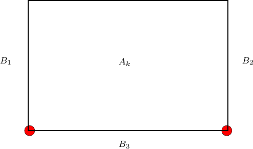 \n",
"\n",
"In the sequence, we present the *stencils* for each of these *pdes*.\n",
"\n",
"So, for the A1 case we have the following *pdes* and *stencils*:"
]
},
{
"cell_type": "code",
"execution_count": 37,
"metadata": {},
"outputs": [],
"source": [
"if(habctype == 1):\n",
"\n",
" # Region B_{1}\n",
" aux1 = ((-vel[x, z]*dt+hx)*u2[x, z] + (vel[x, z]*dt+hx)*u2[x+1, z] + (vel[x, z]*dt-hx)*u3[x+1, z])/(vel[x, z]*dt+hx)\n",
" pde1 = (1-weightsx[x, z])*u3[x, z] + weightsx[x, z]*aux1\n",
" stencil1 = Eq(u.forward, pde1, subdomain=grid.subdomains['d1'])\n",
"\n",
" # Region B_{3}\n",
" aux2 = ((-vel[x, z]*dt+hx)*u2[x, z] + (vel[x, z]*dt+hx)*u2[x-1, z] + (vel[x, z]*dt-hx)*u3[x-1, z])/(vel[x, z]*dt+hx)\n",
" pde2 = (1-weightsx[x, z])*u3[x, z] + weightsx[x, z]*aux2\n",
" stencil2 = Eq(u.forward, pde2, subdomain=grid.subdomains['d2'])\n",
"\n",
" # Region B_{2}\n",
" aux3 = ((-vel[x, z]*dt+hz)*u2[x, z] + (vel[x, z]*dt+hz)*u2[x, z-1] + (vel[x, z]*dt-hz)*u3[x, z-1])/(vel[x, z]*dt+hz)\n",
" pde3 = (1-weightsz[x, z])*u3[x, z] + weightsz[x, z]*aux3\n",
" stencil3 = Eq(u.forward, pde3, subdomain=grid.subdomains['d3'])"
]
},
{
"cell_type": "markdown",
"metadata": {},
"source": [
"For the A2 case we have the following *pdes* and *stencils*:"
]
},
{
"cell_type": "code",
"execution_count": 38,
"metadata": {},
"outputs": [],
"source": [
"if(habctype == 2):\n",
"\n",
" # Region B_{1}\n",
" cte11 = (1/(2*dt**2)) + (1/(2*dt*hx))*vel[x, z]\n",
" cte21 = -(1/(2*dt**2)) + (1/(2*dt*hx))*vel[x, z] - (1/(2*hz**2))*vel[x, z]*vel[x, z]\n",
" cte31 = -(1/(2*dt**2)) - (1/(2*dt*hx))*vel[x, z]\n",
" cte41 = (1/(dt**2))\n",
" cte51 = (1/(4*hz**2))*vel[x, z]**2\n",
"\n",
" aux1 = (\n",
" cte21*(u3[x+1, z] + u1[x, z])\n",
" + cte31*u1[x+1, z] + cte41*(u2[x, z]+u2[x+1, z])\n",
" + cte51*(u3[x+1, z+1] + u3[x+1, z-1] + u1[x, z+1] + u1[x, z-1])\n",
" )/cte11\n",
" pde1 = (1-weightsx[x, z])*u3[x, z] + weightsx[x, z]*aux1\n",
" stencil1 = Eq(u.forward, pde1, subdomain=grid.subdomains['d1'])\n",
"\n",
" # Region B_{3}\n",
" cte12 = (1/(2*dt**2)) + (1/(2*dt*hx))*vel[x, z]\n",
" cte22 = -(1/(2*dt**2)) + (1/(2*dt*hx))*vel[x, z] - (1/(2*hz**2))*vel[x, z]**2\n",
" cte32 = -(1/(2*dt**2)) - (1/(2*dt*hx))*vel[x, z]\n",
" cte42 = (1/(dt**2))\n",
" cte52 = (1/(4*hz**2))*vel[x, z]*vel[x, z]\n",
"\n",
" aux2 = (\n",
" cte22*(u3[x-1, z] + u1[x, z])\n",
" + cte32*u1[x-1, z] + cte42*(u2[x, z]+u2[x-1, z])\n",
" + cte52*(u3[x-1, z+1] + u3[x-1, z-1] + u1[x, z+1] + u1[x, z-1])\n",
" )/cte12\n",
" pde2 = (1-weightsx[x, z])*u3[x, z] + weightsx[x, z]*aux2\n",
" stencil2 = Eq(u.forward, pde2, subdomain=grid.subdomains['d2'])\n",
"\n",
" # Region B_{2}\n",
" cte13 = (1/(2*dt**2)) + (1/(2*dt*hz))*vel[x, z]\n",
" cte23 = -(1/(2*dt**2)) + (1/(2*dt*hz))*vel[x, z] - (1/(2*hx**2))*vel[x, z]**2\n",
" cte33 = -(1/(2*dt**2)) - (1/(2*dt*hz))*vel[x, z]\n",
" cte43 = (1/(dt**2))\n",
" cte53 = (1/(4*hx**2))*vel[x, z]*vel[x, z]\n",
"\n",
" aux3 = (\n",
" cte23*(u3[x, z-1] + u1[x, z])\n",
" + cte33*u1[x, z-1] + cte43*(u2[x, z]+u2[x, z-1])\n",
" + cte53*(u3[x+1, z-1] + u3[x-1, z-1] + u1[x+1, z] + u1[x-1, z])\n",
" )/cte13\n",
" pde3 = (1-weightsz[x, z])*u3[x, z] + weightsz[x, z]*aux3\n",
" stencil3 = Eq(u.forward, pde3, subdomain=grid.subdomains['d3'])\n",
"\n",
" # Red point right side\n",
" stencil4 = [\n",
" Eq(\n",
" u[t+1, nptx-1-k, nptz-1-k],\n",
" (1-weightsz[nptx-1-k, nptz-1-k])*u3[nptx-1-k, nptz-1-k]\n",
" + weightsz[nptx-1-k, nptz-1-k]*(((-(1/(4*hx))\n",
" + (1/(4*hz)) - (np.sqrt(2))/(4*vel[nptx-1-k, nptz-1-k]*dt))*u3[nptx-1-k, nptz-2-k]\n",
" + ((1/(4*hx)) - (1/(4*hz)) - (np.sqrt(2))/(4*vel[nptx-1-k, nptz-1-k]*dt))*u3[nptx-2-k, nptz-1-k]\n",
" + ((1/(4*hx)) + (1/(4*hz)) - (np.sqrt(2))/(4*vel[nptx-1-k, nptz-1-k]*dt))*u3[nptx-2-k, nptz-2-k]\n",
" + (-(1/(4*hx)) - (1/(4*hz)) + (np.sqrt(2))/(4*vel[nptx-1-k, nptz-1-k]*dt))*u2[nptx-1-k, nptz-1-k]\n",
" + (-(1/(4*hx)) + (1/(4*hz)) + (np.sqrt(2))/(4*vel[nptx-1-k, nptz-1-k]*dt))*u2[nptx-1-k, nptz-2-k]\n",
" + ((1/(4*hx)) - (1/(4*hz)) + (np.sqrt(2))/(4*vel[nptx-1-k, nptz-1-k]*dt))*u2[nptx-2-k, nptz-1-k]\n",
" + ((1/(4*hx)) + (1/(4*hz)) + (np.sqrt(2))/(4*vel[nptx-1-k, nptz-1-k]*dt))*u2[nptx-2-k, nptz-2-k])\n",
" / ((1/(4*hx)) + (1/(4*hz)) + (np.sqrt(2))/(4*vel[nptx-1-k, nptz-1-k]*dt)))) for k in range(0, npmlz)\n",
" ]\n",
"\n",
" # Red point left side\n",
" stencil5 = [\n",
" Eq(\n",
" u[t+1, k, nptz-1-k],\n",
" (1-weightsx[k, nptz-1-k])*u3[k, nptz-1-k]\n",
" + weightsx[k, nptz-1-k]*(((-(1/(4*hx))\n",
" + (1/(4*hz)) - (np.sqrt(2))/(4*vel[k, nptz-1-k]*dt))*u3[k, nptz-2-k]\n",
" + ((1/(4*hx)) - (1/(4*hz)) - (np.sqrt(2))/(4*vel[k, nptz-1-k]*dt))*u3[k+1, nptz-1-k]\n",
" + ((1/(4*hx)) + (1/(4*hz)) - (np.sqrt(2))/(4*vel[k, nptz-1-k]*dt))*u3[k+1, nptz-2-k]\n",
" + (-(1/(4*hx)) - (1/(4*hz)) + (np.sqrt(2))/(4*vel[k, nptz-1-k]*dt))*u2[k, nptz-1-k]\n",
" + (-(1/(4*hx)) + (1/(4*hz)) + (np.sqrt(2))/(4*vel[k, nptz-1-k]*dt))*u2[k, nptz-2-k]\n",
" + ((1/(4*hx)) - (1/(4*hz)) + (np.sqrt(2))/(4*vel[k, nptz-1-k]*dt))*u2[k+1, nptz-1-k]\n",
" + ((1/(4*hx)) + (1/(4*hz)) + (np.sqrt(2))/(4*vel[k, nptz-1-k]*dt))*u2[k+1, nptz-2-k])\n",
" / ((1/(4*hx)) + (1/(4*hz)) + (np.sqrt(2))/(4*vel[k, nptz-1-k]*dt)))\n",
" ) for k in range(0, npmlx)\n",
" ]"
]
},
{
"cell_type": "markdown",
"metadata": {},
"source": [
"For the Higdon case we have the following *pdes* and *stencils*:"
]
},
{
"cell_type": "code",
"execution_count": 39,
"metadata": {},
"outputs": [],
"source": [
"if(habctype == 3):\n",
"\n",
" alpha1 = 0.0\n",
" alpha2 = np.pi/4\n",
" a1 = 0.5\n",
" b1 = 0.5\n",
" a2 = 0.5\n",
" b2 = 0.5\n",
"\n",
" # Region B_{1}\n",
" gama111 = np.cos(alpha1)*(1-a1)*(1/dt)\n",
" gama121 = np.cos(alpha1)*(a1)*(1/dt)\n",
" gama131 = np.cos(alpha1)*(1-b1)*(1/hx)*vel[x, z]\n",
" gama141 = np.cos(alpha1)*(b1)*(1/hx)*vel[x, z]\n",
"\n",
" gama211 = np.cos(alpha2)*(1-a2)*(1/dt)\n",
" gama221 = np.cos(alpha2)*(a2)*(1/dt)\n",
" gama231 = np.cos(alpha2)*(1-b2)*(1/hx)*vel[x, z]\n",
" gama241 = np.cos(alpha2)*(b2)*(1/hx)*vel[x, z]\n",
"\n",
" c111 = gama111 + gama131\n",
" c121 = -gama111 + gama141\n",
" c131 = gama121 - gama131\n",
" c141 = -gama121 - gama141\n",
"\n",
" c211 = gama211 + gama231\n",
" c221 = -gama211 + gama241\n",
" c231 = gama221 - gama231\n",
" c241 = -gama221 - gama241\n",
"\n",
" aux1 = (\n",
" u2[x, z]*(-c111*c221-c121*c211)\n",
" + u3[x+1, z]*(-c111*c231-c131*c211)\n",
" + u2[x+1, z]*(-c111*c241-c121*c231-c141*c211-c131*c221)\n",
" + u1[x, z]*(-c121*c221)\n",
" + u1[x+1, z]*(-c121*c241-c141*c221)\n",
" + u3[x+2, z]*(-c131*c231)\n",
" + u2[x+2, z]*(-c131*c241-c141*c231)\n",
" + u1[x+2, z]*(-c141*c241)\n",
" )/(c111*c211)\n",
" pde1 = (1-weightsx[x, z])*u3[x, z] + weightsx[x, z]*aux1\n",
" stencil1 = Eq(u.forward, pde1, subdomain=grid.subdomains['d1'])\n",
"\n",
" # Region B_{3}\n",
" gama112 = np.cos(alpha1)*(1-a1)*(1/dt)\n",
" gama122 = np.cos(alpha1)*(a1)*(1/dt)\n",
" gama132 = np.cos(alpha1)*(1-b1)*(1/hx)*vel[x, z]\n",
" gama142 = np.cos(alpha1)*(b1)*(1/hx)*vel[x, z]\n",
"\n",
" gama212 = np.cos(alpha2)*(1-a2)*(1/dt)\n",
" gama222 = np.cos(alpha2)*(a2)*(1/dt)\n",
" gama232 = np.cos(alpha2)*(1-b2)*(1/hx)*vel[x, z]\n",
" gama242 = np.cos(alpha2)*(b2)*(1/hx)*vel[x, z]\n",
"\n",
" c112 = gama112 + gama132\n",
" c122 = -gama112 + gama142\n",
" c132 = gama122 - gama132\n",
" c142 = -gama122 - gama142\n",
"\n",
" c212 = gama212 + gama232\n",
" c222 = -gama212 + gama242\n",
" c232 = gama222 - gama232\n",
" c242 = -gama222 - gama242\n",
"\n",
" aux2 = (\n",
" u2[x, z]*(-c112*c222-c122*c212)\n",
" + u3[x-1, z]*(-c112*c232-c132*c212)\n",
" + u2[x-1, z]*(-c112*c242-c122*c232-c142*c212-c132*c222)\n",
" + u1[x, z]*(-c122*c222)\n",
" + u1[x-1, z]*(-c122*c242-c142*c222)\n",
" + u3[x-2, z]*(-c132*c232)\n",
" + u2[x-2, z]*(-c132*c242-c142*c232)\n",
" + u1[x-2, z]*(-c142*c242)\n",
" )/(c112*c212)\n",
" pde2 = (1-weightsx[x, z])*u3[x, z] + weightsx[x, z]*aux2\n",
" stencil2 = Eq(u.forward, pde2, subdomain=grid.subdomains['d2'])\n",
"\n",
" # Region B_{2}\n",
" gama113 = np.cos(alpha1)*(1-a1)*(1/dt)\n",
" gama123 = np.cos(alpha1)*(a1)*(1/dt)\n",
" gama133 = np.cos(alpha1)*(1-b1)*(1/hz)*vel[x, z]\n",
" gama143 = np.cos(alpha1)*(b1)*(1/hz)*vel[x, z]\n",
"\n",
" gama213 = np.cos(alpha2)*(1-a2)*(1/dt)\n",
" gama223 = np.cos(alpha2)*(a2)*(1/dt)\n",
" gama233 = np.cos(alpha2)*(1-b2)*(1/hz)*vel[x, z]\n",
" gama243 = np.cos(alpha2)*(b2)*(1/hz)*vel[x, z]\n",
"\n",
" c113 = gama113 + gama133\n",
" c123 = -gama113 + gama143\n",
" c133 = gama123 - gama133\n",
" c143 = -gama123 - gama143\n",
"\n",
" c213 = gama213 + gama233\n",
" c223 = -gama213 + gama243\n",
" c233 = gama223 - gama233\n",
" c243 = -gama223 - gama243\n",
"\n",
" aux3 = (\n",
" u2[x, z]*(-c113*c223-c123*c213)\n",
" + u3[x, z-1]*(-c113*c233-c133*c213)\n",
" + u2[x, z-1]*(-c113*c243-c123*c233-c143*c213-c133*c223)\n",
" + u1[x, z]*(-c123*c223)\n",
" + u1[x, z-1]*(-c123*c243-c143*c223)\n",
" + u3[x, z-2]*(-c133*c233)\n",
" + u2[x, z-2]*(-c133*c243-c143*c233)\n",
" + u1[x, z-2]*(-c143*c243)\n",
" )/(c113*c213)\n",
" pde3 = (1-weightsz[x, z])*u3[x, z] + weightsz[x, z]*aux3\n",
" stencil3 = Eq(u.forward, pde3, subdomain=grid.subdomains['d3'])"
]
},
{
"cell_type": "markdown",
"metadata": {},
"source": [
"The surface boundary conditions of the problem are the same as in the notebook Introduction to Acoustic Problem. They are placed in the term *bc* and have the following form:"
]
},
{
"cell_type": "code",
"execution_count": 40,
"metadata": {},
"outputs": [],
"source": [
"bc = [Eq(u[t+1, x, 0], u[t+1, x, 1])]"
]
},
{
"cell_type": "markdown",
"metadata": {},
"source": [
"We will then define the operator (*op*) that will join the acoustic equation, source term, boundary conditions and receivers.\n",
"\n",
"- 1. The acoustic wave equation in the *d0* region: *[stencil01];*\n",
"- 2. Source term: *src_term;*\n",
"- 3. Updating solutions over time: *[stencil01,stencil02];*\n",
"- 4. The acoustic wave equation in the *d1*, *d2* e *d3* regions: *[stencil1,stencil2,stencil3];*\n",
"- 5. The equation for red points for A2 method: *[stencil5,stencil4];*\n",
"- 6. Boundary Conditions: *bc;*\n",
"- 7. Receivers: *rec_term;*\n",
"\n",
"We then define two types of *op*:\n",
"\n",
"- The first *op* is for the cases A1 and Higdon;\n",
"- The second *op* is for the case A2;\n",
"\n",
"The *ops* are constructed by the following commands:"
]
},
{
"cell_type": "code",
"execution_count": 41,
"metadata": {},
"outputs": [],
"source": [
"# NBVAL_IGNORE_OUTPUT\n",
"\n",
"if(habctype != 2):\n",
" op = Operator(\n",
" [stencil0]\n",
" + src_term\n",
" + [stencil01, stencil3, stencil02, stencil2, stencil1]\n",
" + bc\n",
" + rec_term,\n",
" subs=grid.spacing_map\n",
" )\n",
"else:\n",
" op = Operator(\n",
" [stencil0]\n",
" + src_term\n",
" + [stencil01, stencil3, stencil02, stencil2, stencil1, stencil02, stencil4, stencil5]\n",
" + bc\n",
" + rec_term,\n",
" subs=grid.spacing_map\n",
" )"
]
},
{
"cell_type": "markdown",
"metadata": {},
"source": [
"Initially:"
]
},
{
"cell_type": "code",
"execution_count": 42,
"metadata": {},
"outputs": [],
"source": [
"u.data[:] = 0.\n",
"u1.data[:] = 0.\n",
"u2.data[:] = 0.\n",
"u3.data[:] = 0."
]
},
{
"cell_type": "markdown",
"metadata": {},
"source": [
"We assign to *op* the number of time steps it must execute and the size of the time step in the local variables *time* and *dt*, respectively."
]
},
{
"cell_type": "code",
"execution_count": 43,
"metadata": {},
"outputs": [
{
"name": "stderr",
"output_type": "stream",
"text": [
"Operator `Kernel` ran in 0.04 s\n"
]
},
{
"data": {
"text/plain": [
"PerformanceSummary([(PerfKey(name='section0', rank=None),\n",
" PerfEntry(time=0.006794999999999992, gflopss=0.0, gpointss=0.0, oi=0.0, ops=0, itershapes=[])),\n",
" (PerfKey(name='section1', rank=None),\n",
" PerfEntry(time=0.0017370000000000076, gflopss=0.0, gpointss=0.0, oi=0.0, ops=0, itershapes=[])),\n",
" (PerfKey(name='section2', rank=None),\n",
" PerfEntry(time=0.007607999999999926, gflopss=0.0, gpointss=0.0, oi=0.0, ops=0, itershapes=[])),\n",
" (PerfKey(name='section3', rank=None),\n",
" PerfEntry(time=0.004895000000000037, gflopss=0.0, gpointss=0.0, oi=0.0, ops=0, itershapes=[])),\n",
" (PerfKey(name='section4', rank=None),\n",
" PerfEntry(time=0.0027840000000000343, gflopss=0.0, gpointss=0.0, oi=0.0, ops=0, itershapes=[])),\n",
" (PerfKey(name='section5', rank=None),\n",
" PerfEntry(time=0.006082000000000047, gflopss=0.0, gpointss=0.0, oi=0.0, ops=0, itershapes=[])),\n",
" (PerfKey(name='section6', rank=None),\n",
" PerfEntry(time=0.0014940000000000192, gflopss=0.0, gpointss=0.0, oi=0.0, ops=0, itershapes=[])),\n",
" (PerfKey(name='section7', rank=None),\n",
" PerfEntry(time=0.0024470000000000134, gflopss=0.0, gpointss=0.0, oi=0.0, ops=0, itershapes=[]))])"
]
},
"execution_count": 43,
"metadata": {},
"output_type": "execute_result"
}
],
"source": [
"# NBVAL_IGNORE_OUTPUT\n",
"\n",
"op(time=nt, dt=dt0)"
]
},
{
"cell_type": "markdown",
"metadata": {},
"source": [
"We view the result of the displacement field at the end time using the *graph2d* routine given by:"
]
},
{
"cell_type": "code",
"execution_count": 44,
"metadata": {},
"outputs": [],
"source": [
"def graph2d(U, i):\n",
" plot.figure()\n",
" plot.figure(figsize=(16, 8))\n",
" fscale = 1/10**(3)\n",
" x0pml = x0 + npmlx*hxv\n",
" x1pml = x1 - npmlx*hxv\n",
" z0pml = z0\n",
" z1pml = z1 - npmlz*hzv\n",
" scale = np.amax(U[npmlx:-npmlx, 0:-npmlz])/10.\n",
" extent = [fscale*x0pml, fscale*x1pml, fscale*z1pml, fscale*z0pml]\n",
" fig = plot.imshow(np.transpose(U[npmlx:-npmlx, 0:-npmlz]), vmin=-scale, vmax=scale, cmap=cm.seismic, extent=extent)\n",
" plot.gca().xaxis.set_major_formatter(mticker.FormatStrFormatter('%.1f km'))\n",
" plot.gca().yaxis.set_major_formatter(mticker.FormatStrFormatter('%.1f km'))\n",
" plot.axis('equal')\n",
" if(i == 1):\n",
" plot.title('Map - Acoustic Problem with Devito - HABC A1')\n",
" if(i == 2):\n",
" plot.title('Map - Acoustic Problem with Devito - HABC A2')\n",
" if(i == 3):\n",
" plot.title('Map - Acoustic Problem with Devito - HABC Higdon')\n",
" plot.grid()\n",
" ax = plot.gca()\n",
" divider = make_axes_locatable(ax)\n",
" cax = divider.append_axes(\"right\", size=\"5%\", pad=0.05)\n",
" cbar = plot.colorbar(fig, cax=cax, format='%.2e')\n",
" cbar.set_label('Displacement [km]')\n",
" plot.draw()\n",
" plot.show()"
]
},
{
"cell_type": "code",
"execution_count": 45,
"metadata": {},
"outputs": [
{
"data": {
"text/plain": [
""
]
},
"metadata": {},
"output_type": "display_data"
},
{
"data": {
"image/png": "iVBORw0KGgoAAAANSUhEUgAAA4gAAAK2CAYAAAAMt7KnAAAAOnRFWHRTb2Z0d2FyZQBNYXRwbG90bGliIHZlcnNpb24zLjEwLjMsIGh0dHBzOi8vbWF0cGxvdGxpYi5vcmcvZiW1igAAAAlwSFlzAAAPYQAAD2EBqD+naQABAABJREFUeJzs3Xd4FFXbBvB70xuEEEgCpNFRQCAUUUBpgqBUBQQpUREUEMFGeUWCImDhExALKlUUpUZAmiAtoEiJFKUECBA6JKSQRsp+f4Rds8l5NjubTSHcv+vKJT4zc+bszOzsnj1nnqPT6/V6EBERERER0X3PrqQrQERERERERKUDG4hEREREREQEgA1EIiIiIiIiuosNRCIiIiIiIgLABiIRERERERHdxQYiERERERERAWADkYiIiIiIiO5iA5GIiIiIiIgAsIFIREREREREd7GBqLBo0SLodDrjX/fu3S3arlevXibbLVq0qGgreg/KyMiAj4+P8RjNmzevpKtUJpTUNZf3vWL4s7OzQ4UKFRASEoI33ngDp0+fLtZ6matnSZZxP7PV8QsNDYVOp0Pbtm1tUzGFc+fOKa9rR0dHeHt7o0aNGnjyySfxv//9D7t37y6yethScRy30qZt27bQ6XQIDg62aH3DMbL0GrX28ywsLEx5fRmuMV9fX3Ts2BFff/010tPTLSoTAPbs2YM33ngDISEh8PX1hZOTEypUqIAHH3wQgwcPxqpVqzSVl5vWY5P7NZ47dy7fcsO5CQ0Ntao+thIcHAydToewsLASrQdRacMGogU2bdqEGzdumF0nNjYWv/76azHV6N61ceNGk2O5ZMmSEqxN6Wb4gLX0y01potfrkZCQgMjISHz22Wdo0KABFi5cWNLVolLsXvhhLTMzE3FxcYiOjsbmzZsxbdo0PPbYY3jwwQexcePGkq6e1Xbs2GH2yzypFcXnWWZmJq5fv45t27bh1VdfRdOmTXH58mWz25w/fx6dO3dG69at8dlnnyEyMhLXr19HRkYGEhIScPz4cXz//fd49tlnUaNGDfz888+FricRlW1sIBagfPnyyMjIwLJly8yut2zZMmRkZKB8+fLFVLN70+LFi03+f+/evYiKiiqh2pAtbdiwAUlJSUhKSkJCQgJOnjyJDz/8EM7OzkhPT8fLL7+MvXv3lnQ1iTSZMGGC8bpOTEzEpUuX8Pfff+O7775Dt27doNPpcPz4cXTt2hWTJk0q6epSMbLF59k///xjvL6SkpJw8eJF7NixA7169TIu79Onj7h9ZGQkHn74YWzZsgUA0KlTJyxZsgQnTpxAbGwszp07h99//x1vvfUWvL29cfnyZXz11VcaXykR3W/YQCzAs88+C6DgXwYNy83dyO93cXFxWL9+PQCge/fuxqEq7EUsPL1eD71eX6LDdVxdXeHh4QEPDw+UL18ederUwcSJE43DrrKysjBt2rQSqx+VrNDQUON1ei9xcnIyXtflypVD1apV0ahRI7z00ktYu3Yt9u/fb+zlnzp1Kr777ruSrbBg0aJF0Ov12LFjR0lXpUyw1eeZm5ub8fry8PBAtWrV8Pjjj2P16tXGRuLevXvx559/5ts2NjYWPXr0wLVr1+Ds7Izly5dj8+bNGDRoEOrWrYuKFSsiKCgI7dq1wyeffIKzZ8/ijTfeKBXD5Hfs2AG9Xl+qRwwQ3c/YQCzAwIEDYWdnh4MHD+L48ePKdU6cOIH9+/fDzs4OAwcOLOYa3juWLVuGO3fuAAAmT56M1q1bAwC+//77e+5LI1lu8ODBqF69OgBg+/btyMrKKuEaEdlO06ZNsXXrVuPokXfeeQdJSUklXCsqasXxefbyyy8b/71///58y8eNG4eYmBgAwLffflvgD9Tly5fHzJkzMXfuXJvUj4jKLjYQCxAQEGB8qF/6ZdAQb9euHfz9/c2Wp9fr8ddff+Hdd9/Fo48+Cm9vbzg6OsLLywvNmzfH5MmTERsbK26fN9HDhQsXMHLkSNSoUQMuLi7w8fHBM888gz/++MOKV1u0DMNxHnzwQYSEhGDw4MEAcp6fsPRX7aNHj2LEiBGoX78+PD094ebmhtq1a6NHjx5YvHix+MUsNjYWkyZNQkhICCpUqAAXFxcEBwdj8ODB+Ouvv8T9WZpYo6AEEOfPn8fYsWPRsGFDeHh4wMnJCVWrVkXjxo0xbNgwrFmzxriu4XmgKVOmGLfNm8gg73OJljy/lZ6ejq+//hpPPvkkqlSpAmdnZ/j6+qJZs2Z45513cOjQIbOv0Vo6nQ4PPvggACAlJQVxcXEATBOB7NixA2lpafj444/RvHlzeHl5KV/PhQsXMHbsWNSvXx/lypUznv9XXnkFJ06csLhORfm+OXPmDMaMGYMGDRqgfPnycHV1Ra1atTBs2DCcPHlS3C5v0obt27eje/fu8PPzg5ubG+rXr4+PP/7YJMlEQkICPvzwQ+N15eXlha5du2Lfvn1W1d1wvTs7OyMlJSXf8t9++814zpo1a6YsY+rUqdDpdKhataqy7LzvJcPrNnjhhRfyXe/mrusjR45g4MCB8Pf3h7OzM6pVq4bQ0FCcOXNGwysvnJo1a2LcuHEAgFu3bpl93jYhIQHTp0/Ho48+ikqVKsHZ2RlVq1ZF7969jcMEc8vOzkZAQAB0Op3xnmnO4MGDjcc/948x0j1Kp9OhXbt2xv+vXr16vuOvei7x33//xfDhw1G7dm24ubmhXLlyqF+/Pt58801cvHixwHre62zxeVaQoKAg47/zvh+vXLmC77//HgDQunVrDBo0yOJy69evb5P6FYYlSWpiYmLw6quvIigoyPg+6dOnj/H+ZkkZJ06cwODBg1GtWjU4OzsjICAAQ4YMwbFjxyyuq7WfO3nveTdv3sTbb7+N2rVrw8XFBd7e3ujSpQu2b99ucV2Iio2e8lm4cKEegB6APioqSr9o0SI9AH1AQIA+KyvLZN3s7Gx9YGCgHoB+8eLF+qioKOO2CxcuzFd2eHi4cbn05+fnp4+MjCywbgcOHNBXrFhRWYadnZ1+zpw5RXB0rPPvv/8a6zZ9+nS9Xq/Xx8fH611cXPQA9KGhoWa3z8rK0r/zzjt6nU5n9tipjvnOnTv1Xl5eZrcbP368cr+5j7c5Q4YM0QPQP/744/mW7dixQ+/u7m52/+7u7sb1t2/fXuA1EhQUZLIPc69fr9frjxw5oq9Ro4amMi2R+/hs375dXK9bt27G9a5du6bX6/X66OhoY2zVqlX6hx56yOz5XLFihfF6Uf3Z29vr586dW2A9rX3fWHItzJ49W+/o6CjW0cHBQb9gwQLlto8//rgegH7IkCH6GTNmiNd6165d9RkZGfpz587p69Wrp1zHyclJv3XrVrGeknPnzhnL2LJlS77lEyZMMDlWt27dyrdO+/bt9QD0AwYMMIlLx8/wui19X+d+r/300096Z2dn5TZeXl76I0eOaD4Ger3ptTl58mSLtrl69apxm6eeekq5zs6dO/WVKlUy+1qHDRumz8zMNNlu3LhxegB6Dw8PfXJysliH5ORkvYeHhx6A/q233jJZJt2jCjr2APTR0dEm28yaNUtvb28vru/q6qpfvXq1RcetKBmuLUvvbYZjVND9vrCfZ5MnTxaPbW4bN240rrd06VKTZV9//bVx2eLFiy16fYVh6bExKOg15r7fqUREROjLly8v3kfnz59fYBnh4eHi/cHV1VW/fv16fVBQkNn3ua0+d/755x99tWrVlGXodLpiOYdEWrAH0QLPPPMM3N3dERMTk++Xnu3bt+PChQtwd3fHM888U2BZDg4O6N69O+bNm4eIiAicOXMGN2/exLFjxzBv3jzUqVMHV69eRe/evZGWlma2rD59+sDBwQHfffcdYmJicPXqVfz888+oXr06srOzMXr0aGzdurVQr91WDL+25h6G6+npiR49egAAVq5cieTkZHH7t99+Gx9//DH0ej2aNm2Kn3/+GRcuXEBcXBz+/fdfzJ8/Hx07dszXO3HmzBk89dRTuHXrFjw9PTF79mxER0fj+vXr2LRpE5o3bw4AmDFjBmbOnGnz152dnY3BgwcjOTkZPj4+mDdvHk6ePIm4uDhcvnwZu3fvxtSpU1G3bl3jNm3atEFSUhImTJgAAAgMDDRJYpCUlIR///3X4jqcO3cObdu2xdmzZ+Hi4oJ33nkHBw4cwM2bN3H58mVs27YNb731Fnx8fGz++g0M9TX8aprX66+/jlOnTmHKlCk4fvw4bt68ib/++gstWrQAkPMMznPPPYe0tDRUrVoVCxcuxMWLF3H16lWsXLkSderUQVZWFkaNGoXVq1ebrUtRvW++/vprvP7668jIyEC3bt2wadMmXL58GTdv3sSOHTvQpUsXZGZmYujQodi2bZtYzs6dOzFhwgRjj2ZsbCyOHz+OF198EUBOMqAFCxagT58+uHXrFubNm4fz58/jxo0bWLVqFfz8/HDnzh289NJLyMzM1PQagoKCTIYD52WIOTo6Ijs7Gzt37jRZnp6ebkxElLtXypyNGzea9Px//fXX+a531dD906dPY8iQIcYEHdevX0dMTAxmzZoFZ2dn3Lp1C8OHD7fshduAr68vatasCQDKnui///4bnTt3xs2bN9GwYUMsXboU0dHRiIuLw+HDhzFmzBjodDp88803eP/99022NfQO3b59G+Hh4WId1qxZg9u3b5tsU5CkpCRs2LDB+P95k6YkJSWZ9GQtX74cY8aMQVZWFurWrYtVq1bh6tWruHjxIhYsWIAqVaogNTUVffv2tbonu7Qr7OeZpb799lsAOe+3xx9/3GRZ7ulVHnvssULvqzS5du0aunfvjsTERJQrVw6fffaZ8XN7y5YtCAkJwYgRI8yOEjhx4gT69euH9PR0VKpUCd98843J/d7Pzw+DBg1CQkKCWIYtP3e6desGR0dHLFmyBDExMbhx4wbWrFmDgIAA6PV6jBw50uzoMaJiV9It1NIobw+iXq/XDxw4UPlLleFXtUGDBun1en2BPYgFSUpK0tesWVMPQNnTkLtubm5u+n///TffOpcuXdL7+vrqAejr16+vuQ62lpWVZfzlrH379ibLNmzYYHw9S5YsUW6/b98+4zo9evTQ37lzR9xXRkaGyf/37NnT2KOyf//+fOunpKToW7RooQegd3Fx0d+4ccNkeWF7EI8cOWLc/pdffjFbRl6GX2At+fXb3DXXpUsX4zHYvXu3WEbeY2cJS3oQly1bZlynU6dOxnjuXhoA+l9//VXcT5MmTYy9Qqpfo2/evKmvXr26HoC+SpUq+a4RW7xvzF0LV65cMf7KPHHiROVryM7O1vfr108PQN+wYcN8y3P3pL388svKMlq1amX8Bb1cuXL6U6dO5Vtn8+bNxnI2b96sLMecF198UQ9A//DDD5vEExMT9Q4ODno7Ozv9yy+/rAegHz16tMk6O3bsMO779OnTJssKei9Zet/M3ZPx5JNPKq/bmTNnGtc5fvy4Ba/alDU9iHq9Xv/kk08at0tPTzdZ1rhxYz0Afbt27fRpaWnK7b/88kvje/Xy5csmywzvgSeffFLcf+fOnfUA9A899FC+ZeZGOeQetWCuRys9Pd34HqlZs6Y+NjY23zpnzpzRV6hQQQ9A37RpU7Gs4mB4TwUGBuqTkpIK/Hv++ecLvN8X9vNMrzftXfvnn39M6nDp0iX9rl279M8++6xxHdUIl0cffdT4uVUccr/vLDmWuUcbaO1BHDlypB7IGaWwc+fOfMtTUlKM7wepDMOoFRcXF/2xY8fyLc99v5fe57b83KlWrZpx9ExuBw8eNK7z1Vdf5VtOVFLYg2ghw/MFq1atMj4LkJKSglWrVpksLywPDw/07t0bQM7zPuaMHDkSDzzwQL541apV8b///Q9Azq/BJf0r7tatW3Hp0iUA+Y9Tp06d4OfnByB/ynCDWbNmAcg5NgsXLoSjo6O4LwcHB+O/r1+/jrVr1wLIedhf9cyUq6sr5syZAwBIS0szPtNhK7l7cPI+k1UcTp06ZZyf7a233jImUlDJfewKS6/X48qVK/j8888xdOhQADnPOhme08rrySefRNeuXZXLDh48iMjISADAxIkTlfNCent7Y/r06QByns0xZBdUKYr3zddff420tDQEBQUZnx3NS6fT4aOPPgKQ8yztkSNHlOu5ubnh448/Vi577rnnAORcV6NHj0bt2rXzrfPEE08Ye2mtee8bev4OHjxo0rO3e/duZGZmolGjRsbREr///rvJtoYexoCAAGNvWlGaPXu28rrN/UySKrlHUalQoYLx37du3TL+e8eOHfj777+Nk6k7Ozsrt3/llVdQo0YN3LlzBytWrDBZZugR/O2333Dt2rV82169etXY822rz6O81q1bZ9z3jBkzULFixXzr1KhRA+PHjwdg+t4tSRcuXEC5cuUK/Pvhhx8KLKuwn2d5GZ5rM/xVq1YNjz32GFauXIlGjRph4cKFxntbboZnuXNfc8XFkmOpqrMlMjMzsXTpUgA5WeRVvaOurq6YMWOGWMb169eN81K/+uqrymcuc9/vVWz9ufPee+8pR+mEhITgoYceAlC89yqigrCBaKEOHTqgWrVquH37tnEowerVq3H79m1Uq1YN7du3t7iszMxMLF68GN27d0dgYCDc3NxMEgJ88sknAGA2oQUAY0NSJfdw1z179lhct6Jg+KB0c3PLNwzX3t4eAwYMAJDz5dKQkS03w3C87t27w8vLy+L97t27F9nZ2QCAvn37ius9/PDDxiFUuYft2ELdunXh4uICAHjttddw+PBhm5ZfkNxDJYt6Cox27doZr2E7OztUrVoVo0ePRnJyMuzt7fHZZ5+J75OnnnpKLDf3OTF3Hnv27AknJ6d82+RVFO8bw3Fu37490tLScPv2beWft7c3KlWqBED+MtCyZUvxS1/uRlfnzp2V6+h0OuN6V65csfg1GBiSmGRmZpocR0Pjr3379mjdujUcHR3xzz//mEwUbljH0uGlhVGjRg3UqVNHuaxixYqoXLkygJyGU3HR58pemXu4u+H6qFmzJqpUqSJeH8nJyWjUqBGA/NdH//79YW9vj6ysLOW8vMuWLUNWVpbJPdXWDNeDs7MzunfvLq7Xr1+/fNuUFYX9PNPixIkT+PXXX3HhwoVClXMvOXbsmHHYp2HIrkrHjh3h7u6uXJb7s9/S+31etv7c6dKli7jM8IhJcd6riArCBqKF7OzsjDd+Q9ZSw3+ff/552NlZdiivX7+Ohx9+GKGhoVi3bh1iYmKQmpqqXNfc2HgAyl4Qg6pVq8LT0xMAlBnoJHq9XvzyospqWJDExERjhs5evXrBw8Mj3zqGX2Gzs7ONvxwaJCUl4fr16wCAxo0ba9r3+fPnjf82ZNGUGH5h1HKsLOHm5oapU6cCAP788080btwYNWrUwAsvvIAFCxYU+gtEQQzPaBiyrhUne3t71KxZEy+99BIOHjyI119/XVy3Ro0a4jLDeXR3d0dgYKC4nrOzM2rVqgXA/HksiveNIZPdwoULC/xl/ebNmwBg0rDKWweJq6urpvWke4s5/v7+xuOY+znE3I0/d3d3tGjRAnq93hhPTU01ztVWHA3Egnrk3dzcAOTP/liUct+zc/euGa6P06dPF3h9GO6Xea8PPz8/PPHEEwCQ7z6ZO9ahQwdUqVLFti/sLsN7sVatWsYvxSrBwcHGL+8l+fljEBQUZJyD09zfkCFDzJZT2M8zlejoaJM6ZGZm4sqVK/jpp58QGBiIlStXokWLFvjnn39MtjNcX/Hx8ZYcApuy5FhOnjzZqrJzXy+5n83Py87OTvxMy12Gpff7vGz9uWPuflUS9yqigrCBqIHhxr9t2zbs37/f2LOlZTjPkCFDcOjQITg4OGD06NH47bffEB0djdjYWGNCAMPwnIISTKg+nFTLtczJdf78efGLS0GNLJUVK1YYv6Q2btwYBw4cyPeXkZFhvAHnHZaTmJho/He5cuU07Tv36y5oW8Pyopi/7M0338TKlSvx8MMPA8j5QrBo0SK89NJLCAoKQpcuXcQ5NgvLcPy0HjtrbNiwwXgNJycnIzMzE6dPn8Z3331n7BWRGD4gVQznxJLXYMl5LIr3TUE/5qhISajs7e0t2t6S9XL3aGlhaOAZhpDGx8cjMjIS9vb2aNOmjck6hgbi3r17jfPCFUcD0dLjZO0xsIZh1EflypVNhr7a6vowDDM9ePCgSXr948ePG6epKarhpYC292Jp+PyxtcJ+nlnC3t4efn5+6NevHyIiIuDl5YVr167lS7hkSCaVlpZm8mPovc6QZAmw/F5dFGXY+nOnKO/XREWBDUQNGjRogCZNmiA7Oxv9+/dHdnY2QkJCLJ5T6OzZs9i0aRMA4PPPP8fs2bPRsWNHBAcHo2LFivDw8ICHh4fFvyLlvgmaW14cjQNJ7g/It99+G82bN1f+GYbQnDx50uS5KcPk04D2xlvu123tsSpo/kODghrzzzzzDP78809cu3YN4eHheOutt/DAAw9Ar9dj06ZNeOSRR3D27FmL9qWF4fgVx8Tdrq6uxmvYXINPK8M5Kegc5l7H3DVfFO8bw5eMN954w6Jf1/V6PcLCwiwuv7gZGnh///034uPjsXPnTmRnZ6NZs2bGa8owXNjQiDQ0FKtXr26S9fJ+ceXKFURHRwMAHn30UZNlhusjJCTE4utDNZdez549jWXlfl7a8G8PDw/06tWrKF4eANu/F+81hf0808rHxwc9e/YEkDPk/fLly8Zlhh9qAOTLJnwvy91gKygTrHQd5i7D0vt9Xvf7tU7EBqJGhl9nDUP3tPxa+/fffxv/3b9/f3G9o0ePWlSeuV6ny5cvG3+1Vj1cLQkODha/sGgdfnn27FlERERo2gYw/RAuV66c8cHu3MfPErlfd97hOXkZJs3Ne6wMzw8C5ofr5f7gNsfHxwc9evTAJ598gn///RdLly6FTqdDQkICZs+ebVEZWhiGvqSkpCAqKsrm5RcHwzm5ffu22Wdx7ty5Y3yN5q75onjfGIbIFufk7EXJ8ByiYSoL1bOFjzzyCFxcXHDq1ClcunSpWJ8/LI0WLFhg/HenTp1Mlhmuj+joaOOzUdbI/dzbDz/8YLw3//jjjwBynrey5Y8zeRneE1FRUcbeYpVz584Zv9yX1OePrdni88wauYcL5+4pNEybAPw3HUZZkPvHJXN5GLKzs3H69GnlstzXnKX3e6kMW33uEN1r2EDUaMCAAcahQw4ODpqSAaSnpxv/nZWVpVznwoUL2LVrl0XlmZt3x5BdFQBatWplYQ1ta8mSJcYhEwcPHizwF/Onn34aAPDTTz+ZfPkwPHezdu1aTc9bPProo8ZhHStXrhTX279/v/GDN/evsoDph7P0YRUfH2/1r8TPP/+88RmJ3EPGABg//KVrxRIdO3Y0/ruwX1RKSu5zYu48/vLLL8brJu95zK0o3jeGhDFbt24tE3NZValSxfj8z++//27sJcydZMjFxQWPPPIIgJzsloakKtY2EA331cJc7yXlzJkzxsyz3t7e+Z5lM1wft27dwpYtWwq1L8Mw0/Pnz2P37t3YtWuX8f5l7fDS3JmhzR1/w/sqPT3dbMbG3BlYzb0X7yW2+jzT6uLFi8Z/5+4Zq1q1qnEOxoiICE0ZuAv6wbQkNWzY0DhK4ZdffhHX27Ztm9i79+ijjxrzQlh6v8/L1p87RPcaNhA18vHxwcmTJ3H8+HGcPHnSmCnPErkTcahufBkZGRg6dKjFX5C++OIL5a9jV65cwYcffgggJ/mK4dm34qTX641JfOrVq4eQkJACtzE0tm/duoV169YZ44bkJrdv3y5w8u/cyypXrmzMtPfNN98o062npaVh9OjRAHK+8OadXLpJkybGZAxSA+vtt98WhwVfunTJ7BCVlJQUY6bJvBPIG7Jd3rhxQ/OE5wa1a9c2Zgj99NNPlRN4G1i7j6IWEhKCJk2aAACmTZum/DU3Li4OEyZMAJDTuDF8OVMpivfNyJEj4eLiguTkZLzwwgsmPwap5P0xoDQyNPTCw8Nx7NgxODk55Ws0G9b56KOPkJGRYRLTynC9W9obX1ocOnQITzzxhPF535kzZ+bLrvjEE08YU9mPGDHCOE2C5Nq1aybTZOTWrl07VKtWDUBOYhpDIpRq1aoV+tgD5o//008/DV9fXwDA+PHjlT/YRUdHG1P/N23a1PjevZfZ8vNMi0uXLiE8PBxAznQW9erVM1n+8ccfG6+Fl19+Od/UKHndvn0b77zzDkaNGmVVfYqDg4MDnn/+eQA5PzSoskmnpaUZ7/cqPj4+xs+9r7/+Wtkgzn2/V7H15w7RvYYNRCvUqFED9erVM5t5UaVZs2bGbV5//XXMmTMHZ86cwY0bN7Bp0yY8/vjj+O233yx+GN/X1xdt27bFggULcPnyZVy7dg0rVqxA69atjXNVffbZZ9penI3s3r3b+DyOpb2sPXr0MP5Cmrsx1rx5c7z55psAcn4NfPTRR7Fy5UpcvHgR8fHxOHnyJJYsWYLOnTvnm8fqk08+gYeHB9LT09GhQwfMnTsX58+fx82bN7Flyxa0bdvWmHnxww8/NPmiBOQMcX322WcB5My5NmXKFJw7dw5xcXHYs2cPevfujfnz5xsTBuT122+/wd/fH0OHDsXq1atx+vRp3Lp1CxcuXMD69evRsWNH4xfBvMOODfM2pqenY+rUqbh+/ToyMzORmZmpqZfliy++QMWKFY3HYMKECYiMjERcXByuXbuGXbt2YcKECSXW02yJuXPnwt7eHrGxsWjVqhWWLFlivOYN14RheOfcuXPNzpVZFO+batWqGefTXLduHZo2bYoFCxbg9OnTiI+Px9WrV7Fv3z7MmTMHjz/+OJo3b27lkSg+hsbGhQsXoNfr0aJFi3zDFw3rGIb/1a5d2/iFVSvD9b548WIcOHAAqampxuu9JJM33LlzxySb5pUrV3DkyBEsWLAAPXr0QPPmzREdHQ2dTofJkycrM2HqdDosXrwYbm5uiI6ORuPGjTF9+nQcPnwYcXFxuHnzJo4dO4YlS5agb9++CAoKEocr29nZmXyBNvRuaMmmnVetWrWMU6t88sknOHv2LO7cuWM8/gZOTk7GofBRUVF49NFHER4ejmvXruHy5ctYvHgxWrdujVu3bsHBwQFffPGFVfUpbWz5eZZXSkqKyfWVmJiIM2fOYMGCBXj00UeNPzy8+eab+e5rlSpVQnh4OCpXroz09HT07dsXnTt3xtKlSxEVFYW4uDhcuHABO3bswPjx41GzZk188sknpT4ZynvvvQcvLy9kZ2eja9eumDNnDi5cuICbN29i69ataNeuHY4ePQp/f3+xjI8//hjOzs5ITU1Fu3bt8N133+HSpUsm9/v09HSz80ja8nOH6J6jp3wWLlyoB6AHoI+KitK0bVRUlHHbhQsX5lu+c+dOvaurq3GdvH9vvfWWfvLkyXoA+qCgILN1279/v97Ly0tZjp2dnX7OnDlWHoHCe/HFF411OX36tMXbPf/883oAegcHB/21a9eM8aysLP2bb76p1+l04rEzd8yl42T4Gz9+vD47O1tZp8uXL+uDg4PF4/x///d/+iFDhugB6B9//HGTbXOfr4L2r9K2bVvl+nmvDXOvX6/X6w8fPiy+BqlMS+R+fdu3b9e0bXR0tKZtly9frndxcRHrb29vr//8888LrKe175vcZUjmz59v9v1t+PPy8sq37eOPP64HoB8yZIhY/vbt241lREdHi+tZUlZBrl27ZlLn9957L986d+7c0bu7uxvXGTZsmFheQcdv27Zt4vs793UtvdfyCgoK0gPQT5482ZKXayL3tWnJX/369fWbN28usNx9+/bpAwMDLSrz77//Fss5evRovvWPHTtmdt8FHTfD547qL++1NmvWLL29vb24vqurq3716tUFHo+iZngfWHpvMxyjvNeorT/PzB1r1d/IkSP1WVlZ4n7Onj2r79Chg0VlBQUFWXVupGMjyf0aVfeqgu5RO3fu1Ht4eIj3+u+++07/2GOP6QHoX3rpJWUZa9as0Ts7OyvLcHFx0a9bt67A+4StPnfMsfSeRlSc2INYzB577DH89ddfeO655+Dj4wNHR0f4+fnh6aefxvr16/HJJ59YXFazZs1w6NAhDB8+HEFBQXB2dkblypXRq1cvRERE4LXXXivCVyJLSUkxDnVp0aKFyeTeBTH8Mp6ZmWlMvADk/Gr+6aef4uDBgxg6dChq1aoFNzc3eHh4oE6dOujRowe+//57Y29fbo899hhOnTqFd999F40bN0b58uXh7OyMoKAgDBw4EH/++SemT58uZiytUqUK9u3bh9GjR6N69epwcnKCj48Punfvjh07dmDs2LHi6+nbty/Wr1+PsWPHomXLlggICICzszNcXV1Rp04dhIaG4o8//jAOycpr7dq1mDhxIho2bAh3d3eLs6rm9dBDD+H48eOYM2cO2rVrh0qVKhmvvWbNmmH8+PFmn/coDfr06YOTJ09izJgxeOCBB+Du7g5XV1fUqlULw4YNw9GjRy0aOlWU75sXX3wR0dHRCAsLwyOPPAJvb2/Y29vD3d0ddevWRb9+/fDtt9+KyRVKEx8fH5MMzarhi46OjiY9z4VJUNO+fXts3boVTz/9NPz8/EymiSgt7O3t4eXlheDgYHTq1AkTJ07E7t27cezYsXyJaVRatGiBkydP4uuvv0aXLl1QpUoVODk5wcXFBYGBgejSpQs++ugjnD592uzUMA0aNDCZF7ZJkyYWZ9OWTJ48GfPmzUOrVq1QoUIFs72Rr7/+Og4fPoyXX34ZNWvWhKurK9zd3fHggw9i7NixOHXqVJFmUy1ORfF5Zo5Op0P58uXRsGFDDB8+HPv27cPcuXPNno/q1atj69at2L17N15//XU0btzYONVK+fLl8cADD2Dw4MFYs2YNoqKi7olz89hjj+Gff/7BsGHDEBAQACcnJ/j5+aF3797YtWsXXnrpJePjG7mznefWs2dP/P333xg0aJDxvVatWjU8//zz2Ldvn0VDQm31uUN0r9Hp9daNNVixYgW++OILHD58GHfu3EGtWrXw/PPPY+zYsVZ3sx88eBAzZszArl27kJCQYBzTPWnSJGMmS0stWrQIL7zwAoYMGYJFixZZVZ/SyPC6AJT6YSJEREREtqbX6+Hl5YWEhATMnDkTb7zxRklXiahMsaoHccyYMejbty/27NmDFi1a4Mknn8SFCxcwbtw4tG/f3ux0AJKVK1eiZcuWWLlyJYKCgtCjRw/Y2dlh7ty5eOihh+6JX9yJiIiIqGjt3LnTOEVF06ZNS7g2RGWP5gZieHg4Zs+eDQ8PD+zbtw+bN2/GqlWrEBUVhYYNGyIiIgKTJk3SVObly5cxZMgQZGZmYt68efjrr7/w888/49SpUxg4cCCuXbuGAQMGsMeMiIiIqIyLi4sTl92+fdvYY1itWjW0bt26uKpFdN/Q3ECcNm0agJwU17lTPVeqVAlffvklgJxsTtLkoyqzZs1CSkoKOnbsiGHDhhnj9vb2+Oqrr+Dp6Yn9+/cXev4oIiIiIirdJk+ejE6dOuGHH34wZoM+d+4cli5dihYtWhinrZoyZYpxvmMish1NDcRLly4ZJ0NWpXpu3bo1AgICkJ6ejg0bNlhc7po1a8QyPTw8jHPZmZvwVIuzZ8+iXr160Ol0GDt2LLKzswEAYWFh0Ol0CAsLw+XLlzF06FBUrVoVrq6uaNCgAebPn28s48SJExgwYAD8/Pzg4uKCRo0a4eeff7ZJ/YiIiIjuV3q9Hr/99hsGDhyI2rVrw8vLC9WrV8egQYOM89i+/fbbeOmll0q4pkRlk6Y0cYZfbCpWrCjO+9asWTPExMQgMjIy37xuKklJScbnCw3zYKnK/P7775UTnWv1559/onv37oiNjcXnn3+uzD514cIFNG3aFE5OTmjTpg1u3LiBXbt2YejQoYiPj0erVq3QqVMnVK1aFe3atcP58+fxxx9/4LnnngMA9OvXr9D1JCIiIrofjRgxAhUrVsTWrVsRExOD2NhYAICfnx9at26NV199FY888kgJ15Ko7NLUg2iYKDYwMFBcJyAgwGTdghgmWDZXrtYyJatWrUL79u2RnJyMNWvWiKmJFy5ciJ49e+LMmTP4+eef8fvvvxt7OadMmYLnnnsO48aNw/Hjx7Fs2TLs3bsXs2bNAgC8++67hapjQUJDQ6HX6/k8JhEREZVJDz74IN5//33s3bsXMTExSElJQUpKCs6ePYslS5awcUhUxDT1ICYlJQEA3N3dxXU8PDwAAImJiZrKNFeu1jJVPv30U7zzzjvw8fHB+vXrxd5KIKeh+tlnn5nMw9WtWzc89NBDOHLkCB544AFMnDjRZE66kSNH4v3338fp06dx4cIFsbGbnp6O9PR04/9nZ2cjLi4O3t7eVs9xR0RERES2o9frkZSUhKpVq5rMQ5mWloY7d+6USJ0M86YSFbXSNxOxjWVlZWHEiBH46quv8MADD2DDhg0IDg42u027du2Ub8DatWvjyJEj6NKlS77GnIODA4KDgxEXF4fLly+LDcTp06djypQpVr8eIiIiIioeMTEx8Pf3B5DTOKzs6orbJVQXPz8/REdHs5FIRU5TA7FcuXIAgOTkZHGd27dz3jbly5fXVKahXE9Pz0KXmdtPP/2EzMxM+Pj4YM+ePfDy8ipwG6lxZ+jJlJYbXktaWppY9oQJE0wmdE1ISEBgYCD+/PMUPD0rmqzr6Kguw9lZLN5mcnVympBOvRS/dUsdlzJYX7+ujl+9qm39y5e17RcAbt5Ux28LnwQpKeq4Xp+hjLu6ZuOLL3Zi5MjHkZr631tPp1NnYHNzU5eveIsAAKRLu3JldRwAfH3V8SpVtJXl46OOV6yojkt1lQYnSG996b3gYObOZodseaEG2cII/cxMIDMzAxER29G6dTs4OOS8kbOy1OVkZqrj0voZ6ssL2WZelrQPibTvoqY1GaHZ8yw8QCHdV6V9S/swrJ/3XEvrF/V1l1MXdVy6n0uDcor6fn7jhjp+5Yo6fu2aOm6uLKmuUoJ1+X5u+mZwdc28ex9vY3IfN9Dp1BeYdD+/+7Uin0qV1HHpngoAVauq49L92c9P2/q2up9L8ZL8bqO6ryYkxKFlyzom31Pv3LmD2wDGAiiG6ppIB/DZ1au4c+cOG4hU5DQ1EA09bzExMeI6hmUF9dIZBAUFGf994cIFNGzYsNBl5tamTRucO3cO0dHRePvtt/HNN9+YDBVQKexyc5ydneGsuAt6elaEl5e3SUz6IlMc9wWpjSvVSfpSJH2ZlcqXXpv4pUvjqTD3JVoaMSLFpdcgNRB1uiy4ubkhLa0i0tIcc8XV30y1HlNzr02i9Uu0dH60fvmRGrnS+hUqaKtPSTcQMzIy4ObmhooVveF492BKX961xqXzb65Rp7WBqHV9WzF33rSuLzX4tN7DCornPdelsYEo3auk939R38+lc2DNR6t035Pqqv1+bvrG0ukylPfx/5arX5x0TKX62PJ+Lu27pO7nUrwkv9tI1wsA5eM/zgDYRKOyTNPtuEmTJgCA2NhYMWHMgQMHAMBkjkRzypcvj1q1aplsW9gycwsMDERERAQeeOABzJ8/HwMGDEBmSX37ISIiIqJ7ml0J/REVF03Xm7+/P5o3bw4A+PHHH/Mtj4iIQExMDJydndG1a1eLy+3Vq5dY5u3bt7Fu3ToAQO/evbVU16hq1arYtWsXmjRpgp9//hm9e/c2SRRDREREREREVvwgMXHiRADAjBkzcOjQIWM8NjYWI0aMAACMGjUq37OEa9asQb169dChQ4d8ZY4ZMwZubm7YunUrvv32W2PckGAmPj4ezZs3R6dOnbRW16hSpUrYvn07WrVqhXXr1uGpp54y+ywlEREREVFe7EGksk7z9dazZ0+MHj0at2/fRsuWLdGlSxc8++yzqFWrFo4ePYpWrVrhgw8+yLddQkICTp48iTNnzuRbVrVqVSxatAj29vYYNmwYWrZsieeeew516tTB999/D19fX/z444+FngbC09MTmzdvRseOHbFt2zY88cQTiI+PL1SZREREREREZYVVP0jMnj0bP//8Mx555BHs3bsXGzZsgL+/P2bMmIHff/8drq6umsvs06cP9u3bh969e+Ps2bNYs2YNsrKyMHLkSBw+fNj4nGJhubu7Y/369ejRowf++OMPtGvXDjekNGhERERERLmwB5HKOqvnQezbty/69u1r8fqhoaEIDQ01u07Tpk2xatUqa6tk8f6cnZ0RHh6eLx4WFoawsDCxzEWLFmHRokXi8h07dmiqIxERERERUWnCHySIiIiIiIgIQCF6EImIiIiI7jclMeSTPTpUnNhALMWkyW1tNY2juXKkyWRtFZcmpbXVa5MmyTY3sbY0Sa/0GuTzo54o2ZBjSaezh073XwWtnaDb0nhZcC9NXergAOj1//27oPNSHK9N672ktF1LJVmfgt5vWs51SbmX3j9aFfX9MzPT9MNEp8u++19H6HT57/Vay5c+d6T1pc82a0jXhfT5rPVz3lafVbZ8X0llSa+Z6H5VSj/OiIiIiIhKH/YgUlnH642IiIiIiIgAsIFIREREREREd3GIKRERERGRhTjElMo6Xm9EREREREQEgD2IpUZ2NpCVZRqzVeY5KcOYufJv31bHk5LU8eRkbeVI66emquO2OhbmsqFpzTInkepqKMfd3TQTnbRfDw913NnZfPl5ubqq4+b2rZXWrLRa41qz6pk7Zw4ORfu7WGbmf68jM/O/7LVFnUnSXHbDvPeWssKWGR0lBZ23vOdaek9l2+j3WGuyT5fU+1Mr6diZu4dJ73XpPindVyV5X7N0HzewVbZSW2bulM6b9HkrfT47qhN0a84MKtVHOjfWZB/XSnWPzM6W12cPIpV1vN6IiIiIiIgIABuIREREREREdBeHmBIRERERWYhDTKms4/VGREREREREANiDSERERERkMR2Kv4dFV8z7o/sbG4ilREJC/pitsnNJGcOkjHeA9uxm8fG2iauOAyBnTzX3GrTSeryl9aXj7e6e819vbyA9/b+41qx3UqY3Q/mWrm9uma0y6GnNnlccGf0ktnzNhtednl5wBlFbZYY0tx9bZVAtjmzCttqvlOHUVhk3c2cvBf4710X93jFHel/lvt/kJt0/SyqbtHQ/suazSqqrlInT0vu5ITtqhQrqemm9h9nqcx6Qj5P0+SnVSTpGRa2gDOAqtvoOoCpH+j5CdD9gA5GIiIiIyEI6FH+PHnsQqTjxGUQiIiIiIiICwAYiERERERER3cUhpkREREREFrK/+1fc+yQqLuxBJCIiIiIiIgDsQSQiIiIispgdir+HhT06VJzYQCwlbtzIn67bVin/pdTR5lKWa02XbavpL27f1la+VE8p5b+5Yyel0rZV2no3t5z/ensDd+4UvF+t01xonf7C3D4MqdzzstWxkM6PNVOyaCkfkKc/sGVq97xTIAC2nbbC3D5twZZlaSm/OKa/0Eo6b4brJe+5tlWdpP1aM52J9P6R1td67Umk8yndX6T7kbl7mMTVVR2XPmOkY5Q37uSU89+KFU3v49bS+jlv7txIr0HrdBa2us9L17BUT2s+g4vy+5B0rRDdD/iDBBEREREREQFgDyIRERERkcU4xJTKOl5vREREREREBIANRCIiIiIii9mV0J9WJ0+exOeff47Q0FA0bNgQDg4O0Ol0mDp1qjUvG2FhYdDpdGb/Tpw4IW5/+vRphIaGwt/fH87OzvD390doaCjOnj1rVX0Ky5r6bNiwAWFhYejWrRuqVq1qfN0XL14sxpoXPQ4xJSIiIiIqY7766ivMnj3b5uU2atQIjRs3Vi7z9PRUxvfs2YNOnTohJSUF9evXR+vWrXHs2DEsXrwYK1euxNatW9GyZUub11VibX0GDBiAhISEYqtnSWEDsZRITMyfRUtrFjut2UrNZYaUtsmbadUgPV3bPrRmktOa9VDKhiZlsDS3ja2UK5fzX19f03Or9TXYKrupuWVSBsCizqArXV9aWZP1TnpfmbtmJIbXl5EB6PXaty9p0jGyVYZOW2VJLEmG93Bhz7Wt7ufmlkn3Ven9Zs2+VaTzLN1frMmeqjUTp3T/tPSzx7A/b2/tmYm1sCbbstb3rfSapSzjUjnS57mUrVbr54u5z2atWWC1HNeUFHm/98oziA0aNMBbb72FJk2aICQkBNOmTcP3339f6Lr07NkTYWFhFq+fkpKCvn37IiUlBRMmTMC0adOMyyZOnIjp06ejb9++OHnyJFylC8SGClOf3r17o3bt2ggJCUFISAh8fHyKvL4loQx8TBMRERERUW5Dhw41+X87u5J5smzRokW4fPky6tSpk29469SpU7Fq1SqcOnUKS5YswfDhw0t1fRYsWFDk9SsN+AwiEREREREViTVr1gAAnnvuuXyNVDs7O/Tr1w8AsHr1auX2p06dwvDhw1GzZk24uLjA09MTjz32GJYuXVoi9bkfsAeRiIiIiMhC98oQ06Jy6NAhjB8/HnFxcfD09ESTJk3QrVs3lDM8S5NHZGQkAKBZs2bK5Ya4Yb3cVqxYgcGDByMtLQ316tVD165dkZCQgH379mHQoEH4/fffNffqFaY+9ws2EImIiIiIyCLr1q3DunXrTGKenp6YM2cOBg8ebBJPSkpCbGwsACAwMFBZXkBAAADgxo0bSE5Ohru7OwDg6NGjGDRoEHQ6HVatWoXevXsbtzl//jy6deuGhQsXom3btvn2KylMfe4npekHCSIiIiKiUq0kp7lITEw0+UuXsgQWgZo1a2LatGmIjIxEXFwc4uLiEBERgaeffhoJCQkYMmQIfvjhB5NtkpKSjP+WGloeuTLmJSYmGv/94YcfIj09HVOnTjVpHAJAUFAQ5s+fDwCYM2eOxa+hMPW5n7AHsZRITATu3DGNSRnGcl3bJpKT1XGt5QByNjlzmU9VbJUNTyutmT7N0ZolTYo7OeX8t0oV0+Nrqyx81mSA01qWpKivF62ZHm2Z9U5rHACys//7rzWZGa1hTWZQW2WlLGrFsV9rz5Ol51rrvdCae6f0fivquNZjZ829SmtZ0r1ea6bsvJlKDVkwg4LU29jyfNpifXPbSNlKJdbcC1W0ZhkXRi2aLUvq8JHKUpWj9fOruBh6twwmT56sKaNoYQwaNChfrFWrVli3bh1Gjx6Nzz//HGPHjkWfPn3gZPjSY6Xs7Gxs3LgRAIzPBObVrFkzeHh4IDIyEmlpaXAp6nT09xE2EImIiIiI7gExMTEoX7688f+dpflEillYWBi+/PJL3LhxA/v27UObNm0AwOS5xGShJ+N2rrlSDK8tNjbW2HuXt1GsEhsbi2rVquG7775DREREvuXjx49HvXr1rK7P/YYNRCIiIiIiC+nu/hX3PoGcBktpbLRUrFgRPj4+uHLlCi5evGiMlytXDhUrVkRcXBwuXLiARo0a5ds2JiYGAFCpUiXjsM9sw/AMAEOGDClw/4aGckREBBYvXpxveWhoqLGBaE197jdsIBIRERERkdWysrKQkJAAAPmymYaEhGDr1q04cOAAunXrlm/bAwcOGNczqFSpElxdXZGamopPP/0UlSpVsqgeixYtwqJFi8yuY0197jdMUkNEREREZCE7APbF/Ffav7CvXbsWKSkp0Ol0+aaP6NWrFwDgp59+MukZBHJ6Cn/++WcAMElEY29vjyeeeAIAsHz5cpvW1Zr63G9K+/VGRERERETFYO7cuahXr16+aSMuXLiApUuXIk2RvSc8PBxDhw4FADz//PPw8/MzWR4aGoqqVavi1KlTmDRpksmySZMm4dSpU/D398+3z8mTJ8PJyQlvv/02Fi9enK8xBwDHjh3TPKG9tfW5n3CIaSkREyNns8wr17OzFsWlTGXmsphqzYhqq2yIUgIqrVlJrcliKi3Tug8pE5ubW85/69YF9Hq5HgYllTHS3L6l81zYzIAFlWPLzK3S8/y2yiYL/JfV8fbt/64HW2UAvB8VddZja/ZtiKvOtYqt3iPmMtpr3Ye0vtZ9a83Qaav7vy1Zeo3p7j4IVr36fxlsc9Oa0Vnr57kUt2YfWrPVFvXnvNbMowBQoYI6Ln1uS99tVKT3AWA67URxsWZ/hw4dwogRI4z/f+bMGQDAvHnzsH79emN8zZo1qFKlCgDg5s2bOHnyZL5GXlxcHAYNGoRXX30VTZo0QbVq1ZCamop///0XUVFRAIB27drhq6++ylcPNzc3LF++HJ06dcK0adOwdu1aNGjQAMeOHcOxY8fg7u6OFStWwNXV1WS7kJAQLF26FKGhoQgNDcW7776LBx98EJUrV0ZcXByOHj2Kixcvol+/fpp6+6ytDwB88MEH+PXXX/PFu3fvbszcGhISgi+//NLi+pRG/GpCRERERFTGJCYmYt++ffniFy9eNEkkY8lcigEBARg3bhz279+P06dP49ChQ7hz5w4qVaqEp59+GgMGDEC/fv1gZ6duyrZq1QqHDx/GBx98gK1bt2LVqlWoXLkyBg8ejPfeew81a9ZUbtenTx80b94cc+bMwW+//YY9e/YgKysLvr6+qFWrFkaNGoVnn33WwiNS+PqcOXNGeUwjIyON/y4L022wgUhEREREVMa0bdsWekuGLOUSFhamnFfR29sbM2bMKFR9atWqpcwwWpDg4GD83//9X6H2bav6WJIEpyxgA5GIiIiIyEL3yhBTImvxeiMiIiIiIiIA7EEkIiIiIrIYexCprGMDsZTYvj1/RjQpC5fWrIdaM5UBcoZT6Tlmc2WpaM1uJmUqk1iTDU863tLcrFKdpCyZHh45WeBq1PgvE545WjOJao0DcpY2rZn4JLbKbijtV8oaqUg8VuA+tGZKNZcN1fBeTk4GDM/r2yqLKbOeFo7WTIwFXcN5z7WtMoBak0kyNVUdl97P1twztND6XpPez+YyfGt9X2m9r+al1+esGxioXi6dZymbuESqj7ksplozmUtxW2Uxlc6zdO+U9msu82hRHlch1wrRfYGXPxEREREREQFgDyIRERERkcU4xJTKOl5vREREREREBIA9iEREREREFmMPIpV1vN6IiIiIiIgIAHsQS43Dhy8gLS0xT9RdWFsd1+nUcWuyodoqU+K9lHFRa+ZT6bhK2U2dnIDYWMDT0zQ7mtbsmVIWNq3ZEwHtGW6lLIO2ypJoq+yJUjZHwHxGRBWt13BW1n+ZLdPS/jvX1mRotEV9rFFS71tbnX9b7qOgTL95z7WtspJK60v1yV0nS/eh9VhozQyqNcuwNdmnzWUTVtF6X817HrKzc+7jlSqps1FrzQxq7rXdK7RmXJXi165pK99cWXq9lPrU8riLS7y4X/YgUlnH642IiIiIiIgAsIFIREREREREd91DAwCJiIiIiEqW7u5fce+TqLiwB5GIiIiIiIgAsAeRiIiIiMhi9nf/inufRMWFDcRS4wAAIbVbPur0bHp9eWU8KclLKEeKm1um3oeLkIqtcmV1KVKmT63xSpVss765bTw91XEpi6mUlc7J6b/llmQxtRUpsyGgPSuhlBnQ3D5sQWu2RSl74r1E67mxpqzSRms9bZn1tDgyqBa1os4OrJXWTKLWXPPFsY/cDFlrnZ1N7+MG0ueClH3WVplkAe1ZYKW4lIlVit+6pY6nSalbkTdju7EkjXFzy6R9mEkDnI+ZdNhEZRyHmBIREREREREA9iASEREREVlMh+LvYWGSGipO7EEkIiIiIiIiAOxBJCIiIiKymB2Kv4eFPTpUnHi9EREREREREQD2IJYiWXf/crsurCtl55JIaTLNZTGtoimeluavjF+8qI5L2dPc3dXxatXU8YAAddzPTx23JouplJVOiktZ5nQ64NIlwNvbNMum1syDUlzKkicmkgNw+7a2uFSW1rhWWjMPmtuvdO1Jx69cOW37cHEB9Pqcf2dl/Zf10FaZVYsji2lJZT0tjmybttqHoZy851q6LqT9JiWp4+np6ri5a9tW9xKtbJU9U7qnmiO9r2yVxTRvnbKycu7jvr7qfUvHVPrsqSJ81EoZQ2/eVMcB4OpVddzZWR2X7nlSORcvquN6vbAAUvyKxri5LKZaP2TUmdgBH0VMTs/NHkQq63i9EREREREREQA2EImIiIiIiOguDjElIiIiIrIQh5hSWcfrjYiIiIiIiACwB5GIiIiIyGLsQaSyjg3EUqMe8mfXOi+sK8WlrKda44CcTUyV6UsuS69XZx+LiqqtjLsI6e0qV1bvVcpgJ2WMCw5Wx4GcrHQqXkKyVyfckQtTyMjIwBEA/j534OioN8azHZyU60uZRKXsdhIpGyIgZ9yTMiVK+9aa9dRWWRWlzINSlkRzy7RmVixofXt7IDbW+v1Kr03KSOjoqI6bK8tW69uK1vNvbn0pQ6P0ftD6Xsgdz32utb4XbJUx2NwyW72vtL7fpPeOlDFa63sBAFxdte1Da7Zqu0zT+7zhPh5c1fQ+XpA7UN/nbwkJOq9ds7hooxs31PHkZHX80iV1PCpKusiihHi0ENf6XUVrhnYAEFKfi99VgjTErakPUdnAHySIiIiIiIgIAHsQiYiIiIgsxiGmVNbxeiMiIiIiIiIA7EEkIiIiIrKY7u5fce+TqLiwB5GIiIiIiIgAsAeRiIiIiMhi9nf/inufRMWFDcRSQ3W7eVBYV0rTfFOISymlhfzaAAApzbU0tYPWnNzZyujRo7XUtUlTp7KW0rdLKf/NTX8gpT8XU6zHC/nppbz1hvz6ly+bzM9hJ+ygvFDZ8n4VlPFKldRp1G9KlwXkKRPMHScttE4dkJqqjmdlaSvfXFp8aWoUKV2+1ukpnJ0BOzugTh3gzBkgO9u25UuvTXpd5vYtuVemuZCuF0D7NaN1WgnDvvOea2kaDWvLz0t6XYD294Ot3gtap7Pw81PHvb3V8SpV1HFAntLIzUH4rJLm6om3cI4Qwwm4fl19AIWD4VChojIuXS9Xr6rjp0+r4wBw+LA6fuCAOh4VJcx/AWkn0rQV0ue/9H0h75ReBtLUFMJcU2a3ES4McVoM1flnk4zuXxxiSkRERERERADYg0hEREREZDFOc0FlHa83IiIiIiIiAsAeRCIiIiIii+lQ/D0snOaCihN7EImIiIiIiAgAexBLkY8VsU7Cuq2EeGMhLqWkzDBTHyETJ6SsZ+bKUhHSjCJRGY2KUmfozMxUl3NLSNB68aJco3Pn1PFa6sSqCA5WZ6Xz81PHHfXJwL//AlWrmqZZlbKeSikJhfXdhBSD/v5u6nIgZx+sXFkdl7IMxsaq41IGVSmRoHQotB4irdkwzdGa9RLIyWwJ5GQoNGQxtVVWTSkjpbnMo8nS21Zwr2QxNbe+1mtD63kwrJ/3XBe0vqW0Zp4FtF8b0vtfa1ZSKZOodL+Q7i9S+VIcAOzSUtQLbpt5g6pYejAyMoB//0Wqtz8yHPJ//kjZR8/9rY5LWUlPnFDHjx9XxwHg5El1PDpa+nxWf97Kn89SBnUpLpUjZRIVzoFYDiBnXJc+7LdojBPdn9hAJCIiIiKyEJPUUFnH642IiIiIiIgAsAeRiIiIiMhi7EGkso7XGxEREREREQFgA5GIiIiIiIju4hDTUk1rtq0OQryfMlqvXhVxzw0bqtPPSYneJFL2Sa1ZLLVmBpSyah44oI4DchZTKUOfn5+29X19neDiAqxe74TcWdkqV1ZnPZUy90nnQEhiajYjpdbMiuXKqeOOQpI5qa7SeU5KUsfT09VxazKM2oq5jJG6uxNWVasG6PUFr69ib6+OS8faHK1ZSctCFlNJhpDQUWuWWUM877kujsy6Eq33AGdndVx6n2vNeirVR6L1/g8AmZnqLM1paeq41s+kGzfyRnRwcQEWL/7vvZ2blLlZym4qrS/FzR0L6Tw0aaK+abi4qL8DeHio41o/kyTSOTh6VB0/ceKKmdJ+FuLbtFRJMw4xpbKO1xsREREREREBYA8iEREREZHF2INIZR2vNyIiIiIiIgLAHkQiIiIiIovp7v4V9z6Jigt7EImIiIiIiAgAexDLGClrlzp+4kQvsaTY2BeV8VGj1Ot37KiO16ypjkuZGKXsZleEJGaXLqnjFy9qiwPas8nFxMhlqbi5AYMHA8uXm2ZSlDL9ac0YqDVuzb61ZuK0FSkDpLRfrVn1zJWlNTOkg8N/2Sx9fP7LcmmrDJPSe8fcObgfs5hKy6QsptZmys17rrVmMdWaodkaWsuSjoV0L9S6XyluTRZTaRtbxfPu29Ex5z7+22/ytaTi6qqOS5lBa9VSx/395X1Iy6pVU8erCInMpfun9HrPnFHHt25Vx+fOVcdv3FigXoA1QpyIigobiEREREREFrK/+1fc+yQqLhxiSkRERERERADYg0hEREREZDFOc0FlHa83IiIiIiIiAsAGIhEREREREd3FIab3NTkz2I0b6mWTJ3dXxpcte1kZ/+gjdfnd2yYq4xVPH1DGA+Pj1QVJ6RZb+qnjUmo4ANcyKirj//yjXv/ECXX89Gl13JAB0N3dNIvf1avq9c+dU8eljH5aMuoZaM2IactMn7YoR+v6QM7xV5GyDEoZ/cxlgNXpgMBA4OzZnCyX1pajZX1zr1naxl7IeiBdFxJp31qzZ0rXcFaWOm4uu6XWrKFaM2ga1s97rq0tJ6/UVHU8OVkdB2yXKVXr+kVdji3vbVrfb355PkoM13rduurrUvqIqVdPHa9fXx33dYxTL5A+YAD5w+SScGCTK6jjzZopw2sjyivj48apizlx4lv1AqwV4vcODjGlso7XGxEREREREQFgDyIRERERkcV0KP4eFl0x74/ub+xBJCIiIiIiIgDsQSQiIiIishifQaSyjtcbERERERERAWAPImmmzj524oQ63qNHJaGc/1NGP/ywvTL+1lvqUpx2bFEv+PNPdfy334T6AL5CGktfX19lvH2z2uqCBqrT1UXHuuLIEWDKFNPskceOqYuRsqRK2U2luCF7qoqU9E7KrCglk83IENJMQko/KK0vkdYX0nCKcXmZTqdOeyhlNzQXd3YGpk4FvvkGSE+3rhwp22q5cuq4lJ3R3DKtWUzNZUrVQmu2SmuymErLkpLUcSk7qPReMMTznuuC1rc0rtdb896Rlml9/0ik9dUXjKOjev0KFdSlWJpJNLdKwkdMcLC2uJRltEED0//PygKOHAGmTUiCo+oNId24o6LU8b+vqeNSGlvpBgCIL+JO207K+Kefqov5X4dbwg5eEOJmPmSI6J5kdQ/iihUr0LZtW3h5ecHd3R2NGjXCxx9/jAwr8lFHRkZi+vTp6NChA3x9feHo6AgvLy+0adMGX3zxhVVlhoWFQafTISwsTPO2REREREQqdiX0R1RcrPo9eMyYMZg9ezYcHBzQvn17eHh44Pfff8e4ceOwbt06bNmyBa7SpGJ5ZGZmIiQkBADg4eGB5s2bw9fXFxcvXsQff/yBiIgILFmyBJs3b0YF6WdHIiIiIiIiKjTNP0iEh4dj9uzZ8PDwwL59+7B582asWrUKUVFRaNiwISIiIjBp0iRNZTZt2hTLly/HzZs38fvvv2PZsmXYvXs3IiMjUaVKFfz111944403tFaViIiIiMim2INIZZ3m623atGkAgPHjxxt7/gCgUqVK+PLLLwEAc+fORUJCgkXlOTg44MCBA+jTpw+cnZ1NljVs2BAff/wxAOCnn36yaqgpERERERERWUZTA/HSpUvYv38/AGDAgAH5lrdu3RoBAQFIT0/Hhg0bbFLBJk2aAABSU1Nx01y2DQ0OHDiAKlWqwN7eHjNnzjTGQ0NDodPpsGjRIpw8eRL9+vWDj48P3N3d0bx5c/zyyy/Gdfft24fu3bujcuXKcHV1xSOPPIJt27bZpH5EREREREQlQdMziJGRkQCAihUronr16sp1mjVrhpiYGERGRqJ///6FrmDU3cxfTk5OqFixYqHLW7t2Lfr37w+9Xo8VK1agd+/e+dY5dOgQRo0aBX9/f3To0AHnz5/HH3/8gV69emH58uVwcHBA37590aBBA3To0AEnTpzAn3/+iSeffBLbt29H69atC13PskNq1A9WRv/3P/Xa//tfXaGc95TRCRPUWdtGjRKKAVD14l/qBVKaUSkj6qZNyrB/uXI4UqMG/MPnwlGvN8YDhTR8XZsFq8t/rpYynFKhqjJ++rS6GAA4flwdlzKinjkjra/OVhgTo45fExL33boljRIQUj0iUYibSW+JO8qolDVSynqZlCT9vmYPV9ecrJFnzpxAaqq9Ma7mJMSFVKKay7GmLK3ZLW1FaxZOc6NK1OdZe1nmy8l/rqXys4W4RDpn5s6zlMpWSIkLda4ALy/1voWEzggIUMeljKE1a2pb/4EH1HEAqKW+HcIt/rJ6gXRDlG56K00/wzJ0OhypUQP48ksgW3FOpdTAVaqo48L3hcv+LZTxuXPVxQDA9Nel+6GQBhwn5cLILN3dv+LeJ1Fx0dRAjI6OBgAEBgaK6wTc/aQwrFsYer3eOMT06aefzjcEVavPP/8cY8aMgbe3N9auXYuWLVuK602dOhUTJ06ETqczxkaPHo2xY8ciOTkZ8+fPx6BBg4zbjB07FrNmzcKUKVPwm5mpFNLT05FuyHsPIDEx54bu6uoIHd/9ZkhfWNX58u3t1V/2pHT5AJCh+rAHIJ4YO6GBkKvxZ1L+3XIyLD3RQjnSi8jMVL9m6WWZI700aZoDaVoE6S0rTbvg6ip9SRfmRdDcoDC3zIoDJXB1zTb5r3lSfbQ+ASAdI0D+aiFcY2K8qGk9n+Zes9ayrIvnP9fSOdd6fdny2paOk/r9Jr0/pfez1mlRpPuLxNw9TJwyRbrZS/dVSZ77tfE+Lr0IKS7d94UXl5WlPjdS+xMAXF2l86xtehLK4eJifiodorJMUwMx6e5P6e7SBF3IyUQK/NfwKYwpU6bgjz/+gIeHB2bMmGF1OdnZ2XjzzTcxa9Ys1KlTBxs2bEBN6SdMAC1atDBpHALAq6++irCwMFy8eBF9+vQxaRwCwLvvvotZs2Zh165dyMjIgKPwiTl9+nRMmTIlX/yLL/rAzc3Nyld4P9utae1Dh6zYhdRzbWWP9m9C73s+0qSDVr0INemLYJ062uKktmDBuZKuAhUTnuuic/68dcs08fTUFP+tfn3b7FcaTnFN/ZhOs2ZyUcuWSUse1RgnAEhJScGAAWuUy+xR/OMsrNnfyZMnsWXLFhw8eBAHDx7E8ePHkZWVhQ8++ADvvvuu1XXZunUr/u///g9//fUXkpOTERQUhGeeeQYTJkwwtgNUTp8+jalTp2Lr1q24ceMGKleujI4dO+K9995DjRo1rK6Ptaypz4YNG/DXX38Zj+mVK1cAADExMfD39y/O6hcpG017bHtLlizB+++/Dzs7OyxYsAC1awuTkhcgJSUFzzzzDMLDw9G6dWv88ssvBQ5V7dKli0njEMhJplO9enXExcWha9eu+bbx9vZGxYoVERcXh9jYWPgJM/tOmDDBJCNrYmIiAgICMHLkCv5SZZZ0/scpo2++qZ5MeNgweQ9+lw6qF0jjMKVZ5oVfrjM8PPBb9ep4IjraZIgpvL3V5QQFqePCTSvVU33NnT2rLgYATgojjC5cUMelgQHSl7RLl9Tx69fV8fh4qQdRmMUcKUJc+xBT871RKlI3iB1cXbOxYME5vPhiMFJTDesV9RBTc70B9+MQU60TzVs7xDTvubZVD6L08WzNEFPpx0f1j70VKqivFx8fdSnVqqnj0i1M+o1MGpxUV3rCAOLtEK4Jwv1ZuiFKN7HYWJP/zdDpcu7j//wDRy1DTIXvBNL42avVmirj33yjLgYAZs4UxsPjIyEeJRdG4g+o95KvvvoKs2fPtmmZn332Gd544w3odDq0adMGvr6+2L17N6ZNm4ZVq1YhIiIClRSPzuzZswedOnVCSkoK6tevj9atW+PYsWNYvHgxVq5cia1bt4oj+4qCtfUZMGCAxYk472WaGojlyuV86U5Olr6sAbdv5zwrVL58easrtWLFCrz44osAgG+//RZ9+vSxuqzPPvsMmZmZaNCgAbZu3WrRMFVpCK3hVxFpebly5RAXF4c0My09Z2dnZR1SUzPYQDRL+lKnvoSzstRfcMwNz3HUOGRUHPckxe+W46jXmzYQJdKQJOFFZDioX7PW4VyA/BLE4VzCd+tco6lNSNd6aqpUI+lWZU0DR1qm9Qu8/AyiQWqqnQXPINoqbu52bsvjV5SkobBah8gC2s+ntL5lx8L0XNuCLa9t6fyr7xkuLuq49H6W3v/S/ULrsHdz9zBx2Lt0s9f6LIdwr3bMzlY3EKXypXu+8OLs7dXnwNxjEqmp0nm25gcWMvcxXRLTTlizvwYNGuCtt95CkyZNEBISgmnTpuH777+3ug6RkZF48803YW9vj3Xr1qFLly4Acjpjunfvjm3btuGVV17BypUrTbZLSUlB3759kZKSggkTJhhnRACAiRMnYvr06ejbty9Onjxp8TzqhVGY+vTu3Ru1a9dGSEgIQkJC4CP9cnaP03S9Bd99gjwmJkZcx7AsWHravACrV6/GgAEDkJ2djXnz5hkbitZ66qmn4O3tjWPHjlk8TNWugG/UBS0nIiIiIipJQ4cOxSeffIIBAwagXr16hf7+On36dOj1erzwwgvGxiEAuLm5Yf78+bCzs8OqVatw4sQJk+0WLVqEy5cvo06dOpg6darJsqlTp6JOnTqIiYnBkiVLClU/SxWmPgsWLMCECRPQuXNnVK5cuVjqWxI09SAappyIjY1FdHS0MpPpgQMHAMBkjkRLhYeH47nnnkNWVha++uorvPzyy5rLyKtx48b48MMP8cQTTyAsLAxJSUn49NNPC10uFTcp29rzyuj06eq1pXgO9fVWu7b6R4q3hMRwAweq445H/sx53uSRR0x/Nf77b/UGO3ao4+vXK8Nuwk/pD5l5Zvgh6eb2gDAcqkuwOi6kErwcrx7aJiUSPH1a/av56dNeyvi5c+r4xYvq8gF5ZLAUT0qSfn2XRlJkIGe46lkAPvjvNqs1q6bWuFQ+WUYahiuNMzMM9cx7rqVy1O/DcuXUPV3SiEQpDgDS4y/S77VSBlCt8aoVhKHeWjOGSm/CdTfUcQCQRjRJ3ZfS81HSgc2bZTQ7G7h2DamjxylHbSxdqi7mU+H36aioteoF6CbEiUrGnTt38OuvvwJQT3UXFBSEVq1aYffu3VizZg0mTJhgXLZmTc6znM8991y+RqqdnR369euHDz74AKtXr8bw4cPzlX3q1CnMnDkTW7duxaVLl+Ds7IxGjRph2LBhGCh96TKjsPW5H2j6KcHf3x/NmzcHAPz444/5lkdERCAmJgbOzs7K5/TMWbduHfr27YvMzEx89dVXNj0h9evXx+7duxEcHIyZM2filVdeQbY1qR2JiIiI6L5mV0J/JenUqVNIScn5MaiZkC3JEDdMi2dg+H+t2wE5j501atQI33zzDZycnNC1a1c0a9YMhw4dwqBBg6waaViY+twvNF9vEydOBADMmDEDh3JlU4yNjcWIESMAAKNGjYJnnsxfa9asQb169dChQ4d8ZW7YsAHPPvssMjMz8fXXXxdJa71mzZrYvXs36tati3nz5mHw4MHIlH5hJCIiIiIiAP9NX1ehQgVjTpK8VFPdJSUlIfZusicph4dhuxs3bpjkOTl69Khx1oBVq1bh+PHjWL16NbZt24Z//vkHDRs2xMKFCzUNTS1Mfe4nmrOY9uzZE6NHj8acOXPQsmVLdOjQAe7u7ti2bRvi4+PRqlUrfPDBB/m2S0hIwMmTJ/MlcLl+/Tp69+6NO3fuwN/fH3v37sXevXuV+/7000+VmZEs5e/vj127dqFTp0744YcfkJycjJ9++qnQ8ysSERER0f2hJJPU5J1GTkp+aGvWTnVn2M7ctrmnxkhMTDSu9+GHHyI9PR2ffvopevfubbJNUFAQ5s+fjxYtWmDOnDkYPHiwptdhTX3uJ1ZNczF79my0atUKX3zxBfbu3YuMjAzUrFkT48ePx9ixY+HkZC4Nt6mUlBTjxPEXL17E4sWLxXXDwsIK1UAEAB8fH+zYsQNdu3ZFeHg4unXrhvDwcM5BSERERESlmqF3y2Dy5MkICwsrmcoUoezsbGzcuBEA0K9fP+U6zZo1g4eHByIjI5GWlgaXsjA3SSlh9TyIffv2Rd++fS1ePzQ0FKGhofniwcHB0FuS8l+jsLAw8Q1ToUIFZS/lokWLsGjRIrHMHVLSkLvOSQ/eExEREREVUkxMjMlUcsU1Cs7aqe5yD0eVtjVsl3vb2NhYY09k3kaxSmxsLKpVq4bvvvsOERER+ZaPHz8e9erVs7o+9xurG4hkW2OxFU5mJ/f+zzvJ6ga1uzuznhXOt8poVJQ6Lj0qK8VdXYdj2TLAs/1NpKb+N1dWlSrDlOuPGqUuZ6AQD7z9r3rB3czCSlKWQWkbjZN1VhUyBlatUEEZf0zKJNhYiD+tMW0jgGy/qsq4lPn0yhV1lslr19QfGjdvAjpdzvxiX3xREXp9TqbD+Hh1+bk+hyyKS6fA3KmRHrfW+hi2rR7bluau07q+uXKkH5KluJTcUoobLuG851oa5OLrq45XqaKOSxlJ7a5eVi8A5Oyg0sUtZQ3dJMS1XsQS6SRI738pfSoACEkmLng8qIxLWUbnhqnjV678avL/rq56LFsG+Pn1Q2oq5xEsrZKT1ynjH7tbPg/mHbhASnyuQ/EPMTXUvHz58iXSaDFMXxcfH4+kpCTlc4iqqe7KlSuHihUrIi4uDhcuXECjRo3E7SpVqmQczpk7meSQIUMKrJ+hoRwREaEcjRgaGmpsIFpTn/sNG4hERERERCSqW7cu3NzckJKSggMHDqBdu3b51pGmugsJCcHWrVtx4MABdOuWvzNDtV2lSpXg6uqK1NRUTTlIChoNaG197jclnTWXiIiIiOiecT9Oc+Hk5ISnnnoKgHqqu/Pnzxsf3+rVq5fJMsP///TTT/mmmcvOzsbPP/8MACaJaOzt7fHEE08AAJYvX26jV2F9fe43JX29ERERERFRKTB37lzUq1dPmRV0/Pjx0Ol0WLhwITZt2mSMp6Sk4KWXXkJWVhaeeeYZ1KtXz2S70NBQVK1aFadOncKkSZNMlk2aNAmnTp2Cv79/vn1OnjwZTk5OePvtt7F48WLlHObHjh3D6tWrNb1Ga+tzP+EQUyIiIiIiC5XkNBdaHDp0yDhHOQCcOXMGADBv3jysX7/eGF+zZg2q3H0g+ubNmzh58iT8FM8Eh4SEYObMmXjjjTfQtWtXPP744/Dx8cHu3btx5coV1K1bF19//XW+7dzc3LB8+XJ06tQJ06ZNw9q1a9GgQQMcO3YMx44dg7u7O1asWAFXV9d8+1u6dKkx0eW7776LBx98EJUrV0ZcXByOHj2Kixcvol+/fpp6+6ytDwB88MEH+PXXX/PFu3fvbpzFISQkBF9++aXF9SmN2EAkIiIiIipjEhMTsW/fvnzxixcv4mKu5FWG6eYsMXbsWDRs2BAzZ87EX3/9heTkZAQGBmLChAmYMGGCMnkNALRq1QqHDx/GBx98gK1bt2LVqlWoXLkyBg8ejPfeew81a9ZUbtenTx80b94cc+bMwW+//YY9e/YgKysLvr6+qFWrFkaNGoVnn33W4voXtj5nzpxRHtPIyEjjv8vCdBs6fVHMMUEWS0xMhKenJya4uMBJY4bIwqo4Wz71r7/OjKi25urqiGXLhqB//8VFlP2ulRBXzx8EAO3aVVfGBw5Ur3/38YN8fGOFDKrHjqnjUVHqeGysOi5lSbQmrWZRp7d0d0eGTocN1aqh66VLcDTcYoUPTc31keLmUnpqTQOqNc2orWhNt2ru/EvLtKaBleJ3J1vOd66lFPDFka5WIp1P6Rr29lbHa9dWxxs0UIaveasziSp+fAcgZxjdvj1avQAA8LMQ32NmG+sV/X38/jV7tjrzaNzrlmcetaU7Li6YnpaGhIQEY9ZQw3e2iwCKO49oIgB/wKQ+REWFPYhERERERBa6V4aYElmL1xsREREREREBYA8iEREREZHF2INIZR2vNyIiIiIiIgLABiIRERERERHdxSGmREREREQW4hBTKuvYQLyPmUsdPVmI1xPif41VT5nx2WecLqP4SGnd5XTv27dri8uChLgwLwbGKKPt2rkr4x07qktp1kwdF7LuAwCqVkhRL8g1J5SJq1fV8fh4dfzu9AcAAE/P//4tTX8glaN1mgNrpnzQOk2INdOKqGidRsOa6TikZbaaVqRCBdP/N5zrgADL1jdQTEYNAPD3V4Yvx7up14c8q8yBA+r41q3q+PbtwrWKXUJcmhD6vBCnsmTsWPX0FC0+U3/HOCGUU1LTWRBRfmwgEhERERFZiD2IVNbxeiMiIiIiIiIA7EEkIiIiIrIYexCprOP1RkRERERERADYQCQiIiIiIqK7OMSUNJGyj5UXspVJ2VADhXilX9TZUHv0YDbU0k3KVihlN1THbZdV1Rp1NcZrC/EH4eqahWXLTsDz5WZITbW/G1dnpaxcWZ0lU0hiCV9fdbxKFaE6kBNoenio41oTemqlNUHr7dvquJQAFgCuXFHHr11Tx6UktjduCJVCzgb5z7VQEE4K8bUa1yeyjV9+UWcfvdlD/Xl+QSpIY7bSsoBDTKms4/VGREREREREANiDSERERERkMR0Ana54523U6dUjrIiKAnsQiYiIiIiICAAbiERERERERHQXh5gSEREREVnKwQEo5iGm0OuBzMzi3Sfdt9hApBIhZUO7IGRPk7KhSsI++kgZ143rbGardzXuhcoWKWukNdkkHQEMATABQIbZNW/c0Ban0sbyc01kuanKqP6jzeIWYePGadrDIeHzloiIDUQiIiIiIkuxB5HKOD6DSERERERERADYg0hEREREZLmS6kEkKibsQSQiIiIiIiIAbCASERERERHRXRxiSmWSlM1tMrRleQMAfyE+9PBhZVzXKF3YYrrmfRMRUWk0Dqrf2PWHnZVrf9eokTJ+USx/vTIapv0jjIoCh5hSGcceRCIiIiIiIgLAHkQiIiIiIsvZ2wN2xdzHkp1dvPuj+xp7EImIiIiIiAgAG4hERERERER0F4eYEhERERFZysGBQ0ypTGMDkagAUpa5MCEr3WRhfTu4AhiC8diEbKQWuN+wNm2U8Ymtdynj06d/KJT0Z4H7IiK6N7VURidM+J8yPi3iMWU8bPdui/b23328nfI+Hqb+WCAiuqewgUhEREREZCn2IFIZx2cQiYiIiIiICAAbiERERERERHQXh5gSEREREVmKQ0ypjGMPIhEREREREQFgDyJRqSVl1XParVPGpeyp1hgvxF3S05VxH38nZfzGjbeEkk5qrxQRlbC6ymjlyp8q49cv3lHG05ydlfEZVtVpvTo8/V1lOMyqfRDlYW+f81ecsrKKd390X2MPIhEREREREQFgDyIRERERkeUcHIq/B1GnHj1EVBTYg0hEREREREQA2EAkIiIiIiKiuzjElIiIiIjIUhxiSmUcG4ilxGfoiLQ8sddeW6dc973P1TeJuTauE92/xGyCQvbBEUVWkxzBQjzU0VG9YL2Q2RDAkqudlPHhw9Xrp6UtFUr6WdwHUX79lFEXl4HK+Lx56lIG+22Rd/H008rwoowMZfycXJJAeF/dmKkMh6lvF0RFbpQQf/81vTL++efd8sVcAIjXPFEZxwYiEREREZGl2INIZRyfQSQiIiIiIiIAbCASERERERHRXRxiSkRERERkKQ4xpTKOPYhEREREREQEgD2IpZoqqxYAfA51pjqgijL6ww/fKOOtn5d/jVpgtmZExeucEA8TsjOic2fN+xineQuZHVwBDMF4bEI2Um1YsnzTrmFmG38h7iPEywtxNyEu/dKYLcRThHiiEL8uxC8KcQA4K8QzzWxjDcvPtZANMW2QMnx2iHr1MC2VI7qHvCjEI35QZx4FgOefH6aMT8EV9QbC9yrN7O1zehGJyij2IBIREREREREA9iASEREREVnOwYE9iFSmsQeRiIiIiIiIALCBSERERERERHexf5yIiIiIyFIcYkplHK/uMkWdtev556WsXVI2VACopYx+8cVnyviwkeqMqFPN7IGItJOycJ4ys425ZUREhfGuEP/mC3X20ZEjxyrjU3BaXZD4HYaIigobiERERERElmIPIpVxfAaRiIiIiIiIALCBSERERERERHexf5yIiIiIyFL29sU/xFSvfqaTqCiwB5GIiIiIiIgAsAeRiIiIiMhyJZGkhj2IVIzYQCSBOt30yJHqdNMjxSkznJTRdu1WKeO/N3tHGZ/zySfKeJywVyIiIgIqCvHRb7+tjLc/8LEyvn37M8r4FNxR70D4vkBEpR8biERERERElmIPIpVxfAaRiIiIiIiIALCBSERERERERHdxiCkRERERkaU4xJSKgb29vU3K0el0yMzM1LQNG4hERERERESliL4EfxRgA5GKmDq72fbt6uxmuu1SOVKW1P8powcPtlTGQzp4STtAWHy8uIyIiKi4hFWooIwf2nZL3KZp0z+FJR8qo69/clxYn9lHC8QeRComoaGhWLBggdXbv/DCC1iyZInm7fgMIhEREREREQFgDyIREREREVGpMnz4cDz66KOFKqNdu3ZwcXHRvB0biERERERElrK3L/4hptnZxbs/KnFfffVVocsYPHgwBg8erHk7DjElIiIiIiIiAGwgEhERERFZzpCkprj/NAoNDYVOpzP7l5aWprncgwcPok+fPvD19YWLiwuqV6+O1157DdevXze73bVr1zBq1ChUr14dzs7O8PX1RZ8+fXDo0CHNdbAFrfVJSEjAihUr8NJLL+HBBx+Em5sbXFxcUKNGDbz44os4evRoMb+CosMhpnSPU2dna9pUWr+1FftQd/EfPOivjIeMfEQZX3j4MAAgAEDuXGQXrKgREREVvcA8/6+7+98JzZvD8U7+LN2HvvhDWU7TpheFPbyqjE6JF1ZvygyjpF2rVq1Qq1Yt5TKtc+2tXLkS/fv3R2ZmJpo3b47q1avjwIEDmDt3LlasWIGIiAjlvk6dOoU2bdrg+vXrqFGjBnr27Ino6GisXLkS4eHhWL58OXr16mXV67OGNfX55JNP8OGHOd8769Spgy5duiArKwsHDx7EwoULsXTpUnz77bcYMmRIkdY9LS0NBw4cwOXLl8028K0ZWmrABiIRERERkaVKYpqLQjyDOHToUISGhha6CpcvX8aQIUOQmZmJefPmYdiwYQCArKwshIaGYunSpRgwYAD27dsHnU5n3E6v1+O5557D9evXMWjQICxcuNDYMP3mm28wfPhwDB48GFFRUfDz8yt0PQtibX3c3d3xxhtv4JVXXkHt2rWN8YyMDIwbNw6fffYZhg0bZrZBXliffPIJpk2bhsTExALXZQORiIiIiIiKzKxZs5CSkoKOHTsaG4dATi/kV199hXXr1mH//v3YsmULOnfubFy+ceNGREZGokKFCvjyyy9Nei2HDRuG5cuXY9u2bZg9ezamT59e5K/D2vpMmDBBWZ6joyM+/fRT/Prrrzh16hR++uknvPvuuzav99y5czFu3DgAQMOGDVG7dm2UK1fO5vsB2EAkIiIiIqICrFmzBgAwYMCAfMs8PDzQvXt3fP/991i9erVJA9GwXffu3eHh4ZFv2wEDBmDbtm1YvXq1soF4+fJlfPrpp9i4cSPOnz8Pe3t71KtXD0OGDMErr7wCB429uYWtj4qdnR0eeughnDp1CjExMZrqY6m5c+fCwcEBq1atQrduRTvcnA1EIiIiIiJL3WNDTLdv346jR48iKSkJ3t7eaNGiBbp27QpnZ2eLy0hKSsLp06cBAM2aNVOu06xZM3z//feIjIw0iRv+39x2ABAVFYXk5GS4u7sbl+3atQs9e/bErVu3EBwcjCeeeALp6en466+/8Nprr2HdunVYv349HB0dLX4thamPOVFRUQCAKlWqWFwXLc6dO4fHHnusyBuHABuIRERERET3hLzPnjk7OxfY0FuyZEm+WJUqVbBgwQI8+eSTFu333Llzxn8HBuZN35QjICAAABAdHW0SN/x/Qdvp9XqcO3cO9evXBwBcvXoVvXv3Rnx8PL788ksMHz4cdnY5EzDExsaib9++2LJlC6ZPn4733nvPotdRmPqYs2nTJhw+fBg6nQ69e/e2uC5a+Pj4oHLlykVSdl5sIBIVSJ1lTs6UWkkZdXV9EssAjMSTSEVGriUDlet369ZPGV87V8h7+vDDyvDSq1eliuK0uISIqHQwl+phoJTQYt8+Zbj7KPUXwnXrfhb2sNTk/1zhiGUAPPd7IzU1I//qzDJ6fyjBHkRD48Vg8uTJCAsLU27SqFEjzJ49Gx06dEBgYCBSU1Nx+PBhhIWFYe/evejevTu2bNmCtm3bFrj7pKQk47+lHjXDcM28jVjDtgVtl3fbWbNmITY2FqNGjcKrr5p+F/P29saSJUtQvXp1zJ07F5MmTTJJjGPJa9FaH8nly5fx0ksvAQBefvllPPTQQxbVQ6suXbpg8+bNyM7ONjaUiwrnQSQiIiIiugfExMQgISHB+CclTgGAsWPHYvTo0ahfvz7KlSsHHx8fPPHEE4iIiECPHj2QkZGBMWPGFF/lNfr1118BAP36qX8wr1atGmrXro0bN24Yh3cWt8TERDz99NO4fPkyWrRogdmzZxfZviZPnow7d+5g9OjRuKOYZseW2INIRERERHQPKF++PMqXL1+oMnQ6HaZMmYJffvkFhw8fRkxMTL6eybxyZ8tMTk6Gp6dnvnVu375trGPebePi4pCcnKws27Bd3m3Pnj0LAGjTpk0Brwi4ceMG6tSpg/DwcISHh+dbPnToULRu3bpQ9VGt16VLF0RGRqJJkybYtGkTXFxcCqyrtapWrYqIiAh0794ddevWRbt27RAYGKjsTdTpdJg0aZLV+2IDkYiIiIjIUvb2xT/ENCvLpsU98MADxn9fvHixwAZiUFCQ8d8XLlxAw4YN861jyN4ZHBxsEg8ODkZcXBwuXFA/ImPYTqfTmewn++6w2meffbbARDHe3t4AgL///huLFy/Ot7xt27bGBqK19cktOTkZTz31FPbu3YuHHnoIv/32G7y8vMzWsbD0ej1mz56NEydOIDs7G4sWLcq3jk6ng16vZwORiIiIiIgsFxsba/y3JXPplS9fHrVq1cLp06dx4MABZQPxwIEDAICQkBCTeEhICA4dOmRcLm1Xu3Ztk+f/AgICEBUVhXHjxokZR/MKCwsTn8ksbH0MUlJS8NRTT2HXrl146KGHsG3bNmMDtSh98skn+Pzzz+Hg4ICnn35arJ8tsIFIRERERGSpkkhSY+MexJ9++glATsOvbt26Fm3Tq1cvfPLJJ/jxxx/xwgsvmCy7ffs21q1bBwD5snj26tUL3333HdauXaucNuLHH39UbtelSxdERUVh+fLlFjcQLX0d1tQHAFJTU/H0009j586dxsZhpUrq5IS29t1338HNzQ27d+9GkyZNinRfbCASlbilyui6deq4bp1UjjU3z6eVUReX4cr4/PnqUgb4/a5e8MoryvBe4WHyLepSiKgYdRLij9aurV7w9dfK8I9X2yvjd5P95ZOWNk/Y83ohDgySkjQHjRS3Ibof/P3337hw4QK6du1qMpF8dnY2Fi5ciIkTJwIARo8ebTKH4Jo1azBhwgRUq1YN27ZtMylzzJgx+OKLL7B161Z8++23ePnllwEAWVlZGDFiBOLj49G8eXN06mR6F+nSpQuaNGmCyMhIjBgxAgsWLIC9vT0A4JtvvsG2bdvg4eGB119/3WS7t99+G0uWLMH//d//wdfXF6+99hqcnJxM1omOjsaePXswcKA6I7yKtfVJS0tD9+7dsX379mJvHAI5Q1/btm1b5I1DgA1EIiIiIiLL3QM9iOfOnUOvXr3g5eWFkJAQ+Pr6Ij4+HseOHTM+e9e/f39MnjzZZLuEhAScPHkSaWlp+cqsWrUqFi1ahP79+2PYsGGYP38+goODsX//fpw9exa+vr748ccf8003odPpsGzZMrRp0wZLlixBREQEmjdvjujoaPz1119wcHDAkiVL4Jdn2hp/f3/88ssveOaZZ/DWW2/h448/RoMGDVClShUkJCTg+PHjOHPmDB5++GFNDURr6zNx4kRs3boVQM4cim+99Zay/NatW2Po0KEW18dSfn5+Fg0HtgU2EImIiIiIypBGjRphzJgxOHDgAE6cOIE9e/ZAr9fD19cXzz77LF544QV07dpVc7l9+vRBjRo1MG3aNOzevRuRkZGoUqUKRo4ciUmTJsHX11e5Xd26dXHkyBFMnToV69evx5o1a+Dp6YnevXvjf//7X77nFg0ee+wx/PPPP5g7dy5+/fVX7N+/H+np6fDx8UFgYCAGDhyIZ555RvPrsKY+cXFxxn+vXy+PbABQJA3EXr16YdmyZUhLSyvSbKkAG4hERERERGVK9erV8dlnn2neLjQ0FKGhoWbXadq0KVatWqW5bD8/P8ydOxdz587VtJ2Pjw/ef/99vP/++5r3acv6LFq0SJk5tLiEhYVh8+bN6N+/P7799tsiHd7KBiIRERERkaXugSGmVPaMGTMGdevWRXh4OH7//Xc0bdrU7DyI86XEERZgA5GIiIiIiKgUW7RokfH5zqSkJOzYsUNclw1EIioE9Rj6tDR1/Pnn1aUIYQBS6mwpXkWIq7OtAk8po6+8Yi/W6G7StXxCHI6oFyxVZ5PFihXK8NVz55AJ4CCAF/HfTfa0UJ+zQlw9fS+QKcTJMtKHXqAQryHEa939b95z7ZdngmijPn3UcSGxwqHMh5Txb78VKgTg66+lHoZfhbj6fT4FV9Srq5MPAx2kYWzah7cR3RPs7Yu/BzGTd//73cKFC4ttX2wgEhERERERlWJDhgwptn3lH7RKREREREREpUZGRobF6549K41PsgwbiEREREREljIkqSnuP7qvDR482KL1Ll68iI4dOxZqX2wgEhERERERlWI///wzJk6caHad69evo2PHjjh//nyh9sWfI4iIiIiILFUSPXrsQbzvtWzZEh999BFq1KiBoUOH5lseHx+PTp064dSpUxgxYkSh9sWrrdR4DIBLnthRYV0hwxzRPU+6tqXUjer411/LezC3TJsGYtwVjlgGoA6eRCoKemYg7/veQMqf6S/EpQywACBNpuslxN2FuFRXrdKEeLIQvyXEb5rZh3QtXRTi0vMaUl1z5DvX54QVPzkuxP9ntnwisiXpPtlQEUuDlOmXqCSsXbsWLVu2xIgRIxAYGIhOnToZlyUnJ6NLly44cuQIBg8ejLlz5xZqXxxiSkRERERkKT6DSCWgUqVK2LBhA8qVK4e+ffvi6NGcjqS0tDQ8/fTT2LdvH5555hmbTIdhdQNxxYoVaNu2Lby8vODu7o5GjRrh448/1pRhx5wNGzZAp9NBp9NZ9aBlWFgYdDodwsLCbFIfIiIiIiKiklKnTh2Eh4cjPT0dTz31FKKjo/HMM89g586d6Ny5M5YtWwadTlfo/VjVQBwzZgz69u2LPXv2oEWLFnjyySdx4cIFjBs3Du3bt0dqamqhKnXr1i28/PLLNnmBREREREREZUGbNm2wYMECXLp0CQ0aNMDGjRvRpk0brF69Gg426mnW3EAMDw/H7Nmz4eHhgX379mHz5s1YtWoVoqKi0LBhQ0RERGDSpEmFqtRrr72Ga9eu4ZVXXilUOURERERENsUhplTC+vfvj6lTpyI1NRXNmzfHr7/+CldXV5uVr/lqmzZtGgBg/PjxCAkJMcYrVaqEL7/8Em3atMHcuXMxadIkeHp6aq7QmjVr8MMPP+Dtt9/Ggw8+iK+++kpzGURERERERPeq9u3bF7iOo6MjMjIy0L17d5O4TqfDtm3brN63pgbipUuXsH//fgDAgAED8i1v3bo1AgICEBMTgw0bNqB///6aKnPz5k288sorqFu3Lt5//3389NNPmra31IEDB9CtWzdcv34dH3/8Md58800AQGhoKBYvXoyFCxfikUcewXvvvYft27cjOTkZDz74IN5991306NEDALBv3z58+OGH+OOPP3D79m00btwYU6dORYcOHays1fMAKuaJSXOYSNn2TmqMS9n8iKj4SFky/9UYJyIqi6TMzQBQV2Ncyg4dpIjFAXhHvbq9ffH36NnbF+/+qMTt2LHDovX+/vvvfLHCPqan6eqOjIwEAFSsWBHVq1dXrtOsWTPExMQgMjJScwPx1Vdfxc2bN7F69Wq4uNgqnbqptWvXon///tDr9VixYgV69+6db51Dhw5h1KhR8Pf3R4cOHXD+/Hn88ccf6NWrF5YvXw4HBwf07dsXDRo0QIcOHXDixAn8+eefePLJJ7F9+3a0bt26SOpORERERERl3/bt20ts35oaiNHR0QCAwMBAcZ2AgACTdS31008/YeXKlXj99dfRqlUrTdta6vPPP8eYMWPg7e1tnEtEWm/q1KmYOHGisQX++eefY/To0Rg7diySk5Mxf/58DBo0yLjN2LFjMWvWLEyZMgW//fZbkdSfiIiIiIjKvscff7zE9q2pgZiUlAQAcHeXJlEGPDw8AACJiYkWl3v16lWMHDkSNWvWND7jaEvZ2dl48803MWvWLNSpUwcbNmxAzZo1xfVbtGhh0jgEcno3w8LCcPHiRfTp08ekcQgA7777LmbNmoVdu3YhIyMDjo6OyrLT09ORnp5u/H/DcXJ1zYROl5ln7SyhhnohLnUnS8MS1HWkouHq6mjyXyq7eK7vHzzX9xee75Jgbmil9L1H+p4kfa/K+/0LcHHJRJr0BEBJJI1hkhoqRqXiahs2bBhu3bqFVatWwc3NzaZlp6Sk4JlnnkF4eDhat26NX375BRUr5n3Wz1SXLl3yjd11cHBA9erVERcXh65du+bbxtvbGxUrVkRcXBxiY2Ph5+enLHv69OmYMmVKvvgXX+yxwWsP1hinkrBgQf7nd6ls4rm+f/Bc3194vks7aU7uKIvjKSkpUKTbILovaGoglitXDgCQnJwsrnP79m0AQPny5S0qc/HixVi3bh1effVVtG3bVkt1LPLZZ58hMzMTDRo0wNatW+Hs7FzgNtIQWkPvqLS8XLlyiIuLQ5r4kxMwYcIEvPHGG8b/T0xMREBAAEaObIW0tLwN1wtCKeeEuOU3vhyXxXqS7bm6OmLBggF48cUfkZoqfXhRWcBzff/gub6/8HyXhKpmltXWGA8W4vm/17m4xMm7ZQ8iFYNhw4ahVatWGDJkiNVlLFq0CHv37sU333yjaTtNV1twcDAAICYmRlzHsMywbkHWrFkDANi/f3++BuLVq1cBAAcPHjQu++mnn8TeOZWnnnoKEREROHbsGGbMmIHJkycXuI2dnfnpIQtabo6zs7Oykdqhgzt0Og+T2MWLDyrLOHdOHb9yRWqYStlKpSypgJwp9bQQlzKlSsM57l+pqRn8YnGf4Lm+f/Bc3194vnOThoBKmURrCXEtGUYN1BlOq1RRJzqUvpr6K4rR69OxcqWZXRMVse+++w6ZmZmFaiDu3LkTS5YsKdoGYpMmTQAAsbGxiI6OVmYyPXDgAACYzJFoCcN2KvHx8di5cycAmO2dU2ncuDE+/PBDPPHEEwgLC0NSUhI+/fRTTWUQERERERHdDzR1hfn7+6N58+YAgB9//DHf8oiICMTExMDZ2Vn5nJ5KeHg49Hq98m/hwoUAgA4dOhhjlvZM5la/fn3s3r0bwcHBmDlzJl555RVkZ2drLoeIiIiI7nOGIabF/Uf3ncWLF8Pe3t7qvyVLlli1X81jJSdOnAgAmDFjBg4dOmSMx8bGYsSIEQCAUaNGwdPT02S7NWvWoF69eoWYSL5watasid27d6Nu3bqYN28eBg8ejMzM/FmriIiIiIiISprUiablzxqaf47o2bMnRo8ejTlz5qBly5bo0KED3N3dsW3bNsTHx6NVq1b44IMP8m2XkJCAkydPah4iakv+/v7YtWsXOnXqhB9++AHJycn46aefLEpcQ0REREQEe/vi79GzNzfdB5VFJTna0apsK7Nnz8bPP/+MRx55BHv37sWGDRvg7++PGTNm4Pfff4erq6ut62kzPj4+2LFjBx555BGEh4ejW7duSElJKelqERERERERlTirf/7o27cv+vbta/H6oaGhCA0N1bQPa7YxCAsLQ1hYmHJZhQoVsHfv3nzxRYsWYdGiRWKZO3bsMLvPc+fOWV5BIiIiIrr3cJoLKuN4tZUSbdoALnmyMt+8qV5Xil+9qk7rfPGiOqW0FAeA6Oi2wpIrQlyaSkOKRwtxaXoNqRwiIiLSTj1FhDzdRP7M9ebLkeJV1KVXVw+hVE1BUdAyaTa0SpUsj6elgdNc0H3L+gn9iIiIiIiIqExhDyIRERERkaU4xJTKOPYgEhEREREREQD2IBIRERERWY49iFTGsQeRiIiIiIiIALAHsdSoWxcoV840dvu2et1bt9Tx5GR1/MYNdTwhQa7P1avqbGJXrqhThl26pI5fFJKP3rolVFbMkqo1e+p5jeub24aIiKg4BQlxMyk9NW+jziYqxb283NWlC8VXqyaULuxWyjzq6amOA0Dlyuq4u7qq8PJSxz088seSkuT9EpWE999/H40bN0b37t3Nrrdu3TpERkbivffes3pf7EEkIiIiIrKUYYhpcf/RfS0sLAzh4eEFrrd27VpMmTKlUPtiA5GIiIiIiKgMyM7Ohk6nK1QZ/DmCiIiIiMhS9vbF36Nnr370hyivmJgYeKjGTWvABiIREREREVEps2TJEpP/P336dL6YQWZmJv755x9s374djzzySKH2ywYiEREREZGlOM0FFZPQ0FCT4aJ79uzBnj17xPX1ej3s7Ozw1ltvFWq/vNpKiSpVgAoVTGOZmep109K0xaVsqFIcAOLjbRO/eVOKq1OMXbxYSxm/ckUdv3RJXX5SUqJ6Aa4LcQC4JsRtlVnVkE62AoDcJ1dIS0tERCUsb9pLw9emegCyFOvbJmMo4CvEfYQ4UK5ceWVcazZRKStppUra4nm/01gbNzdSTlrm4qItrmp7Sd9riIrT4MGDjQ3ExYsXo2bNmmjVqpVyXScnJ/j7+6Nnz55o2LBhofbLBiIREREREVEps2jRIuO/Fy9ejNatW2PBggVFvl82EImIiIiILMUhplQCoqOjC518xlK82oiIiIiIiEqxoKCgYtsXG4hERERERJZiDyKVoPT0dBw4cACXLl1CmpSABDnPL1qLVxsREREREVEpN2fOHISFhSEhIaHAddlALAOqVAG8vU1jUhZTrfHUVHU8PV2uj9aMqNL6tsqGqjVL6tWr6mxuN2+q4wAQE6POlHpNSG5665b0q41QKdwAcAHAawDscu9BWD9WiEvrSxlapfXNbUNEVFrImTu1Z/uU1vcW4nnXz0bOfXw4ANXE5eqUnl5e6vSZvkJ1AgLUcSljKAD4+WnbxlZZRqW4lDFUa+ZRZ2d1HABcXdVxqbNNS1wqm6ikfP/99xgzZgwAoF69enjggQdQvrz8vbYw2EAkIiIiIrKUvX3xD/m0V/0gQfeTWbNmQafTYeHChYXqHbSEXcGrEBERERERUUk5fvw4WrZsWeSNQ4A9iERERERElmOSGioBLi4uCA4OLpZ9sQeRiIiIiIioFGvWrBmioqKKZV9sIBIRERERWcrQg1jcf3RfmzBhAg4ePIiNGzcW+b54tZUSdlcuwS412STmJKzrpDE9V3lHYX1XM6dfSCeW7aCulZTFNClJHZcyqEpZUqUsptL6t26p47FSYlAz+5Aypd68qT5GN274K+NJSb4ALiAkpAHu3HE0xq9eVZd/44Y6npaWrF4A4UWLcQCIt1FZUjzRRutLcXn+HyIyENJDQsp+J8W9bLS+1ngFIa69LBcXd2W8cmV1KXkzgzo5ZQC4gI4dqyIjwzHf+lI5UiZRrRlG82Y7z81LOBRS1lBpH9L6UjbRcuXUcSkrqV3mHfUC6YuElKIdANJslO5dwU76UkBUQmrWrIl3330XvXr1wujRo/H0008jMDAQdnbq/r7AwECr98UGIhERERERUSkWHBwMnU4HvV6PmTNnYubMmeK6Op0OmRp+EMmLDUQiIiIiIksxSQ2VgMDAQOh0umLZF682IiIiIiKiUuzcuXPFti82EImIiIiILMUeRCrjmMWUiIiIiIiIALAHsfQ4cQJwz5NdzTF/hjSzNGY3NftrlJB+zE7Yxk1YX4qLadIqCdlTXdyUcSmLqdZsqICccTUhQR2XMqVK6xviPXoA2dmFKV+dhe/mTXU8Pl6dVTVnG3VcOk5SXK+XsoxKGVe1xoUTKmYxlcoBACGDnlhWqhDPMFO+4RmBxwHoC1g/q4jjAJBtZtm9zNxvnPZFHDfcn/Oeayn/tHQ/dxXiUuZRqXwAUN8D5LKE+7BYjra4TqfObiplz5TiUqZPa7bx9FTHpQygedc3JAvs1g3Q6wteX2v5BlJmUOn1AvLHqhS3S0tRL5CyiUofrAnC+lqzklqTxdQG2UoBABmK+3Oyuc8RopKze/dufP7559i7dy9u3LiBgQMHYv78+QCA3377Ddu3b8fo0aPhlzcNswZsIBIRERERWcrevviHfNpLP1bR/WTq1KmYPHky9Ll+ocr9b09PT3z00Ufw9/fHiBEjrN4Ph5gSERERERGVYhs3bsR7772HatWqYfny5bh27Vq+dVq0aIHKlStj/fr1hdoXexCJiIiIiCzFJDVUAmbPng1nZ2ds3LgR9evXF9dr1KgRoqKiCrUv9iASERERERGVYvv370eLFi3MNg4BoHLlyrh69Wqh9sWfI4iIiIiILMUeRCoBycnJFiWeSUhIQHZ24ZLT8WorLSIj82ctlbJwac1KKj3Y7CplzzNTlpSVVGs8b8ZWAyF1m52Qhq28FBf2W9W/gnq/gJjqLfG2uqNdawbV2Fjg+nWgdev/MuEBcqI0KWOo1gyt0vrmlkkZVKW63r6tzlYox7XVR4prTbZnbpuMDCkLqNbso3cAZALYC2AA/rvNSjdrc9lHbbG+tdvcC6xJ2qB1G2l9w5s477mWsowWlA01T9RRvb50SwXkbJVak0kXdVy6/UuZPqVyzC2Tsn1qXT9vXbOz/7uPqz5atR6L8h7CfcGaVNxXNd4QpbiU0lv6AJBuqlrj0neeVCmTNIAs4d6mNbup6juPKrMpUQny9fXF6dOnC1zv5MmTCAgIKNS+OMSUiIiIiIioFGvdujX+/vtv7NmzR1xn/fr1OH36NNq1a1eofbGBSERERERkKcMQ0+L+o/vam2++CZ1Oh969eyM8PByZeXrEN23ahKFDh8LR0RGvvfZaofbFBiIREREREVEpFhISgpkzZ+LmzZt45plnUKFCBeh0OqxatQoVKlTAU089hevXr2PmzJl48MEHC7UvNhCJiIiIiCxlb1/8vYdSPgm6r7z++uvYsGEDmjdvjtTUVOj1eiQlJSExMRENGzbE2rVrMWrUqELvh/3VRERERERE94DOnTujc+fOiI2NRXR0NLKzsxEQEIAqVarYbB9sIJYW69fL2bXyypvt1ED6dUla31w6PK1p74o6TZ7WlHRSmjypHEBMoSdmSpXK8lPHM4KcsWET0CwkG46O/2Wus1WWVCnzaHq6Og7ICfGkpHFyFlPblKM16Z2UZE4qH5DfZmlp6vdPZqY6Lu07K8sdjo45C9u1q4CMDEez+9XKVuXcr2z1GI+hnLznWuttWGvCaHP1l257Wj8CtCaflhJia709S+WYu207O6vjWjOiWpplNCMjGxs2AbV8k+CoOhnSTfWcENd6QzeXxVTrDVpr6uuiTjOt9QMAMHcj1ra+Cp/5o1LO29sb3t7eRVI2r34iIiIiIktxHkQq4/gMIhERERFRGbVixQq0bdsWXl5ecHd3R6NGjfDxxx8jw8q5Hg8ePIg+ffrA19cXLi4uqF69Ol577TVcv37d7HbXrl3DqFGjUL16dTg7O8PX1xd9+vTBoUOHrKpHcbL2GFp7rMz5448/MHXqVIwYMQIvvvii8u+ll16yunyAPYhERERERJa7h3oQx4wZg9mzZ8PBwQHt27eHh4cHfv/9d4wbNw7r1q3Dli1b4CqN71ZYuXIl+vfvj8zMTDRv3hzVq1fHgQMHMHfuXKxYsQIRERGoVatWvu1OnTqFNm3a4Pr166hRowZ69uyJ6OhorFy5EuHh4Vi+fDl69epl1WssatYeQ2uPlSQlJQV9+/bFxo0bAQB6vV5cV6fTYf78+dpf7F1sIBIRERERlTHh4eGYPXs2PDw8sHPnToSEhAAAbt68ifbt2yMiIgKTJk3Cp59+alF5ly9fxpAhQ5CZmYl58+Zh2LBhAICsrCyEhoZi6dKlGDBgAPbt2wedTmfcTq/X47nnnsP169cxaNAgLFy4EPZ3H9j+5ptvMHz4cAwePBhRUVHw8/Oz8VEoHGuPobXHypyJEydiw4YN8PLywsCBA1G7dm2UK1fOti/4Lg4xJSIiIiKyVHFPcWFlj+W0adMAAOPHjzc2bACgUqVK+PLLLwEAc+fORUJCgkXlzZo1CykpKejYsaOxwQMA9vb2+Oqrr+Dp6Yn9+/djy5YtJttt3LgRkZGRqFChAr788ktj4xAAhg0bhg4dOuD27duYPXu25teoxY4dO6DT6RAaGmrxNtYeQ2uPlTkrVqxAhQoVcOjQIcyePRujRo3CkCFDxL/CYA9iKRFz+jSS8mTqklrvWuPSSTZ38qVlThrjdtIvG1qzjFaurG19KV6pkjpuTVlS5ihpfU/PnP/u3w/Y/Xe2pGyoYpZUf3X8TrCbMi4ljDO3TIonJanjtspKWtRxQHvSOylrqLm44bMvJEQut6ByqHQo6DtZ3nMtra81rjUbKqA9K2lRx6XbvPSxoDXDqLllTpkp6gVS5s6LQjzv+tl3s5ru3QuofvWXyo+N1VYfKX7zpjpuTVk3bmhbX7jRZwsfDHfUpYhx6VZo7hYpLcu2QTzeXKb3e8ClS5ewf/9+AMCAAQPyLW/dujUCAgIQExODDRs2oH///gWWuWbNGrE8Dw8PdO/eHd9//z1Wr16Nzp0759uue/fu8FC8aQcMGIBt27Zh9erVmD59er7lly9fxqeffoqNGzfi/PnzsLe3R7169TBkyBC88sorcCii4b6FOYbWHitzbt26hSeeeAJBQUHWvBxN2INIRERERFSGREZGAgAqVqyI6tWrK9dp1qyZybrmJCUl4fTp0ybbWVqe4f8L2i4qKgrJeX6I2LVrFxo0aIDPPvsMaWlpeOKJJ9CqVSucOXMGr732Gp566imrk+0UxNpjWJhjZU5QUBDs7Iqn6cYGIhERERGRpe6BIabR0dEAgMDAQHGdgIAAk3XNOXfunPHfUplSeQXVxbCdXq832c/Vq1fRu3dvxMfH48svv8SZM2fwyy+/YNOmTYiKikL79u2xZcsWZa+jLVh7DAtzrMwZMGAAduzYgXhz86HaCBuIRERERET3gMTERJO/9PR05XpJd4f+uktjvQHjcM/ExMQC95uUayixVKZUXkF1yT3sNPe2s2bNQmxsLEaOHIlXX33VpPfM29sbS5YsgaOjI+bOnWs2o6e1rD2GhTlW5owbNw4NGjRAly5dcPz4cYu3swafQSQiIiIislA27JBdzH0shv0Zep4MJk+ejLCwsGKtS3H59ddfAQD9+vVTLq9WrRpq166Nf//9F1FRUahTpw4A4MSJE5gxY0a+9a9evQoAiIiIUCaqad26NYYOHWqj2tuek5MTNm/ejEceeQQNGzZEYGAgAgMDlcNOdTodtm3bZvW+2EAkIiIiIroHxMTEoHz58sb/d3Z2Vq5nmP4g7zN9ud2+m5Eud3mS3NMpJCcnw9OQeM+C8sqVK4e4uDixLrdzZcbLve3Zs2cBAG3atCmwfjdu3DA2EK9evYrFixeL6545cwZnzpxRLsvdQLT2GBbmWJljSFJz7Ngx43Dc3MNZc7N06gwJG4hERERERPeA8uXLW9SoCA4OBpDToJQYlhnWNSd35swLFy6gYcOGFpcXHByMuLg4XLhwwWw9dDqdyX6y72YNfvbZZ80O8wRyhpwatG3bVjnkdMeOHWjXrh2GDBmCRYsWmS0v9+vQegwLc6zMmThxIg4dOoTatWvj1VdfRe3atZVZYW2BDcRS4m8AeScpKOppLqSpKcwtk+JSMmgXIf21FHe72/2fL37ihDou7NdByqNubgJWadoKaYoNqSxpKo3KlYEaNXKmuch945LW1zhVh5OwfkWpHAAVK6mXZftrmzJDa1yahiI1VR0XHrEQyzE3dYTWaSu0TouR2wMPWFYnuvfkzReR+1yraJ22Quu0GOaWSdn6hY4HuLpqK0fr9BRS3C5N49QUAHBVWKZ1mghL19fpcu7j+/apbwJS+cJnmzjVhDQthlQOgEzhc1U4qprj0uxBWuNap7+Q4kDRTnMhHQcg535e3Pd0rftr0qQJACA2NhbR0dHKLJwHDhwAAJP5/STly5dHrVq1cPr0aRw4cEDZ6JHKCwkJwaFDh4zLpe3yNngCAgIQFRWFcePGidlAi5K1x7Awx8qcX375Bb6+vvjzzz/h5eWl6bVoxSQ1RERERERliL+/P5o3bw4A+PHHH/Mtj4iIQExMDJydndG1a1eLyuzVq5dY3u3bt7Fu3ToAQO/evZXbrV27Vjlc01Be3u26dOkCAFi+fLlF9bO1whxDa4+VOQkJCXj00UeLvHEIsIFIRERERGQxQw9icf9pNXHiRADAjBkzcOjQIWM8NjYWI0aMAACMGjXK5Bm5NWvWoF69eujQoUO+8saMGQM3Nzds3boV3377rTGelZWFESNGID4+Hs2bN0enTp1MtuvSpQuaNGmC+Ph4jBgxAlm5et+/+eYbbNu2DR4eHnj99ddNtnv77bdRoUIF/N///R9mzpyJO3fy9ydHR0dj6dKlWg6LJtYcQ8D6Y2VOrVq1kCYNnbIxNhCJiIiIiMqYnj17YvTo0bh9+zZatmyJLl264Nlnn0WtWrVw9OhRtGrVCh988IHJNgkJCTh58qQyiUvVqlWxaNEi2NvbY9iwYWjZsiWee+451KlTB99//z18fX3x448/5kuQotPpsGzZMlSuXBlLlixBnTp18Nxzz+Hhhx/G8OHD4eDggCVLlsAvz6M7/v7++OWXX+Dl5YW33noLAQEB6NChAwYOHIhu3bqhVq1aqFGjBubOnWv7g3eXNcewMMfKnJdeegk7d+7ExYsXbfkSldhAJCIiIiKy0L3SgwgAs2fPxs8//4xHHnkEe/fuxYYNG+Dv748ZM2bg999/h6v00LGgT58+2LdvH3r37o2zZ89izZo1yMrKwsiRI3H48GHUqlVLuV3dunVx5MgRjBw5EllZWVizZg2io6PRu3dv7Nu3zzgkM6/HHnsM//zzDyZNmgR/f3/s378fK1aswN9//w1fX19MnjzZpIeuKFh7DK09VpLXXnsNPXr0QPv27bF582ZjEp+ioNMXxcySZLHExER4enpioYsL3PJ0G5eJJDUa41LSGa3x0pikJqNyZWyoUQNdz56FYxEkqRHXN5OkRlqW7cIkNQbWJanJgLv7BiQndwXgWGCd6N7zX0KY/OdahUlqCo5blaRGWlZESWoydLqc+/iBA3Bkkhqr4vdMkhoXF7yQloaEhARj1lDDd7aYmARN0xPYQmJiIgICPE3qQ/eXGjVqAADOnTsHnU4HBwcHVKlSRZwHUZrKwxLMYlpKnIL5BltRMHfybdUQtFWDT0riK8aFD0opDgAeUVHquPQNTmogSvGAgJzsdxERpq0OreVIDUStDVxAbCDaCfHyYlx9JrL9tDU0i6OBKG0jNQQlUgMxMzMnSW18PFCtWk7SQyq78p5rqZEmNRAl0m1HaqQBRd9A1Nywk97oWjOPmmsgam1gaW3A5Y07Oubcx7dvBxTPQ1lczl23hRuPcOTEuDXbSPGSalBKDcGS+m3NXMOUqCTknvNQr9cjIyNDnDqE8yASERERERWTe2GaCyp7oqOji21fbCASERERERGVYkFBQcW2LzYQiYiIiIgslJVV/D165p97J7ItNhCJiIiIiIjuAYmJiVi6dCn27t2LGzduoEOHDnjnnXcAAKdOncK5c+fw2GOPwcXcQ+sFYAORiIiIiIiolNuyZQsGDBiAW7duQa/XQ6fToVq1asblJ0+eRM+ePbFs2TL07dvX6v2wgXgfMzc6QlomZSuzFSl7qpStVEr0rDVublkFIctc+ZgYTXHH06eBwYNzst/lTtcZEKDesb+/Oq4166m5qT2kjKg2mkrDTkh7KGZDLaf+tSu7sjobqpSRVIoD2qet0DotRmZmTlnx8YCPj/bslXRvyXuutU5PoTXrqZTdFJCzlUpxMfuo9AY6F6+OS9lKbTUFhRQHNGcNFePSxNN57+eursDgwUg9dAgZirTLiUI1pXi8xvWluDXbSFlMmb2zYExSQyXh+PHj6NWrF+7cuYNXX30Vjz/+OPr162eyTufOneHm5oZffvmFDUQiIiIiIqKyatq0aUhLS8OKFSvQu3dvAMjXQHRyckLjxo1x+PDhQu2LDUQiIiIiIguxB5FKwvbt29GoUSNj41Di7++Pf//9t1D7sivU1kRERERERFSkbty4gTp16hS4XmZmJpKTkwu1LzYQiYiIiIiISjFPT09cunSpwPXOnj0LHx+fQu2LQ0yJiIiIiCzEIaZUEkJCQrBr1y5cuHABgYGBynWOHTuGw4cPo1evXoXaFxuIVKpI2dPiNMYl5rKYVijieLm7mQHPpaXBPleWwApRUepyhLidlPU0V5pjE1WqCDWC7TKiStlNtWZDFbKeStlQ3cS4PPdPtoM6V6412UqluGGZt7ecpdJAyqpKpYO5rKFA/nNtqyymUtwu00yOSSn76FUhX6WUfVRrVlIpy6i0vq0yjwLAlSvquPAre7aQZTpeKD5vPEunAwCcgnoIlqXlWBs3l8WUiMq2oUOHYsuWLejfvz9WrVoFvzzfyW7evImhQ4dCr9dj6NChhdoXG4hERERERBbKyir+Hj1pKia6fzz77LPo06cPVqxYgZo1a6JVq1YAgD179qB79+7YsWMHbt++jeeffx6dO3cu1L74DCIREREREVEp9+OPP2LChAkAgK1btwIAoqKisH79ety5cwdvvvkmFi1aVOj9sAeRiIiIiMhCfAaRSoq9vT0+/PBDvPXWW9i+fTvOnj2L7OxsBAQEoEOHDoVOTmPABiIREREREdE9wsvLq8D5EAuDQ0yJiIiIiIgIAHsQ6T5jLgOctOyCEK+oMe5197+nAOgKUU4FIQufFHeqXFkoCUBwsDru76+Oa81u6u2tjkt1krKbasx6KsYB2LmoM5w6aYzDRX37zIadMTOpp6flWTALi8OPTBWUPdZW5eQ913bIVq8onSAp86jWOGC7rKRS/MYNdTw2Vh3XmpX04kV1/Nw5dRzAHaFO8cL6UtzSTNn6u/89Uchy6N7GIaZUEpYtW4b//e9/+PLLL/Hkk08q19m0aRNGjBiBjz/+GM8++6zV+2IPIhERERERUSm2bNkyxMfHo3379uI67dq1w61bt/DDDz8Ual/sQSQiIiIishB7EKkkHDlyBA899BCcnNTzOQOAs7MzGjVqhMOHDxdqX+xBJCIiIiIiKsWuXr2KatWqFbhetWrVcFUaym8hNhCJiIiIiIhKMTc3N8RKz3znEhsba7aX0RIcYkpEREREZCEOMaWSUL9+fezZswdxcXGoWFGdyjAuLg4RERFo0KBBofbFBiKRlbRmqysPoCaAk4BJnkMpW2klIa55fSnzIIAKwjInKWug1qynUlzKkqg1u2kl4VWbyWIqLhOzlWqL2zk4wO7uJ7ldchLsDGkwhXSYTlKaTI1pOJ14Ny8cMcuoEDec47znuqizlUoZSc0tu3lTHdearfTaNXVcyj6qMSup1oykgHy/FV5xode3Q859/Cwg5aslIioSzzzzDPbs2YOBAwdi5cqVcHNzM1mempqKQYMGITU1tVAZTAE2EImIiIiILJaVVfw9ellZxbs/Kn2GDx+Ob7/9Fps3b0adOnUwYMAA1KtXDwBw4sQJLFu2DJcvX0bdunUxYsSIQu2LDUQiIiIiIqJSzNXVFZs3b0avXr1w8OBBzJw502S5Xq9HkyZNsGbNmny9i1qxgUhEREREZCE+g0glxd/fH3/99RfWrVuHTZs24fz58wCAwMBAPPnkk+jevTt0Ol2h98MGIhERERER0T1Ap9Ohe/fu6N69e5Htg9NcEBEREREREQD2IBIVm9u5/putiOd1XYhL2Up9NK4PmMmIKmQTlDKi2kkTskrZE6Xspn5+2uJS1kYpuykgZzGVMqVak93UkE0gORmwt8/5t9ZspTbKbmqWLcsqSrYcWyWVZW0877m2VbZSKcOouSym0vtNikvvWymuMStpdkyMMm6rzKPmtpHun9L6wlnIh7+qE8AhplT28V5HRERERERUymVkZGDmzJlo2bIlvLy8YG9vr/xzKOQPwPfIz8dERERERCWPPYhUEtLT09GhQwf88ccf0Ov1ZtctaHlB2INIRERERERUis2ePRt79+5Fp06dcPLkSQwePBg6nQ7p6ek4duwYxo0bB2dnZ0yaNAnZ2dkFF2gGexCJiIjo/9u787Coyv5/4O8RERAUVERIVFwSKszdNLE0yjXN3bQ02jRbTFN/pmnh8qjfyse1xdJSezK3EvcWzX1FcclyXyE3BNkVWc7vD5iRgfszzhmGRXi/rotL+ZztZu4z58yZc877EBFRMbZy5UpUqFABy5Ytg7u7u+lxFo6Ojnj00Ucxbdo0PPnkk+jevTsaNGiA3r1727wsnkEkIiIiIrJSRsa9y0wL68eYh0Wl1+nTp/HEE0/A3d0dAEwHiBk5Vo6uXbuicePGmDt3br6WxTOIRMWUlKon5AiK6XxSuqmlYXFCXcoG9RTSCj2kNMS6ddX1GjWEBgktktJQLSU9Vqmirt++ra5XqqSuSymmbm739uRJSfdSTKXxCyPFVJrmQb+pxZb22yvF1Jg+mruvpXVPSiu9dUtdl9b5mBh1HZDTSqX0UakuvJ9x7pyyHJeWpm6Oei6661IiqaVh1qaSEhE9KNLS0lC1alXT7y4uLgCAhIQEVMrxWcXf3x+bNm3K17J4gEhEREREZCWG1FBR8Pb2xtWrV02/+/j4AABOnDiBJ5980lS/cuWK2VlFW/ASUyIiIiIiomLskUcewdmzZ02/P/nkk9A0DZ9++qkplGb79u3YuXMn/P3987UsnkEkIiIiIrISzyBSUejQoQM2bdqEAwcOoEWLFmjbti0effRRrFu3DtWrV8dDDz2Ev/76C5qm4e23387XsniASEREREREVIwNGDAAVapUMYXUlClTBmFhYejVqxf++usvXL9+HQ4ODhg2bBhCQkLytSweIBIRERERERVjnp6eeOmll8xq9erVw9GjR3Hq1CnExsaifv36qCKF8enAA0SiEkJK7btsYZo4nfUEoS5lhnoK6YaeJ08q685SQqOU6CglRkrppoCcJpmaqq/u4aGup6cDxgfUxscDZbJv9ZZSTPXW7Zlu+qCzdM2Vramkeuu5+1paJ6V1WKpLiaRSMjAgp5JevKirfic6Wt0kYbF600f11qXtDlFR4SWmVNzk957D3BhSQ0RERERERAB4BpGIiIiIyGo8g0iFYceOHfma/qmnnrJ5WpsPEFeuXIkvvvgCR48exd27d1GvXj289NJLGDFiBBwdHW1u0Jo1a7Bw4UIcOHAAsbGx8PDwQL169dCxY0d8/PHHVs8nNDQUEydOxCeffILQ0FCb20NERERERFSY2rZtC4PBYNO0BoMB6fn4VsGmA8Thw4dj9uzZKFu2LJ555hm4ubnhzz//xJgxY7Bu3Tr8/vvvcHFx0TXPu3fv4uWXX8bKlSvh4uKCVq1aoVq1arh27Rr+/vtvzJkzR9cBIhERERER0YPoqaeesvkAMb90HyCGhYVh9uzZcHNzw/bt29GkSRMAwM2bN/HMM89g165dmDBhAj7//HNd833zzTexcuVKdO/eHd9++y08PT1NwzIzM3HgwAG9TSUiIiIisquMjMK/5DMjo3CXR0Vv27ZtRbZs3SE1U6dOBQB8+OGHpoNDICt69csvvwQAzJs3D/Hx8VbPc8uWLViyZAkCAwOxYsUKs4NDIOs5Hy1bttTbVCIiIiIiItJB1xnEf//9F+Hh4QCyHtaYW1BQEGrUqIHIyEhs3LgR/fv3t2q+c+fOBZB16Wp+7l+01sGDB9G1a1fcuHEDn376KUaOHAkACAkJweLFi/H999+jVatW+Pjjj7F161YkJyfj0Ucfxfjx4/HCCy8AAPbv34///Oc/2Lt3L5KSktCoUSNMmTIFwcHBBd5+InuR4uOlepzO8aXHX6QIdU8hXr+y9CiAxERhwdKSLQyTHmdw+7a6bukxCpqW9f/4eMB4eYibm/75qOh9/IWlYfZ6NIY0H3t9xa73NbI0zNbHWeRmXI9y97W0rgrrNqRHu0iPrJDqAHDhgrp+7pyyHCs8hkbvYyukB29IdWn+RA8KhtRQSafr08Hhw4cBAJUrV0bt2rWV4zRr1gyRkZE4fPiwVQeIGRkZ2LJlC4Csa22vXbuGZcuW4dSpU3ByckLjxo3Rq1cvuEkfrnRau3Yt+vfvD03TsHLlSvTs2TPPOBEREXj33Xfh6+uL4OBgXLp0CXv37kWPHj2wYsUKlC1bFn379kVgYCCCg4Nx8uRJ7Nu3Dx07dsTWrVsRFBRkl7YSEREREREZ3bx5EwsWLMC2bdsQFRUFTdPg6+uLdu3a4bXXXoOXl1e+l6HrAPFC9reTNWvWFMepUaOG2bj3c/78eSRlfxO7b98+vP3226bfjUaPHo1ly5bhmWee0dPcPObOnYvhw4ejSpUqWLt2rXjZ6ty5czFlyhSMGzfOdHPo3LlzMWzYMIwYMQLJyclYuHAhBg4caJpmxIgRmDVrFiZOnIg//vgjX+0kIiIiouKJZxCpqKxZswavvvoq4uPjoRmvYAFw4sQJbN68GdOnT8f333+PHj165Gs5ug4QE7Mv53J1dRXHMZ7pS0iQLjozF5Pj8prXX38dTz75JD7//HMEBATg3LlzGDduHDZu3IgXXngBERERePjhh/U0GUBWyM3IkSMxa9Ys1K9fHxs3bkTdunXF8Vu0aGF2cAgAQ4cORWhoKKKiotCnTx+zg0MAGD9+PGbNmoUdO3YgLS1NvFQ2NTUVqamppt+Nr1MZFxeUKaKkIiocZbKTfcvoTPgtTvSuoZlCXbrXXtr/pUmXnjs5qeuWLlWXLocsI9ySrfd9qWlIy95op+XYeCNTeDWkupRIINUttbOoti32+kSj97WwZRq9/ZOrj836WkXqA2m9k9ZTS+u29H4QtjnpwjKkV1V6P0uktU53+EExUhK242SdMs7O8iXmREVg//796NOnD9LT09GsWTMMGjTIdEXnxYsXsWTJEoSHh6Nfv37YuXMnnnjiCZuXZacbUGyX8+i3evXq+O233+CUvZNr2LAh1q5di0aNGuH48eOYPn06Fi5cqGv+KSkp6NWrF8LCwhAUFIQ1a9agcuXKFqfp1KlTnljZsmXLonbt2oiNjUXnzp3zTFOlShVUrlwZsbGxiImJgbe3t3Le06ZNw8SJE/PUH/viC5QvX17HX0YPqgbffVfUTSg0t3TWS4QcHyj+yPFlED9olGymvpYO0qpX11dv0CD/jSok0iGrr876g6Q0bcdLq5SUFECRt0FUVCZNmoSMjAx89tlnpvyUnN555x3MnDkTI0eOxOTJk7F+/Xqbl6XrALFChQoAgOTkZHEc4+WhFStW1DVPICskxinXztXBwQFDhgzBe++9h82bN+tpLgBg5syZSE9PR2BgIDZv3pxn/irSJbTGs6PS8AoVKiA2NhZ3LHwQHDt2LD744APT7wkJCahRowb+fucdlOMHyBKtjIsLGnz3Hf567TVkSsEnxVwVoV5NqEtXwVfVOf9K0lkT4V5o1KolzAnyB/KHHlLXpS+UcqUtm7i7I03T8EdqKp5zcoKj8csm6coLKXRG2lbZM6TGwUGeRo+CDqmRzvrZM6Qm58G8NeNn7wfz9LWU4H1TiGaJjVXXr1xR1//9V10HgEuX1HXhlo9bQkiNEJsDIWZHDK+5LtSl+T8ISsJ2nKxzV9rWgpeYUtHYs2cPAgMDlQeHRiNGjMCiRYuwe/fufC1L1wGin58fACAyMlIcxzjMOK418zQYDNA0DXXq1FGOY6xfvXrV+sZm69KlC3bt2mU6A/nJJ5/cd5oy0iU/Vg63xMnJSXmQ+uzt26iY64OItC24K9SlZEi9SZWA/rRKsl7m7dsP7AcL6QOikCWqO8VU+IiOdOH18jx6VFkvJ33oBoBbwvlLKd3UVzjfcb8DEHd3ON64ce/sShXh8Fe6hFHazkgHdZYucbTXgWBRkf424QAHgNw/0jQpwlopJeXmTB/N2ddSiuk1IdNTSiW9eFFfHcBdYd9c0KmkUr0kf+X5IG/Hi5p0+sBD5/iWhknXY5UT6qoPwwmahv9YWDZRYUtLS0MDK64uCQwMxDkhvdpauo50GjduDCDrvkEphObgwYMAYPaMREvc3Nzg7+8PICuVR8VYtyXJtFGjRti+fTt8fHwQGhqKUaNG6Z4HERERERGQdVGD8SxiYf1YuuWaSoeAgACLJ+mM/v33X9Oxla10HSD6+vqiefPmAIClS5fmGb5r1y5ERkbCyclJeZ+epE+fPgAgXkJqTAVt0aKFnuaaPPbYY9i5cyf8/PwwY8YMvPXWW8iUvrUnIiIiIiIqRoYMGYJdu3Zh+/bt4jjbt2/Hzp07MWTIkHwtS/e1kuPGjQMATJ8+HREREaZ6TEwM3n77bQDAu+++C3d3d7PpVq9ejYCAAOWD5IcNG4ZKlSph48aNmD9/vtmwZcuW4ccffzSNZ6u6deti586d8Pf3x/z58zFo0CCk84JuIiIiIiIq5t58800MHz4cXbp0wahRo3Ds2DEkJiYiMTERx44dw+jRo9GlSxcMHz4cgwcPzteydKeYdu/eHcOGDcOcOXPQsmVLBAcHw9XVFVu2bEFcXBxat26NyZMn55kuPj4ep06dUga4eHp6Yvny5ejWrRveeustzJ07F4888gjOnTuHw4cPAwAmTJig66ykiq+vL3bs2IH27dvjxx9/RHJyMpYtW2ZVcA0REREREUNqqCg45MgTmDlzJmbOnKkcb9asWZg1a5ZZzWAw6DoxZlPayuzZs7F8+XK0atUKe/bswcaNG+Hr64vp06fjzz//hIsNzwd67rnncPToUbzyyiuIi4vDmjVrcPnyZXTu3Bm//fYbJk2aZEtT8/Dy8sK2bdvQqlUrhIWFoWvXrllRxkRERERERMWQpmk2/+i9tc6gafd7ui8VpISEBLi7u+Pmxx+jSrlc+VpS7LrelDwb0vCSotV5lfZKvRMC3MW0vZKgjIsLGv70E47271/q0++kx1+onx4KCA+gEOcj1QHAzcNDPeDhh9V1KZFZSjf19UWawYCNdeqg8/nzcDRuYqXHYkjtkUK5pLqFSHbdj8aw9MgMPePr/cpbGl/vIyssDZPSaqW6tL3NDk/L09dSKqnetNIzZ9TNlNoDefss1aXtsLTdluZTmpSG7biwpRK3w9J2W6pL22e3qsIDkCyl4kvDhGdRi9tbxZVkMXfvwnPSJMTHx5se3Wb8zDZxYjycna17nJu93LmTgE8+cTdrD1FBsf15DURERERERFSi6L4HkYiIiIiotOI9iFTS8QwiERERERFRMRYXF4djx47h1q1bZvXr16/j1VdfRePGjdGjRw8cO3Ys38viASIREREREVExNm3aNDRu3BgXLlww1dLS0hAUFIQlS5bg6NGjWLNmDdq1a4crV6S7zK3DA0QiIiIiIisZLzEt7B8q3bZu3YpatWqhSZMmptrKlStx7tw509MZXn/9ddy6dQtffvllvpbFexCLibmGYShnqGJWc/ZQj+vhp65LoV1SyFdAgNwet5P/qOsHDyrrdYQ6du5Ulu8cOaKsXxTao7cupfBR8SClIUoPnJGyKqX6XQvL9hZSID3++ks9QVqaum5pb+3gANSpA1y5AmRkWB5fb92e9KaYFlVaqS0ppnpTSe+TVpqHMTU6d19LqaQ5vvE1c/KkujnC32Zp26Y3NVqqC68cFXNSaqifnerOjRqpB7Rpo643a6arnhnwqLIuvEUAyG83KdRdepur3m53DTEA7POINSJ7iIyMxOOPP25WW79+PQwGA7777jvUr18f3bp1w+bNm7FhwwZMmTLF5mXxAJGIiIiIyEoZGYV/Rs/4XSOVXrGxsaia63Ewe/fuRZ06dVC/fn1TrUmTJti+fXu+lsVLTImIiIiIiIoxJycnxOU4DX7t2jVcunQJQUFBZuO5uLjgdj6f08oDRCIiIiIiomKsfv362L17N1JSsm7I+eWXX2AwGPIcIF65cgVeXl75WhYvMSUiIiIislJ6etbtx4W9TCrd+vXrhzFjxuDpp59GUFAQFi5cCCcnJ3Tr1s00Tnp6OiIiItCiRYt8LYtnEImIiIiISonQ0FAYDAaLPyctpQNZcPbsWYSEhMDX1xdOTk7w9fVFSEgIzp8/b3G6xMREjBs3Dv7+/nBxcYGnpye6dOmCP//806Z25Jfe9qSkpGD9+vV499130bBhQ1SoUAHlypVDjRo18OKLL2L37t35btP777+PZ555BocOHcLs2bNx+/ZtfPbZZ2b3Jf7xxx9ISEhAGyk8yko8g1hM/N//bcGdO665qo7C2LnHM6ok1Kspq87OVZR1AGjcWJ0m1qyZut6y5SBlve2H6vk/FKdOSQ349Vd1ff16Zf3u1q3K+mn1YsU6AJwV6lKyJtmflJ54UahLaaWWvmiVhqULqZGef/+tnkBKDEhPBxwdgaAg4Pz5eymo0te/UkqqPUnLdnbWV5fmY690UymVVG8d0J9WevWqun79urpujE/M3ddSrKLwYeum0P9SIqmlFNMooS6llVpK+6XCUV6o1xPq9YW6pWHl2rVTD3j+eXW9Y0dl+YqHev+/bZt6Nvv2qesHv1bXDx9W1+/ciVEPAAAI70/cEurJQj3v+9DZWRq35JxBbNiwIRoJ6bTu7u6657d79260b98eKSkpeOyxxxAUFITjx49j8eLFWLVqFTZv3oyWLVvmme7GjRto06YNTp8+DR8fH3Tt2hXXr1/Hpk2bsGnTJsyePRvvvfee7vbYypb2LF26FG+++SYAoFatWggODkbZsmVx9OhRLF++HCtWrMDkyZPx0Ucf2dyucuXK4Y8//sCuXbtw/fp1NGnSBHXq1DEbx9nZGTNnzjQ7q2gLHiASEREREZUy3bt3R2hoqF3mlZKSgr59+yIlJQVjx47F1KlTTcPGjRuHadOmoW/fvjh16hRcXFzMph08eDBOnz6N4OBgrF27FuXLZ311snHjRnTr1g3Dhw/H008/necRDwXFlvY4Ojritddew7vvvovGjRub6pqmYebMmRg5ciTGjx+PoKAgPP300za3zWAwWDw72K5dO7STvhTSgZeYEhERERFZyV4Pvtf7U5wtWrQIV65cQf369fM8f2/KlCmoX78+IiMjsWTJErNh//zzD9asWQMHBwcsXLjQdDAGAJ07d0ZISAgyMzMxbdq0Qvk7bG3PK6+8goULF5odHAJZB3QffPABgoODAQA//PBDwf8RdsAziEREREREZLPVq1cDAF588UWUKWN+/qlMmTLo168fJk+ejF9++QVDhgzJM13r1q1Rq1atPPMdMGAAFi5ciHXr1iEtLQ2Ojua3X926dQuzZs3CmjVrcO7cOWRkZKBu3bro168fPvjgA7MDPD1/h63tkTRu3BhbtmxBZGSk1W3ZsWMHAKBFixZwdnY2/W6tp556Stf4OfEAkYiIiIiolImIiMCHH36I2NhYuLu7o3HjxujatSsqVKige16Hs28ibdasmXK4sX44182m1k6XnJyMM2fO4NFH790L+88//6Bjx46IjIyEj48PgoKC4OjoiAMHDmDChAn4+eefsW3bNl33U+anPZacOXMGAODj42N1W9q2bQuDwYATJ06gfv36pt+tYTAYkJ6P0848QCQiIiIislJGRuFf8inlouXHunXrsG7dOrOau7s75syZg0GD1OGDKomJiYiJyQoTqlmzpnKcGjVqAACio6ORnJwMV9eswMULFy5YnK5ixYqoWLEiEhIScOHCBdMB2e3bt9GtWzdERkZi/PjxmDBhAsqVKwcg637IN954Az/99BNGjBiB7777zuq/xdb2WPLXX39hw4YNAIBevXpZ3ZannnoKBoPBdBbU+Hth4AFisVGQ1ySXU1bv3JG/xdi711eo11bW584NEOYUqKy2a6d+Qz3/vLrefcEHynqduAj1UletUtd/+klZB4AoIX3wuDC+FAAdJy6BbCWlLV4U6rakmGZKdSFl0uuvv9QTpKUBTk5Z/z93DkhNtdAaG9jyqcTNzT7LkNJK9aaY6q0nCfm2Uh0Abt5U16Oj1fX7pZXmlv1tcJ6+FtJKb6jnIqaSSsmjUlLp/YZR4fAQ6vr2kICvn596QP/+8sJ791aWz3s0UdbDwtSzWf+uur51q3SEoncveUGoS2uwkDAMoDRm8SYkJJj97uTkBCfjdshKdevWxdSpU9GpUyfTZZT//PMPpk+fjvXr1+OVV16Bg4MDXnrpJavml5iYaPq/8cAvN7cc+6GEhATTeMZppemM0yYkJJj97YsXL8a5c+fw/PPPY/LkyWbjly9fHt988w22bNmCH374ATNmzEClSlLSv/pv0dseSVJSEgYMGID09HR06NABXbt2taodALAtV0Rw7t8LEkNqiIiIiIisVJQhNTVq1IC7u7vpx5bwloEDB2Ls2LFo1KgRKlWqhEqVKqF169ZYt26d6fENI0aMwN27xfcA3HhGrl+/fsrhbm5uaNasGdLT0xEeHl6YTTNJS0tDnz59cPz4cdSpU+eBCagBeAaRiIiIiOiBEBkZiYoVK5p+V509HDVqFG4qrqJYtGjRfecfGhqKL7/8EtHR0di/f79VD1zPec9icrL6+ZFJOa74yNl+47TSdDmnzTnd+fPnAWQd7A4cONBi+6KzrxzZtWsXFixYkGd49+7d0b1793y1J7f09HS8+OKL+PXXX1GrVi38+eefZg+0L+54gEhERERE9AAw3gNnyapVq3Dp0qU8dWsOECtXrgwvLy9cvXoVUVHWXbheoUIFVK5cGbGxsbh8+TIaNmyYZxxjeqenp6fZ5Zt+fn6IiIjA5cuXlfPOeSmnX45LrzMzs24M6dixI6pVq2axfcbLaM+ePYvFixfnGe7n52c6QLS1PTllZGTgpZdewi+//IIaNWpg69atykRUvQ4fPow//vgDf//9N2JiYmAwGFC5cmU0aNAA7du3t+tzInmASERERERkpfR0oEwh36Sl5/bzi9K901bIyMhAfHw8AOhKM23SpAk2b96MgwcPKu+zO3jwoGm83NP98ssvpuHSdK6urqhfv76pXqNGDZw8eRKvv/46egv33+YWEhKCkJCQ+/4dtrTHKCMjAy+//DJWrFhhOjisXVud32GtS5cu4Y033sCff/5pqmmaBgCm0JoxY8agffv2+Oabb0yBQPnBexCJiIiIiAhr165FSkoKDAaD+KgHlR49egAAli1bZjq7Z5SZmYnly5cDAHr27Gk2zHjmbvfu3cqzdkuXLgUAdO3a1eyZg506dQIArFixwuo2WsPW9gBZf+egQYOwbNky08Fh3bp189WeCxcuoFWrVvjzzz+haRoqVaqE4OBgvPjii+jbty/atWsHDw8PaJqG33//HU8++aTy7LFePINYKkg3GVtagaRhu3UuW52UunVrA6GuTlsbObKlst6jh3r8fv2E+vjxyjoA+H7/vbquuF4dABodOaKsHxPm/3f2vxUAaDnq98/AIr0sXRQjfQmrO91UqHufPAm4uGT9cvo0cPu2hdZYYM8MdWleQkIrpG+NpbRSe7UnRxKeGelekLg4eRlSWum//6rr0qVUxrTS3Ixppbn6WkollerSuirVpflQwch9IZ8xYP6JHP/PSbrAy7tRI/WAN95Q1199VVlevk5+6PfyKer66tVS+ug+oa5OBweE5GaLKaMlU3E/g2jJ5cuXsWPHDvTu3RvOzs5mw8LCwvBG9jr50ksvwdvb22z4gQMHTI+/OJkrsTkkJAT/+c9/cPr0aUyYMAH/+c9/TMMmTJiA06dPw9fXN8/jMx577DG88MILWLNmDV5//XWsXbsWLtnb1U2bNmHRokUoU6YMxo4dazbd4MGDMXv2bKxcuRJjxozB+PHj85zxvHbtGtatW4c333zT6tfH1vZkZmbi1VdfxdKlS+12cAgAr732Gq5du4aHH34Ys2bNMh0Y57ZhwwaMGDECZ8+exeuvv47Nmzfna7k8QCQiIiIiKgViY2MxcOBADB06FI0bN0b16tVx+/Zt/PPPP6aHubdr1w5fffVVnmlTUlJw6tQp5XzLly+PFStWoH379pg6dSrWrl2LwMBAHD9+HMePH4erqytWrlxpOtjK6ZtvvsE///yDzZs3o27dumjTpg1u3LiB7du3Q9M0zJ49O8/9da6urtiwYQOef/55fPrpp/jmm2/w+OOPw9fXFykpKTh9+jROnDgBLy8vXQeItrZn3rx5WLJkCYCsx4jkfvSGUUBAAD788EOr2hEeHo7t27ejfv362L9/P9zd3cVxu3TpgqCgILRo0QJbt27FoUOH0LRpUyv/4rx4gEhEREREVArUqFEDY8aMQXh4OM6ePYuIiAjcvXsXnp6eeP755zFgwAD069cPZWw4Rdq6dWscPXoUkydPxubNm/Hzzz+jatWqGDRoED7++GPxjJqXlxcOHjyIadOm4eeff8aaNWvg6uqKDh06YNSoUQgODlZO99hjj+HYsWP4+uuvsXr1ahw7dgx79+6Fp6cnfH19MWrUKNOlr3rY0p7Y2FjT/y09r/Dpp5+2+gBxxYoVMBgMmDVrlsWDQyN3d3fMmjULXbp0wYoVK3iASERERERUGB7kS0yrVKmC6dOn2zRt27ZtTeEoknr16imTQu+nYsWKmDZtmu7nOlaoUAGjR4/G6NGjdS/Tnu0JDQ1FaGioXdtw6NAhVKpUCR07drR6mk6dOqFy5cr5fvYjQ2qIiIiIiIiKkTNnzqBx48a6p2vSpInpcmFb8QwiEREREZGVMjLsmyNm7TKpdImPj4enp6fu6Tw9PU2PKrEVDxCpgEnpZlL9d6GufsDo6tXqdNPVq9so6//XWH5Q6RtvvKOsv3VIXff+6gt1ff58Zf3hs2dxDEB3AA456lJenJSGKqVnknWkFEi9r6ul8Y2fG67j3kbWO1fim83slSRqifRJJFfinc3u3NFXl9JKpaRSALh+XV23Na00F+N6lLuvrwjNkerqRzEDN4Q65Y902ZSUPpo7DzsDWdvmZx57DI6pqXknGDJEOZ/Moer9yNdfq5e7IEhdP3zYUvr4TqEupZXmPwqfiApOcnKyMtTnfpycnJAspX9biQeIRERERERWSk8HDKrnnBTwMql0ud/9ngWJB4hERERERETFzNmzZ02Pz9AzTX7xAJGIiIiIiKiY2b17N3bv3q1rGk3TYMjnKW4eIBIRERERWYmXmFJhqFmzZr4P9GzFA0QiIiIiIqJi5OLFi0W2bB4g0gNCSluT6uuV1cOHnxKX8M47wcr6ggX+yvq776pT6V7bNVBZ9/3vf3EMgO//+39wzLyXgVlz1izl+H6Jicr6QWUVELIZyUr2So0sg3sJpzdwLzVRSk/0sle6qSVSKmlamrpeoYK6LqWYSsmq0lfeUlqpsM4jJkZdv3lTXQcAaceqM61UWi+MKaa5+5pppcWDr1BvJtQbSev88OFmv6aVKZOVMP3bb8r1/rtVFZWzmScs+PDhU0KLtgj1HUIdAPKXWkjW4xlEKumkzyxERERERERUyvAAkYiIiIiIiADwElMiIiIiIqvxElMq6XgGkYiIiIiIiADwDCIRERERkdUyMgr/DKKUNUZUEHgGkYiIiIiIiADwDCKVWFLc9yYL06jjww8fVj/+4vXXOynrK1eqA9ZHjfoISNqIHW0+gsHgaKo/8/zzyvEbTZmirPuuW6esH1BW5cdiAPci+kkmPYZA+natDAAt+/9XARhy1PXwOndOPcDRUV23RO/NK6mp6rqbm/5lqyQl6atfu6auR1l4uIv0mAvhdb3f4yxyMz7OIndfSy3i4yxsZ+m9Iz22ooVQ9+zaVT1g/Hhl+c8k8zlpWhqQtBG9QiogLS3ve/HXX6U1QNr3SI+z4CMrirOiuB+Q9yBSYeIZRCIiIiIiIgLAA0QiIiIiIiLKxktMiYiIiIisxEtMqaTjGUQiIiIiIiICwDOIRERERERW4xlEKul4gEhkIqXGrRXqEcrqr7+q00137OiEpUuBbt2A27fv1T/8UJ23F7pKvVzPWZ8q652F1FPPxERlHZCTT2+KU5CRlG5ZBllpll7ISrrUctSl8ZX1tDRl3fPMGStbaAXpE4enp7oupYw6OKjr0oO77txR128Ka56UYiollQKA8DrdFF5XKWX0ilA3ZlXm7mtpvaD7E9Y6MZEUAFpUqKAeIKSS3h3+/5T10FD1bKZPN//dxQVYuhTYvHkjbt9WPQhPSiu1kLhLRFTM8BJTIiIiIiIiAsAziEREREREVpMujihpy6TSi2cQiYiIiIiICADPIBIRERERWS09HdC0+49nTzyDSIWJZxCJiIiIiIgIAM8gFiPlkZWHl5OUqknFg5RK962yqmknAfhD02ZC0zJN9WnTeijH37fPX1mfMkWdwvfkqkbKegshzQ8AKoeHK+t7hPHPi3MioyvI+ubNC8BVAMaelja2utNNhQTQyrakm0opplLKqJubul5W+Ouk+UtpqFKKaZTwXrPwN8cKf4PetNL71VV9TZbVEepPCvV6zZvLMxPSm/e4tVfWx3dUz2br1lPCAlab/aZpZQD4A1gMQJ2ISw8iV0VNPkXIM4hU0vEMIhEREREREQHgASIRERERERFl4yWmRERERERW4iWmVNLxDCIREREREREB4BlEIiIiIiKr8QwilXQ8QCw2XgVQIVdNSjG9JdRjhPpVoS6lcAKAkCZI+bAPWel3+2Cefqfuh61buynrvXur0/lCQ9X1wcvqiS2q9+GHynrFlSuV9V3CfI6JSyAjKQ1T2gjrrUvppgDgIaV9pgkpjFLKqIeH0CidKaZxcep6dLS6fvGiejYW/mZpC3ZNZ13qN7q/x4V6kFD36tNHPWD6dHEZ32xWZ6KGhqrHv3r1d2FOa4X6pVy/OyJrO0725ynUfS1M4yPUqwj1SkJdlWKaCGCFhWUTlVy8xJSIiIiIiIgA8AwiEREREZHVMjIK/xLTTD5olQoRzyASERERERERAJ5BJCIiIiKyWno6UKaQT7HwDCIVJp5BJCIiIiIiIgA8g1hsNG3aHJmZ5qlbt4Sw0hghrDQ6WspAviHULaWY5k5uM7og1M/bsAzKIr3W3yqrV6+q+3PIkH7KetQEdcofAEz63/+UdS9vb2W9/dy5yrqzMP8D4pJLHyHP027pphYJaZ8e586px08WEpSlFFMHB3VdymWXUkyvqbNE44S0VWnLBtgvrVTqN7qnhVB/Sqi7vfeeesDnnyvLH08pJy578mQhiRfLhfoaoS4n4tL9SCmj0r6ntlCvpXP+AOClrFatqt4mVRHCTSspwk3LlInB7t3q8XkGkUo6nkEkIiIiIiIiADxAJCIiIiIiomy8xJSIiIiIyEq8xJRKOp5BJCIiIiIiIgA8g0hEREREZLWMjMI/o6dphbs8Kt14gFhMDBwIuLiY14TgQQvppurUrmvXfJT1s2fV9axhzZX16Ghh4Tgr1E/prP8j1O8K9ZJMStWT0vnUfTN5sjrdFACio9UJcDNmzFHW3YQUy2cnT1bWpQ3MHrFFpY/Uy3rTTW25HCRTSAd1i4xU1stFR6tn5Oiorgvzvyts3JLUc8FNoW5Liqn0ujLD8v6eFOpthXq5CROU9ZQPJynrI99Xz+frry31tLQ9/N3CNJRFSod9VKj766zXU1arVlVEhgKopx5drAOAELitK60UAJwVUdy3b0NMMSUq6XiJKREREREREQHgGUQiIiIiIqulpwMGQ+Euk5eYUmHiGUQiIiIiIiICwDOIRERERERW4xlEKul4BpGIiIiIiIgA8AxisdGiBeDubl5LT1ePK9UTE9X1mBh1/ZoU8wcgKkpdP3tWHQF2/Lg69fTIEXVd0/SmmP6ls14aMwml1D75tfj6677KenJyLWV91ix1+mDlsupNyTOffCIuW4XppvdIiZ5SCqdNKaZCXVpjnIX00bJCXdhUifNPEOpSiqmFTZj4OkmvK90jpZU+I9TLTpyorMe++7GyPvwt9Xx++OGSsIQVQh0AdlgYVtooojgBAA101tUppgaDOq20USP1XAID1XUpldTXV12XkkoBOa20QgV1XdhVKevx8fJyeQaRSjqeQSQiIiIiIiIAPEAkIiIiIiKibLzElIiIiIjISrzElEo6nkEkIiIiIiIiADyDSERERESkQyY0TYr5KrhlEhUWHiAWExUrAh4e+ZuHlPRVo4a6nmQhzu+mEBsopZJJKWZPPKGuHz2qTkM7eFBdT0tTp6pJaWvAUaF+RKiXZPpT/n74QZ1uCkjppuq0wsrCXJ4S0k2l3d8+oV4axQl1WzbmelNGpYxEadl65x8n1G1JMZXmRfe0FOpPCXXdaaXD1fPRn1bKpNJ7GlkY1lCoq9NKHR3V+9tmzYS5C7N/+GF13c9PXZc+q3h6qutubuo6ADhLGyU74CWdVJrxElMiIiIiIiICwDOIREREREQ6ZGT/FPYyiQoHzyASERERERERAJ5BJCIiIiLSgWcQqWTjGUQiIiIiIiICwDOIxcbVq0BysnlNSueS6mWF3nRwUNfd3eX2SKlhUsqYlEompZhJqWcBAer6kSPqtLXDh+uoJ4BUry3UATn59LyFaR50Ujqg+rujH37op6w7O/sq61K6aXkhQjfos8+U9bvKKhAh1EsjKekTkNNhpZTRFKFeXqjrTTGV5p8g1G8I9VihTuaaCPUgoe48erSynjJK/X7+cLh6Pj/8ECUsYZVQL41ppdK+SkokbWRhXuq00saNHdVzEmYlpZUXdCqp9FnFkjtCJHK6sPGRxlfVE6QNEgCeQaSSjmcQiYiIiIiICAAPEImIiIiIiCgbLzElIiIiIrJaJuSL9wtymUSFg2cQiYiIiIiICADPIBIRERER6cCQGirZeIBYTERE5E0nlZK+pLqHh77xpTRUS8OkpFQprUyaj9RWaT6+6pBM+Pmp09kOHlTn9kVG+qhnlLUUoS5lZR4R6slC/UGyTai7KKvffttfWffwqKSsfxoaqqy73VRncbb8/ntlXUrDPCnUSysp7VNvyqi0ydCbYioECSJOqFsMEyQTIQQaLYW626uvqgcI70+hjG+/vSUsYa1Q3ybUSwJXod5IqEsZs+pE0ho15H1Ys2bqupRKWq+eui7tb/V+xpA+L+hJErVUBwAhEBtxcfrGV9UtLZeopOMlpkRERERERASAZxCJiIiIiHTIROFf8smQGio8PINIRERERFRKREZGYv78+Rg8eDCaNm0KJycnGAwGvPHGG/me96FDh9CnTx9Uq1YNzs7OqF27Nt577z3cuHHD4nTXr1/Hu+++i9q1a8PJyQnVqlVDnz59EBEh3eZTsGxpz44dOzB16lT06tULfn5+MBgMMBgM2LVrVyG23D54BpGIiIiIyGoPdkjNzz//jBEjRthtfkarVq1C//79kZ6ejubNm6N27do4ePAg5s2bh5UrV2LXrl2op7j59fTp02jTpg1u3LiBOnXqoHv37rhw4QJWrVqFsLAwrFixAj169LB7eyW2tmfYsGE4evRoobWzIPEMIhERERFRKWE8q/f999/j6NGj+Oijj/I9zytXruCVV15Beno65s+fjwMHDmD58uU4ffo0Xn75ZVy/fh0DBgyApmlm02mahhdffBE3btzAwIEDcfr0aSxfvhwHDhzA/PnzkZ6ejkGDBuHatWv5bqM18tOe5557DqGhoVi7di2ioqJQq1atQmlzQeABIhERERFRKfHCCy9gzpw5CAkJweOPP46yUuSsDrNmzUJKSgqeffZZDB482FR3cHDAV199BXd3d4SHh+P33383m27Tpk04fPgwPDw88OWXX8LBwcE0bPDgwQgODkZSUhJmz56d7zZaIz/t+eyzz/DJJ5+ga9euqF69eqG0t6DwEtNiYudOwGAwr0mR0nrr0qMj3N3l9lRSP53ApkdmqEhtlbZReh/tIf3NR47IEeHh4cJEkOpVhLp0ecEVcdkPjq1CvaKy+tln6sdfeHuXV9Y/GD9eWfcSvjlstmmTsi4kmQMAoiwMK22kx0dIr5+61/Q/5kJ6jAYjGO5PehgPAAhPOYBXp07qAcL77b9fq3v6s8+kS9w2CHVpe1ES1ID6kr+GwvhNhbr6cRbNm6sf4dSokdyiAOE5J35+6rq0n5T2txLp0RHSYyKk8W8JT0uJj5eXLTwZSXzMhZ56rhNduTzYl5gWhNWrVwMABgwYkGeYm5sbunXrhh9++AG//PILOnTokGe6bt26wU2x8g0YMABbtmzBL7/8gmnTpuUZfuXKFXz++efYtGkTLl26BAcHBwQEBOCVV17BW2+9pfvgN7/tKSl4BpGIiIiIiGySmJiIs2fPAgCaCQ/kNNYPHz5sVjf+fr/pzpw5g+Rk8+dM79ixA4GBgZg5cybu3LmD5557Dq1bt8a5c+fw3nvvoUuXLkhLS9P1t+SnPSUJDxCJiIiIiKyWWUQ/xdPFixdN/69Zs6ZynBo1agAALly4YFY3/n6/6TRNM1vOtWvX0LNnT8TFxeHLL7/EuXPnsGbNGvz66684c+YMnnnmGfz++++6z/LZ2p6SxuYDxJUrV6Jt27aoVKkSXF1d0bBhQ3z66ae6j9SNkpOTMW3aNDRr1gwVK1aEo6MjvL298fzzz2Pt2rW65xcaGgqDwYDQ0FCb2kNEREREVJwkJCSY/aSmphZ1k5CYmGj6v6urq3Ic4+WaCQnmNzcYp73fdLmnnTVrFmJiYvDOO+9g6NChKFPm3iFNlSpVsGTJEjg6OmLevHl5gnGs+Vv0tqeksekAcfjw4ejbty92796NFi1aoGPHjrh8+TLGjBmDZ555Brdv39Y1v5iYGLRo0QLjxo3DqVOn0KpVK/Ts2RPVq1fHhg0b8MILL+D999+3palERERERHaUUUQ/WWew3N3dTT8l+T44SzZsyLr3uV+/fsrh1atXx8MPP4zo6GicOXOmMJtWIugOqQkLC8Ps2bPh5uaG7du3o0mTJgCAmzdv4plnnsGuXbswYcIEfP7551bPc9KkSfjnn3/QtGlT/P7776hcubJp2MaNG01pS/3790fLli31NpmIiIiI6IEXGRmJihXvBcM5OTnlGWfUqFG4qUjwWbRoUYG0qUKFCqb/Jycnw12RgpiUnU6Us+3GaWNjY8X7+ZJypBrlnPb8+fMAgDZt2ty3fdHR0ahfvz7CwsIQFhaWZ/gbb7yBoKCgfLWnpNF9gDh16lQAwIcffmg6OAQAT09PfPnll2jTpg3mzZuHCRMmKFcQlT///BMAMGbMGLODQwDo3Lkz2rVrhz/++AN79+4tsQeIO3cCd++a1/QmdFYRQjWrVtU3H0vD9Cai5thmmJFST/WmmErpbNL8LaWzeXioU+P27WuirCcmShsGIQLWlG76GMzTyP6SG1XsCLF02CHU1a/F5593UdarV6+jrPcbNUpZr5frXgajhJMnhfbIyZ0l90IR/aQ7XSylw5J9SVsX9dYoSz0pxlJ4/ywPV7/f5O93fxXq0vtf2l48SHKnjBoj76UPpY2U1QoV8j4cHACkjzSBgeq64hnjJt7e6rreVFIp6VNKJc1xdaEZKX1USh7VWweA6Gh1PSZG37xUf3O5cvJyi1LFihXve2CyatUqXLp0KU+9oA4Qcz7v7/Lly2jQIG86b2RkJADAL9cHNz8/P8TGxuLy5cvKeRunMxgMZsvJzMzaU/Xu3Vu8HNSoSvYH5CNHjmDx4sV5hrdt29Z0gGhre0oaXZeY/vvvvwgPDwegjrENCgpCjRo1kJqaio0bN1o9X2crn5HgaemIRoeDBw/Cx8cHDg4OmDFjhqkeEhICg8GARYsW4dSpU+jXrx+8vLzg6uqK5s2bY82aNaZx9+/fj27duqFq1apwcXFBq1atsGXLFru0j4iIiIiKq6K7xNQaFy9ehKZpeX4KSsWKFVEv+9uLgwcPKscx1nOeXMr5+/2me/jhh83u/zOGxYwZMwaLFi2y+BOQ/eVZaGio8nUJCQnJd3tKGl0HiMbo18qVK6N27drKcaQYW0s6ZT+j6f/+7/8QGxtrNmzjxo3YunUrvL290a1bNz3NVVq7di2efvppxMfHY+XKlRg5cmSecSIiItC0aVMcPXoUwcHBaNiwIQ4ePIgePXpg1apVCAsLQ5s2bRAVFYXg4GD4+/tj37596NixI3bt2pXvNhIRERERPSh69OgBAFi6dGmeYUlJSVi3bh0AoGfPnsrp1q5dq7ys0zi/3NMZjx1WrFiRz5abs7U9JY2uA8T7Rb8CcoytJWPGjEGHDh1w6NAh1KpVCx07dsSLL76IZs2aoUuXLnjiiSewbds2qy9ZlcydOxc9evSAq6sr/vzzT7Fz586di7Fjx+LEiRP46aefsGfPHsyZMweapmHEiBF47bXXsHDhQkRERGDZsmU4cuQIhg8fjvT0dEycODFfbSQiIiKi4qx4n0EsKKtXr0ZAQACCg4PzDBs+fDjKly+PzZs349tvvzXVMzIy8PbbbyMuLg7NmzdH+/btzabr1KkTGjdujLi4OLz99tvIyLj3d37zzTfYsmUL3Nzc8oRVjh49Gh4eHvjvf/+LGTNm4G7u+7SQdSzyv//9T9ffaGt7Shpd9yDeL/oVkGNsLXF1dcW6deswbtw4zJgxA7/99ptpWJUqVfDss8+ievXqeppqJjMzEyNHjsSsWbNQv359bNy4EXXr1hXHNyaqGgwGU23o0KEIDQ1FVFQU+vTpg4EDB5pNM378eMyaNQs7duxAWloaHB3V97OlpqaaRRIbXydn5zSUKWP+iBDFfccA5OvihUWK9/U5OKjrAFBG+Oogx0tiFemKBnvVJVI7Lf3N0usnXQGdnq5vY+3iUsbs3xxL1jWf4knalKg7ztlZ3+Nw0qQVQHiTZLq4iPOSVmF7PhS2TPbyy1hoB5UMBdXX0npq6UloadJOQ9yAqt+H0jbPxUWaj/T+LwnbNvOdxr3tuDS+er8gbfOk/Y60r9K7DwaK335Y+nwh/c3SZxhAfv2kz0nSW0S1zpcrZ9tj2x4EV69eNZ0pA4CoqCgAWWfNcmZ9fPnll2aXhMbHx+PUqVO4o7gh9aGHHsKiRYvQv39/DB48GAsXLoSfnx/Cw8Nx/vx5VKtWDUuXLjX7bA1k3cv3008/oU2bNliyZAl27dqF5s2b48KFCzhw4ADKli2LJUuWwDvXTba+vr5Ys2YNevXqhVGjRuHTTz9FYGAgfHx8EB8fjxMnTuDcuXN44okn8PLLL1v92tjaHgBYsGABFixYYPY6A8CQIUNMQT4+Pj5YvXq11e0pKrpDagrC1atX8cILL+DYsWOYMmUK+vfvDy8vL/zzzz8YP348Jk6ciLCwMOzcudMsKckaKSkp6NWrF8LCwhAUFIQ1a9bkCcLJrVOnTnlW4LJly6J27dqIjY1F586d80xTpUoVVK5cGbGxsYiJiVGuOAAwbdo05VnGadO2onz58jr+sgdDerq6nmSntAtph/LQQ/rqAJB9f3Iegwfra5P8oShrI/vdd7ljJprpXcADRDqItv4eZQDYKK0vNpyxV8dyFIwG331XiEujolRYff2vLcOEDa6zs/p9OHOmriYB6KB3ggfed99J23kpIEsOzipoUriMVNdL+kJBqnt52We5BS0lJQWKuI0SITU1Ffv3789Tj46ORnSO5B+9z/nr06cP6tSpg6lTp2Lnzp04fPgwfHx88M4772DChAmoVq2acjp/f3/TMcD69euxevVquLu7o2fPnvjoo4/y3Ldo9NRTT+Hvv//GvHnzsGHDBoSHhyM1NRVeXl6oWbMmXn75ZfTq1UvX35Cf9kRFRSlf13/++cf0/wcl2Mag6bhrde7cuRg2bBgaNWok3mP4/vvvY86cOejduzdWrlxp1Xzbt2+PP/74A59++ilGjx5tNiwtLQ1NmzbFX3/9hY8//tjqSzhDQ0MxceJElC1bFunp6QgMDMTBgweVccBGISEhWLx4MRYuXIjXXnstz/C2bdti+/bt2LJlC5555pk8w/38/HDp0iVcuHAhT0qTkeoMYo0aNVCp0l+4c8cj19jSAaO67uamPlqS0k2lOgAI72FxGml86VhcSmiVjpGtzDEykXZ8uW5xNSMEVuH0aXVdus322rXryrqLy1F89106XnutLG7fzvkFxFHl+HK66YOUDPiYUH9eWX3ySfVGV0pVfGzPt+oBQmojAPwp1PNu0m1XxsUFDb77Dn+99hoydT4Xlh4sBdXXTwj1vHueHIQ3yt9PvqmsS2+TPXsihAWsF+p/W2pVMSPtTPKmLmZpaPabi4uWvR1vhNu38+5zvb3VO8PGjdVzr19fXZfu5LH0/ba99pMpKeq6lG4q7Vevq3eFYsKo3vEtDUtKkr6cFP44Rd3ZOQ63bjVAfHy8KTU0ISEh+3angwAKO6AkCUAzs/YQFRRdZxCNBz3GiFcVKcZW8u+//+KPP/4AAPTv3z/PcEdHR/Tu3Rt//fUXNm/erPsevy5dumDXrl04fvw4pk+fjk8++eS+05SRrn+wcrglTk5OyoPU27cdcOdO7p2Nvst2ypZVHyDmOB41o7hc2yRNuLJCOiOYIWyLC/pSFb0sLVf6G6TXQtq5qj40ZDFkDzfkOkCULhqTLm95kC57kXbS6vfQ3bvqdVt6yzlKHWrhg7otl+7ZKvP2bR4glhL27mtpPbV40abwfihTRj2VtA+4fVvax0nv5wdpmyRtn6UtgLonbt92UG7r79xRv9bSfkTvvtOSgt5PSnXpb5A+L0ivhbQ+Sp9hAEv7YWkdlj5X5e1LTbNwTwpRCafrSKdx9ldgMTExYgiNFGMryfmcEekbEWM4Te6EU2s0atQI27dvh4+PD0JDQzHKwpkFIiIiIiLLMovoh6hw6DpA9PX1RfPmzQGoY2x37dqFyMhIODk5Ke/TU8kZPqO6bhcA9u3bBwDiozXu57HHHsPOnTvh5+eHGTNm4K233jI9YJOIiIiIiIiy6L5Wcty4cQCA6dOnIyLi3n0KMTExePvttwEA7777bp5HUkjRuDVr1jQddL7//vu4ePGi2fD//e9/WL58OQBgQD7uFq5bty527twJf39/zJ8/H4MGDUK6dP0DEREREZFS6XzMBZUeulNMu3fvjmHDhmHOnDlo2bIlgoOD4erqii1btiAuLg6tW7fG5MmT80xnKRr3u+++Q7t27XDixAk88sgjaNmyJTw9PXHixAn8/XfWze8vv/wyXnrpJRv+xHt8fX2xY8cOtG/fHj/++COSk5OxbNkyi8E1REREREREpYVNj7mYPXs2WrdujS+++AJ79uxBWloa6tatiw8//BAjRoxAOekBNILAwEAcP34cM2fOxKZNm0wxtZUqVUKHDh3w2muvoW/fvrY0NQ8vLy9s27YNnTt3RlhYGLp27YqwsLBi8IiJmwBy36EtRZKp64mJ6kStxET1cyujouTIM09PdV14eofu8aW6lG4qzV9KbZOem+RmIXTM11ffvKT6kSM+yvq1a2UA7APQFOZvPen9IvWPlHp6S6gXJSmJVZ1zvnOnuhO++kr9mn7xxTvKepm/5VTFRl99pazfFMYXQmyJ7EIIsUQjaYKhQ8V5ZQ5Vvx++Upexc+dVYU67hbr0fi6OKgn1hkK9kZX1dAD7UKtWNaSm5g2kaSTMJiBAXZf2hdK+SgqEAeSUUSnI5aaw0ZPmc+2avro0f73jp6VZSu5OFurSs5Gkeanq+h7xQFSS2PwcxL59++o6aAsJCUFISIg4vFq1apg+fTqmT59ua5PMhIaGIjQ0VDnMw8MDe/bsyVNftGgRFi1aJM5z27ZtFpeZ+/JYIiIiIippiuKST15iSoXH9uc1EBERERERUYli8xlEIiIiIqLSh2cQqWTjGUQiIiIiIiICwANEIiIiIiIiysZLTIuNOwByJ6JJlxPkTjvNOQ8VdZpXWpoc6Xn1qjr59OZNdbKmlDKqN8VMb0qqVJcS4KTUU0vDpGXUqyfPS+XEicoAgFq1Kpul31240ESYwkFnXUo3lfI5i5KUhlhLWf3xxx7KeuPG6rkMthCI5bV3r7L+6JEjyrqwqjLfjnSpKNQfFepeUhymhXV7wQJ1/ccfpSn2CfUHKa1U2EDrTitVj1+7tnkaqpNTGgDg8ceBtLS840v7Bb1J3FLyqFQHgCQhuFPaD9srZdR+qaR6E0kB+XOP9DlJ0Wni+JbSU3mJKZVsPINIREREREREAHgGkYiIiIhIBw1AZhEsk6hw8AwiERERERERAeAZRCIiIiIiHXgPIpVsPINIREREREREAHgGsRhxgJxOmZt03bv07ZKUxGXp+nl1Alhamjpy7epVdWzorVu5k1mzVK2qXmpcnLoupZtK40uJcR4e6jogp8mVFd4l0rz8/NR1gyHr30cfzZ1+V0k1Oi5caKCekW6WEglv2GkZeknLPaKsJiaq002XLVMnwAYFtRCX/OjAgeq6kGIaJcznoLgEorzqC3UpxRTCevqPm7xuL1umricmRghTHBHqRbVdkHhZGCZtJxvpGj93WqlRYKD5747Zu7SaNYEMxS5X2i9I+xEpeVRKK5X2eYD90kqlenS0un7njpQMKqWPSp9J9CaSAvLnHr33B6o+f1n7mYyo5OEBIhERERGR1XiJKZVsvMSUiIiIiIiIAPAMIhERERGRDjyDSCUbzyASERERERERAB4gEhERERERUTZeYlpsuAGoWEDzlpK4LF2uIKWJSdOoU8zu3HFV1qOi1HUp0U1vuqk0nypV1HUAqKQOsYObOqBVJI3v43Pv35zpd2lCANydO+rGXr0q5R7acvnJUaEuxN4VuAtCXZ3EunWrv7K+bJl6/QKASe++rKyX27ZNWa+/bp2yflmYf3HLf6TCJeVtSimm5bp2VQ94Wb2eLpsnL3vr1mRhiJRkLL3fiooQPy0mlVoapt5O+viot6v+6k0Jqlc3/90he3fq6gpk6gjKlPZJUv3WLXU9JkZeht5UUindVNrfapq0fkl1KX1USj2V9mG2pInaI4FUszCMl5hSycYziERERERERASAZxCJiIiIiHTIhP5nLdpjmUSFg2cQiYiIiIiICADPIBIRERER6cB7EKlk4xlEIiIiIiIiAsAziMWIOwAhRtNq0rdLtnzrpHcaKa1MTdPU49+6pY4AvX3bUVm/I4StSslwiYlym5KFIDZPIVhPb7pphQr3/s2ZYmpMN80tNVVdT09X5yRGRwsxfBb7RkqTk1IPhWg9u5Hmf1aoH1FW169vLS6hY0f16/dk9+7KupRiKrWIKaalm59Ql1JMIax3e86q19P16y0t/YhQl9bWgn4/S6R9nZTQLG3b5GFVq6pfv4AA9Vyk7bBxu23kcJ9wTL37JClJNDpaXb9+XV623nnduSNt/4XGivsLfft/+dyEej9vmdQh9kgxJSq9eIBIRERERGS1TBT+JZ8MqaHCw0tMiYiIiIiICADPIBIRERER6cCQGirZeAaRiIiIiIiIAPAAkYiIiIiIiLLxEtNiwmDwhMFQxaymadLlBNKNytL4UsKYpcsV9C7DXgmq6vS0O3dclPWoKGdhfPXcb9+WlyylhkrzqlJFXc+demfk5JT1b9mygMFwr+7hoR7f21tfexITfYXxpeQ5QE6lk16oU0I9wcIy7CFKqKvTGQ8fbiDOaf36isr6k6O6qycIC1OW6wjppqcBGLvXHYCW/f84sUX0IPLI/jd3X9eRJujaVV0XUkzXf64e/fBhS+81Ka1Uev8UNPV7Dagn1KW0UiF6FICzs3q7V09YhLRdlbbDZXN9SjKmmKammqdRG0lJ2TEx6rqUPHr1qr75WJqXpgk7DXE7L+0XpP253iRRqS6ds7CUSFrOLsswGPKOr6rdk4nCD41hSA0VHp5BJCIiIiIiIgA8g0hEREREpANDaqhk4xlEIiIiIiIiAsAziEREREREOvAMIpVsPINIREREREREAHiASERERERERNl4iWkx4eMDpOVKlk5PV0csS/U7dxyV9bQ09aMgpMc6AICmSTHX0iMzpLrex2VYeiRDXtKjQKKj1X+z9NoB6sjyrGn01aXX1d0969+kJPNl5Y5Rzz1+blJM+8MPq+t//VVTPSCrNUI9WahLcelndI6v1y2hfkmoS4/jADZvbq6sv/BCZWX9iQ4dlHXpMRc5X+0aOf4fJ7aIHkS531XGvhYfcyGsR/vPqNe7zZulGcnrtvx+kN4/9qLe3gK1hLqwsUJtoS5vw6TtnrSdlLarkqRcm0jjYy5iYtT7gLg49XykR1Bcu6Zv/Fu3LF1mKG1vpf2zvv2t/EgJ6VyDNL66bjCoP8MYHxGl4qieBM7CKintb1V1R0fg/HlpybzElEo2nkEkIiIiIiIiADyDSERERESkQyYK/4yedEUWkf3xDCIREREREREB4AEiERERERERZeMlpkREREREVstE4V/yyUtMqfDwALGYqFoVyMz13tebnpk7BdVIStW8YyFgMilJHQ0mJ6VKaWX2Sj2V6tIfob434NYtV2F8S6mx0vj66kbx8ebjuMpNUnJzU9el1L64ODm5NTJSShmUUkyl1NPbQv2CUNd774Y0foxQl9IcgfDwJsr6tm3q1+mJHs8p6+Waq9NQfcPDkQngOoCHcO8yjWNii+hB5Jv9b+6+ltYLPKdej7atVo8eHi6t8/K6Lb8f7HWvlLQt8RXqUiqpVFdvj2rUkLdh0nZP2k5KbgubsORcm0Jj2mVMjHqfa6+00sREqc+kbTOgP5VUel3tk0rqKESMSgmjUp9J4wNywqmUbqonxbRMGUsppkQlGw8QiYiIiIisxsdcUMnGexCJiIiIiIgIAM8gEhERERHpwDOIVLLxDCIREREREREB4AEiERERERERZeMlpsVExYrWj6s3PVNKK7WUYiqliSUJIZZS6qlU1zQpPU1KN9WbziaNLyfAJSa6CEOEODSB1A/GVLX4eDlxNicpuU2qe3io675SwCCAuDj1ipeYKE2UoLMurWRRcqN0kZZ71cI0l5XV/fvVyYrXQ+or69WCgpR13/BwZCAr2bI67uUEegmtuSG2k4oDqd+M75A8fS2sF9fd1evR/v3SktXrqeV1W3o/2IuPUJe2F1JKsnr8ChXU2yNL2zBpuydtJzOEq/Sk/WFcnPnvxu349evAXcXuSkolldNKpZ2BlAytd19oibRvU6eSGgzqF1X6vKC3rnefZ2mYnrRS2/ASUyrZeAaRiIiIiIiIAPAMIhERERGRDjyDSCUbzyASERERERERAB4gEhERERERUTZeYkpEREREZLXM7J/CXiZR4eABYjEhpXqpSCmZUjKmlPIlzQeQ00r1poxJ9bg49YC0NCndVG/qqbQh1Z8Al5goDdGXblq+fNa/MTHq9Lvc7JX05u4uL6N6dXX95MlqwhS3dNal1Fgp3VSI+hNJSX9SewApQfX4cXWK6aFD6rl0btlSWX8I99Yyb9xbS7yF1jDFtHiT+u2h7H/z9LWwXkjr0fHj0pKlpF9L67b0ftDLU6jrTTGVxldvX6TtkaVtmN79m5RWKu3zcqePlssO+IyJAVJT7z++UeGklUoXhalTSaW6o6N63yYlxtorrVQa31LyqIPw0UD4E+yYYkpUsvGtQkRERERktUwUfmgMzyBS4eE9iERERERERASAB4hERERERESUjZeYEhERERFZjc9BpJKNZxCJiIiIiIgIAM8gFmtS2pbeusRSiqk0LykBzl5tvXVLHT12547e7zL0ppsCelPj9KabOjll/Xv9ujr9Lr+k19TFRZ6malV1PSZG/TdERz+krANxQj1BZ13qNykNVWJpfHXM4Jkz6m9njxxRx+R17t1IPftGje519uOPmzrb68gRC22i4spLGtCoUda/ufvaWM/lyCr1bKT1Tk701fteAOQUaFehXkWoS6mk0nZBXa9aVb19kbZHlrZhkvymlRpdu2b+u7G7Y2LUyyj4tFJL+0IprVQdG+rsrF4vKlVSz0VvWqm9krhtSR615+chNZ5BpJKNZxCJiIiIiIgIAM8gEhERERHpwDOIVLLxDCIREREREREB4AEiERERERERZeMlpkREREREVuMlplSy8QCxGJNSteyVYmqJlCbmIITh6W2TNB/JrVvqCe7cERoqbkgtpZjaZ+ObmKg+MR8ff+/fnOl39upPKTHO0nykfq4ihBhGR3sIc5KyHm8J9TihLkQPin0jrUhSGiogt+mGsnrypDq5McW3vrJevnHjey/644+b3sieQoqp1D26Q/UoX6R+8JQmaNw4e0LzvpbWi5MnpRmp1zt5PbW0bkvvB2k7KcRVoprOuvT+91BWpe2LLSmW0n5SSiuNi1PXpRTT3OMb25iUlIHbt1Xber1ppXq3bZZ2nvZJK3V3V9crVFDXpX2PMfE1N0d1iG2hfLbRn1ZaMkVGRmLjxo04dOgQDh06hOPHj+Pu3bt4/fXXsWDBApvmuWjRIrz66qsWx9m0aRM6duyoHHb9+nVMnjwZGzZswJUrV+Dh4YGnnnoKY8eORZMmTWxqU37Y0p4dO3Zg165dptf10qVLAICdO3ciKCioMJufbzxAJCIiIiKyWiYsf+FcUMu0j59//hkjRoyw2/xyqlu3rngwVL16dWX99OnTaNOmDW7cuIE6deqge/fuuHDhAlatWoWwsDCsWLECPXr0KJD22rM9w4YNw9GjRwutnQWJB4hERERERKVE7dq18d5776FJkyZo0qQJVqxYgf/85z92mXdQUBAWLVpk9fiapuHFF1/EjRs3MHDgQHz//fdwyL7M7JtvvsGQIUMwaNAgnDlzBt7e3nZpY0G157nnnkOPHj1Mr2vr1q1NZxEfNAypISIiIiIqJV544QXMmTMHISEhePzxx1HWntfx6rRp0yYcPnwYHh4e+PLLL00HYwAwePBgBAcHIykpCbNnzy727fnss8/wySefoGvXruLZ0gcFDxCJiIiIiKyWiXtBNYX1U9iXtBaO1atXAwC6desGN8UNrQMGDAAA/PLLL8rpr1y5gg8++ACPPPIIypcvjwoVKqB58+aYN28e0m246TS/7SkpeIkpERERERHl29mzZzF+/HjcuHEDbm5uCAwMRLdu3eDpqY78Onz4MACgWbNmyuHG+pkzZ5CcnAxXV1fTsB07dqB79+64desW/Pz88NxzzyE1NRUHDhzAe++9h3Xr1mH9+vVwlJKR7NyekoQHiMVEQSZr2TMZrKCvQsjQGSQqp5u62KE1RnrTTdVJnPHx5bL/BW7nCLqTXlNbEv30zMfSMCndrmpV9esdHS1lPQrRgBBiDJEg1KXkRin11NI3rdI06rZevKhOMT17Vj2XxwMCgDLZF2fUrw9kZrVFeoU8dLWGCoqHUBdTTAMCsv7N1dfSenHxojQjqadtWbelhEvpA4yUYiq9P6W6+lWSthfS9sXStkoipZXqTTG1tu5i2rWkQr1vsFdaqfSBVt636U0rldJH7ZVW6qJzN2zL5wu9n53s91mLj7mQ7N69G7t37zarOTs7IzQ0FGPGjMkz/oULFwAANWvWVM6vRo0aALLuDbx48SIee+wxAMC1a9fQs2dPxMXF4csvv8SQIUNQJnt7HBMTg759++L333/HtGnT8PHHH1vdflvbU9LwElMiIiIiogdAQkKC2U9qampRNwkA4O3tjY8++gj79+9HdHQ0EhISEB4ejkGDBiE1NRUffvghpk6dmme6xMREABDPxOW8zDMh4d6XyLNmzUJMTAzeeecdDB061HRwCABVqlTBkiVL4OjoiHnz5kHTNKv/DlvbU9LwAJGIiIiIyGqFff/hvTOWNWrUgLu7u+ln2rRpBf/nWqFjx46YMmUKWrRoAU9PT1SoUAHNmjXD4sWL8fnnnwMAJk2ahOvXr9tleRs2bAAA9OvXTzm8evXqePjhhxEdHY0zZ87YZZmlCS8xJSIiIiJ6AERGRqJixYqm350U1/iOGjUKN2/mvXxdz+Mn7On999/HtGnTcPPmTfz+++8YOHCgaViFChUQGxuL5ORk5bRJOa4Xz/l3nz9/HgDQpk2b+y4/Ojoa9evXR1hYGMLCwvIMf+ONN0zPbrS1PSUNDxCJiIiIiB4AFStWvO+ByapVq5TP3yuqA0QHBwc8/PDDuHnzJqKiosyG+fn5ITY2FpcvX1ZOGxkZCQAwGAyoVauWqZ6ZfX9/79697xsUU6VK1v3TR44cweLFi/MMb9u2rekA0db2lDQ8QCQiIiIislomCv+xE9Yv76KcilVkYmJiAGSdocupSZMmiIiIwMGDB5XTGesPP/yw2f1/NWrUwJkzZzBmzBgxcTS30NBQhIaGWhzH1vaUNDxALCbuKALrHKRws2JIR4IwADlJTO97TZpPaqq6QZpmKQVMGqa3rk4f1LT07H9ToGn33npxcepvvvSmmNozYVZatoeHuh4dLX2bKaUkStmQt4S6EElok9tCXX2zea4vO02k/e/jfn73fsmRglZZWKqHUGeKaeHyEOpSvyFnPwOmvpbWC2k9kpN7pfXUEikGVPp23UOoS+9P6f2sfv9L2wu9aaWq/eP9huU3rdRI05Jz/W7c6dyB+iOU3qRJKQqinLJqMMg7W73po1Jd6h8prVTv/l9iS8Ko3mnShJBZvQnqpE9ERAROnz4NAGjRooXZsB49emDBggVYu3at8rERS5cuBQD07NnTrN6pUyecOXMGK1assPoA0Rq2tqekYUgNEREREZHVii6kpiitXr0aAQEBCA4ONqunpKTgiy++MCWA5rRjxw706tULABAUFJTnALFTp05o3Lgx4uLi8PbbbyMjx9H6N998gy1btsDNzQ3vv/++2XSjR4+Gh4cH/vvf/2LGjBm4ezfv47AuXLiA//3vf7r+RlvbU9LwDCIRERERUSlx9epV9OjRw/S78b7AtWvXomXLlqb6l19+iSZNmph+j4+Px6lTp3An16n7u3fv4t1338XIkSPRuHFj1KxZE+np6Th9+jSOHz8OAGjQoAFWrFiRpy0GgwE//fQT2rRpgyVLlmDXrl1o3rw5Lly4gAMHDqBs2bJYsmQJvL29zabz9fXFmjVr0KtXL4waNQqffvopAgMD4ePjg/j4eJw4cQLnzp3DE088gZdfftnq18bW9gDAggULsGDBArPXGQCGDBliurTWx8cHq1evtro9RYUHiEREREREpURqair279+fpx4dHY3o6GjT79Y+5698+fKYMGECDh48iJMnT+Lvv//G7du3UalSJTz77LPo06cPQkJCUK6c+tJpf39/HDt2DFOmTMH69euxevVquLu7o2fPnvjoo4/MDlJzeuqpp/D3339j3rx52LBhA8LDw5GamgovLy/UrFkTL7/8sunspR62ticqKkr5uv7zzz+m/z8owTY8QCQiIiIislpRXPJpv+X5+fnpeni8UUhICEJCQvLUy5Urh0mTJuWrTd7e3pg3bx7mzZunazovLy9MmjQp38u3R3usCcF5UPAeRCIiIiIiIgLAM4jFWlGmaulNxNQ7vt4UOympTJqPlM6WmGgpbi3vDc5ZhNgz3d/mGSOq7yJnXHVamvqSi7g4dVul11rva2ppGr3LcHZWt/XOHX2ph3JKonSZixT7bem7L2kadRyi4lnDACykUjbzAzIzgevXs5Ity2S1pYzifgUAqHjtmtxUKjTSGin1mynFNFdfR6mT0cX1SFrvbFu3XYS63vebvvGl97/e7YvEUoppkhBwrDetNE2Kt8yzXzDujDIAGBTjS/sFKZZcqqtfU0tJ3/L2WV3Xm2IqpZXaK0HblhRTsdsE9vtc9WCfQSS6H55BJCIiIiIiIgA8g0hEREREpEMmCv+MnnRVAZH98QwiERERERERAeABIhEREREREWXjJaZERERERFbLROFf8slLTKnw8AwiERERERERAeAZxFJBioGWIqsB2+Km9XAQkr31Pl7B1VVdl9p/544UKS4/bkL/Yy6kx2UYv49JA5DzAbW3lWMnJqq/v3F2Vv8Nt26pl2qvCPKsZavrlYS0/KtXhQ4SY/SlupTtbq9HkABSvyUmqud17ZqwLnl7Z2WpX78OVKt2b2UXHpfgxsdcFAvi0wOkx1wY67n6WupOaT2StxcSaTsFyI9MkP46ve9D9ftZev/rffSO9DgLS4+5kLZ70uMv5H5Qb4fzbmPSc9RVZ3T0Ps5C3Z+OjurxLT3mQtof6n3ciLR/lhT05wW9j7IoHHzMBZVsPINIREREREREAHiASERERERERNl4iSkRERERkdV4iSmVbDyDSERERERERAB4BpGIiIiISAeeQaSSjQeIxYSetDd7JXrZMh9Lyaf2oDfFVEpPS03VNx8ASEuT/jiprjd9MC3Hv9Y8z0gdJRcXp46qk/42FxcrFpWL1A96+weQFi6lm+qtW5s8aA1pGnWEotQP8PS8t2JWqXLvRfPxUY5e/sgR65tIBaa8NEDoN3h6Zv2bq6/j4qQZSVGcetdVSymm0rbKXu839ftZb0qmtN2W6lIiKQAkJ6vr+vtBqufeztv6IV3f/kV6TS3tw6Rtvd7+KWhFmUqqN1mXqLTiASIRERERkdV4BpFKNt6DSERERERERAB4gEhERERERETZeIkpEREREZHVMlH4l3xak11AZB88g0hEREREREQAeAax2ChfHiiT63BdSnTTmwxnz8SwokwfU7Ff2iaQlKRODdU0dV1KGZW/VcwQhktpqOp0u7Q09R8htd/S32zL66RnPgaD+m/QNGkBelNPE4S6pW929X4vpk43TEpSt+lu2fJI07LeKHcdXKCVzXoNynl4KMdnqF7xIPaD0G93y2blnubuazlxU0rJlEjrqaX1V0o41ZdKKr0a0vtZbxqmtK+6I7xEllJMpWFpadI2QNreSvXc87nfWSN9+wuDQd9229JrXdCppMVt/w/Iyep6Pxuo6pkWT9hlovDP6PEMIhUenkEkIiIiIiIiADxAJCIiIiIiomy8xJSIiIiIyGoZKPxzLHwOIhUe3Wv3qVOnMHfuXISEhKBBgwYoW7YsDAYDpkyZku/GbN68GZ07d4anpydcXFwQEBCAjz76CEmWbkAQhIaGwmAwIDQ0NN/tIiIiIiIiKg10n0H86quvMHv2bLs3ZObMmfjggw9gMBjQpk0bVKtWDTt37sTUqVPx888/Y9euXfD09LT7comIiIiIrMcziFSy6T5ADAwMxKhRo9C4cWM0adIEU6dOxQ8//JCvRhw+fBgjR46Eg4MD1q1bh06dOgEAUlJS0K1bN2zZsgVvvfUWVq1ala/lFGdubnlTTKVENykBzl6pp4CcVpZRRNsnvYlkDkKQnKWUNycndf3OHb0pppLMHP8arBhfiozTl6rp5iYvQVrHbFlnVOTXVEpblLIk9dYtrai2ps+as5S4aHydkpPvvZaVhY6QXgkqXGI/CP1mvLAld19L64Xe9UteTy2tMfZ6/6iXIb2fJXq3F9JrJ7+mlhJOpYmk7arUD7mTI++XJKlvfyG9pnr3bZam0ZtuWtD7eelv0JtIammYPRLOLaeYEpVsug8Q33jjDbPfy+Q+qrHBtGnToGkaXn31VdPBIQCUL18eCxcuRJ06dfDzzz/j5MmTCAgIyPfyiIiIiIhswzOIVLIVeYrp3bt3sWHDBgDAgAED8gyvVasWWrduDQBYvXq1XZZ58OBB+Pj4wMHBATNmzDDVQ0JCYDAYsGjRIpw6dQr9+vWDl5cXXF1d0bx5c6xZs8Y07v79+9GtWzdUrVoVLi4uaNWqFbZs2WKX9hERERERERWFIj9APH36NFJSUgAAzZo1U45jrB8+fDjfy1u7di2efvppxMfHY+XKlRg5cmSecSIiItC0aVMcPXoUwcHBaNiwIQ4ePIgePXpg1apVCAsLQ5s2bRAVFYXg4GD4+/tj37596NixI3bt2pXvNhIRERERERWFIj9AvHDhAgDAw8MDFSpUUI5To0YNs3FtNXfuXPTo0QOurq74888/0bNnT3G8sWPH4sSJE/jpp5+wZ88ezJkzB5qmYcSIEXjttdewcOFCREREYNmyZThy5AiGDx+O9PR0TJw4MV9tJCIiIqLiLLOIfogKR5E/BzExMREA4OqqDtgAALfskICEhASblpGZmYmRI0di1qxZqF+/PjZu3Ii6deuK47do0QLjxo2DwXAvSGTo0KEIDQ1FVFQU+vTpg4EDB5pNM378eMyaNQs7duxAWloaHIW7rVNTU5Gammr6PT4+HgCQkRGraLf096jrmib+SQ886VZXqS7diF7OQr6D6ib1LKlCPUWoq8MRnJ1TkZKSAmfneGhazoZL39NIIQvq9jg6qseXbvwH5NfJXq+3/JrGCfVEoS691lLf3JUWDHmzJy3jlrKamalOWrh1C0hPT0NKSgpu3YpB2bJZHaAJb9x44UWy9BeQ/cUL9Rih3+JuxQDI29fS9tnZWb0eFe26Lb3f4pRVZ2f1BrSgtyOWtmHSNsbBQfqb9W23c38od3bOzN6Ox0HTVNsAfdttZ2d1So20r7IU2KL39S4JpM89ej8/qerGz2WaciE6E5jsoiiWSaVVkR8gFrSUlBT06tULYWFhCAoKwpo1a1C5cmWL03Tq1Mns4BAAypYti9q1ayM2NhadO3fOM02VKlVQuXJlxMbGIiYmBt7e3sp5T5s2TXmWcdGi+jr+KnoQ3bkDKG6ztev8VRKlz4CUL8uX66tT8TZNGrBwob56CSZtY+LiCrUZRcre23G+psVfTEwM3N3dAQDlypWDt7c3rl3bXCRt8fb2RjlL33QT2UmRHyAaLytNTk4Wx0nKzrGuWLGi7vnPnDkT6enpCAwMxObNm+FkRU53zZo1lXXjmUxpeIUKFRAbG4s7FjK5x44diw8++MD0e1xcHGrVqoXLly+bNkBUMiUkJKBGjRqIjIy0aV2mBwf7uvRgX5cu7O/SIz4+HjVr1jQ7qeDs7IwLFy7g7t2iucajXLlycJYvzSGymyI/QPTz8wOQdaCUmJiovA8xMjLSbFw9unTpgl27duH48eOYPn06Pvnkk/tOc79Hd+Tn0R5OTk7Kg1R3d3fubEqJihUrsq9LCfZ16cG+Ll3Y36VH7s98zs7OPEijEq/Ir0z39/dH+fLlAWQ9fkLFWG/SpInu+Tdq1Ajbt2+Hj48PQkNDMWrUKNsbS0REREREVIIV+QFiuXLl0KVLFwDA0qVL8wy/dOkS9uzZAwDo0aOHTct47LHHsHPnTvj5+WHGjBl46623kCndqUxERERERFRKFdoB4rx58xAQEIBBgwblGfbhhx/CYDDg+++/x6+//mqqp6Sk4PXXX0dGRgZ69eqFgIAAm5dft25d7Ny5E/7+/pg/fz4GDRqE9PSiT4RycnLCJ598YtW9kfRgY1+XHuzr0oN9Xbqwv0sP9jWVZrrvQYyIiMDbb79t+v3cuXMAgPnz52P9+vWm+urVq+Hj42P6/ebNmzh16pQy3bNJkyaYMWMGPvjgA3Tu3BlPP/00vLy8sHPnTly9ehX+/v74+uuv9TY1D19fX+zYsQPt27fHjz/+iOTkZCxbtqxI3/xOTk4IDQ0tsuVT4WFflx7s69KDfV26sL9LD/Y1lWa6DxATEhKwf//+PPWoqChERUWZfs/5rD9rjBgxAg0aNMCMGTNw4MABJCcno2bNmhg7dizGjh2rDK+xhZeXF7Zt24bOnTsjLCwMXbt2RVhYmOk+SCIiIiIiotLKoKmfAEpERERERESlTJGH1BAREREREVHxUGoPEFeuXIm2bduiUqVKcHV1RcOGDfHpp58iLS3N5nkeOnQIffr0QbVq1eDs7IzatWvjvffew40bN3TPa9GiRTAYDAgJCbG5PXSPPfv78OHDmDZtGoKDg1GtWjU4OjqiUqVKaNOmDb744gub5hkaGgqDwcD7HeygIN7bOW3cuBEGgwEGgwHPPvus7unZ1/ZTUH29Zs0adOvWDd7e3ihXrhy8vLzw5JNPYtKkSbrmw762H3v3dXJyMqZNm4ZmzZqhYsWKcHR0hLe3N55//nmsXbtW9/zY1/l36tQpzJ07FyEhIWjQoAHKli0Lg8GAKVOm5HvemzdvRufOneHp6QkXFxcEBATgo48+QlJSku55sa+pVNBKoffff18DoJUtW1Zr37691rNnT83Dw0MDoAUFBWkpKSm657ly5UqtbNmyGgCtefPmWt++fbU6depoALRq1appZ86c0TW/77//XgOgvfLKK7rbQubs2d9paWkaAA2A5ubmprVr10578cUXtaCgIM3BwUEDoLVo0UK7deuWrjZ+8sknGgDtk08+0ffHkZmCeG/nFBsbqz300EOawWDQAGjBwcG658G+to+C6OvU1FStT58+GgDNxcVFe+aZZ7T+/ftr7dq107y8vLQqVaromh/72j7s3dc3b97UHn30UdN2vH379lrfvn21Jk2amLbvw4YN0zVP9nX+Gfs598/kyZPzNd///ve/GgDNYDBoTz31lNanTx/N29tbA6D5+/tr0dHRuubHvqbSoNQdIK5evdq0Uzh06JCpHh0drTVo0EADoI0cOVLXPP/991+tfPnyGgBt/vz5pnp6err28ssvmw4aMzMzrZ4nDxDtw979nZaWpjVt2lRbsWKFdufOHbNhx44d03x8fDQA2quvvqqrndzh5F9BvLdze+mllzQHBwdt6NChPEAsQgXV14MGDdIAaN27d8/zoTEjI0Pbu3evrvmxr/OvIPp62LBhGgCtadOmWkxMjNmwDRs2mL7s1dPf7Ov8+/bbb7VRo0ZpP/74o3bixAlt4MCB+T5AjIiI0AwGg+bg4KBt3LjRVE9OTtaCg4M1AFqvXr10zZN9TaVBqTtAbN68uQZAmzJlSp5hO3fu1ABoTk5OWlxcnNXzHD16tAZAe/bZZ/MMS0xM1Nzd3TUA2q+//mr1PHmAaB8F0d+W/PDDD6azD3fv3rV6Ou5w8q+g+/qXX37RAGijR482vT95gFg0CqKvN2/erAHQAgMDdb13LWFf519B9HVgYKAGQFuxYoVy+HPPPacB0P773/9aPU/2tf298sor+T5ANF4R8MYbb+QZdvHiRa1MmTIaAO3EiRNWz5N9TaVBqboH8d9//0V4eDgAYMCAAXmGBwUFoUaNGkhNTcXGjRutnu/q1avFebq5uaFbt24AgF9++cWWZudx/vx5BAQEwGAwYMSIEcjMzARgfl38lStX8MYbb+Chhx6Ci4sLAgMDsXDhQtM8Tp48iQEDBsDb22IuSfgAAA0ySURBVBvOzs5o2LAhli9fbpf2FRcF1d+WNG7cGABw+/Zt3Lx50y7zPHjwIHx8fODg4IAZM2aY6iEhITAYDFi0aBFOnTqFfv36wcvLC66urmjevDnWrFljGnf//v3o1q0bqlatChcXF7Rq1QpbtmyxS/uKg4Lu65s3b+Ktt96Cv7+/7vvQ9GBf319B9fXcuXMBAMOHD4ejo6N9GmsB+/r+CqqvnZ2drRrP09PT6nlawr4uGnfv3sWGDRsAqNefWrVqoXXr1gDufY7LL/Y1lRSl6gDx8OHDAIDKlSujdu3aynGaNWtmNu79JCYm4uzZs2bT5neeluzbtw8tW7bEmTNnMHfuXMycORNlyph34+XLl9G0aVP88ccfaNOmDVq1aoWTJ0/ijTfewIwZM7Bv3z60aNECERERaNeuHZo0aYJjx47hxRdfLFEHiQXR3/dz5swZAEC5cuVQuXLlfM9v7dq1ePrppxEfH4+VK1di5MiRecaJiIhA06ZNcfToUQQHB6Nhw4Y4ePAgevTogVWrViEsLAxt2rRBVFQUgoOD4e/vj3379qFjx47YtWtXvttYHBR0Xw8dOhQ3b97EwoULrf5wqRf72joF0dcZGRmmD2BPPfUUrl27hlmzZmHo0KEYPnw4Fi9ebFOYhYR9bZ2Cel936tQJAPB///d/iI2NNRu2ceNGbN26Fd7e3qYvd/ODfV10Tp8+jZSUFACF8/mMfU0lSlGfwixMc+bM0QBojRo1Escx3pvQu3dvq+Z57Ngx043U0iUuxkvTPD09rW6r6hLTVatWaS4uLlr58uW1NWvW5JnGeNkDAO2tt97S0tLSTMPWrl2rAdAqVKig1apVS5syZYrZPZGzZs3SAGj16tWzuo3FXUH0tyWZmZlaq1atNABaz549dU2rumRlzpw5WpkyZbSqVasq74UxXn6D7Muvcvan8W/39fXVKlWqpC1ZssRs2uHDh4uXRT+ICrKvf/rpJw2A9v7775tq9r7ElH1tvYLo69OnT5te3yVLlmhubm55gjKqVq2qbdmyRVdb2df5U1Dv66SkJK1Dhw6mexs7dOig9evXT2vatKkGQGvdurV28uRJXW1lX9tffi8xNX7u8fDwEMcxBtg0a9bM6vmyr6k0KFVnEBMTEwEArq6u4jhubm4AgISEBF3ztDRfvfNU+fzzz9GnTx9UrFgR27dvt/jNZs2aNTFz5kyULVvWVOvatSsef/xxJCYmolq1ahg3bhwMBoNp+DvvvIPKlSvj7NmzuHz5ss3tLE4Kor8tmThxIvbu3Qs3NzdMnz7d5vlkZmZixIgRGDZsGOrVq4e9e/eiZcuW4vgtWrTI059Dhw5F5cqVERUVhWeffRYDBw40m2b8+PEAgB07dtjt8Q9FqaD6+tq1a3jnnXdQt25dTJ06NX+NVGBf61cQfR0TE2P6/+uvv46mTZsiPDwciYmJOHLkCDp37ozo6Gi88MILpqsE9GJf61dQ72tXV1esW7cOo0aNQnJyMn777TcsX74chw4dQpUqVfDss8+ievXqNrebfV08FMZnAPY1lVSl6gDxQZSRkYG3334bo0ePRkBAAPbt2ydeKmHUrl075WVwDz/8MICsy2tybpwAoGzZsvDz8wMAXLlyxT6NL0WWLFmCSZMmoUyZMvjuu+9Mr7VeKSkp6NWrF2bNmoWgoCDs3bsXdevWtTiN1J/GS7I6d+6cZ5oqVaqgcuXKuHv3rtmHYzI3ePBg3Lp1CwsWLED58uXtOm/2dfGhaZrp/9WrV8dvv/2GZs2awc3NDQ0bNsTatWsRGBiIpKQkm778YV8XL1evXkXr1q0xd+5cTJkyBefPn0dSUhIOHDiApk2bYuLEiQgKCjL7Atha7OvSg31NJVnZ+49SclSoUAFA1gNyJcb7TCpWrKhrnsb5uru753ueOS1btgzp6enw8vLC7t27UalSpftOU7NmTWXd+E2ZNNz4t9y5c0d3O4ujguhvlZUrV+K1114DAHz77bfo06ePzfOaOXMm0tPTERgYiM2bN8PJyem+0+Snv2NjY0tEfxdEXy9evBjr1q3D0KFD0bZt23y3MTf2tW0KejseEhKSpy8cHBwwZMgQvPfee9i8ebPeJrOvbVRQ2/BXXnkF4eHh+PTTTzF69GhTvXnz5li/fr3pHrHPP/8cEydO1NVm9nXxUdCfAdjXVJKVqjOIxjNkkZGR4jjGYcZx76dWrVqm/0uXZuqdZ05t2rRB7dq1cePGDYwePdqUWGpJ7tAavcNLioLo79x++eUXDBgwAJmZmZg/f77pQNFWXbp0QZUqVXD8+HGrz1Swvwumr42pduHh4Wjbtq3Zj7FvDh06ZKpdu3ZNV5vZ17YpiL728/Mzfatfp04d5TjG+tWrV61s6T3sa9sURF//+++/+OOPPwAA/fv3zzPc0dERvXv3BgCbvgxgXxcfxnUiLi5OPBucn88A7GsqyUrVmmh8BEFMTAwuXLigHOfgwYMAgCZNmlg1z4oVK6JevXpm0+Z3njnVrFkTu3btwiOPPIKFCxdiwIABSE9P1z2f0qgg+junsLAwvPjii8jIyMBXX32FN9980/bGZmvUqBG2b98OHx8fhIaGYtSoUfmeZ2lQkH198OBBbN++3ezn1KlTALI+eBhrer/ZZV/bpiD62s3NDf7+/gAgPp7GWDd+068H+9o2BdHXOb/Ilc4aGa8Eyp1wag32dfHh7+9vujWgID6fsa+pJCtVB4i+vr5o3rw5AGDp0qV5hu/atQuRkZFwcnJSXgcu6dGjhzjPpKQkrFu3DgDQs2dPW5qNhx56CDt27EDjxo2xfPly9OzZE6mpqTbNqzQpqP4GgHXr1qFv375IT0/HV199hSFDhtilzQDw2GOPYefOnfDz88OMGTPw1ltvWXXmuDQriL4OCwuDpmnKn++//x4AEBwcbKrZ8g00+1q/gnpfGy8Nl84aGc86tWjRQm+TAbCvbVEQfZ0zfGb//v3Kcfbt2wcA4qM17od9XTyUK1cOXbp0AaBefy5duoQ9e/YAuPc5Ti/2NZVUpeoAEQDGjRsHAJg+fToiIiJM9ZiYGLz99tsAgHfffTfPvYSrV69GQEAAgoOD88xz+PDhKF++PDZv3oxvv/3WVDcGzMTFxaF58+Zo3769ze329PTE1q1b0bp1a6xbtw5dunSxeF09ZSmI/t64cSN69+6N9PR0fP3113Y9ODSqW7cudu7cCX9/f8yfPx+DBg3imeP7KIi+Lgzsa/0Koq+HDRuGSpUqYePGjZg/f77ZsGXLluHHH380jWcr9rV+9u7rmjVrmg4633//fVy8eNFs+P/+9z/T84BVD1e3Fvu68MybNw8BAQEYNGhQnmEffvghDAYDvv/+e/z666+mekpKCl5//XVkZGSgV69eCAgIsHn57GsqiUpVSA0AdO/eHcOGDcOcOXPQsmVLBAcHw9XVFVu2bEFcXBxat26NyZMn55kuPj4ep06dUl5G9tBDD2HRokXo378/Bg8ejIULF8LPzw/h4eE4f/48qlWrhqVLl+ZJrtLL3d0dv/32G7p3747Nmzfjueeew8aNG+Hh4ZGv+ZZk9u7vGzduoGfPnrh79y58fX2xZ88e0zeQuX3++efw9PS0ue2+vr7YsWMH2rdvjx9//BHJyclYtmyZVTfCl0YF8d4uLOxrfQqirz09PbF8+XJ069YNb731FubOnYtHHnkE586dMz1Ee8KECbqvNsiNfa1PQfT1d999h3bt2uHEiRN45JFH0LJlS3h6euLEiRP4+++/AQAvv/wyXnrppXy1nX2tT0REhOmgHwDOnTsHAJg/fz7Wr19vqq9evRo+Pj6m32/evIlTp07B29s7zzybNGmCGTNm4IMPPkDnzp3x9NNPw8vLCzt37sTVq1fh7++Pr7/+Ot9tZ19TSVPqziACwOzZs7F8+XK0atUKe/bswcaNG+Hr64vp06fjzz//hIuLi+559unTB/v370fPnj1x/vx5rF69GhkZGXjnnXdw9OhR032K+eXq6or169fjhRdewN69e9GuXTtER0fbZd4llT37OyUlxXR5b1RUFBYvXiz+GNPR8sPLywvbtm1Dq1atEBYWhq5duyIlJSXf8y2pCuK9XVjY1/oURF8/99xzOHr0KF555RXExcVhzZo1uHz5Mjp37ozffvsNkyZNskvb2df62LuvAwMDcfz4cYwZMwb169dHeHg4wsLCcOPGDXTo0AHLly/HDz/8kO8vdQH2tR4JCQnYv3+/6cd4329UVJRZXe8tNiNGjMAff/yBDh064NixY1izZg3c3NwwduxYhIeH5+uL3JzY11SSGLScD4AiIiIiIiKiUqtUnkEkIiIiIiKivHiASERERERERAB4gEhERERERETZeIBIREREREREAHiASERERERERNl4gEhEREREREQAeIBIRERERERE2XiASERERERERAB4gEhERERERETZeIBIREREREREAHiASERERERERNl4gEhEREREREQAeIBIRERERERE2f4/QVIPlPBnAbQAAAAASUVORK5CYII=",
"text/plain": [
""
]
},
"metadata": {},
"output_type": "display_data"
}
],
"source": [
"# NBVAL_IGNORE_OUTPUT\n",
"\n",
"graph2d(u.data[0, :, :], habctype)"
]
},
{
"cell_type": "markdown",
"metadata": {},
"source": [
"We plot the Receivers shot records using the *graph2drec* routine."
]
},
{
"cell_type": "code",
"execution_count": 46,
"metadata": {},
"outputs": [],
"source": [
"def graph2drec(rec, i):\n",
" plot.figure()\n",
" plot.figure(figsize=(16, 8))\n",
" fscaled = 1/10**(3)\n",
" fscalet = 1/10**(3)\n",
" x0pml = x0 + npmlx*hxv\n",
" x1pml = x1 - npmlx*hxv\n",
" scale = np.amax(rec[:, npmlx:-npmlx])/10.\n",
" extent = [fscaled*x0pml, fscaled*x1pml, fscalet*tn, fscalet*t0]\n",
" fig = plot.imshow(rec[:, npmlx:-npmlx], vmin=-scale, vmax=scale, cmap=cm.seismic, extent=extent)\n",
" plot.gca().xaxis.set_major_formatter(mticker.FormatStrFormatter('%.1f km'))\n",
" plot.gca().yaxis.set_major_formatter(mticker.FormatStrFormatter('%.1f s'))\n",
" plot.axis('equal')\n",
" if(i == 1):\n",
" plot.title('Receivers Signal Profile - Devito with HABC A1')\n",
" if(i == 2):\n",
" plot.title('Receivers Signal Profile - Devito with HABC A2')\n",
" if(i == 3):\n",
" plot.title('Receivers Signal Profile - Devito with HABC Higdon')\n",
" ax = plot.gca()\n",
" divider = make_axes_locatable(ax)\n",
" cax = divider.append_axes(\"right\", size=\"5%\", pad=0.05)\n",
" _ = plot.colorbar(fig, cax=cax, format='%.2e')\n",
" plot.show()"
]
},
{
"cell_type": "code",
"execution_count": 47,
"metadata": {},
"outputs": [
{
"data": {
"text/plain": [
""
]
},
"metadata": {},
"output_type": "display_data"
},
{
"data": {
"image/png": "iVBORw0KGgoAAAANSUhEUgAAA18AAAK2CAYAAACxeiaXAAAAOnRFWHRTb2Z0d2FyZQBNYXRwbG90bGliIHZlcnNpb24zLjEwLjMsIGh0dHBzOi8vbWF0cGxvdGxpYi5vcmcvZiW1igAAAAlwSFlzAAAPYQAAD2EBqD+naQABAABJREFUeJzsfXecJUW1/7dvvhM3zOYcgAV2ScIuSUCSDxAFCYoEQZTsU0AFRAGfKKiICPyUNQHvIUEyKEFAyRIWlmWBhWXZvLMT78zNsbt+f9StvnV7qjrc23dmdunv59MzfSucOqe7uuqcCqcUQgiBBw8ePHjw4MGDBw8ePHhoKHwjzYAHDx48ePDgwYMHDx48fBrgGV8ePHjw4MGDBw8ePHjwMAzwjC8PHjx48ODBgwcPHjx4GAZ4xpcHDx48ePDgwYMHDx48DAM848uDBw8ePHjw4MGDBw8ehgGe8eXBgwcPHjx48ODBgwcPwwDP+PLgwYMHDx48ePDgwYOHYYBnfHnw4MGDBw8ePHjw4MHDMMAzvjx48ODBgwcPHjx48OBhGLBNG1933HEHFEUZcvl8PrS3t2PRokU477zz8Pbbb480qw3D7NmzoSgKrrnmmpFmZVRDVVXce++9OP744zFr1ixEo1E0Nzdj9uzZWLJkCc466yz8+c9/Rmdn55C869ev1+vW888/P/zMDxPqrUssv/GKRCKYPn06jj32WPz1r39FqVRyl/EaUCgU8Ktf/Qp77703WltbdV7PPPNMANVtiwgs7o477hg+phuAM888U/jOWlpaMG3aNOy55574xje+gaVLlyIWi400u5b4tHyrZmDv9JBDDqmLznD0Lfx3Zud9Pf/8846/vYsvvljPs99++9nKw9cjmX6xxx574NJLL8XatWtt0QSA7u5u3HDDDfj85z+PWbNmoampCU1NTZgxYwaOPvpo/OpXv8KWLVts0+Ph9NnwMoresVUbOFy45pproCgKZs+ePaJ8ePDgJrZp40sGQggSiQTee+89LF26FPvssw9++tOfjjRbHkYIW7ZswZIlS3DKKafgkUcewcaNG5HL5ZDJZLBhwwa88cYbuOOOO/DNb34T55xzzkizu90hn89jy5Yt+Pvf/47TTjsNBx100Igr8qeddhp+8IMf4K233kIqlRpRXkYj0uk0Ojs78c477+D222/Heeedh2nTpuHcc89FIpEYafZqxiGHHFJlZH/awCvo69evH2l2Go5SqYS7775b//3aa69h9erVddFk+sWKFStw4403YuHChbjnnntM82iahmuuuQZz587F97//ffzzn//Exo0bkc1mkc1msXnzZjz55JP4wQ9+gNmzZ+P8889HNputi08PHjyMXmw3xtcTTzyBZDKJZDKJgYEBvP322/jJT36CSCQCTdNw1VVX4aGHHhppNj0MM4rFIj7/+c/jrbfegqIoOPHEE/Hkk0/i448/RiwWw8cff4wHHngA3/rWt9DR0THS7G4XOPDAA/VvMZlMoqenB0899RT2339/AMB//vMfnHbaaSPG3+rVq3H//fcDAM4//3x88sknSCQSSCaTWLp06YjxNdLg31l/fz/WrFmDp59+Gj/60Y8wdepU5HI5/OEPf8Duu++OTz75ZKTZ9eDBEk8++SR6enqqwv73f//XEY0rrrii6tuIxWJ455138LOf/Qytra3IZrM444wz8P777wvz5/N5fOlLX8JPfvITZDIZTJ8+Hddddx3eeOMNdHZ2oqenB++88w5++9vfYvHixSiVSrjtttvQ3d1ds9wePHgY5SDbMG6//XYCgAAg//73v4VpHnjgAT3NvvvuO7wMehhx8HXkxhtvNE2bzWbJq6++OkycjT7MmjWLACBXX311XfkPPvhgYXw+nyc77rij/j7efPPN2pmtA3/72990HgYGBmqiwfLffvvtrvI23Pj617+uy2KGfD5PLrnkEj3tzjvvTBKJxDBx6R4OPvhgAoB8/etfH2lWRgT//ve/9Xe4bt0607T1tgd2YKcP58Hzb+fbO+GEEwgA0tHRQfbff38CgMycOZNommaab926dXo5ZvI/+uijerpzzz1XmOb888/X03zta18jmUzGtOyHH36YTJw40fL9GOH02diVcaRx9dVXEwBk1qxZI82KBw+uYbuZ+ZLhhBNOwA477AAAePPNN1EoFEaYIw/DiWeeeQYA0NzcjIsuusg0bSQSsb0nwINzhEIh/PCHP9R/s3cz3MhkMvr9mDFjRoSHbQ2hUAi//vWvceGFFwIAVq1ahZtvvnmEufLgQY5YLIbHH38cAHDKKafg7LPPBgBs3LgR//73v10p44tf/CImTpwIgOoXRrz00kv4/e9/DwA47LDDcNdddyEajZrSPO644/DWW29h3LhxrvDowYOH0Yft3vgCgJ133hkAdbpgttfk+eefx+mnn445c+YgGo2ira0Ne+yxB6666ioMDAxYltPb24trrrkG++67Lzo6OhAOhzFz5kwccsghuOGGG7Bp0ybXyxZtik4kEohGo1AUBVdddZUl3wcddBAURcGSJUuE8fF4HNdddx32339/Xa6pU6fiy1/+Mv75z39K6Ro3yq5atQrnnHMO5s6di0gkMmQj74YNG3DxxRdj0aJFaGlpQSgUwtSpU7HHHnvgnHPOwcMPP2wpixG9vb0AgHA4jGAw6Dg/YH8T/z/+8Q98/vOfx/jx49HU1IQFCxbghz/8IQYHBy1pGDdK33nnnTjwwAMxduxYNDU1Yffdd8cvf/lL08GDzs5OLF26FF/60pcwa9YsRCIRNDU1Ye7cuTjjjDPw+uuv1yS/m9h11131+82bN+v3RicBr7/+Ok499VTMnDkToVBoyGZrQgjuueceHHPMMZg8eTJCoRAmTJiAww47DH/4wx+ETj1YGfx+H+NmegY3NpvncjnceuutOOywwzBx4kSEQiFMnDgRRx11FP72t7+BEFIz7ZHCL37xC91gvemmm6CqqjSt0zbtj3/8o/7MrZwYfPLJJ3paptwC8m+VtUUvvPACAPp9Gd+9aB9YsVjEbbfdhkMPPRQTJkxAKBTC5MmT8YUvfAH33Xdfze+Q1cUDDzxQGH/llVfqfH3ve98Tpjn88MOhKApOOeUUIW2jww1FUfC5z31O/z1nzpwhz8BsH9hjjz2GI488EhMmTEAkEsFOO+2EK6+8ctTuAbz33nv19vL000/HSSedpBs+d955p2vlzJo1C0D1oA7DL3/5SwDQ66nd9mT69Oloa2tzjcdaYKcNLJVKuOWWW7D33nujpaUFY8aMwZIlS/D73/8emqbZopHL5fDzn/8cixYtQlNTE8aPH4+DDz4Yd911l21e6/lO3eh7PXhwjJGdeKsPdpcsfOELX9DTiab8c7kcOf300/U0omvSpEmmy6Tuu+8+0tLSYkpDtNSl3rJlS0O+8pWvEABk7ty5Up4JoUsPFEUhAMitt946JP6FF14gHR0dpvydc845pFQqDcnLLxd47LHHSDQaHZKX4fnnnyfNzc2m5TQ3N5vKIsLJJ5+s53/77bcd5yekenmGrJ7xS7KM1+zZs8nzzz9vSoPF/elPfyInnniilNaRRx5JVFUV8jBmzBjT56coCvn5z38ulbPRyw4JIeStt97S+Tn//PP1cLb87eCDDya33XYb8fv9VbzzS07i8Tg59NBDTWXdc889SWdnZ1XZ/BI72cXAty0isDjZ8p733nuPzJkzx7SsY489lqTTaesH20DYXXbI47zzztPziNqlWtu0gYEBEg6HCQDyk5/8xJSHa665hgAgoVCI9Pf36+Gyb5W1RU7a5y1btpDddtvNNM+RRx5Z0/LLO+64gwAgwWCQpFKpIfH77bdfVV02Ip/P6+3pH/7wh6o4/lviYSU/UL0UkW8Pvvvd70rz7L777iSZTDp+BoQ0dtnh4sWLCQCyYMECPeyUU04hAEhLS4vwuTM4WZI3adIkAoAcfvjhVeGpVIoEAgECgHzuc5+zlK1euL3s0KoNTKVS5KCDDjL9Nv7whz+Y0ujp6SGLFi2S0jjjjDMslx3W+52yNPX0vR48OMWnwviaP38+AUDmzZsnjGeGSiAQIN/5znfI66+/Tvr6+khnZyf529/+RhYsWKArDFu3bh2S/9FHH9UNmClTppCbb76ZfPjhhyQWi5F169aRhx56iJx++unCNeH1li1TmP/+97/rz+aVV16RPptrr71WVwJ6e3ur4pYvX04ikQgBQBYtWkTuuususm7dOhKLxciKFSvId7/7XV3uq666aght1mi2tbWR1tZWsvPOO5P777+fdHZ2ks7OTvLAAw8QQghRVZXMnDmTACATJ04kS5cuJR999BGJxWKks7OTvPTSS+Taa68le+21l1QOGZYuXao/h1mzZpF7773Xcs29EVbG1x//+Ec9fu+99yZPPfUU6enpIevXrye//e1vSXt7O5k3b54pDRY3d+5c4vf7yWWXXUZWrlxJYrEYeeedd8jxxx+vp1m6dKmQz/33359cc8015Omnnybvvfce6e3tJevWrSNPP/20vvcBAHnyySeF+YfD+Pq///s/nY9rr71WD2cK46RJk0ggECD77bcfefLJJ0l3dzfZuHEjeeyxx/S0Rx11lE7j9NNPJ2+++Sbp7+8n7777LvnOd76j18m99tqLFAoFPV8ulyPJZJLcdtttev5kMll1MdRjfG3atEkfsJg1axZZunQpWb16NYnFYmTVqlXkJz/5iW5knHHGGQ6esPuoxfji3+HNN988JL6eNo0pPzvuuKMpDzvssAMBQI4//viqcNm3ms/nSTKZJAceeCABQE499dQh7z6Xy1Wl33333QkA4vP5yHe/+12ycuVK0t/fT9544w1y6qmn6uUce+yxtp8dw4YNG/T8Tz/9dFVcMpkkgUCAKIpC/H4/8fl8JBaLVaV54YUX9Pwff/xxVZzM+Eomk+SJJ57Q873//vtDngG/F4p9z3PnziUAyLe+9S39W1u1alWVEX7FFVc4fgaENM74WrVqlZ7uZz/7mR7+5JNP6uF33nmnNL9d4+uxxx7T0/3iF7+oinvmmWdsG3BuYLiNL/4bOOWUU/S6sXLlSl034Ps9IzRNI4cccogef/7555MVK1aQvr4+8vrrr5OTTjqJANAHsUTGlxvfqRt9rwcPTrHdG1/85vrf/OY3Q+Iffvhh/cOVKaWDg4N6Z3/RRRdVxaXTaV3Rmjdv3pDRdh7FYtHVsgmRK8zFYpFMmDCBACDnnXeelCemCH3xi18cErfHHnsQgI7a8YoJj9/97ncEoCPQRtn50eYdd9yRDA4OCmm8++67erpHH31UymstyGazeuPMrnA4TJYsWUIuvPBCcuedd5KNGzea0jAzvrLZLBk/fjwB6AiwaCbj5ZdfJj6fz5bxBYDcddddQ+JVVdXfx5IlSxw9A4Yf/OAHBAA56KCDhPGNNr6KxSJZuHChLifv3IQ3Ag488ECSz+eFNB555BE93cUXXyxM8+tf/1pPc8sttwyJt1Iq7KQxU3K+9KUvEQBk1113HaI0M/BK8LJly6R8NBq1GF+vvfaaVOmut03jHRi89tprwvz/+c9/9DQPPfRQVZzVQIldhxs33XSTTue3v/2tMM23v/1tPc3jjz9uSk8EZtRcdtllVeGsbuyxxx5kyZIlQjnZzN/06dOH0JUZX4TU5nADqB4o4XHssccSAGTy5MnmwkrAf2dPPPHEEGPQePHfjZmBcfnllxOAzvZv2LBBDy+VSmTKlCkEADn00EOl+fl6dMUVV1TxwAYfr7/+etLe3k4AOrtm7N/4WZ977723pufjBPy7ve222yyf5fvvv1+z8fXmm2/qcd/85jeF/Fx//fVV/ZoRDz74oB73ox/9SEiDn0EXGV9ufKfD0fd68GDEdmN88Q334OAgWb58Ofmf//kffebmlFNOES6NY53xqaeealoWWyYybty4qtFBfmbln//8pyP+6y2bEHOF+b//+7/1fCJllm9A2SwUA2vIFUUhq1evlvKmaZquRBgbP974Mut83n77bT1dIzzg9ff3k69+9av6jIjxUhSFHHLIIeSll14S5jdT6Hjj/oknnpDywJa7WBlf++23n5TGjTfeSABq6BoNeTtgnW0gEBAaiY0yvrLZLHnllVfIEUccoctpTMMbATKlm5DKEuKOjg6SzWaFaTRNI7vssgsBQHbbbbch8Y00vtauXavXs2eeeUZKnxCij/rKjMjhQC3G14cffqjnMQ7s1NumFQoFfTBDNNhECCEXXnihtF1zy/higwQLFy6UesbLZDJk3LhxBBAPXlnh7LPPJgDI4sWLq8K///3v6/WCGRHGZ8HkOP3004fQddv4mjFjhrDvJISQhx56SKdnNYglAv+dOb1kxpeqqmT69OkEADnkkEOGxH/ve98TGmY8+HpkdrW1tZFLL710yKoRQqqNj6eeesrxs3EK/t06vZwaXxdccAEB6ECmbICpVCqRGTNmSGkcc8wxBKAz4LLBtt7eXhIKhQggNr7c+E6Ho+/14MGI7cbhxtFHH43W1la0trZizJgx2HPPPXHVVVdBVVXcfffduPvuu+H3+6vyZDIZvPrqqwCoJ6JUKiW9mKOAWCxWtRn82WefBQBMmzYNRxxxhG1+3SjbCqeffrqe74knnhgS/3//938AqMe3L3zhC1VxTK558+ZhypQpUt7S6TR23313AGJvTwDd0HrUUUdJ+dxpp50QiUQAAN/+9rexYsUK2zLawbhx43DPPfdg9erVuPbaa3HooYeitbVVjyeE4Pnnn8fBBx+MW2+91RHtV155BQAQjUZN3/+XvvQlW/SsnhMAFAoFqROWZcuW4bzzzsNuu+2G9vZ2+P1+fUMxq0elUqmh5zS98MILVZv4o9EoDjjgAN274aJFi3DvvfcK844fP17q+IUQoj/vY489Vq8zRiiKgpNOOgkAsHLlSgwODtYpkX0899xzIIQgEolg8eLFpt/1HnvsAUD+3YxWEG7zOr+R3o02LRgM4qtf/SoA6jDB6DilWCzivvvuAwB85StfQSgUcl2+gYEB/cymk046SeosIBqN4thjjwUAvPzyy47LYQ4x3nrrrSqnFcwT36GHHopDDz20KgygDgpee+01AKhyoNEoHHHEEUP6TgbWJgFAV1dXw3mxg+eee0535sP6QB5nnHEGAFqPWR9YKxKJBJ577jlTR0zbI1g7fNBBB2Hs2LHCNH6/H8ccc4wwjm/Lv/CFL0i/446ODhx88MHCOLe/03r7Xg8enGC7Mb5kKBaL+P73v4+PP/54SNzatWtRLBYBAN/4xjd040107bPPPno+5kEPgK7EMgPELtwo2wp77703FixYAABDPAepqqorwCeffDLC4XBV/IcffggAWLNmjSlvra2tuhdCGW8dHR2mnpuamppw7bXXAgBee+017LHHHpg7dy7OOuss/OUvfzH1EukE8+fPx5VXXonnnnsO8Xhcd5e9yy67AAA0TcN3vvMdvP3227ZpMu9g8+bNQyAQkKZj78EKU6dOlcY1NTXp9yLPWldeeSUWL16MpUuXYuXKlUgkEtA0TUgrHo/b4scttLW16cbtG2+8gcmTJwvTzZ07V0ojkUjoHR97ZzIw5Z4Qgo0bN9bItXOw7yaXy6G9vd30u7npppsAOPumAZgaNcMBvu7w7rDdatOYwtzX14ennnqqKu6pp55CX19fVTq3sXHjRt3AtFvPYrGYY69/zHBSVRUvvfQSAPpsly9fDr/fj4MOOggHHHAAQqEQ3n//ff2w4FdffRX5fL6KRiNRT5vkBP/+979B6Goc6WXHRTzzZBiNRnHiiScOiV+0aJE+8GHnwOWrr756CB/JZBKvvvoqTjnlFLzzzjs46aSTcMMNN1Tl47+N4RwAAoDbb7/d8lmuW7euZvqs3+ONbxFk/V48HtefCfNGLYPsG3T7Ox2ueu7BA7AdGV98w51KpbBs2TJ87WtfAwBs2bIFxx9/PHK5XFWeWhVQng77kPmZFDtwo2w7YArK3//+96oO4J///KfembORwHr5k/HGN1wyXHrppXjggQf0WY9169bhjjvuwNlnn41Zs2bhqKOOwqpVqxzzJIOiKFiwYIE+08ZmSjRNw+9+9zvbdJjC29LSYprOKp5BNsJsBD/7AAD33Xcffv7zn4MQgs9+9rP461//ivfffx+9vb1IJBJIJpNYuXKlnl7kit0tHHjggUgmk/pVKBQQj8fx/PPP48ILL5TOWAHmdSWZTOr3Vt8bH8/nazTc/G5kMDNqhgMfffSRfs8rLG61aUuWLNHPZjQOGrHf8+fPb9iZfMNVz6ZNm6bL+a9//QsAnTVWVRV77bUX2tra0NTUhMWLFwOozH6x/7Nnzx5yBEMjUGubNBJIJpP6YOA+++yD1atXY9myZUOu/fffHwCwevVqfRbRCVpaWrDffvvh7rvvxqmnngoAuPzyy6u+jTlz5uj3bFBme0G9/R4/UFQrDbe/022pnnvY9rHdGF88mpub8ZnPfAZ//etf8c1vfhMA8P777w8ZmeI/6scee8xypIhd/PkpbEbHacfrRtl2cOqpp0JRFOTzedx///16OFtuMXfuXBxwwAFS/vbaay/bvNW79OKEE07Aa6+9hu7ubjzyyCP43ve+h5133hmEEDz11FPYb7/9HC27tItAIID/9//+n/77rbfesp2XPad0Om2artGzEoz//fffH88//zy+9rWvYZdddkFHRwdaW1vR0tKiz0o0Gn6/Hy0tLfpV6/lqRvAdqNXz5OOHyygBKvVh3Lhxtr8bs7OVRiPY0kIAuhILuNumsUGjxx57TB/gSiQSeOyxx6riG4HhrGds5spoWLHlhvw9M9BYmuGY9drWcP/99+szEy+++CL22Wcf4cUPsNV75tc555wDgM5gPvjgg3r4vvvuq6+GYOfLbS+ot9/j2won3xiPbaE/8OBBhu3S+OLxm9/8BlOmTAEA/OpXv6o6ZHn27Nnw+egjqHUPzPz58wHA8T4lN8q2g1mzZuGggw4CUBk1TqVSePTRRwEAp512mjAfW/61bt066dK1RmHixIn40pe+hF/96lf44IMPcNddd0FRFMTjcfz2t79tSJkTJkzAxIkTAThbVsAO2FyzZo3pgbP8iGgj8M477wCgS0hZvTKCn/naFtHW1qbvL2Br/WV47733ANAZzpkzZzacNwb23QwMDJge6F4PzAyZRiOdTuvLlSdNmoTddttNj3OzTTvttNOgKAqy2ayu0D7wwAPI5XJQFEXabrmBmTNn6vtH7NazcePG1XQoLjOgVqxYgYGBAaFhxe7/9a9/IZ1O44033hiSxgNFLYbUfffdpy/jrAVMvwCADRs26PctLS048sgjAdADx9esWVNzGaMNrN+z6tdk8e3t7fph7VYrWj744ANh+HB+px48uI3t3vhqaWnB1VdfDYCOnP7mN7/R49rb2/VlbjIHAFZgTha2bNmiO6mwAzfKtgs2SvzSSy9hw4YNePDBB3UDQzaC/PnPfx4AVSL/+c9/NpQ/K5x66qn6uvBGLd9IpVL6skyztd9GsFnDbDarO5QQgRm7jQJTHswMwHo3l480FEXBgQceCIAuo5UpTIQQPPDAAwDo/g7WyQ8HmLJFCMHf/va3YSt3uPCDH/xAX1548cUXVxn6brZpc+bM0b8tVm/Z/wMOOMB0b6AZ2Cys2XcyduxYLFy4EACqZjKMyGaz+Pvf/w4Aer10Cjbrp2kaHnzwQbz77rsIBoNV9Pbbbz9EIhGsWbMG9957rz6DXYvxxc9Cmz2DbRHr1q3T9859+9vftpxxZW3EwMCAPqNaC5hzD2DoErnLLrsMAG0Pzj//fNsDJFu2bHG8h3A4wb7NF198UbqfTVVV/OMf/xDGKYqi0/jHP/6BQqEgTNfX1yedNRzO79SDB7ex3RtfAN38zdbG33LLLVV7Ey699FIAwOuvv47rrrvOlA4hZMhIzte+9jVMmDABAHDBBRegu7tbmt+4z6besu3ixBNPRCQSASEEf/3rX/UZsP3220+fuTPiiCOO0Ee1L7jgAmzZssW0jO7u7pq9AG3ZssV02UAmk8HWrVsBUG94TvDLX/7SlvH4P//zP3oHwBRoO/jiF7+ob6y+4oorkM1mh6R57bXXdA9tjQJTRtlyLyPuuOMOR4MDoxVsGXFvby9+9KMfCdPcfPPN+kgoWxI0XNhpp510z6FXXnml5YhsIpHQ6/ZoRrFYxPe+9z19udbChQtx0UUXDUnnZpvGBoZeeOEF/Oc//9GVsHqWHHZ0dAAAOjs7TdOxevbuu+9WLUnm8cMf/hD9/f0Aaq9nkydP1p0SXHvttSCEYPHixWhubtbThMNhfXknc0w0f/58TJ8+3XF5TH7A+hlsa/jf//1fve1j+73NcMwxx+izIHYcb8jA14999923Ku6ggw7S68azzz6L008/3XKP59///nfstddeDZs5dwNnnnkmALpf8/LLLxemufHGG02dHX3jG98AQL1ksnptxCWXXCI1zIDh+049eHAdQ73Pbzuwc8gyw5///Gc97U9+8pOqOP4U9KOPPpo8+uijZNOmTWRwcJBs3LiRPPvss+Sqq64iO+20EznmmGOG0H7sscf0s32mTZtGbrnlFrJ69WoyMDBANmzYQB599FFy5plnknPPPXdI3nrLtns208knn6yf2cIO/P3d735nmmf58uWkqamJoHyu0s9//nPyzjvvkP7+ftLb20tWrlxJ7rzzTnLSSSeRcDg85Iwuds6X6HwOHrfffjtpb28nZ599NnnwwQfJxx9/TGKxGNmwYQN5/PHHyX777ac/o8cee8yUlhEnnHACAUB22mkncs0115DnnnuObNiwQX++jz32mH5QKEAPLY3H41U0rM4Ouu222/T4ffbZhzz99NOkt7eXbNiwgdxyyy1kzJgxZN68eaY0WJzZwaFmZ/TwZ6p99atfJcuWLSN9fX1kxYoV5OKLLyZ+v18/+0rGQ6MPWTaD2dlERhx11FG6HGeeeSZZtmwZ6e/vJytXriTf/e539fq91157kUKhMCR/ow9Z3rhxI5k0aRIBQJqbm8kVV1xBXn/9ddLb20v6+vrIqlWryL333ku+/vWvk9bWVnL//fdbytwo8Od8GQ+SXbt2LfnnP/9JfvzjH5Np06bp6ebOnUvWrl0rpVlvm8YwMDBAwuEwAUBmz56tnys0MDAgzWP1rd5www36eT0PP/wwicfjpFgskmKxSFRV1dPl83n9cHafz0cuueQS8t5775H+/n6ybNmyqsNfjz32WFvPWobzzz+/6swl0YGzP/3pT6vSfOtb35LSM/uWSqUSGTNmjM73J598QvL5vP4MeNhpD6yetxWc9OGEVLeB/LfHnzc5b9482+WfddZZBKBnH3Z3d+vhZocsJ5NJ0tXVRZ555hnyxS9+UU+38847C9ubbDZb1WbNmDGDXHfddeTNN98kW7duJT09PWTFihXk1ltvJfvvv7+0ja/12cjAy+j0nC9CCPnqV7+qx5966qlk2bJlJBaLkffff59ccsklxOfzVfV7Rmiapp9XB4Ccf/755N133yX9/f3kzTff1HWWOXPmSPUIN77TevteDx5qwafG+CoWi2T+/PkEoIdzJhIJPa5QKJCLLrqoqnOTXccff7yQ/j333KMbKrJLdLBnvWXbVZgff/zxKlqhUIj09/eb5iGEkNdff53MnDnTFn/vvPNOVV4nxpcd+pdffrklv0Z84xvfsEUbANlll13Ihx9+OISGHQXjO9/5jpTurFmzqhpv0WHO9XYA6XSa7LPPPlIedt11V/L666+byrGtGF/xeJwceuihpu9yzz33JJ2dncL8jTa+CCFk9erVZNGiRbbq3aOPPmopc6PAG19WVyQSIeedd15V2ymCG+0pAxs8YdeJJ55omt7qW+3p6SETJkyw1T5v3ryZ7Lbbbqb8H3HEEZbPwwr8Qe0AyL/+9a8haV555ZWqNHfffbeUntW3xA/UGC++XdmWjK8XX3xRDxcZrzI888wzer4bb7xRD7d7yDLfd5gp5aVSiVx55ZUkGo1a0gqFQuQ73/mO9BB5p89GhnqNr0QiQQ444ADTb2Pp0qUEAPH7/UIaPT09+kHJouu0006z1CPq/U7tPDPP+PLgNj4Vyw4B6tHuqquuAkDPeuAP0w0Gg7jllluwYsUKXHjhhVi4cCHa2trg9/v1A5vPOeccPPLII9K9DF/96lexZs0aXHHFFdhzzz3R3t6OcDiMWbNm4ZBDDsGvf/1r/OxnPxuSz42y7eC//uu/9OWRAF1ywZ9DIsPixYvx0Ucf4bbbbsNRRx2FKVOmIBQKIRKJYObMmTjqqKPwi1/8AmvWrHF81hnDySefjL///e+4+OKLse+++2LGjBkIh8OIRqPYcccdceaZZ+I///mP5TImEf785z9j+fLl+MUvfoHjjjsOO+64I1paWuD3+9Ha2oodd9wRJ598Mu655x6sWLHC8twSGW666SY89thjOOKIIzB27FhEIhHsuOOO+MEPfoC33367arlkIzb8NjU14fnnn8fVV1+NBQsWIBwOo729HXvuuSd+9rOf4Y033tAdimzraGtrw7PPPou//vWvOOqoozBx4kQEg0GMHz8en/vc53DbbbfhjTfeqNoIP9zYYYcdsHz5cvz1r3/F8ccfj+nTpyMcDiMUCmHq1Kk49NBDcfXVV2PFihX44he/OGJ8ytDU1ITJkydj9913x5lnnomlS5eis7MTv//97y29hbnZphmXGNbr5XDChAn4z3/+g7POOgtz5swZcr4hj2nTpmHZsmX4/e9/j0MOOQTjx49HMBjEpEmTcPTRR+Oee+7B008/Xbf3tEMOOUR3HBAOh4Uu9PfZZ5+q/UROvd7yuPrqq7F06VIccMABGDNmjNRBz7YE3tGGnSWHDIceeqjeTjhx1hGJRDBjxgwce+yxuP322/HOO++Yuv33+/249tprsXbtWvzyl7/E4YcfjunTpyMajSISiWD69Ok46qij8Otf/xobNmzATTfdZHokx2hAa2srnn/+edx0003Ya6+90NTUhLa2Nuy99964+eab8eSTT+r7cmV93oQJE/Dmm2/iZz/7GRYuXIhoNIqxY8figAMOwO23325rn/JwfacePLgJhZDaXGTdf//9+H//7/9hxYoVKBQKmD9/Pk499VRcfPHFNbuWfuutt3D99dfjxRdfRDwex5QpU/CFL3wBP/7xj7cbxdHDpxMPP/wwvvzlLwOgm4id7l3z4MGDBw8etiV85zvfwc0334xFixbh3XffHWl2PHgYNahpyOu73/0uTj75ZLzyyitYvHgx/uu//gsbN27EZZddhkMPPVTodMAKDzzwAPbdd1888MADmDVrFr70pS/B5/Ph1ltvxW677bZduWn18OkD83Y4e/Zsz/Dy4MGDBw/bNTRNw+OPPw4A+MxnPjPC3HjwMLrg2Ph65JFH8Nvf/hYtLS14/fXX8fTTT+PBBx/Exx9/jEWLFuHll1/Gj3/8Y0c0Ozs78fWvfx2lUglLly7FG2+8gfvuuw+rV6/Gaaedhu7ubnzta1/zThb3MGph5pnqxRdf1D1MfuUrXxkuljx48ODBg4eGIJ1Om56Pdv3112PdunUAvH7PgwcjHC87XLx4Md58801ce+21uPLKK6viXn75ZXz2s59FOBxGd3c32tvbbdH8wQ9+gF/96lc4/PDDh5yVlEqlMH36dMTjcTz11FP6+VMePIwmTJkyBSeddBKOO+447LLLLgiFQti4cSMeeugh3HDDDchmsxg/fjzef/99TJo0aaTZ9eDBgwcPHmrGsmXLcMIJJ+Dcc8/FkUceidmzZ0PTNHz44Yf44x//qA84fvazn8ULL7yg72v04MGDQ+Nry5Yt+tkia9euxZw5c4akmTlzJjZt2oS7774bp5xyii26O+ywA9asWYO//OUvOOuss4bEn3HGGfi///s/nHPOOVi6dKlddnH//fdj6dKlWL58ORKJBNra2jBp0iQccMAB+Pa3v62fY+XBQ71oaWlBOp2Wxo8dOxaPPfaYd8ijBw8ePHjY5rFs2TLss88+pml23313PPnkkyPq/MiDh9EIR8sOly9fDgAYN26c0PACgL333rsqrRWSyaS+n4vlrZcmQA/NPfnkk/HCCy9g4cKFOOmkk7DvvvvC7/fjz3/+M/71r3/ZpuXBgxX+93//F9/4xjewyy67oKOjA4FAAGPGjMHee++NH//4x1i9erVneHnw4MGDh+0CCxYswG233YbjjjsO8+fPR3t7O4LBICZMmIDDDz98VHid9eBhtCLgJDFbvztz5kxpmhkzZlSltcL69ev1exldpzTz+Tyuv/56tLS0YNmyZUPch2/YsKEmpyAePMjw5S9/Wfdm6MGDBw8ePGzPaGlpwbnnnotzzz13pFnx4GGbgyPjK5lMAgCam5uladhZJIlEwhFNM7pOaSYSCWSzWey2227Cc5tmzZplmj+fz1dtJNU0DbFYDOPHj/fWLXvw4MGDBw8ePIwCEEKQTCYxderUqjPrcrkcCoXCiPDEzkL14EEGR8bXtoIJEyZg9uzZePfdd3HppZfi7LPPxi677GI7/3XXXYef/OQnDeTQgwcPHjx48ODBgxvYtGmT7pMgl8thQjSK1AjxMnnyZKxbt84zwDxI4cj4YieEmzkWSKVodZedaC6jyeiKPCQ6pQnQPTgnnngibrzxRtx4440YN24clixZgiOOOAKnn346Ojo6pHmvuOIKXHLJJfrveDxOHYls2IA2xq9xBoz5LRGFi2bLZOlleczom9FxWsZooyNK78k8MmWMlMxu8eoWHaez38Mgs9BrEgtU2E9FGK7wuUklnA9zJLKbddgsj9OyZTScvJ9aypXR8WSuvWyWp942yW2ZZXFuyGtGyw2Za6Vjl1aD+u1EIoEZs2ZV6ZKFQgEpABcDCA+l2FDkAfymqwuFQsEzvjxI4cj4mj17NgA6wiADi2NprcAvAdy4cSMWLVpUN02Aujddv349/vGPf+CFF17Aq6++iqeffhpPPvkkrr76ajz88MM47LDDhHnD4TDC4aGfbFtbW8UAZB8//5/BrAExpnPaQZrF16ss1kLPDv+NlNnt8uqV2Q6/ThV4N2WWpTNLb/UM7fBrNz+fTvaN8fEiWUQ0RensyiziyY4MDZCZiIwjIznOyGL3dlmmNygbXESnIytTD7bz3VoxYvaenSrHxrKctgEiGlb5ZLy49VysaBjpNEJmGQ1eDjfrgpPynXzbPB9WvFjlr6etcJJOVH6t7RmDE12FxbHfbstcZx8j2hISBuCZPx5GIxx5O9xzzz0BAP39/VLnF8uWLQMA7LXXXrZotrW1Yf78+VV566XJEI1GceKJJ+KWW27BW2+9ha6uLpxzzjlIJpP4xje+4YjWEBgbHUWpXACNkyl9fDpRR8DnseJBxJOoXBF9I592Om6zRtlYxnDIzNMRvQuRktFImY3liMq2MhBE5cvSO5HZmI6XTdQRGuv3cMjM11dR/TYq58Mhs8ggsCNDHTKT8nwUURR6EWoD6dZO2bAiRCmn9YHAB434yomUihHGiSa7dNYUmheKAo1QmkTxlcso0+REIOzieKySkJfL+N0b/xvrssgIEz1DUbvD5zcqh6I2wJjWyXs2wqnMZm203Xo0HDLL3pdV/kbKbEwv+maNeUTvR1aGU5nN2i8RfWMeq/T1yFyvrtJomevRVSTwjdDlwYMVHNWT6dOn6+c63H333UPiX375ZWzatAnhcBhHH320bbrHH3+8lGYqlcLjjz8OAHV7k5swYQJ++ctfAqCzbAMDA7UR4hsavnE2dnAs3Oq/qMGXpbMqT1SuqJE1a/RkZZilETWGwymzLJ2o/EbLLFNwjBB1Jo2UWSaTnc5/OGTmIeLJ6rk0SmZRellenr4NmQlQvjgjiydLAN3AItQg0ogPGnwghClCilR8ngVNA1QVKJXopao0TPa4qkUuG3pEoWXrV4W3KsOQoGKUMUNS/4PqZ2F8Rlb12qytEeWXKaV8elFbbixDls+YRyaX3TjZ9yQqX/bM3JLZyJ/V92jMPxwy8xXVTlsga3fckNlYP2WymbUfjZJZ9E2ZyW/1bbkls+jbFsllpGWM8+BhG4JjI/2HP/whAOD666/H22+/rYf39/fjggsuAABcdNFFQ/ZuPfzww1iwYIFwqd93v/tdNDU14dlnn8Uf//hHPVxVVVxwwQUYHBzEPvvsgyOPPNIWjxs2bMCf/vQnoXdEZsiNHTvW0R6yKhhH0fkw0WWMl+WzS19UnjGvnfyieCtZZHyY0RwJme2+g9Eis11Z6pFZFi/iZSRk5n/blXE4ZLaqL0YYwvTZK6B6pohLpxspLK1SmXXiy5JVB7PXwBteoos3wJyLrNBLqcy+EcXHGV0KdKNMkT8LR+/ZSmg779xunPEhGMuWpbGqJzIezGjJ8jdSZhnfMh6GS2YzXmQ82I13Q2Yr2ZzUMTdllslgR5ZGyWynHFG82XMrw5v58jBa4djb4XHHHYf//u//xs0334x9990Xhx12GJqbm/Hcc89hcHAQBxxwAH76058OyRePx/HRRx8hl8sNiZs6dSruuOMOnHLKKTjnnHPw5z//GbNnz8abb76JtWvXYtKkSbj77rth1837wMAAvvWtb+GCCy7AHnvsoR8I/fHHH2P58uVQFAW/+tWv4Pf7nYq//UA0WlVLeqd0tiU0WuZt6dl9GmV2COkYLAGGOL0AKoHDCNkEjfuoEK+WmVTdsn1lZuPXjtkczXWsUbx9GmX28OmAV388bIeoyUj/7W9/i/vuuw/77bcfXn31VTzxxBOYPn06rr/+evzrX/9CNBp1TPOkk07C66+/ji9/+ctYu3YtHn74YaiqigsvvBArVqzQ94XZwbx583DTTTfhC1/4AgYHB/HEE0/gH//4B9LpNM444wy8+eabOPvssx3zKJ3qtrP0xRgmyi/Ka5XWKlwGWWMmk82YXsbzaJDZ6bNwS2ZjuDGf3WchC6sl3C7s0m2kzE55qxc1yqzP2PCrd6rSA5W9WJVlevx+LCuTopYqLLpYHD/zxZYdlkqVWS/ZiiTZKiMnr78a5SWKxtmy8jJKfbaMpy25pA9J9t3aabf534xO/ULbb1OsMNpkNuOr0TLbTT+cMtvlqdZwu/SdvP96+m0nPNVCA7CvqwjgzXx5GK1QCGmUZrP9IJFIoL29HfGBAbpUkRDaIPCNt6yj4SFKz+exS1cWJqLLwo3pjLSMMONJVp6Rp0bJzMsgunfKs1sym9UBM9n5NI2SWcaHVXpRPjdllsGq3vC0GiQz4W8U8X/dUFD0P0JR3BTZGMaHG/VHQqiBZTS4FAXw+QC/HwgE6OXzyVf+WPFlJpPdVy+lrQuNarf4enz1T0XmG19WX8yYGQ6hzdLKwkRohMx22ypjfjO4IbOs/ZPlN0vL6Lkhs91nIOLJmM9tmWVyyviSpXdbZr6cGnSVRDKJ9rFjEY/H9a0kTGe7CsPv7TAH4H+AKn48eDBiuzxkueHgNRRjmJ18svR26YoaXON/WYNo9dsOT2bhsvyytPXILMvnFs9O85vRNZPJ6rcbMrtZpll+qzi7HbSTb6tOmfW9V8yo0iPKvxUY9i6xZ23Olqx4O+mcPlYRjAYYv88LoIYXQI0uPq3dz9QO6mkiGQiUSrUULWFUUGWU0Zk1EW0HQjhl3K28ZrTMwq0MsnpltjJC7JZhB07aGid9sVVaN2SWlV3rh9VomWWw+1zM6NmV2S1dxYOHbQie8eUERg1FNnIj+8/TYHn4MFEaM9oiXoTai0mZxjKM5cmeg1FJF3X+jZLZyIcZLTMlpVEyO5lpsVOH3JDZirZZmY2U2ciznXpsVIpsykwUBVWzJApQNZuFauWeuVU3e3RWOnAjRDaKyP/WtMpFCL1UFSgU6FUsVhtfoZC4LJ+vclnxaSabLJ+oaXQus1JJryhcHNHfq8IxR1gWQx1QzOqu2YyCW0LbmfXg483aUNE3avZ9Gn/L+i0RH1azI2a03JDZzkdpN72bMtuVz4qG2zIbyzX7b+TXqs7VIzMPszLt0uAwEssAvWWHHuzAM76cwPihy37L/ovy2KFrRVOUz2mZdvI4peckfS0yW4Xb4aURMtutJ2ZxjZC5Vtp2yqlHZjv0ZXFW/Az5T/8NWS7olIzNx2AVXkscr4sY7/kZLmZ8lUrU6MrnqQHGG18iPY2fCVOUobqbUT8y499KlxVVi1qrgB7HJSJVGZhQqF6+WEtddVtoJ/RFaertY5y+CKsynfaBdsqz4tNpP9coma3inNC04rOWvt2MTj31yA2Za5XHg4dtDJ7xVSushmxlI01WNPhw2Qid6F5G1869iH8zuawUj0bL7LThrWWYvVaZ+fKM5VvxNBwyi0YWRTKY8S5KX6vMZuGisqxGTRWlPBPCh3P3onAHn4+oaDPRGyUyM6xYnNHw4o2vYhHI5YBslv4vFimtQIDmYbSDQfqfzXix/FZ7wYzy8LCqEmbPi89vNdBvbDqE/AFD3jWLq5oFBb1XFAlzjRCa5ZO1f04roVlaI++yymp3lkPGv1W/5IbMxnBZ+ybiYSRktup/h0NmmSxGeUTpjWncltlJPpm8HLyZLw+jFZ7xVStEH72VcmhGg29g+P9mWocZH8Z7Owq8LF7U2dgp26qMWmV2CrP8wy2zMcz4rhots9Nwp/TN4kUym4XLaFnR4VC1V8uoedchgh32+Hu3RDYDM5aM53cVCnTWK5OhV7FI04dCFePK76dlKAr9zRxw2IWZPOxzdtokGpsEGX1RXnFcJYFGFC49I47KjJiIlpOXWK/QTuLt0OV5skvbblo7Fd6Mt1pltvMxGmV2IqMZH9uyzCysVl2F/90ImevRVTx42EbgGV9OwI/+mI3csXhRGMtjTGPW8JjRdTJaJpLHyKMITImQjZbJwkU8uS2zrAyRDDL6ItQis5m2KCvPbv2pV2ZjvCyfWZ5Gyiyrh8a03H8h+Sr2jQqDmC2ZyKIBZdknM0wiV/HGLv43706ezX4xwyuZBFIp+hsAIhGaxmh88Y44mGdE2fOSyeyk6ePTyGQX0RHlFfEleuaiZ0ozMQHKeRQFQ/aIuS20Mb/xRcu+e7eENuvLzNoJq2dg9RLrlVnGk4wHJ3nqkVmUVya7Ub5GylyvrtJoma1oyJ6/VV/uwcMohGd8OYWxIZNpYXY7ALOGVdRR8vRF4Vb8yvKaNYZWnaWRL1FH3wiZRbTMZOPTNEJmUSfDy2jWSRnpN0JmmXwiGdgzMsJtmY35ROmldR66Ysw70+AdZVQV5ZLIIlZYGTL9pooP1C4yS0dI9dJCQqjBZXSsoWkVw2tgAIjH6dJDAIhGaR5mfLHyeEccjDZ7Nmw2jC1FNJNZ9rz46ihKI/vMzJ6dKL3dz41AoVWJGAmyAlG9R6wRQhvTGAUQPRyz9sJOGyMLk/ElSyuSia84onhZ+U5kFtEyk5Pno5EyG+WQySqSRxTulsz16iqytG7JXKuuIqMHb9mhh9ELz/hyClmDwyDS5IydtEgz49NYaW2ieCtNSNS4GjUrPp2RtogfM21pOGQ2xok6S1En2kiZjbyL5BGFiTTMRsgsqyMyZWOkZSaksnSQgP5XFO4eurHF0rgtspkOKRNFVNUdiCwE+0z4vV28V8NisbLEsFConOmVSlHDq7cX6OsD0mlKr6WFpmPLDIHKPb8XjP1XlIqRxtIan6dIBqOMsucm+jzN3p3sOYqeqVnzY/bMeYOenh/G1Tf+PyD3mmgltNU3JItrlNBWdOwo8SL++PLdkNksXtb/DJfMogptVo6s33ZT5np1leGSWdS38fQtP1oPHkY/POPLCaw6M5Fmx8LNYNX58JqIGR+i/zJ6xsbOTNm3E25sjIdDZiuaZlp0o2SupUPgeWu0zHyZMlpm1kAjZLYDTgnW78v7dqrIuCyyUUfgWbejD4nC7IrM6PJlESJ2rKFpFY+GmQyd3WJLD+NxoL8f6OoCurvpLBgAtLXR+GCQXoRQ4yoYrHhENBpfjBfmKdEYz8sm05Fkz81ukyaqblafjJ2qzX7rfBs2fukzqtwsmKIQVB++XafQZkq4TCg3hTYrx3gvU/qt8g2HzFZph0tmkQEkom3VH8rkkPHaCF2lUTLXq6uYPDtv5svDaIVnfNUDkSJvbNT4dKIRIx5mjZWxLJkmaTZqJWuknMSJZLbbyLsls4hXnq6sMzKTyyzOicx2tG4jT6JO0G2ZzcqyottomXm2K5qvgR6qZ7jKaWSfmlsiG3+L8lvpjCYiCx8RH8dfLIwZX6USvVhYPk89GvKONUolOuvV0wNs2QJs3kyNMQAYO5bSCYWAcJjywZYcqmrlNzB0lkvWBImepdVz4dMZq7+MhpEXYzoZbdG7lJUtagaGvCMougGmG2sEAGe4Sd3aW7VNskooY6YRQsvom5Vhlq8RMtvlw8hPI2UW0ZHJbmxjh0PmWnWVRsgsk8mKpgcP2zA848spRA0WD6OGJtO4+P8iw4MvT1SGWbwIskZT1BCbaR1OGsVGy2zUSlmcVaPeSJlFkMnJfsveoZsyW8GOguSEnl2Zy/d6EiYaP+vA8UEAiJ7WcIpsVlV5HYqHQGTL6sXi2KHJ7Dc7t4sZV8wYy+XoksJEgv6ne78I+vqAri6CjRsJ1q8niMUIFAUYP14BIQqiUQVNTXQWMRBQEApRuopScTnP3M8zPozyGw9ktpLZGF8LZM/ajAcjL/ynI3tnQ5p0VGZceaNL4Q935u6rBhJkQouUX17IkRRaRM/Ijyiu0TLLIPpAzfhshMx82Xw6s4ZGVEajZGZhTnUVGS1j2aK8jdJVPHjYBuEZX05g1hjyjYLdBhOw1hRFDZFZI2Sl9PI0+DBZPivejPd2NF+3ZLbiScZjI2WW5bVj3DVSZruyGONllkeNMtOfCqeQ8vdlcsblXibi2RXFbjozkfl7M92Vh+wxmTUj/L3oYsYWM8DY3q9stmJ8JRKVpYf9/SX09xcQi+URixURi5XKJQTQ3h5CLBZCe3sIihJAIEC9IGoanfUKBCpGGFtqyBtiRj3eSTVlYSJ9zewZWcWJ4mW/ZZ+esR7YqYOVSFT2iJGh9bkygsDS2GxHjQ+LpbMS0vi7FqHtVFgz2HnRTmW2GhWx0xc3WmarOFm/PVwy25XFLuqRWUbHrq4igLfs0MNohWd81QrZiIsxXNSI2Mlj1skafxtHDp1ANNJnhLHRtEvTLE89MjuVU/YOGiGzWXqRPEYeGi2zWZhMZqt36Ehm6Monv3/LmK7qsRBn1VTGklORzcri89gplxBxep4PXhdiRhZ/sfhCgRpWuRxdasj2fqVSQCxGnWoMDFBjrFQiiMXyiMfjyGYHUColQEgOigKoahSZTDsGB8egt7cdxaIfgYCCpiZaBlA98xUI0OWJvJzM+GIGGe+yno8XVRX+mZhNPIielZ2JAzthZvFm9oK4LilVcQRKmUYlo0LYH2DIPjFjoXbbTrPweoXmw+y+FNGDk71oUbwdPu3wb/cDdVtmM3pmfFrJJguvRWYZHas8jZbZDLKyaqHlwcMIwzO+nEDWE/PxMs1KlkeGRqVlsOLVrXIaLYcT2sMls1M0qgwzmc0sgUbyVLUvBroCavVa7A52ui2ync+c/2134NfO42UGGH9ml6ZVPBoyA4zt/0okqNHV3U09G6bTgKpqSCRyiMViyGQ2oVTaCiAJQoBisR2ZzBTEYgR+fwSpVAR+P/WCWCxSYysUqhhVzAsiM7aYUaYo1bNkvEdEs2cgel5O3rMZRM+41iotem+OeOPrOv9blsGsophV4kYIbRUueih8mJ0XLcvLl2FVtlMeRXBLZru0zHhptMz16CqNklmGOnhVMPwzUZ4p6MEOPOPLKayG3e2OrNmFndEoq/JlvFiNlNYzsjUcMst4MSu7kTKb8WQn3u47tMsrg1mdtMoj4smGzNLukAD6rBf3225NsVut3BBZFC97RfwguUjvFD0+XndghhUfxgwvfm8Xc6yRyVDjis5uVRxr9PYCnZ3Us2EyCagqQTabRzweQzq9CaXSOhDSD0UBSqUJSKVU9PW1oFgch0iEwO+nXhBLJer1kJ33FQjQ36VSRTZNq8x4MVf17PmKnrNs8sPOZ1YL6v10RXTM3rMU5ToOAtDJMYW6pee/Az4d+2f1EEQzM40Qms9nt81yY3ZEBCMPZvSs+jqefzNatcgs4lVWhhl/IjpuyexUVxHFNUpmY3lW/bYHD9sYPOPLLVg1no2g28h0xrR2Gj+r9LWUW0set8p2KrNV2npoWeWvJ6/TdA5lljnPoL/tsWGnaLfy1vpKZXqC1W9maIkOTWZnd/HGVy5XOTg5na6k6eujhteGDcCmTcDgIKNTQqGQQz6fQLHYD6AXhACFgg+JRAdyuRxiMRWBADWkxo6lNJkXRKBiiDFHHGx2y++vzILx8jDjixlnRmccTj8zN+DWp2ul2xrBDnGusrP0zJUHxy9PdI2JRgvtpHy32lO7Mth5QSMhcy20hlvmeuLqldnFdAocdzF1wzMJPdiBZ3x58OChZlgtIhnibOBTCLMVV7zhxR+azGa92BJDtvRQVanBlUxS4yqZpPHFIkFvr4aeHhXd3Sq2blUxOKiBkBKANIAcgBIADWyKRVU1ZLMlZLO5cpokfD4/cjkfQiE/2tr8aG72A/AhGFQQDlOjjBlVQGVJIjsnjIE3vvhliGxgnN3z2F4Hsp0ZaaR8L6HlDksePHjw4GEE4RlfHjx4cAXVhpanJhrBz2qx30DFqGKzW8z4Yocm53LUCOMdawwM0JmuwUEaXywS9PfnkUikkc2moKoZAAVQgysGoAdAEkCRcVO+T5bjwqB7wQIolYLI5ZoRj7egr68ZmhZGIKAgEqF8GGe+/P6hjjj4vWA8RAP526vRZQ/VwhPBxjCTRbwePHjw4GEbhGd8efDgwcMwQWSA8TNfbOmhqla8GmYyldmvUokaXLEYPTi5v5/Gl0oaEok8BgcHkMv1QFVjICQDQAU1sHoBJEANLra5qAAgDmBrObwFgB+q2oxsdjwGByciFAoglwshEACamqhByPZ4EUL/BwKUX6B6xss4y8Uu9tu4FNGDBw8e3IS/fA13mR48WMEzvjx48GAJs7F3b2mhPRgda7CLzXoxxxosjBleqVTFsUaxSGe9enro/q6eHubVkCCTySEejyGT2YhSaTOosaUByAPIAEiBGlwAfaMFAIOgs2MDAEIgxIdSaQzS6emIxQJQ1RYMDrboXhALhcoyQ2CoIw62HJG5nOcdcfDx/D4xzwAzB3+Is7cc0YMHDx62fXjGl1OYubqy69nJjhc8BhkNPp2RHztl23UnJqLrxEtfI2UWxTsNM+OlVpllNEU8y3gaTpntyAvoFhipCpfTdiKy8bNi7Fih0SJb8S2iKbsXndnFO9age7cqM2HZLDW8EglqYJVKNE1vL/VmuGkTNcCSSUDTCEqlPHK5OPL5bpRKGwH0g740rXyp5Ysxx5YdZlA5jtSHYrEDqVQIpVIHEokCAgECn496QSwUKi7oAfo/GKR8A9Uu6P1+Kgt7zsZnyNIxWDnkqKdJFeWxoin7bUXHWIed8FahrQyhTfSDwcq0nSxHdEtou/lrgRWPdvLJwkT9dqNkttNe2+HHDLXKLErr5MMaDplr1VUE8A5Z9jBa4RlfTiHatGCMs4q3akjM4q00FLtl223MRHSNee3w2wiZ3QizW54Tma1omtE148Gq/FpltiMvYGZnWZK1JO2wWsrKsEvDrsi18CZaWghUjCreAGN7u5hjjWJxqGONeJz+LxSAQoGgv5851tDQ1aUikSAgpAAgDU1Lg5AUNC0N6kTDTEFnRlmJC/NBVaPI5VLI59Pw+dJQlBQUJYhMRkEg4EdLix/NzT74fBVHHCIviCLji13MA6LZc7bzydVSb5x+Wk4/0XqbCit6NcEtoe3mrwW1Cu1EnlpflBOZ3eLHDLWWIUrr5MMaDplr1VU8eNiG4BlfHjx40CFS1b1lhc7BG2D8ckORV0O2tyubrTjWKJUqHg37+qgBxrwa9vcXEI9nkU5nkMtlUSiooEsIe0GXD2ZRbVA5RQmalgEwAFXtKtMKIpcLIJ2OYHCwCX19TSAkpBtfhfJqRmZ8BQL0nu0FY/u7+P8sLRvYZhfg6Vt2wH+XBBDOhHmP0YMHDx5GHzzjy4MHD0J43gtrA29s8cYXM6qY23gWxgyvTIbeM2cbg4PUoUZPD3WwQb0aaojH84jHB5HL9UFV46B7ukqg+7d6Qfd21Wp8EdDliClQL4g+UKccAahqBNnsGMTj4xEO+5HPBxEIANEoNQwVpbLHKxikxhV/KDMhlb1gfv/Q5Xn8rJgbq9i2T8geCqnaG+bBgwdv2aGH0QvP+PLg4VMIo3rmzW7Zh2g/F/+fGV688cXO7eIPTWb7vXI5usSQd6xRKFQ8Gm7ZQvd5ZbOAqmrIZLJlxxqboardoIaSBrp3K4Fql/K1oFim4yvTjIJ6QWxBJjMZsZgPqtqEwcEm+P1+NDVRGZgXRIAaX4FAZS8Yeza8Iw5+64dx5oulN1uB5BlnYhhnxIChBpn36Dx48OBh5OAZXx48fMoxGma4tsWZDtHeLt7wYrNb/N6ufJ4aVsVixfhie7sSCeY2nhozvb3UocbGjcDWrTQdIRpKpSzy+T4UChtQKq0HnfHi92+xq5YZEIKKC/o0gG5Q58kKSqWxSKcLKJWakUiMQyCgweejXhBzuWoviOFwtfHF3m0gQO9ZOga2HJHfN8bPgIkMsW0Fw1O35TNi9K/izYh5+NTBm/nyMFrhGV9uwszjjxNPSlbefqy8BonSM4jS8nFmfFmFGeVvtMxWfJmVxeC2zMYyzGSxouOmzDXCLqssnoXbFVnEooy+E17rQS3V2Zifd67BlhfyjjUKhcpsWCZT2d+VStF0uRx1rNHXp6K3l16pFAGQByFJEBIHIYMgZADU+HJTsdZADbACF6ZAVRVo2iAKhTgUJQlFaYWiFJDJ+BAI+MqOOPzw+XwIhxXdCyKb6WL/mSMO41JD/r9oJswO7NQtu+9TltaOgzpjHXLKby1ySOWhG8KG3psxZAxjsPsB2HmwbgvtZsNRj8x22mUZ/2ZtvNsyG/PZ0VWseDNLZ0fmWnUVDx62MXjGV60QaWii3tZOZyJqXFheEfhwOwq5VUcmo2GncxDxY9YhNEJms3x207stszFM1gHZ5btGmY26HyFKtfIlUcZE7DVKZJbH+ArMDDgTkaWyWNEx8ifTS/gwZmixcGZ0sb1dvPElcqxRLNIZr4GBimMN6tVQKzvWyCCTySCfz6FUYo41ekBnpnKgruOHCyoIyYKQeJkHAAiiUAggk4kgHm9CX18UhIQRCikIhaihCQx1xBEO09/sebPliEYPiOw3H2f1Ls3qidUnJYMZPVk9N9YZke5o/HZE4SKZnMjMvm8ChbtnUUSUdChhOwaRiLnhFFrWsDhpRPg0tcpsp2LJZGmkzG7oKjIZ6pHZLI0xnYiGyQiHN/PlYbTCM76cQqShGbVHq7wMsoanHoPEaSNoptTblUvEgyyvmzIzWHUYVjyI+KhFZjOadhUPszJ4OJUZ1coXoJgaJXbYcUNkMztdVFXMlG07drITmY2GFnObzv/m93YB1Xu7jI41sll6pdPUKOEda/T1Ad3ddJ8X9WqoIZHIIZEYRD4fg6YlQA2vIqhHwxjofiz+3K5Go1Qusx9AsHwfgKqGkcu1IR4fj1DIV3bE4UMkQo1NRalebmh0xAEMdcTBLqPxJXLGwTfHPE0edgbmjbCyIYx57f43g5UxaVdfraQ1i8TQ5Ygy4nbaYyfMDWVUHlYrXRFvdhsaszKcGnNOymqkzG7pKm7LbDev7N054cWDh1ECz/hyAlHDZRzWlI3CWMXL0tsF37A2Ij2DbLRMRLPRMtvJa3xnjZTZjL7T8Fr4MobrMguSQMyujGSjRTYLk1UrUVqr1+xEZj6eH2Dl/xsvNvMlcqyRydBlhcyxBvN0yAyvzZvpPfV4qCGTySGZHEA22wlV7UXF2EqDGmBp1OdS3ilKoM49ekGNwBioI44mZLMTMTDgQ6kULTvioF4Qs9mK8QVU7wXjn6NxLxgzttg9S8dfZuM4tdZtO3Fmv2tpho00rL4PN+q2okBis9fRTpoVOKRwuCO00zJE4Sx9I2WWoZYG1IyWMV+jdJVGyexGeg8etgF4xpcTmA2Ny9Lw6YzD86JwqyFaO2Ww37JRNF6T5Pm2yyd/b9ahDZfMVvRk2pHbMltZJ6I8dt6lDZkJAaqWF/GvgidjUWWNj9Bo1BhZqFdkYzl2dCOzai0roxaZzcAbW6JDk5lzDWZkFIt0xiuRoEsLmWONbJZ6NOzsBDZtokZYNgtQxxoZFIv9KBY3QlU3gXoxJKCGTx4VF/PDAVZuEnQGbgC0+1Cgqu3IZPIoFqNIJqkjDkVBlRfEYJA+h0iEGlrNzZV9XwCNV5TK7KJxlos3xMyaCxlkzaKddLJmwkqX15+cRX0SySNrluzQM5NFaOPokZX7IYat3cLNCqoq1GWhRQaG6AUa44zpZLw6KVsULqu4dtt6O+VaySzLL+PHTgV3Q+Z6dRUTeMsOPYxWeMaXE4i0S1kasziRMi+Kt6LDIOukrBpfGU0RH8b8dp6FiJZbMlvFC7UMkzRuyGyUzYqe3WdnN14osrxzkj16M9Fk4fWIbFVNRelNlUkH1dFuHuOZXYRY7+2i53JVDDJmfA0MUAcbxSIpz3yp6O8vob9fRSymIpslICQLYBCE9IOQXlCvgwnGkeEaLqig+8zyoOo4vTQth0IhimJxPBRlPBSlCUAeuZyCYNCPlpYAmpv9UBQ/wmG6F6xQoO8wEKCGValE//NLOAmpOODw+ytLEtkSRf5i6Rjs1hkzHVVWt4yDEsZ4szJk5RnTm8XL4ExmvhAurpxw6HLEGpmoFDg0jRtCm5VrjJO9OFleJyMxVuF2ZXYCpzLXkt+q4prRdCJzvbqKBw/bGDzjywmcDnOKRoFYOK+x2h0NE4UzOmajhWYjRVZpZLKKGmejrI2UWZRWJI+MHp9GRp9Px4fLZBbRNcJsisVYjiOZlbKCBPAzXUxnMhZnd4BaVrxbIpulk/Fs5Ef2muuV2ZiWN7zY8kJmgPF7u/L5yv4u5tUwn6czXrEYdSEfj7PZMQ39/XkkEmnkchkUizmoKjNyulFZXljA8C4xlMFo8CmgxlgKhMRASHc5Poxi0Y9cLoJEohn9/c2gjjj8CIWG7gULhSpGmNHoUpShM2I8RJ+EqD6Y1RN2z+eV1R1R0ybKz6dn4VZGoNW3YpW3XpmH2PKsTbGjQNthzm2hzdIYw63aWyPtWmV2Ql/2fBots5kcZv12I2Tm09ejqwjgzXx5GK3wjK9aIOok+MbEqhOxCuPDZZ2SqFeVxcnyyjRoY8NmpbWaNYCNkNlKixfl4fMay3RLZisFwg4tC5n52Mr5XMZOClWGmEzHET0KM7aHQ2Qrm9SqyhuriB2ZWXm8cWUMkx2azM7sMu7tSqfplcvRtLkc0N9Plxh2ddHZL5pXRTKZQyIRRz7fD01jy/rY0r4BAFkMr1dDJyCgvGVBeY2AGo5BaBp1xEHPBPMjlwsiEPAjHKaGKVBZWhgO0/tIpGJoEVLtop6vF7xLev6d8J+v8VPWObaht1k1L6LP1Iy+sZ6J4kRpnH4/fNlGesZ8Ipn4aH05ogLoM2UKKjNiLL3xAzUTyE2hzRosUaMh61NEZcgaPpFxJJPZSgYjrHQGN2WuR1dxW2Y3dBUPHrYxeMaXExh7Mj5c1NMZ42SNh1HRt6PNmmkWsg7EWJ5ZoyeSm6fP8ywqs5EyG8sx8ibS5mXp3ZTZKI+MnpFH0TuVygwM2cNVVo4U9lMgstUrNzN6ZFXHDZFF9GXVxHhv9ZprkVlmeLFZLhbGlheyc7uY8VUsVs7tSiYrjjWyWWp8dXfTA5P7+phDDg25XBbpdAy5XCc0rRfUeCmh4liDOdoYrWBOQPrK9wOgjjiiyOUmIh5XUCo1IZFo1t3Ms5kvtteLOeIoFKrfNYtne8ZYOL/0kD+UGZB/PiKI6pEoXtQEmNEy1j2Zzs7TNtZxWbiRTys7wYnMBEqlTI5O1RLEIW2QxCgYLqFFv42NifGByF60kXeZjLXIbCzPir4xXb0yi/ipVVdxW2a3dBUPHrYReMZXLbDTOfDhot+yhpbX/swaXpE2KtJURZ0dn8aqgTPTckUyG9FImUXhRh7NGvhGyGyncxLlkZU9RGZ2X7k1sigTmWdBprCJ+l4z1mVxTkQW0RFVC9Hrd0NmRocZWsZ9R8zwYocmAxWPhvl8tWONfJ56M0wkqAv5dJqmzWTojNeWLcCGDXQGLJcDABWaloGq9kNVN0HTNoMaMhqqHWuMZuOLGYol0H1pAQA+qGoLMpk88vkIBgfHweejDy8apc8FqMxoRaMVRxyEVGa2VLXyH6iEG/VMQioGGUD/syWKZjqz2ScvgiyNqD6L8oiabTP9WPYtypo8EW/1ykwjAeGKU/Zb1jaL4twUWlSemcEloyGCsRES0ZbxYJTNKCd/L+q3rfitVWY3dJVGyVyrrmICBTCuC2k4hrs8D9smPOPLKZx8/HYbUmMeUecjome8NzZsZmll/3k6ovwy3kTlDYfMMhlk78muXLXKbDfOQmZSdS+Sz/Af9kQ2Y81hv+aKyE5omPFXj8xmSjMzyHjji5DKkkP+0GS2t4s51WCONUolgmyWIBYrIR4vIZUqIp1Wkc8TVGaMegB0AdgK6s4d4DRb7n40wuiIg6EVmhaEprWjWBwDIAwgCk1TkEwGEI8HEIsF4ff7EYkoCAaVskFaMZrYXrBQiIbzBhczsFiY6BBmwFxns1sX7aaxqptmgxJmTbKd8u3YK8Z0jmRm3Qz3jglHQG+1FIU67rBS+PmwWoWW5ZX1QU4bN7v82HnYgNioEfXbwy2zm7pKrTKbySP6b6TtwcM2BM/4qgWyxoQPEzUKVp2RbIjSmN8YzzeCVnyYGRVmo5Esr7HBtfMsjLyKypDxYCWzLJ0ZH42S2ep5i8oUyTNEZkYL4L2UORHZCGO/ZzaQKnvUbopsxb+sapvxJoNxZov9lx2azFzH8441mJt4tr+LGV+5HJ3xYo41EgmaNpfTMDCQQyqVQj6fhqaxfVxZVBxrZEBnu0bzLJcMIgOxCCrTAKiMBEAEmuZHoRBFKtWCWKwFhEQRDvsRDFb2gvn91Jhie8HC4ep3yvaC+f30ubPzwUSHMvOzX/x/K11O1lTJ6j2f30wvFYXLmm3Rvd3v1si3kT8rmavTVjNciSOo2mM6NGnjhK7lQYhgRVsUJ+onWBpjvJEXu/222zLXq6sMh8wiHvgyRHKZNPY+AH5pbGPgOdzwYAee8eUEspEk2aiQFR0r+mY0jPFOeJPFyX7bGZ2yKrORMttJKwtzW2YrnszSSMOtk9hhrZ58wyWyk3LMyrcyAPnfhFSMLza7ZVxeaHSswVzHJ5N0mSFzrMHv7erupoYYNd6YY41BFAr90LQEKssKYwAGQWePtkXDSwZmXA6CzurlAYSgaUHk8+1IJFQoSgDZbBjBIPWCmE7T58v2cUUi9J454mDvle0FCwSqHaEY938B1fVEZAPwcNJk1PItmtGThZk18250PbW0GVXxiuG/iMBICO2kL3QaL+LFKc9m8Y2SuZ4KM1wyW/FhxoMHD9sIPOOrFhiHEmUjQKL0MlpWdOzc26XvtAwzOUSjYWajh27IbMYPC2eQxTdKZjO5jWywPwr9TxQFVXu5+HsTdli4w+KFNGSvzyWRTWlZVWMRT7WUL6PPDDB2bhdQWV6YzzMHGTRdoVAxvpJJOgOmaTSst5c61ejspIZYoQCoqopCIYtcbqDsWKMPlUOSU6AGShZ0r9f2AmZ8xUDligMIQNMiyOUmYHDQj1yuGbFYC/z+IEIhoKODPl82s9XURA2qaJSGG/eCsT1jilJdp5gRVmvd4uOcNAlmZTjtGkT57PJqNuHhhI4l+AkILpNevoLyEkSOH7eElvUZorR8erMy7UDW8Jg1aHZffCNldkNXaYTMZrKZyWzjfXmu5j2MVnjGVy2wO/LDQ9ZYWI0SOYGoDJn2ISrXajRJ1PCNpMxWspnls7o3htmR2UnnbUhLhuRVRLZXzSI7gZNXVofIjvQgM56cgDey+OWF/JldxkOT2cwX71gjl6MzXvE471iDIJViHg0JNm+mhlihQACUQAjd30XIJgCdqBhb24pjDadQUfHUmAIQBKBA05qRy1FHHPH4WCjKGAAE4TA9dJru8aJe95qbAb9fQUsLpRgIVJYaKkr1ckNeZ2XvmYHXEfmzwpjRJoNVvbOrs9fa5Dn53qx4tWrq7MTZTqzwBooDeiKa0jIsjBDjb7eENuNHlsbMaHDSONYjs1u6iizMDZlr0VX4D92Dh20EnvFVL+yM0rFws0ZCNrJjNYtkbHT5e7sNq5Evq1Enni8RPzxPjZDZamRMVKaRbqNkNvIn6hyr6gYvl+E3H1WnyEYWRCyJ+r6GiGyhvIpelVlVkOVl1Y9Pw4wq0bldIuOrVBp6aDIh9J55NOzvp4aYqgLptIZ4vIB0Oo9CIQ9VLUHTNFDjY0v56kTF+AJQ5Vhje4KGiiMOoFK5mwAAhDQBaAbdx9gEVfWhUAginQ4jHg8jFAoim/UhEKDvAKh4NCwWK444CBnqBZE3rAHrvWAsjq/XVs06/9uYVtSkyb4PBrN6Lspr1eUYadqdmDDj2Vi2Ma6KD70945k0CFaP0FYGSBUzErgttFXfK0vP89Iomd3SVWQy1CqzWV4nuooHD9sQPOOrVvAaKyDXLvm0MhrGfGa0ZGFm8XyDK9JmRdq2mXxGmiI0UmYrrd6OFdFImQ088SUTxWRRglJ947bIxjz8b5kiZld3MXt9ZjRkyqCTPtWOzHycSLcgpDLLZdzblclQ4yqdpkaAptEwtrer2rGGing8h1QqjkIhyTnWyADoBXXFzvZ2bU9LDM1gNC6Zd8Q4qJdHgHpB9COfb0Iy2Ya+vjYUi36Ew9T4am+vLDUkhC5DZI442LsihBpjikKNNFafeI+IQHU9AOzVNTOjpUpSk6ZVFGZsmu3A+I3I2gYjT1bNsZ12QVSmMS/No4C9b2JIwJZXK0o1cVPxZUJbGW5GWL2g+oS239jZiXdb5np1FWP6RsnsVFcxKcNbduhhtMIzvmqFkwbQaWPpJj+ieDuNpVONxG7ccMlciwXQKJnlGRymd09kWV6nxs9wvE6nMlsN2vIzXUxpZ4cmW+3tyuUq53b19VHjq6uLzoCVStSxRiaTRTI5gHy+D4TEQfd15UG9/sXL98NleAXh802Gz7cjAoGF8Pnmw+frAABoWg9U9WOo6ntQ1dUgpKfMa6PBG1/dAApgjjgKhXYkkyqAINLpCILBAILBakccikLfk88n3gvm84n3grF7RsNvww2aW825W82GUzr1NtG16Pt6mLRwAiigBzrbme112siMqNAO4VY/6VZfPJIyi+Jd7W89eBg98IwvDx48jDjc7kdFSwt5Q4tdLIwaTkP3duXzFeMrHqfLDVWVzoQx46uzk7qWLxYBTVNRKmVQKAygWOwCIX2gxkUR9EyvOKjhMTzGVwgFzPOtwb7h93Bw+C7sE8pihr8EAmC9GsQb+QhezDfh9UIU60pBFIfliFC2HHEQdF4kBSAAQsIoFLJIJoPI5VoRDLbB56P7ujKZyjJDv5++J5+P/gcqruk1rdr4MjuUmQ9jl2g5ogcPHrZNeDNfHkYrPOOrFpgt2ufB9/pW0/nGPEb6sjXdZryIypfxY1xjbryX8We2HGE4ZLZLi+fLjE4dMvPeCglRYLWfy2o5vJsiG+Nly+ll8XZes2zpopnMMnnNaBjp8Mo0H2cMByozXmx5ITPOikVqaGUydHaL7fvK5ajRNTBgdKxB0NenobdXQ2+viliMoFgkAJKg3v26AGwo/8+BVoAiKobY8DjWUEHQXypgZSmOVLofKzCAMciCQMEAotiMsViL8YjBDxUB1DIb6xwa6H435oiDlktIFMViGsViAEALgGYAQDCoQFUVhMN+RKM++P0+5HIK/H5Fd/HP6gjbCxYMVoxrTas+FyxQ7vV4I4vVEVYfjIPv7GK/jTD7vsyaYJbHmF5WjpGeMb+Mpl0aZuXyvPEw+26F/wFUeXhF+Z6FA1UzYopdhmUPxCreTaFFcU4bPT6fmzKbyWRHV5HxaEXfSmY3dBUPHrYxeEa6ExiHS43anrGXNmuA+HCRxiprbESNop3GTBQuK9NYjlEuUT5e0+XpNEJmGa+8bMZ3IHsWrsvMp9WJAYoCQuhFFU2lqgjeSGiEyCJ6vEjGMNmjkr1mIy2ehoiOUY+Q9d2iKmSnv2VKt9GLoexixhc7ODmVohfvVKOnhy4x7OoCenroocnpdByFQh80rQvA1vLVVb66uasHdNlhGtQAc1tpUACEALQC6AAwDcBMADNAMAUaxkFDE1QEUAI1ylQEoKIZBONBMLWcfiaAqWUaLWAeCt2FBvoMUqCGag+qn1U3Ks9yKwjpQrHYj3Q6gYGBPHp6NO490HczOFg5c43tz8tmK7OYVu+f1RN+ptQOjF0CC+Nht8k1o2VsH4w8GL9Fo/5tvEQ8yb5B4/fLpzd+n2b09d/0T3WbqCiVaka4/+zeqh02CmEs2Cq9W0KL4kSNnqxsOy+6Hpnr0VUaJXO9usp2hEKhgJtvvhkHHnggxo0bh0gkgunTp+Ooo47Cfffd55jes88+i6OPPhodHR2IRqNYsGABrrzySqRSKdN8a9aswZlnnonp06cjHA5j+vTpOPPMM7F27dpaRRsWaJqGpUuXYsmSJWhtbUVrayuWLFmCP/zhDyAWjXqtz6pWKMSKIw9IJBJob29HfGAAbW1tQzVDYwMmahDsjurw6RnM4oW9m6Bcqzy10DPSlDWUbstsFi9q7M34clFmov+BwXV87R2EWyKb5RMpbDI+ZI9Txp8dyHiQ9csyxZT/zZYcGpcXsr1d7NBkFseWFyYS1Y410unK8sLeXqrgl0oE+XweiUQSsdggBgfjSKez0DQV1LjqBrAJ1LNhP6ih0Vj4/SG0t0/DpEk7Y+rURejo2AHNzePh04oIJNYg1PMqwp3PI9T7OgKpjSBQoLbOQWHiEuSnfA75SftCbZ0LTfEjlepDb+9qbN26Et3dHyIe74SmFRsuAxAGMB7AdAAzAEwE0AS/34/m5iaMGdOOcePGoK2tFeFwCH6/grY2YMIEYPJkYPx4ei4Yc8TR0gK0ttL/vCOOUIhewWBl/xeLY8sX+Vkxo55q53thsPMd8jRroSGjY/U9y+wOpzSs2ig7vJZjKnQIQWUWzISQWWNhV0BRWK1Cm/VtTl6GDPXI7IauwtAImWvUVRKJBNrHjkU8Hqf6GSo6211gvlWHDxkApwFV/NjB5s2b8fnPfx4ffPABOjo6sO+++6K5uRmbNm3CO++8g6OOOgoPPPCAbXq/+c1vcMkll0BRFHz2s5/FpEmT8NJLL6Grqws77bQTXn75ZXR0dAzJ98orr+DII49EJpPBrrvuioULF+K9997D+++/j+bmZjz77LPYd999bfMxXFBVFSeffDIeeughNDU14bDDDgNAjapsNouTTjoJ9957L3y+oXNOtT6reuAtO3QK4wiPLI1Mm+TDjPll4VZlAeIG2SyvqPGT8SQrV9SJGeMaIbMon2iUjZdLRq8GmQlTBwhA2OQxgVRLMJITsWPGoqH4ukSWvTJZGWZ57BhrZvzw5Yg+GWO8iD5vaLGDkc2ML36Wix5+TNPxe7t4xxqpFDW6OjvpwcnxOJspUZHLZZDJxFAo9ICQBKizihzoDFcCw+lYI0QKmFFahwOy6/G5+JPYW1EwPQ0QoiGWTmNTIob1uT5sUQcQL/M0Xu3E9NzzmJ14DzMCf8WYbBOg+LAxC7wRJ3g+C7xSIsig4iy+sdDKJSVAZ8MKAMLQtCDy+XYkEhqKxTDi8SYEAnT54Jgx9H0wY4ntBWOOOJhBxZYmsr1gDMa6xvLwSxllrul5yHRcs+/Tqsk0gx1910rPNtLgn4GsTD6dTDaZDFYy8+wR7hfhbhTu/DBFVJDMKJAV3AihZUaLVUNt14CpVWYZz7XoKka69chcr65i54MZ5chmszjiiCPw4Ycf4pprrsEPf/hDBNkhhgAymQxWr15tm97y5ctx6aWXwu/34/HHH8dRRx2l0/niF7+I5557Duedd94QYy6TyeDkk09GJpPBFVdcgZ///Od63A9/+ENcd911OPnkk/HRRx8hGo3WKbW7uOWWW/DQQw9h2rRpeOmllzBnzhwAwLp163DggQfi/vvvx0EHHYSLLrqoKl+tz6peeDNfNqDPfMViaGtvr44000BFMBvxsRoNskPLSdlW+Z2WbbeX58PckrkeWRyWTaqCWCeu/7FF3smrcEvkWquLiA5gn5ZbdHha7N7M+OKXlbG0xWLlzC62JI3f2xWLVTvWSCap0bVxIzXABgboni9CEtC0TqjqBmjaRhDSD7qXiznWSIIuq2N7mxqLAFR0II0ZiGEO+jENg2hFFj7A9gJHBYAGBXFEsQVjsA7jsQnj0I9mqMOyQt0PIAq6dLIVdM9XAEAIitIBv38mfL7Z8PmmQFFaEAgoGDsWmDYNmDmTzn61tlIjqamJGmZjxwJtbdQYUxQ62xWJ0N+RCP2tKDQP2w8WCFQbWkbjq9GD/qL0DCK91e43JcpTS3q3mm37MjMlu3xPACiG1taOIHYKd1Nop2WL5LAqm09bT7l2ebdDpxFlm+Q3m/m6GyMz8/U1OJv5uuqqq/DTn/4U55xzDpYuXVo3DyeffDLuv/9+fPOb38Qf//jHqrgNGzZg7ty50DQNq1atwoIFC/S43/3ud7jwwgux4447YtWqVVWzRJqmYeedd8bq1atx22234dxzz62bTxnuuOMOnHXWWbj66qtxzTXXWKbXNA3Tpk1DV1cX7rrrLpx66qlV8XfddRdOP/10TJ06FZs2baqSq9ZnVS+8PV9OIPr4nTQoVjREI0xm9Gst267W67Rso2ZilZb9d0PmemSxkY4AIIrAMbICOzbXEPKigTyHLDkWudbqIqLjhFa9dIxGltX+HaPnwnyeGle5XMXw4vd1sb1dzLFGfz9datjXR9Dfr2JwMI9kMoV0ehDZbD+y2X7kcn0oFLqhqptByEYA68rXRtBlh3E0xquhH9QwmQZgVwBLAHwWwIEg2AvAvPIerjBgz5G3DqJfYRBMALADgM8AOKBcxhIAu4DuCWuB+90H7wWROSyhz5WQjSiVtqBQ6EIu14tsth+ZTD/S6UEkk2kMDOTR36+W3xl9hwMD9J2y2Uy2F4ztB8tmK/Uil6sY43b2iLF9Yqxu1tuEWaU3fiu1fFOiPLWkl/HbaJn1dlYBmIMOdtkSxE7hbgpdSx6zFy2qZG7IbMaLk/BGlF3LCN02hmKxiN///vcAgO9///t10ysUCvjHP/4BAPja1742JH7WrFk44IADAAAPP/xwVRz7/dWvfnXI8jyfz4evfOUrAICHHnpIWPbq1atx7rnnYt68eYhEImhvb8dBBx2Eu+66qz6hLPCf//wHXV1dCIfDOOGEE4bEn3DCCQiFQujs7MTrr7+uh9fzrOqFt+xwNMC4DMItWjIYR9XcRC0zTG7w0ABZqma4zCwsAttluzEoWG8+N2g7KdtNmUW02fJC3lkCv7yQzW5pGjXIMpmKAl4oVPZ28YZXKsUOU1YxOJhFJpNGqZQBIQXQmawEqIHQA3p4ch/orFdj4fcH0dIyGePH74Lx4xdhzJj5CIfHwadlEUmtRkvsZbT2BxAdjEPJJmB/3otCgQ9N0TGYNnYB2jo+h7lj90e+eQdovhByuX4MDn6Mvr6ViMU+QCq1BZrm5oJEArp0swQ6Y8gQAjX0mkGNvgCANAjxoVQKI5NpwuBgMxQlilTKB7+f7vPStMqyQ3b+VyhUvaSQ3bOlhkClDjHdltf/6qnzbqdnPNkJd0rHrfRWtOzRqVhbhE15DclHqlJbFuK0AQPca2ydzsSxshtV+YYDtXYCdeoq24Kr+bfffht9fX2YOnUq5s+fj5UrV+Khhx5CZ2cnxo4di89+9rM46qijhHuVRFi9ejUymQwAYO+99xam2XvvvfHSSy9h+fLlVeHst1k+Ph2P+++/H2eccQZyuRwWLFiAo48+GvF4HK+//jpOP/10/Otf/8Jf/vIXWzI4BeNn1113RSQSGRIfjUax6667Yvny5Vi+fDn2228/APU9q3rhGV/bG0Zbo7tdovoZkyEhJjldGBTc1uCGzGbLC0We6tjMF7tEe7t4xxrJJDW6mAe9ZJI55yghlcoinR5AsTgIQtKgMzQpUGcaKTTGe6EYkUAJO3QM4LM7r8EhC1P4zNzVmDK2CWqxgL7OTmxa9SHWv78FW4pZJHJkyGC5Ffw+gkmtaUyfsxmzFy7HjJ0yGD/lfSiBALbEMli2pg//fq8Lr3w4iA9zKrKN9yUC+mwLoEs5+0C/tmYQ4keh0IxUaiwUxYdcLoRQKAi/ny41VNWKQw22FywcpuEADWdGGW988WNCikLjWb0yW4443Nje241qKIIxruH55lyHG9OG2xo+hR1fIpGo+h0OhxEOh4eke/fddwEA06dPx+WXX45f/vKX4HcD/eIXv8Cee+6JRx55BDNnzrQsd926dQCAMWPGoLW1VZhmxowZVWkBIJlMor+/HwCk5bB8vb29SKfTaG6mx4GsXLkSp59+OhRFwYMPPogvf/nLep4NGzbg2GOPxe23345DDjkEZ5xxhqUMTsHkMHs+M2bMwPLly6tkrvVZuQHP+Po0oxGN3zbYoNbbhW+DIluilpUl9cKJocDSGg0wfr8Xv+yQGV+5nMixBkEiQR1rdHdXHGuoKoGqllAsZlAoDKJY7AYhcdCZryzo8rgU6IzX8CiCWj6PzCdr0PvJG1j3935EMIge5KvMwUHU7l+RaBoKPT0Y6OlB4JVXkAGdb1IA9CCCdRiDPnQgg3HQ0Ay6DLLRYMYXk7AEIAJCAigW25FKAYVCFIlES3mmi2DMGJqTeTQslQC/X0E4XDGijIcyA5VwoGJ8sT1gVvXTGO9kwsStFWHDAbfKbpTMVa+By1QX2yP1wGsp99PYIY1CMKWdQbZ/iRk8y5cvxxtvvIELL7wQ//3f/43Jkyfrv5cvX45jjjkGb7/9dpUjDhGSySQA6IaRCC0tLQCqDUSWzywvy8fysnQ/+9nPkM/nccMNN1QZXgBduvfnP/8Zixcvxs0339wQ46temZ3mcwOe8VULRJtieYimymW7nM020hrT2P3Pl2d3A69oV7eZbFZ5RPy4JbOoTFEau++B271NoOi9N1tq6LbIZq9g2ETG0PRG+kaeGiGziCfjPhrjni82wwVUn+HFG1/M8GJ7e9ihyZlMxbFGIlFxrBGPAz09BN3dGrq6CAYHCTSNgO5BSoAuLdwCei5VCdTgyqBxM1/soOGxAMYBaAMQgoo8BtGNNVgDFR9jI3JoQd61k7gIqFQZUGkr4QqSiGALJmE9dkAc86BhEug5YMxDYQzU02MK7joZYeeCJcr3yXK5QZRK41Eq+ZHJtIDuhQuWD1+mhzCHQj4EAgoKBWqERaOVmS+g4imRHcrMZrqAoTNafJ1k6USOONi92bdVS7Mqgyi9ne9QlF5ER7byy+z7t5LLLM62kUUq7TNrqykvRF+OULXr0biEr1FC60yZNJ4yWtZCD6Vlp3F1W1dxU2a3dBUBFNRpdNcAVt6mTZuqHG6IZr0A6LNcxWIRp5xyCm699VY97vDDD8czzzyDnXbaCe+99x7uvfdenH766Q3jvRZomoYnn3wSAPQ9YUbsvffeaGlpwfLly5HL5fSlgS+//DL+9Kc/DUm/Zs0aAMAjjzyC9evXD4k/7rjjcNxxx7kjwAjBM75qAWsQnAzVA+bp+QaGb3zsGEWyBk4UZiyDjxM1iKLGjY8T5TXrcd2Q2Y68dssmpNJaljts0fkydkU26+OMbNo16oxhPD8isZzAqh+TGXt8XD0yy/QgEZ+yvV1sfxfb20UINbz4vV3sTC9+b1csRtPQ8BLi8QKy2TxKpQIIKYEq+oMAOkHP7doAuuyNxanc5a7x5fOFEI1OQXPzrmhpWYimpnkIBNoR0NJoya3C+NRLaEuVEMzEoJSc7+2qBcFgC8Y0zcX0loMQbTkAqfACqL4oisUBZLNrkEyuRDr9AXK5AjQta03QNgiogVcC9STJdnIEQQ0xgO4L8wPIgu4F8yOTCSMeDyMYDCGT8cPvp14Qi+WteYpSWXYYDFbvBWPhPl+lzgWD4jorayYZ+LTG74cPN9JidVxG20pntzJ8ZN+cme5cC/1GyWxm3Ao1br7fNhbQCKFleUT9pDFOFm4mtKwBd1NXGQ6ZneoqoxRtbW22vB3yy91EHgRnzpyJY445Bg8++CCeffZZS+OL0Uun09I07OBgnj+eD1le/sBhlre/v1+fFTLO9onQ39+PadOmAaBG1p133ilNu2LFCqxYsWJI+OzZs6uMr3pldprPDXjGV62waqxlWqfZqJqsDFlHYSfcbKTKGG63YTSWaafsRsks40VWllHrGCIfhnTcTkQWpRMZbmbpjay6KbLsdVqFN0pmI5ieIOrPRWmYAcbv7TIaX5lMxfhKJqnxRb0ZVhxrZLMq4vEsMpkESqU0Kp4K46BONdiCPnaeV2PR0gzsuquGgw4s4ZCDithz9zwmTsyjmM6j98MCNr5SwvoXNXS+TZDqcq5bOYVPASZNAvb6jIbZB5cwc/8iOnbMIxDxYWt3Hm8vL+L5F1S89IqGD1YRpOR9WQ0gqBi5/ILKAKgBFgOdGQyCOuLwo1QKI5ttweBgGwjxIZn0VzniYC7lmVOOUKi6zrLliPyZX+wAZsBek89D9E3y/+00VbKyRPaAaNDETjj/W9buyZpzs4EW/rcbMstQFc/oKIYERgOsEUI7afTMGkmnQjupALIyRkrmWnUVk8bPj+FZGG0s0wnmzp0rvBel2bp1qyW92bNnAwAGBweRTCaFe5k2bdpUlRaghsi4ceMQi8WwceNG7L777tJ8HR0d+lI9jW2WBfD1r3/dkj9+BvDMM8/EmWeeOSSNU1fzTI6NGzdK04hkrvVZuQHP+KoFssbaSQPH56+l0RXltRpFEjWgZmUbGzUzY2ykZTbrTMvhhP0Rlg0wp1pWLNkRWdT32TGiROF1iDwkvTGtVbk8DRmfTmUW0eV/80sL2cW7mOdnv0qlyr4u3rEGv7crlars+2J7u7q66P6uZBLQNIJisYRsNoNMZgClUgzUsYYKOtMSK/9v1N4uxfAfQCoNvLUcZOWL0P6cgBpMQ/WVoBICrVSCViiAFArUqmy05QXQMjo7QXp7of3rX1BDIaiBAKAo0NQg1FIztHwbSLEVKEVR7fOLGP67xhQqe8GYI444AD+KxRakUkUQEkAmE0EwSOD3K2htZfu/qCHF7kOh6mWHrO4yT4msHpZFHnIumL+scbE4fjmiqI6ztGaDH2aDFzLd06zZNn53PP1aYac5t9t+OpHZSGeIDIL2XE+jKFXhNs2Fakbs9GFOG2hZWUb6PB1R2bKGezh0lXpkrkdX2Yax1157QVEUEELQ19cnnD3q6+sDUL3nSoaddtoJTU1NyGQyWLZsGT73uc8NSbNs2TK9bCMvzz77LJYtW4Zjjz3WVr6Ojg5Eo1Fks1nccMMN6OjosOTRbTB+3n///apljQzZbBbvv/9+VVqgvmdVLzzjqxaIRmvM7vnfZuF8Q2JHYxfBavjRKr2V4WWnVzSGN1JmURmm7wEAAQgXTohSrQjp4bWJLMpnZTw5gWORlaH/eUPMLg9uycx+s4v9Zv9FXg2Ne7uY8VUoVM7vyueH7u0aHKx2rDE4WHGqsXVrxfjStCJUNQ1VjUFVu0CVeBV0BiyOxhlfQdC9SuNR2dsVRJHk0FPsxIriGmTTaXyAOFqR1J2xF8rXcLn6IADSmob1+Tw683m8hUrnkUAbNqIdqzEdvZiPIqYACKOyT6sf1IBNwt1ZQwL6BHhHHGEQEkCp1I50WkE+3wyfrxU+XwQ+H0F7e8WI8vlonQkEqCMOZscSQu+ZIw7eOyL7b3TAwdd7q71g7J7/Juw222bfmUifln2PPHh6Mh5kzbSxHXEysFOPzEZahlCAhVcVQLh8pGKgNUJoI2NWgpr1w/aEFqd3U1cx8sXSuCWzW7rKNobJkyfjwAMPxEsvvYRnn30We+65Z1V8sVjECy+8AABYvHixJb1QKIRjjjkG999/P+6+++4hBsWGDRvw6quvAgCOP/74qrjjjz8ezz77LO69915cffXVQw5Zvu+++wCgyqmG3+/HEUccgcceewx/+9vfcMEFFziQ3h3st99+mDx5Mrq6uvDggw8OOWT5wQcfRKFQwNSpU7FkyRI9vJ5nVS+8Q5ZHE+xq+GbpzfKIGjqzhtdOeif82snjVOZa0GCRzfIZ+ypb7Logci20zZQnWZiVzFYQGWXsYnu+RAcpZ7N0piuVqngyZI412BLDvj6gv1/DwEARg4NZJJMpJJMJpFIJZDIDyOf7UCptBSFsf9cGULcTfaCGg/umjqKEEQpNRUvLZzB+/LGYPPlMTJ16HiZO/gbaOo6Hr3UJMuEZ6PVFsRX0ZLE+UJMmB3fdWliBmaKJMg9djB9fMzLhWfC17Y/2ji9j8uSzMXXqeZg8+esYP/4YtLTshVBoChRFvOG8dhBUXND3AtgM9t40bTNKpS7kcn3IZAaRStH3nEikMDiYxcBAEf39Gvr66EwoO5SZGevs8G22bDWXG3oAs3H/Ya06oBvNtmwQxWkbI5PBqpuQtaFm5TWqq5LxPDRB+X+jhHby8O0aQG6VWQsaLbOMjp1nISODyg7R4bpqeQNXX301AOC6667Da6+9poeXSiVceumlWLt2LVpbW3HWWWfpcbfeeisWLFgg9B54+eWXQ1EU3H777Xjqqaf08Ewmg7PPPhuqquKEE07AggULqvKdeeaZmDp1KlavXo0f//jHVXE//vGPsXr1akyfPn1ImVdffTVCoRC+//3v484776xaisjw3nvvSQ9nrhc+nw+XXXYZAOCyyy4b4k7+8ssvBwBcccUVQ85Lq/VZ1Qtv5ms0YluaSneLTxdlbvQ42CgUueEYDj6NRpbRsQbb18UfmpzLUeU4lap2rJFMVgyvWIx5NSRlxxpZ5HIZlEpZUINKBfXStwVUgd9U/s0caWjc5W7tamkBdpinYa89SvjMHgXsOD+H9vYASukcEmtziK0oon+5hvjHBPkBV4t2DePGEszZScP4PQsYv1seLbNzCDT5MTCQw0cfF/DW8hLeXqHik7WN2AtWQLUjDgV010W6fB8s/8+AOuIIIpuNYnCwGT5fBOl0qMoRh6JUnGz4/dWOOHjX9MxJh3ESRFEqSxABei+aLHAbTmkOZ7vTqHbOLbpEoi6PyqZ5W+o0PNjGYYcdhp/+9Kf48Y9/jM9+9rNYvHgxJk+ejLfffhvr169HNBrFPffcg0mTJul5+vr68NFHH2Hy5MlD6O2111749a9/jUsuuQRHH300Dj74YEycOBEvvfQStm7dip122gm33XbbkHxNTU3429/+hiOPPBI///nP8dhjj2HhwoV477338N5776G5uRn3338/otHokPLuuusufQ/Xj370I+yyyy6YMGECYrEYVq5cic2bN+MrX/nKEFf0buHb3/42XnzxRTz88MNYuHAhDj/8cADAs88+i0wmgxNPPFE4K1frs6oXnvHlYbtGdcfqdVoMje6/rWYB+OWF/KwBO69Ldmgy29vFDLRstjLblUpVZiYSCTqb0dND/6fTzFgrIZXKIJsdgKomQAibP4qjMqeUAT3Ha+joXX1g47AKWF0MFIpo6d6AySs7Ma//Rez6TgDjIz7kCwX0xmLYuHUrCls7kc6lkHeZG7cQyCbQtuUDTCWDmLl1GTrGjkUoGERvVkOxr4RNnQU09xbhK6qgxhBADSdm2NZj0BJUnHEwMOOLvdMg6Dv1Q1WjyGbbEI8rUNUgwmG6F6y5udrDoWwvGHPQwe6BoZMBrM7yhheLNx7KbHfSZbgwGgzDxtGtZKjqF/jliKP94GbP8HIENhs13GXWgh/96EdYvHgxbrrpJrz++ut48803MXnyZJx55pm47LLLHM+8XHzxxVi0aBF+/etf44033kA6ncbMmTNxxRVX4IorrpAeKnzAAQdgxYoV+OlPf4pnn30WDz74ICZMmIAzzjgDV111FebNmyfMd9JJJ2GfffbBzTffjGeeeQavvPIKVFXFpEmTMH/+fFx00UU48cQTHT8Xu/D7/XjggQfwxz/+EX/605/w3HPPAQB23XVXnH322TjnnHOgSL6fWp9VPVAIqXWxxKcHiUQC7e3tiA8MuO5u0oP7IFX3nvE1ErCzt0sUZ3ZuFzuziznPUFU665VI0CWGySRNVyoRxON0T1dnJzXAqFdDDaqaRKHQh3y+C4VCP1Q1BVQdUcw8G7JwtxAC0A6go3zRvV2tSGMHbMZe+AifwWrsgE1oRxol0MV0MVRMwtFqfEVAJWO71lpBzZ8BtOIjzMBb2AnLsSM+wTSk0AQ6WxUHfc5MulqPhRbBV+aiA8DEMlf0QGi/vwWhUAfC4UkIhSbA72+Bz0cdcUycCEybBkyeDLS3Vw5lbm2lv9va6Dlh9CBnIBymM2aRCDXSmFFldMQhWq1mXDElC/cwHBAbX94r2DaQSCTQPnYs4vG4rp8xne1h0C9/OJEGcDxQxY8HD0Z4M1/1QuSVx+q/E5qi36KyWBggDheVKyqHwWxTgZnMZvy5LDNhG6aN/x0Ww9Aoke2IZlPkmqqUk1fT6NfM5xN5NeTP7CqVKun4A5N54yudpsbXwAA1wJjTjYEBoLubYOtWgu5uglSKgBB+11I/gK2gRoBWDk+iUY41FCUCv38aAoGFCAR2hd8/C4rSjDCJIa+uxKZSM7RSEuvVHkSIq2vzGo5c+eo2hGeVCHr807Al8BkUAwehyb8QAaUdhCShqutRKr2HUul9qGoehLhpfAEVRxx+UMMuDDrz1Y5sVkE22wRqoIWhKD60tirQNAWBAD2cuVCgxlMkQusTv5yQGV98nWfLERWl4sKe1WnesDLOfMlg9p3LvkvAebsio2GnjRKVWUu7ZKdtcyKzneWdVWUAwv6D8DdK5V5BDQ2/VRxjeDiEFvHstGMZDpllvPP5LbAtzXx5+HTBM77qhaihEA1r8v+ttHEjTVEjZ1au2b2ILrs3a2ytaIt45v83Qmal8p+UPVxVR4jFGC6RZWwbwStodh6LWVkiGOny/0Xl8fzYlc0OH/wMFzOq+OWFzJ08v7eLEJqG7e1ihyazmTG2t6u/nzpLoF4NgUSihFQqj3w+D1Utlg2vEuherq2g+7s6UfFqqILOLeXQiHO8WpqB2TM17LKghJ13KmDm9DyamvxQ03nkNxWQ+aiEzEcachsBdduyvaRoaSHomKlhnwUlNO1UQHhaHr6mHFLpPDZsLGDVRyo++EjDhk0EJmdc1gACanylQd9lCrSr84Ea2IT7nQPgh6b5kc+HkEqFEYuFUCwG4PfTma4SVx2KxcrMFn+uHNsjxvaLGQd1mOHFflvpuGbfuahJZbTsDoKIvnO7XYYsjaiNseLBzn/+XlZGfWWzHzCslCB6uMLdV/UvZgXbYcSYbjiEFoXZ1VWsynVLZlF6ux23Bw/bADzjq1ZYjUAxmI3WGHs/0eiTrFxR2aJ42YiZSMM2jkYZ04vkEvE4XDLzSRXoI5RWA2nDKbJI0ZKlld07oc3SyKqGVR8meg2y1yIL52kxo0p0bpdxb5emVe/tYs4z6CHIFW+GzLEG29sVi9GlhcyxhqYRZDJFJBJZ5HJJqCqbzeKNr05QA2wQ1csLCVDXrJeCof6vgDAUTCL9WKS+h4OKm7Go0IJ2fwC5QgbdpS1Yr67GBq0LXcgjW0fpowkRksNkshWz1Xcwq5jGxMJKhP1RxAolvFtKwqcOok8bQBfxIQ22gVszXLW8C2Z8lUD3ejHwjjhC5d950EOZQ8hmmxGPtwLwIZ32w+dTqhxxsNku/oBmZlQRUjn7K1je1sa+LTbTxdIRUn0uGIszGmciyHROUdvB05E1s3YmEMy6GTN+ZO2SWVsiantkEKV32h3JICyX5ZXxJGpgZbM9orymhUvKMOYV0XBTV7Hipx6Z69VVPHjYhuAZX/XAqYZvDOdhpvXKeiRZj2vFr1U6vmxRetkQq6xXr1PmqlktAoAbqdTP7CKVYCN52W+3RWbpjHlFg4Sy/sXqNcsMLpmMskFKGS9WdrBIZkaDXTxNPtz4nHgDTGR8sZkFtrcrlaLGVjpdWZo4OEgNr61bqWfDTIY/NDmNbDYGVR1ExTF7HNQAS4MuR2NKvlsIAxgDYALoLqg2AAGQVBKlVRuRW/UeUvgIcWwGkEUOdF4mD2oqbE9qhJZKofTBB8h98AFSoE8mDCCBZqQwAznshBJ2AsFCAC2gBhNzZN8HahjXs9NNZEgXQN/9AKgBlgXgR6kURSYzFoAP2WwYwWAIPh/Q3EzrIVCZ1QoEqIHFZsSY0cSML94o4/+z/V/8Ic7sm2ADEMZvlX2TsrEqHqLuyKwLEenLZs22iD9ZGyQqxxgma0eMZZvJLOLTyJ9ZnKWxV+5XCBQoZcccpKqvUfR0lSAJQ2aGk9koWCOEltGyawTaSetUZhlPdnQVCbxlhx5GKzzjq1ZYadeytFb0ZA2jlQZtVbaVlm5WtoymHX7NYFvmShSpSssZZTZeh50+rB6RZfllBpGo77J6zVZpnKQV/bZjrIl+y8CMKv7QZON5XUbHGvk8XT4o2tsVi1UcaxSLpLy3C+jqIujtpekIUaFpeWhaEqraD03rAVW4VdCZkIHyf7fNHQU+XwSBwBSEQrsgGNwRfv90KEoEzaQf+eK7WFdUQIr9+KTUjQjJQgM1OfLlq+giNyONPOg+sEEAH6Oy0C+rhLA1MAEbgjujGDoQbYGFCChjQUgGpdIWFIsfolj8AMViFoS46WaEoDIbFiv/TgDwQVVbkc1qKBTC8PmoG3pFUdDSwrwgKvD5qMHPH8oMiPeCMUOMN76YgQVUf2fGQ5ntwKoNkhlyZnlEaRjMBq6MExMyg0v0ux4d20zft5PHWmalum3kRwDLBhgzyPSVF2ZMbwtCm/Fj50XbKa8RuooHD9sYPOOrFlhNodhNP5INSKPLHo0yjxA+bf0Gr2AalxcClb1dRscaqkoNLnawLXOeUSpRg2tggBpf8XhlT1g8rmFwsIRksoRUSkUmwxTsOKiC3QN6FHASdIYrD2qIZdGII4pbWhTMnOHHjvMDmDc3jMmTI4iEI9BSYZS2hFBcE0DhEx/6OxWQnOvFjyowNyZGMX1RoGWqD3vND2LJvBAC0yLwNUWRzWnYujWENZ8EsHqNH5s3K0im3OaKGV8+UFM3BMAHQtrK9TQC6r/RB7os0YdIxI+mJj/C4QBU1YdAgHo6ZI44mNt55t2wVKpeSityxBEIVGbMmMEGVHTbeptPO5MWTtqhesYV64XTMmoxIB2VOxzt90gJPRr77TrK9ma+PIxWeMZXLXDa0LEwJw2h00bTKR23GmUZRlJml9DoV7A9gZ/h4pcZ8rNcvPHFlhfyjjVKJTrjlUpV9nYx4ysep041+vroUkNqmBGkUkWkUlnk8xmoKltaWAQ1vDrL11bQGQ62xLCIyp6gWme+WLceAFPSAQXNwTBmteWx//QuHLCTgl3ndKMlGkQmHkdX08dYn9qCDd1J9ATUIUbJpwVhfwmTWhOYPWUzZu24CpPmFxFtbUU8XcAHbQN4MdeNXE8B/cEIklXngTGnKezwa6dghjnbA5hE5d0xRxzB8u88gABUNYB8PoJUKopgMIpCIQS/X0EkUpn5UhRaR9lesKamSl0nRO6IgxlfLA27ZwYYM+yczIgNkdjltmc42sR6y5Ctahstz7AhcCq0m7qKW3BLV/HgYRuAZ3w5hdk0O99wydKYbagRDXnK1m+INg2J6IniRevMZBuL+LwiGlby2ElDSHk5IUtvTMPIKFVhZo9QFm7876bIVmWLfovSG8tySl8kk529HDKeZPT5/MaLhfMzX2p5oklVh+7tYsYXc6rB9naxGbLBQaC3F+jqorNfuRzd25XLFZFOp5DNDkLTkqB7ephjjW7Qma9eVJRrN6CAzo6MAz1Hip3b5YcWT0N9vxv5je8i++yTSEX6ofiLyJRKyGUyKKZS0JJJkNyn1fQCSCYD9eOPUejqQvbll5GJRqEFAkirIWSy41FITYeamg6SmQugCfR9JkDfYw/ou63VLQnv2ZKhYmzRXWkVL4iqGkY224rBwTEoFgOIx4Pw+agXRPYKmfEVDIr3grFZLt4RBzOs+G+LN7r4b4hdZt+hWZxVFyILF7UbVm2BqFxZ+yPrwkTtkxF2noWsfGNaK16HhPG8QdE9IRK6OQxVSxAVQBF1LHZfgkgwmSB2hHZLV+FhTCfrTBupq3jwsI3BM76cws4IjKz34MNldIwNl1k6J3zJ0vP/ZeU6lVnWeJrKjIqRNSSdUvXPDjmz8EaK7NbrcprPrsxWaawGGUUGFlC9r4tPw2aumOdCZpAVClR5zeVoHJsNS6fpEkN2aDJzPR+LUeOru5vOfuVyACEaSqUCisU0CoUBqGo/KssJk6BLDxuzvNDniyAYnIRQaGeEQjsgEJgCBUG0az0gxRXoHejGqp5uJEofIkLS+nxLony5z9G2g5KqIl6e3owDWAfaEWWVVmwJLEBfaD6U0E4YO3YR/P4J0LQ8VLUThcJqFAoKisUMNC0H94xpAvpGsqB1JoiK8RVFLleCqgaRyTQhECBQFDq7VSpV9nlpWrXxpSiVPV/M+GKDD+z7YvG850Og4rCD16eN7QtvqDGI9FQZZN+6McxKH7YDUTkiGnbbNrO2tpZZL+cyVxOr2gump6/cE0WRO+MYKaGdlFNLZ2WWv5G6igHeskMPoxWe8eU27PY0srTDBeM0EGCufTvh1UlP5wJEk4XGwTs+jmdxOES2Q8/pY3Eqs9tyGI0v0ewXm/Xi93axsHye7uviD00uFqv3djHHGoUCwcAAQW8vQW+vhr4+gmwWoEvHsqh4yOMdazBFmi1FdBetrT5Mnx7C3LlNmD27HRMmjEMwGAJJFkC2tEJbG0Xf+gB6uhU6GTdCUEAb+RDonA5zsA7Q+aQC6JxPAbUv5nMKNo+VMEaEffBNDGDinAgmz22Fb+pYoGUcCoUcenrSWL++CWvXBrF5sw/JZCO4yoK6ByFgSxI1rQX5PJDPR0A9MoahKBqiUYAQBcGgD36/glJJQTCoIBSqzOQqSvVesHC4enCCLSkMlHth3jsig9H4YrCrvzpt2+wMwNQCs/bJKZwYlXbKapTMrsJtoWXptgddxYOHbQCe8VUL7EwPmDWELEymIdudgrAzfClLJxs1Mstn1ZPbsC6qZrW42S7+nC4rkY2wEsFufrdFNsvPx4tksMuzTAY75TsdzTYaVkZjiz+zi6XhZ76Me7uY+/hstmJ8xePU8Orro/c0H0EiUUQqlUehkIemFVG9t6sLdF9XN6jxxfZ1ZVGZ+arVrPCDNpNBsP1diqKgJdKKeRMVHLQggf322IQdZ2cQDQeQ7utF96pN2Kj2Y8tAFn39mu6qfCTgU3xoaWrCpLaxmDp2PCa0jUFLJAqAIJnNoicxgM6BGHoSA0hkMyAjuIQnHFDRMSaL6XP6MXOvTZi4UyuaxsWQzhbx0bp+vBpKgCR9GOxtQyrpA9FnrPg9fLUeG8AMdgXUHGV7v1rLNP3lqwBCAlWHMg8MhKGqAQQCFeMLqMx2BYPUwIpEKuHMGyLvdp59g8wIY4aYyCEHn47BTJd2oo/z6UXtkxuGlJ12qVa92mlb2AiZCSkvR+TyVPVx5f9KdabhE1oUb1dXMaMl4mU4dBUJFJiqFA2BZw56sAPP+HIC4xCkseEAKo2HMR2DWYMhaqys+BHRN+YV8WzVUIroyxpO0VQIjyp6FRr8Gnnm1teuyIys1aMy68jdFlnGj4i+lWyy8HpklvVzdss2Gl68UwF+Xxe/t4vt62KHJhNC/zPDK5msONYoFOjerv5+enYXc6yhqvTQ5GQyjXw+BU3LoKJwM+Oru/w/DQxx0FCrQq4AiILu6ZoEenZXK0D8UBIZKB/G4O9bgcCbzyLQkkTAX0Igl4M/Hoevt5dakSNpeQHQ/AEk26YjP28xunc6EME5n4F//HSAAGrfBhTWLUPho5dQ+ORNkPwGQB1BZ/e5HJTNG+HLpuH/6H0E2tsRDIcRVAPwJ9vh658ApW8ikPoM6HtRQefPekDffz+oJ0OnBiQz4nKgdSoF5kClUp+CYMYXdcQRRD7fhESCHsqcyfj12a1CgX5bzGhixhdbjsi+u0CA3geD1d8h76KeLUkEhurU7Bu0026K0oj0dFl6WXfF0zG2gzzPRnoynvnnYyaTrB0zpjHrZo1y1S+zUtU+a0TRq6LC3NMDdA8YUP7NEbB6kW4LXYuuInrRxv8ieo3UVWo1WD14GEF4xpcTGHsGO72eEbL0Mo1d1KOZ8cc3SFa9rYwnWQMssyysIJUZVXqSU5FlHSHPul3DxW2RZbyaGWginmV0nMpsLFtUDYzGmNHA5BU+2d4u/twutryQ7e1iy7HY3q5Egs5updOVtLEYNby6u6kRls8DmqahWCwgl0sjl4tBVROgSnARdJlYP6gThgRqU75lUOD3RxAKTUQotBNCofkIBCbCp/gxXt2KUO4dpNauwpYPl8FXWoMQySFf5iQGqsq7eXxzLSiVNHRvTWDT1vVY/3IEWxDDIMZDAcEY9GE6PsEcbMR0pDAWGvzWJBsGrVRCNhZDLBaD7+OPkQR1a5JVmrA1sCMyoSUIhXdFR/vu8I2bBI0UUSp1oVBYg3xeQ7GYgqpmai0dlRlTBqUcFgY19oKg9S4ITQsjl2sH4Ec+H0EwGIbPR2e3eONL04BQiBpaxuWIwSA1sEKh6m+L3wsWCFR/v8YuiC1R5I0c0fct0pHN2g9ZeyQzjKzsADvpeT55mczS2om3as/dlNlO3BCIGuZGC20HZtan3fQyuKmrmJTL5quHEyPZhnrYduAZX7WAbxRkWmw9dGX07dC1m95pGQ75sGqGicGJRj0im6U1hlk9Ylleu3yI6DtN0yiZreLswGiEAdXu5I3ndjHHGtksvWfONpJJOrM1MEBnwIpFIJ8nZeOLoLuboL+fIJ8HCCmCkBw0LQFN64em9YOaNiXQWYoEKnu76jW8Kg9EURS0tgYwdWoEs2e3YsaMcRg3bgIC/gB8iSICW9sRWh/F+k1BbOpToJSoql4qX2xx5HBAAd3P1VS+IqCNewkaupBAEesRQxI9WAMF0XL6DNoxgMnowxwkMalsfBVBn2YGdCFeAe6Zs2Zgp7NlQBeRMifwJKBA7QggOrMJe81ux25TxkNrmYBiqYj+/gI2bWrF+vURdHYGkEz6QAhv8tbLOVuOmEDZLQiYI458vohiMYh0OgpFCUNRqPGlqgr8fqW8FwwIhRQEg3QgAagYTMz4MjriYDNi7Pti54ixJYrsP69Xy2DV/jltP2R5ZDTq7QrNaDil7aQdbKTMQzwkCjIpwyF0LfRk+Wuh45auUq8MHjyMADzjqxaY9XhWvWG9aZ3kcVpGg0D4pYblpRm28tUo8khBxKcV78b44ZTZqhobZ7/YjJfx0GS2X4u5jWfGF9vbxQ5Npu7haZp4nBpe/f3UECsWCQoFgsFBFYlEEel0EdmsikJBA1X/Y6BONbpBXY6zvVw5UAOsHscaCqiqz7ulCEBRfGiNtGHepCD23ymNvRd2Ys60LEJBBenebvR9tBWdpTi6B/KIDxDdxfhIwO/zob25GdPGjsWMceMwub0drZEIChqwNqMgMqhgMKagc1CBkqPe15qjTZg+Joo9xk3B4jEEs5sIAiBI5nLYGo9jU38/tgwOYiCTgao1fg6PoGK48o7kg34NY9rymDFjEFMWbUXHjuvRND6NXEHF2k0DeDOagZIJIREbj2QyjIoJzLsTqeXlEFTqWBwVL5o+AE3QNBWaFgStLwAQBCE+pFIBxOMBhMNBqKpfN77YjBgznoJBOrvFBiUAGs72gvGzXiwcqF6OyE9wbK+6qFtt4cj2I9UFCz0kipaB1IuR0FVqxbbS0Xvw4AI846sWOBlqrJWOLG09I1+jAMMh8kihloFFOzNzjYBxOaExjl9eyIexGS6R8cX2dxn3diWTdHYrl6ssL2R7u3p76fJD5lgjlSoglcqgUEhD0/KoKNH9qDjW6EVleSGvZNezt6sJ9MyuyeX/rVCIgkA6h6YNgxhb/ACTNr2KaW1phP0aEuk0SG8vEp2dGBjohlIawb1SAIg/iNyYaeifvyew8xIk5ixEZOwkFFWCzd196FyzAfEPP0GhtBEkPwgAKLSOw+DsmdiyYB4+nj8LmQnjEFAUZGNbEV/7LmKr3kB+zXKQ3AZAG7m9a0qpiGCsC60fLUNHshNTVr2E1qYmZFU/0oPNGNM9Fk2d4+BP7wGFhEGggRpJPajUlxRqmwVjM19a+X8AtL40l+PY/BxbjhhAoRBBOt2EgYFmFIs+BAKocsShKPQ7CIWoERWNVn9nsnPB2HfKe0Pk4/lVa6LVXLWuKKgFburRo42ODK7aDsMhtBu6ymh80Rw8V/MeRis846sWeCM0HrYTiPZ2AUP3dLEwZnwxt/H83i62v4sZX4VCxbFGPF5xrMHv7erpoTNgdPRfQy5XQCaTQj4/CEJSoIvg2MwXOzC5D1QRJtylofYlZgr8/ihCoQkIhXZAMDgPgcAE+KFgnNaJcPwd5Ps3IPbOW+jU1iNI8sgQgn5NQ1rTUFBVjKSXQAAoqgq2DgTw0eomxPvakVoxAfnwZGhERSZDEI8PIBaLIJHy03cKBf3JAN5ZF8WGwXY8t6oD0egE+BUF4VwRLfF2tA9E0TYYQEQbWYWClEoo9vUhOTCA/o8+guLzIa4oKCgRxHxzUfTvjXBgOsY37wy1dQo0qCiVelAofIJCoYRiMQlVZY4znILNvJZADX6lfDHPiHSWlNbTEDQtiHy+BYkEUCoFkUyG4PNRRxzZbGXZoKbRMDbzBVT2evHLEfmuhnfEwcDPpPEGl2gvGP+/0RiN3WOju+3RKPOnU2gPHkY/POPLKezsFLZafybaFGuM4+ONNGpZ32Y3jZ28HI9DD0TmsygYsrrCJZGtVlPwtNxYsWnGoxM6dmg1QmZjvBW/zKgSuY5nbuN5xxpsXxfvWIPt7YrH6UxXOl1Zisg8Gm7dWnEKSAiBqhahqmmUSgPQtEFQxbcAuuwrDup9Lgc601ULmPJcuff5/GhtDWHKlGbMmNGOqVPHo719IvwKEEpm0bS1GeomPz7qLGH9YBaKmoda5iCLRp0kJoYPdGEk29sVBW3EC5qKzlQCsdQGrN/cjDWII4ZxZXfsSdCZw25UjFYgk0kjk9mCrVuLADoBNMMHYDz6sQM+wa7YiElIYjI0BFHZC5YGNUMKGB6HIiqABCEolEroK8sfAKAFgPzYEsjUAHaa0YwZk8ej2DIBJU3D4KCKzs5ebNrUhK6uEBKJQHkvGG+wg/svA2/c8/CBPok4qAFWRMURRwmlUgjpdBP8fg2KQg2tXI7mZI44wuGKIw7eqAqFqh1xsO+XnQfGliOyi3dNb3RfbyqZjfbF2H4A9ujK0tXTLsnKMut2jTyZ5RfxyGBXZlFa03dBUOkTyzdK+asVQTESrFdop7qKjL4ToRutq3BQMPwDR5456sEOPOOrFoh6LLM1HcaGxE6jImoc+f/GXswJTRFPMvCNr7EsQ+NuurfLRZH530axzH7bbcsdiGwLIt75ssz4dVNmWf/JDCv+N+82nk/DDC/esQZ/blc6zTwUVu/tYocmqypBLgfEYhoGBlTE4yoSCbrfi5ozCVB/gb2o+AwsgSq6SdSn8iugHusiqLilCEJRfGhvbseO05uxZA8Ve+46gBlTCAI+gnRPD/pXDaDbl0FfqojuBNEdJIwE/D4f2qJRTG1pwbS2NkxsakJzMIgc8WFNLgQkFfQm12NzugsosOadd7vPnJIQVAzZblSWzwHRUBGTWnJY0OrH4pZZmBuZirCiIVUsojudxpZEAp2pFAZyOWjDsBdMA60ZeVBTp/IsCNraipg8J42Jewxg/IIuNE1QUCwRbNgyiOXva3hNa0EmMQXJZAsIYc+Anf/GXMvXOiPG6quvTMsPQqJQ1RJUNYiKmVhEOKzA7/chEvEhHPZD03xl40spO5UpUy0bZWy2TFUr3y27ZwMiLJw/nJmQ6v1gfBoWxmBsb826LSe6tVk7K2rXjTStuiYZX7KxTLOyhlNmocEpyEgMboB1N/X6mJGLQtejq9QqdKN0FQ8etiF4xpdTWGm9Ztq0HZp2h9ycWhR2Ydb4OpCrkSLbLUMEO5OGNYpsilo6bTfK558rb2Cx/yLji3eqwc9+yRxr8Od2sb1dmlbZ2xWL0ZkuuhQLKBQ0JBIFZDI5FAq58qHJTJllMzTs3CY2r5QHnW+pZ2+XD3SvziQAU0H3drVAIQpCuQLaetOY/PEazM6twNxxBQQUFfF4HKHNm5HrWotEegCKNoKWFwCEQvBNmYbgLrsismh3NM2bj+ax4+ArqohuGURo1Vb4V26B7+MeKP1JmC+HHOpeXfEp8I1pRWDH6QgvmobogilontqOUMAHrb8PkTWrEVj5LnwfvA9ly6YRPcfMp5UQTscwZusqTI3kMC35EVrb21FUfUAsjC0bm9Da24JgblcoJASqwbJzwTpB61gJtRlfzBFHsnzPzgaLlmkyY1YFXY7oQ6EQQiYTweBgGJoWQjDo0x1xANUzX34/9ZzIZrYIocsRFUXsiIMZX+yevxisBnmMaWrVu2uFXZp2xwx5+e22o42Uua4u204ep0LXoqs4RaP0FMAzyjxs0/CMr3phtBqcDJeJ1mCY5ReNIjldTyZKKxopM/Cki8myEsiXHPKjdAIWGiGybAmNaBbLpshDyrG7kkLGizG9jLabMvNx7DL+ZgYXP/rOlhjyxhc7CDmXq3asUSjQGS/mWCObpXmyWTrr1ddHlxjG42y/mIZMpoBUKo1CIQlCsqAKK298dYHu7coButc55guv9pkvvz+KYHBi+cyuufD7xyMAgjG+ToS7VkLt/QDJZSsRUzbDjxJSpRKShQLyuRzUfB5kmKe9FFR/SoT4Mai1IV+cjS3ZPRFOfwb+4BQUikVszWzB6vwH2FIqIUMSIEg5Lo9AQZpEsak0GW/nd0UquzNWpqYgGAiglNmCfLYZ2eIgctomaPDrS3qI4f9wgKgqSv39yKVSSH7yCQZCIRQDARQRQopMh6btjoi6N8YE5yPTMRkqAFXtRbH4CYrFIorFBFTV+TOiYIMFzBGHH9AP5WbGlx8V4yuAQqEJqRQ9lDmbDSIQoAYVvxwRoEYX2wvGf9PM+OIPZebbK+PsFpsRYxANeNltA2VpjHRl7bpZHj5eFGeErA8RTezI2mzjmISbMotkF9GzIytQngkr96mUNjcTVv6vOBW6Vl3F+LthQrtQUeA53PAweuEZX/XCqtGzM5Qm+y+7tzs8acarFY0hPFWiCBRU9m4JXMePgMiyx16XyBKaVq/ZThWQdfJ2eLcqx0mVYDNavGdDfm8XM8CAyvJCtr+LGV/5PDW82KHJmQzNk83SGa/ubnoNDNA8mqahVCqgUEihUIhB05KodqzBDk2Ogyq4RtXejoqvoNL1+gAo8PkCaGtrwuTJLZg6dQwmTRqP1tYJ8ENDUyKJMd0+qFvSWNfdje7EJihaEXnQxXluH99sBT/oosiW8qXv7SoAvZ0a1seLWPd+HlsiWSSDGWhaEYVCDplMAem0imyWDFEw7UDTgMFBgg8+ULFhQx4vvJBFOJyBD360lTKYls1jbrqEWRkNHUW6iJO5okih4vR/OPaCaYQgUyyiq1hEJpVCJ+juK80XQro9DDI5g3nTfBg/qRXZlg66dyyhobu7H1u2tKCrqwnJZASaxpZiatxl9fBYmhIqDZ4CWl/Z22NPJwRNC6FQaEMioSCXCyMYjEBR/AiFKo44FIU+f2Z8NTdXtzWhEL3n94IBlXPBmCMPNqDCjDF+OaLVZIHMKDOm4dPK4oChBpGsbJH+bsajWZlmaWXhbspst/03h5GIzqne/yog4r7WjtC16irG3+4KLU5bq77jwcMohmd81QrRiI9IO5dp2MZ0sjJk+XjYGfUS8SWzJuz0gvqIm33W7JC2I7JsUM9K7LpFFoysini2GnjkO3ArvhlqlZnd87Nbohku3vjiXcfzjjX4vV3M+GLLC5NJalwNDNBZMFUlZeOLoL9fQ38/weAgQbFIAORBSBqaNghC+kDIIKjhVQQ1c9ihyWyPklP4QNXw5vIVBRCE3x/AuDFjscsO47D4M0HsvrCAqZNT8EFFpjONgfdy6HuriN6chkyq/LxQrZIPh1EBlPd2hUKYGo1iWlMTJobDiPr9SGthrC6Mx0BWQ6p/K9bnQuhWN4NABTVct4AarrUuByQoFvMoFmNIJDaAvoNOKPBhSmAAYyNdGBMl2HliB+aHSogqBaRLJfTm89icyaAzm0WxUIBWi+XnEBpoLSkAGAQzsQGfH2geo2LcjkXM/0wOYxemEZ2cgqoBmzuLWPFeCK8vG498Nod0qhUaVNC6l0HFnQhv9MsgGgxge8oSoMYXdUFPSBjFYgGlkh/5fASKEgZAEAop0DQFwaCCYNAHQpSy8aUgl6sYUYpS2QvGlvuydoR3xMF/46JzwXijjLVlMs+IslkeBpbfbFbIqq3n8xtpiLpRkfFjNqFi1c4b23Q3ZLZTttVEkkxmzgYzBNgouF5dZQgzLgktghNdxQTezJeH0QrP+KoVdofbnIwm2Y2vlaaN0SQy5LeMB+fF1xNfD13Rq3Iy6OeUNzvp6ilPFM8bc/x/ds8bXyxMtLcLqCwvZBe/tyubpUsLM5mKY41crrK3Kxaj8dSlvIbBwRJSqQKy2SIKhRJKJQKqMrNDk3vK97w77xTqd6zRDHpm1zTQvV3NUDQFobyKMQNFTNuyDvPCqzF7QIVCVAz29WHzlk+QGViPWD6JHNGGzYOhUIJQCIEpUxCdNw9tO+yAMdOno7m1FeECQXtXCU2fFBD6eBC+jb1Ags3csHm6NHivhs6RBV32mQSwHkAYUBT4WvwIzQyiecc5aJu7I8ZNCiAaVBBKJJDbtAmRjz9G4JNPoHR10coxDBAZxH6ioTmfQPPAWkzeEsa0cB/GxMajRHwI9/rRsyWIMfEQQvkdocAP6B4he0CN125QY6yWGsBc0yfLv9mSxDAIKYIQf/lgZqUc5kM260cyGUI4HAQhQYRCCgKByiNkM1eRSLUjDvZds5kvZnwB1Toyy89DpIuL2ieZzm6kJYszg1W7bHfyw0l36PS3VVitZcvi7MpMVyIa+m2gPBum8Mnc11XcFtpJebV03B48jEJ4xpcHKaoNL6+R21bAz26xe9HMF294Gc/tYo418vmK8WXc28Uca/B7u/r6aDxdtqghlSognU6hWMyUD01mjgqY4dWNivHFFNc86jO+fPD7mxAITEIwuAMCgbnw+cYhhBLailsQ+WQlfJvehhr8AHlfFxSUUCgWUcxmoWUyINkshtOloVK+2MwNAPh8QRSaOhCbsAuU2QcgvsMihMZ0IJsrYG3zVnSl1yDRtRrF4FYQxIEql+j1nHlGUJmBZE4kKIfF4Bgk2mejc8pcfDJ/HtQZkxEJB5GPdWPQ9y4GBnwodg7A7+tDsHwUAOOIcTcsUFVofX1Q02kU16xBIRJBPhiEiiBUdQr8pYWIFPZCmzYPY9unoAQfVLUfpdInKJWKKJUSUNVEjYWzvWAK6GACe4bh8m8fKnvBwiDEj2IxUnZL34xCwY9g0I9AQLwc0eejhzLz1ZMtR7Q6lFlkYBmNL6cDRB6GG7KXQsp/FWqAefDgYVTDM748ePgUgM1yGc/tEh2azGa+mPHF7+1ixlciQZVDfm9Xby91rMG8Gqqqhnw+j1wuhWJxEISkQRXQHOi+LnZoMjO+eOOBzeZYgSmzzLucAr8/hLa2Vkya1IbJk8dgwoSxaG4eB79WRFsyhsk9Jahb+7Gxaz1iqfVQiIoM6NI15tx+uNSXAKjT+1YAbeX7AIBSSUEqFkDfx1GszrYh+ck45KMdKBZziMUy6OyMYFOXgkyuCHtL5JyAN+TKIURBOlvC+k4Fqj+Cjf3tGDt2PIKBEELpItp62jBucxTjBoKYWaLzSWwhXwJ0HiiD4TkPjRCCXKGA/kIBJB5HHHThKVGCSLQWQCZOwezpKqITo0i0joUKP1IpDX19Y7B1axt6elqQSKTLXjhJmWuN+28G5j1SBZ31YsZruBzmR/kNAwiXHXG0IJXSoKpBpNNh+P3U+GKOOJjxFI3Se+aIg53ppWnUUGIGmc9XfdYXfygzvxxRUSr37L8HD9sTvGWHHkYrPOPLTdjdMbwNYjsWTYptTWbRDJdVmOjQ5GKx4lSDd6yRy1HDanCQXtSxBkEmU/Fo2NVFdK+GhKjQtBw0LQlNi4GQOKhimgc1dQZBZwYy4N2d2zckfKi4pWgFNV1CCAQCmDBhPHbffTIWL27FwoVBTJ4MQAWyG4HBd4CBN4F1RSCbAYhKVWbmS9GOiu0WAoqCtmAQ00IhTA+FMCEYRERRkEIrPibjsHlzFCs2Ax+QAmLIQiN5lEo5FItFFApqeQ/d8CCTIdi8WUVPTxErV+bh92fhU1R0oIhdFQVL0ISpyljMHz8JTWhBVtPQUyphcz6PLYUCCqUS1GHaC5ZFxX0LM8t9fiAyFmjfRcFnFhO07w5EpwOaomDr1iDefbcNb7wxGe+8U0Q63Q5NK4HWyzTsuxNhxpqK6lkK6vWwcigzdcRBSAiFQgGlUgCZTBN8viYoSgCBACnv+VJ0Q6qpSbwXrFSi/42OOJhRxhtixhku/pg2q71gQmlrbCO3tbaVx7bMu47tQggPHrZdeMaXEzCtlV/TwcMYbmfTqoyGWRqzMq3ol+OHbFpmHgz5cMNv4z5bMxFEeUZYZGEZVr/rkdlNyPgy/jcuLTTOcvHxzPBis1v88kJ2YHI6XRlpz2Yre7sqjjWAbJZgYEBFIlFCJlNCNqtCVdnergHQWa7e8n2xfKVAlVq2vLCWh+YHNbymonpvFxApEIxNEEzvWo8dWtdhepoAahGxrq3Y3PshUsktyBbTiBMybIaWCEo4jMDEiYjMmoXmmTPRNmkSotEolHwA4d42qBvHIbmhhL6udejJdII+u14AW0Hnk0rDxqumFZHPJ5DPd4I++xiAIJSWPFKTVaiz5iI8sx2tHfuiJVRCMJNBuqsLkQ0bENi4EUpv77DtBWPmD+92xEc0jC2mEEpuQkfPO5i+MYcx+Q9AfAE09yjo71YwNhFEuDAPCpkP6AdRd4PuBdsKZ8th+TrNltSmwA5epg45giCkAFX1lw9mpgMKgQCQTvuRTAYQjQagKH6k0wr8fqClpfpcPrYcMRSqfMPs+2Z7wYyOJYxLE9nSRid7wXQpbbbFRtpOulJj+aJyzfLJ4mRhPET0rOiY9ReyuHpkruqn+b1g5TjjUkTFTV3FSMMNoa3i+XCT/N7Ml4fRCs/4cgJj7yVLY4Rox7KxJ7JLS5bOSMvYYg/ZqMpFV23cNbiOV4Ykt8XecIgsK8cqjyid3b0OdmQW9WNW1cIORAaYyMhi/1k4f2aX6Nwu46HJ+Xzl0OR0uuJYgze+mGMNVaWONRKJPLLZLEqlHAhhCmoWFcOrF3Smq4jK0kM241WrteqDojTD758Mn29H+HxzoChjEVGKiMQ3I7zyfQTWrYC/aTV8wV4QosKXy0Epr5tUUqnqof8GQilfbJEk+x0OheGfNBXaos/g/7P35sGWbXd932dPZ77z0Lfn4c2ThicJQySc2GDHJjEFFhaKHBFhxZAikDI4iXiOABMxOpCYwdgUgywq5cIIIQxl4tgPl7GECJKsh/TG7vdej7dv9+07nXnY08of6/zuXmf3Pueec/ve1nv2/VWdOuesvfbaa+1h7d93/X6/76/3rq+j9ejjRLNzNJsh7Vfr9L64TRhsoqqvQVti5ppo4FPl3s7fpCK8gg4alJQBh7hYIDw1Q+8dD9B+x9fQfLCCKrl0t7fovfwC8ef/BKcbkK/WsHq9TFL3+zECK45hexvr+a9gXbuK9Uf/DjufR1kujr+M136UXPOtFNqPU8qdwPEclNohjl8niiLiuN633u5HBHy1+v+Fkl7o6MUdMQaKKGURhjk6nSK1WhGl8uRyDo6T4FfXTdwQhYjDtIhFUQK+0iyIYtkS+nlzP7jbCjZsfsyah9N1hr0LJmljmOw1l99r/VHbs/o7yWt4r/oT9Wfojgoh57grFmw/usphDzpTV9njgk7yEj2SI3mDyBH4mkT2snztta/5nV56HFZ/P8cwZehq1PAJ66AsN/djyFn73cvluVfJ6sthjHmvPpjn3qSUN2O7xL1QPib4kriuZjMBX62WBl1pYo0wjOh0erTbTYKgjk6aLDEvEtt1hwQsiJOfz3iWBItEOXURRzLHyTM9PcvS0izLy7PMzc1QLM7gxV0Wmg6nt5qojVXWbr1Iq7OKUjENpdhSinoc4yt1X2O7ysAMOrar3B+FimyCRp7G2hTPX1wg6BwnrszT6XRZXY25uLrOndoGvXAVDbpEie+iz+/9snyp/rHE2lZDAwebXjDNevUUL96YIyxVeL2+Qj6fw254eNdukbs1xVIjx/HI3qWhkNxptf7v+zEKpRR+t0vN97m1s0NgWdyxLLAcaqUzWHMVzp58EHvB4dHyFKHt0W5HbG/PsrGhP41GhyiSe1Yo6sXONupuUiQujGL5tdHnMCCB5SFQQBNxlGi1IsCm2/XwPA2+hIhD4rRKJQ2WCoXBRZe8JqnE8wYJOiRZc5Y7YnKuxlscyrLG71Vv3PYOuv5+3gv7Of6k5+Gwx5x9W47RyWEv7sMa9CjL2ai2R9SXRa77KUdQ8EjGkSPwNYmMY/nKEnMSy2pzEtPIhOYSZRx3KG18aoeDWEj6Kg750OtPKvtpf9T5MQHVMKBl0sqLe6Hk7ZLtZmyXgC+hjm82dcLkWk3/jyINvjY24PZtHd9Vq4klLSaKfMKwSRTtoFSTQfAlnypJbJdKfUaJjaZMmCaBLi6el2N5eYG3vGWZp5+u8MgjHouLoHzwbyg6z8e0vhTySicgqAcoFe9Cvh7312bkWhYzjsNp1+WU67LoOOQti6Yzw7VWhZcuFXnxlsfVkkXThTBSNJs9dnYabG9v0O2uoaEK/V7fdw5BkmvaxWRBbLdnWV0t0G6vcPmyT7kc4zowHVqcb3s8US/weKfCmdIMpRx0lWIjiliNIlQY0osiwsNYhUiJ6vd+PY6pokn0HcCyY7xSSPGBkMffHvGOpxS5k6Bc2NjwePnlKf7sz47xla/4dDpTRJG4zrbQ16TRb3kUnYgQcYjVVx7uXH+bR2L5KvSJOHzi2KbbLeA48a4VSyzOlqWfVx0LlrAgCuGGuBGaecFgMBbMpKY3v2VeSRtCxDpmWskOwqp/v+Sg3m1vpjHLrZb2cEk2J8+etdeLOy0HPej9vLjfkCf9SI5ktByBr0lkj1WWPZfW9rPtnpfKsiemUUDsIPWg+z3k/Sye7af+uLKX5cusl64zTp+ygJe4Fpp5u4RUwwRfvq+BVaul3QxlW7utgdX2dkKsEceKVkuxvR1TrUbUajH1etyP7dJJZZXaQVPI19FKZo9EOe2SKJ+TisR2mXm7ijhAObY5Fto82Fvjrd1bHO9YRIHPTu8Gq8FrdKJNaqpHg8HYrvsNW6x8HmdpidzJkxRPnqSysEA+nyfsFQm2V1i/fY6Xb03z/HbAdq+JUh2UahFFbaKoRxyLlfCrKeZZE6BhEQQ9dna61Gptrl9vYVlNLCtkqRDRW5hl6fgTPPxUmcLcW6jkujjdLs3NTXI3b+LcvIm1uXlfYsHEdifJDnTvtfI5HXeoRBssB69yoptnrruO5Xjc7CoCP2YtdCnFZ7E53d+zhXalXSWhl9+LyzHrrrP6vWmQALEc4BFFPaLIwvdz6Fd11E+obJPL2eTz2gJcKlk4jkWplFi44jhhR8zlknKZZ8Tl0ARSMpek84KZ24d5kQ2MaJ9z8DA5DIvVvRz3XsY87lgObszZ73nLUnsYasfs5Dh1D/MC7qWTHcmRvEHlCHwdlOw1wQzza5504phkIrOs7AnWcEVINzdp85AMZ9gLyawjvyeRUX3a60WYdlfP2ucgx5wl9/JuSlu2YDCuy7RwmUmTzW2m5cv3E1ZDie0yiTWiSJeliTV0zFdMve7Tbnf7q/IBSil07NYWGniZ4Evcqzrcm53JAaawrJNY1uNY1nksaxpX9XC318i9cJHcrZfJ/39XyOerRHGI12zibm3B5iZxo050n1wMLe4mvwcoFYsUT58m9zVfg/Oud8HDD8PUFKquiC7GBJ8P6YUR7a0btNsKrcxLrFyT+0msMZkolAqJohZRdIcgKKCBSY52waK37BC842Gidz2GetiBCli1Gs4rr+B94QsUP/95ys0mdh98iTOfME4exjVLQyBbKVS9hvXqRZydLXJf+RL5SgXLcsh358lVL5DbehRv5xFcdRzXzaFUFaWuoFSMUuJAGWQfcKSIRaxNQkEvVjDtjqiU2+9xkSiyCQKXTidPrZYHcrTb2h2xXNbPqcmCmI4FM10NhYgDBudqs57EhEmdYRYx+T4IPXvUXH2YkvV+GrUoNsoTb1i/7y/wGt7+yAdr1Iv7fg/6Hl/cMg/fTznK2nAk48gR+JpEskzcWW+hcdpJ7zup+T7lu2dOQXdZtfbwIBg2107SlazfWXUOcMhjHzPr8tyPMe+1PWsV2dyWrpv+znI5lLiudGxXr6etXL1eAs72iu3a2ND5u4TVMAgiWq0enU6TMGyhVA+tPA4DX2JjkNikvV7CFnpK8kgUUBvXLTI9vcDCwhxLS9PMzFTI58vkIzjWCji7c5vcreepXfwS9G4TqZiaUlSjiG4cE90nUg36vZ4CZtHxXZK3i9iBXpFefZ7Lmye4PHUeGjM0GgGvb1a51tig2tsmjKtoC1eAdtPc4v5lyNqvRGjAtYmGmw3AJYjz7PRmudpYZmZznsbUDOWyB41t2GqgGq9xzC9yLNYQVWLBaiRJCO6HrU8pRdTp0L51i+qdO+Rtm55lYVkO9cIJ8jNtzs/NEZ+9wIVyAd8u0u2GVKvTbG7OsbW1QL3eI4rkeZCFB7H0jjQx9Ot0+v+FiEOAmEB5IeKw+0mZy9i2he+7u7FglUridmhZCRFHoZBYvmQxRsCXEPEopf+LJcztawbyyksDr7Q+PMpL7bDn14OWdL9HLeaNeo/cS78PY8wD/TP7Pcodsb+DdT8GPWz/vV7cR26HR/ImlCPwNakMm2xGvWGyto2zQjRs1h/n2KKUY+1Op8Oa2UuG1U+vmu4FaA5qyFkLYVmLYuOMYZjcy5iHWfn2Ov641jQBWmnqeEmYLLTxsk3cC9vtu2O76nXtYthoJMCs2dSEGhsb+tNoyPFigqCH77cIwypKCSgYBr7EjiEZtPYCXw4arsz0P2XAI5fLcezYIk8+ucRTT5V54AGHmRmwehDfiFEvhvS+0uNSs4Nqt1GoXS5FUeDv0+I5OWDWtjlj25yyLBZtmxzQIs9aNc/lSx5XGh63X3Lo5h263YDNzYCbNxvc2djA9++QxA+10VCkyxsffHXQkEmhr79Lr1dk/U7ICy8W2anO8vyL2lWu2HU5vu1yYS3HhVqeFatAKZ+nB2zGMTeUQsUx3Ti+b46WXaXYiiJ6UcQddEpky7Kxyh2sEz4Xngx58IkY6xSoHOzsuLz2WpmvfGWZF1/06XQq/VgwYTSs9T9tRlstFYlV2Ee/ki0SFsQ0+HIIgjLtNoRhjmazgONoC9XUVGKtGgW+gkCXm0QcWUmZh4EQ2bYfnTfL0mYeI13PPN5e769R28ctG1U+atEvvTiWtW3cPpntH+SYB6/nKF0lXWb8PuxBp+vtB7kbckQ1fyRvVDkCX5PIMHPEXnWzNHEpH9ckn/X/rjfW6K6kDzcO8Nmrnax66dXC9LZ7HXJW/8e9NIc55lHtjNOnrHdSmljDLDMBlqxoZxFr+L4m1Wi36Sttkp9LA6+dHQ3COh0d29VoCPhS3LkjAf4KCFFKx6fo+K4GieK9jc7jVWUw/5RKfY8SFx3bdRwd27UIFHEsixnP5Uwpx1tnd3jbYpOleZug02G7dYWbU7dYzTe4bYe0ZIWewc/9EqtUwllcxDt+nPzKCoW5OXJejk5QodE8zZXaw3zh6jKXXszRCPV57fUCOp027XYV399EK+wSRyTpgr+a2cj2EjOHVYwGHza+X2FzM0+7vcDqakA+H2PbMOPlebS8gj37VpbfWcSpPE7BbWH5PvmdHbzbt3HW1nQsWLc78sgHIQJ/6ug719r9KKbsgGP5OqenbnFi/jLzyzFOvsC6E1PaDKiWCtzwzuBYJ0jSK2yg84JF6Gu4F/gKjboyCYiroWv8LgAuYegTRS6dTgnL0m6KknzZsnQiZtCnznEsCgX9zIuIO2KaBTFN1mHq1qb1S1gWzXlLQJtJxDFqvhx3oWzYfnuBNbPOXu+GtJ4/bAFt2IJbWtLviqy6o8rvx5iHbdttP13/MAed1ZlJlJVxFIojOZI3mByBr0kka/lvVN29yg5q6W33O2OXEU3sdYhRK337PQ0Hudq4HznMMY97TkTM94aAqvT7xvyY5RLbJS5DsqJt5u0S8GXGdrXbyTYh1tjZ0R8NvqDViqnXAzqdkCAICMMYpdLuhRtodVWUxjpJ0mSJ2JlUHDSb4UngMeAsUMEKelh31nGfv0Ju+zL559YolJo4QUBuZwfn1i3imzcJ2y0CdX9iu2RFNSG+189auVikdPo0uXe8A+etb8U6fx5KJaKqQ+fVPNvPFVnbKnD1ZpNqswO0UWobpXZQqkpiLRGl3Gc8q+FXUyRuyer/1tabKIrodEp0OjtY1jaWlQMKzE9HTD9YZufco3Tedpb4QR+mI6xmE+fKFXLPPUfpS19iqtXC6XZ3uR3FhroXqft+JAukW0oRtppw9XXsoEvu+usU5uZwHZd8e4rcxkncmxewN85jhctou2cduNZvrY5ejBi3B+a3PFetfhtCxOECXZSyAKc/L5QAC993aLdd6nUPx3Hpdu1dFkSJBbPtBGR5np43TMAlRBwmC2KWRcz8yNwk81eWhWy/c+d+3jN3vRb3eIdk1Rt1XHOMaTyxV1t7HXfcfYfVG3fMe25Llx32oPfq2Kib5l6VgiM5kq+CHIGvN5mogd9Hk86bQfbynBgGsIZZvkzgJTTSYvkywZe4JXY6Gng1GtqKJdtaLR3TtbGhY7yEWKPXi2g2e3Q6bcJQyDIEfIlr4QaJ5UsIA8aN7ZL8RjkShdLGdUtMTS0zPz/P/PwMU1NTeF6ZUhRzplXnQv0Vpr70GaLml2kHGwRK0VUKP4qI4hh1n2O7poE5ktguB7AtD9eZwXJPspF7mJ3C41CcYqcbcs3rsGG3aKgGftQlikTBlnMqrJA99DkUuPFGtnqJmHmvYrT21kGpBrCJUjn02PL4kUODInfsMldzi+QLBWaLLnFUI8p5ON46J+zXWLbc3VYFglTRZ+nwuRG1qFaL8No1/Bs36DoObcvCtWzi3DGmK2/jwmxE78ElTpRO0XEq+L6i0Zhhe3uB7e0lms2g/wxJLFiPBFCPuq4CvjvoOysgiYP0YTf3nQJKDCZlLhFFFrmcvUvEYVq+zKTMQjtvWYPgywRlkICv9Bxlgqt0/YHR7DEHHskbT8aipr+vPZpcjtwOj+SNKkfga1IZR5Mex+ye9T9dP93m7jcZs97dbR3UC28/7Qxzpdv3kDP6MEnZsGOP6v9XW1kQ8JUV2yW08VmxXZK3ywRfZmyXgK9mM0mavLWVUMoHQUSv16PbbRJFjb6roRnbtYV2MRTLV0SSPWscu4SDjuea7X8qgEs+X2BlZZHHHlvm8cfLnD3rUKmA3QH3hiL3SkjrpR4XGx3sdnsgKqrK/cvbZaFjguaBM8Dp/m8PaPUsNjYsVi853Apctq97+DmXVitmbS3k9StNdqpbBGG932OfJD5IgK6cQzOX1zgjszI+pNow25q0/jCROgKVRASUV/tnxwc8/CDH1vY0r16GiCI31hxKJZdcx2V+3eXEZYdTWxaLvkWpv9cWcKPfwy73L47PV4qdKEJFEfUgoIRWruJch2Cpx5knQlYejQlPQlyAet3l6tUKL720zCuv+PR6U4ShZJVrkkBIcdEcJgK+xO3SJ7G1huhnyCMBXzZhWKDTiQAH38/huhoMmUmZbVs//46jwZfpdijuiELEIfOK5BSTbVIusWVZVrFJZZRHhMi4HhNZ+2S9lvd6jQ87Ztb7KAuUjnusYccedvz9jnmvdnQbVvZxhZreLB9YCT6AQe/3hXvkdngkb0I5Al+Tyl4TxL36yZl+HOk2RrgXjtOV/cp+2plkn7GGPMLrYD9l4/TpoGSvttJWLilLU8ebFq40q6GZt6vd1gqXGdtlgi8BZo2Gtnqtr7Mb26WPERHHPeJYYrtaDLIabvc/YvkSxVucwvYSie2SvF0LQB7PdVicLvDo6TLvedznLY9vMT/r4jcbbM5ssdpusLrW444X7zrmmWr/fX0Fl0rYCwu4Kyt4y8vkp6dxHZeWmqEWnudK8CgvXVvk+mWXjgLfV9TrAVtbLarVKmG4Q2IBETp+MU+IRcO8cWyjzCSzd4x6Um4b5WlgZIJjO7WPrNnGRn35DYk1Lk0GbzF4XHHChMR6U+v/dgnDPDs7iitXitRqAa+9FpPLQcnKcdZZwi88wfTbHJbe+SA5q44VBni1Gu6dO9jr61hbW/qmPmRRJHaqHQYhajkXcWyux+mzdU4+tc3CQ+t4pRYbWyFfLgZEtQp3bp7mlrtMZ5f1cxMdCxaQAO1RYsaMyTk1wZfEgrUBhzAs02rZdDoFbLuEZSls22JqKgFWtq0XbQR8mZYvMxbMtILB3VYtE4CYVjGxmMmcJ/vJvsNkLy+1SfYbp2w/7Y7b3kGoAJNu3897b+J+3gXIjMLDHvQ+95XZ8n7KG90aeCRvDDkCX5PIKBPNJG3ssRw34E6o+ib/YYfIsIKNWrWbxDI0LH52lCVKZNgi2DgLZHtZqiYdw6gV1cMac1addIzXsG3mfxOAmbFdWcQaArwktkvAV6uVxHbVagK+FM1mTK0W02yGdLsxvV6MztslK/Q7aLDVIiHW2CFJnJxevc+CP1bGdx5t8ToNPAKcAkpYvR72+ibOV9Zw6zfJvbBJrthF9bq46+tY164Rrd3E73bum9uZwAkztsu2LCrlMqUzZ8i97W04TzwBp09DvoBfzbFzeZprL87x/CuzvLLq0eyAUjFRFBKGPYKgRRzXSSyFYhmBhO3OFPO8CtAx6fgFEqR7axn7x8bHtHzZxsesb0ZYxUYbQqOeFX2V7re8XsQCFgPaQlOv52m3e9y6FeI4CsuC6ZJH/fQSU4+5nHniJMG5BszoFQXn+nVyzz9P6ctfZqrTwe50MmPBDtpB04Su5ihz7TbRzRvwHz6Ps7mOt7xMLpcn1yri3lrEuXIK+84JLH8B+nyXcL2/dxNtNTZttVnfAnLN8ypZhOTaKzQRh4NSOhYsjmVbhG1buK5Ns+lQqzm4rkOvZ+0ScYhVS8CX4yTgK+2OaMaJwSD4MhM2D5w/NRjLai6mjbPAlm5r9xqMMQ+PmrfN/cYx2Ix6t43T973aGXbsgxzzPRmjDD1Dxxvq/4NP/+D8v3uocQZxL8rKkeXrSN6EcgS+JpGsWdqc9UbVlbJRk0mGZetu4JVeYRp9iPRkvNcK2V4vrHEtURMPeYKFs6xTnraeZY133HM07Hjjnru9JA28zLgu0/IlMV1mLh5hOcwi1hBGwzSxRrM5mDRZiDU6HR3b1et1iaIeSkkcSovEvXCTBHz1GLTSiGo6TBy04lnofzzAxvMqVCrHmZ1dYnZ2jkplBtctMhVVudDZ4fz6c8xd/hxu5wWIdgbNfeJreR9EYGI6tssGPC9PcXaJ8smHCB95F/UHH8YqlNi5E7MThOxcD6jGIdXGFs2mQls+tklczjoksV0m8MqTxEylwZH0SnKhJfFyCSgTdjwzxbMJIeS33Kiyr2WUCciSjwm+AuNj3gMmwJP/pnVGxmihVEwYNgnDKvq+iIE8cWxTjR2q0wvsnF5h5wkHZ9FGtVpE+ZeZ3u5w9upNlt1rhJZFrNQuqfsOGs7IGT1MUaAfssuX4cYNjUj66MNzF5kvPMmFyrtprpSYO3ecljNNELg0m/NUq0tUqzWazZgwFEAqLrviUJm2HpsjkmujWUf1thz6XMuShFhJy+hYMJdut0CjUcC283Q67gARh1DVy+80EYf8ziLiECvXMLc70/JlzrGT6Nyj3l3D6pttj5qj030ZptNP8m7b76LhYY/5XlQV1UdaljlN9Ldkh0EM6ejIg+xTWRnx0j2K+TqSN6ocga9JREwP8sCPa/ZIz3rp2X+UWAwsVKebMJtPv0j2AhVZ24dN3nt1ddi8ua8hZ4wja7+s/1mXJ+vYhznm9Pa9RECVWLmkbBj4MmO7zKTJnY52JazVtG4oOKXRSIg1JLZLKYXvR7TbXTqdBmFoMhUK+Nrsf4uFK0ArfV3Gz9tVRkOXuf5vh3y+yMrKEg8/PMdDDxU5edKhVAKnpSjfDJi61KH1ap3XN3dwW1uEaAV7i0ES+/shOXQ811m0g+Rcf1SdLuysW2y8YrMV2zSuuYSeQ62muHIl4MrVJjvVJmHYJVGwa2iI0CWJ7RJxSACqWZYGUwK+hKzEI7GGOMY+96J2mC6KJjGEEGr4DLIwmvantOup6Rop7YgrYp0kFixHEDjsVAu8fqVCrlDhzpbLzIyD23WYWnNYvGizdMfibM+ioHQr28Bqv1WhKrkfEihFPQi4FQQEwB30WQ+mHLoLDVYe6lJ+KOStJxVREVoth9XVEpcuzXPp0kl8P9+/N8TttIqGkHLeR4mcPwt9PeR6C/QUt9UOStlEUZ5Op9yP93LJ5Rxs26JUShIuQ+KOmMtlU9O7rnZVhEFwNWrhaxRQyZJJFtCy9htnsS8LgKXr7TV3D3u/pffNes9kladVicMYc7rvaRlXVblrm+go8t/8Pc6g71VZOZIjeRPKEfiaRNKz3DgP/6j6404eYzSRNR/tNUeNO4dNMsxxANI4MulpHme/SQHguMfa6/yKmCDLtH5JmUnWl7ZymbFdQh3fbuvfAs6EOr5aTYg1wlDHe0ls19aWBmYa3EWEoU8YtoiiGkky3xZaEdxBq7cS82Uq35PEdh1DQ5d5IEeh4HHiRIV3PD3H1399kSefhNkZRW8nZud5xe2y4lZDcfmOotdK7CZiH9grUuagxAKdt2t+HndxkdzCAoVKBdtx6Vjz1NwHuRw9wGuvznL7sqOzcnViNjd9bt1qUa/XiKImCTBpkZxjiwQ0CZECDKy0DLVwCfjKI9ZEdq1krvG5F/CVZfkaBb6yLGIyjt2zafwWN9YaAiDC0KVWK3PtmoXv51hdzVMsQl65HI/meIiHyD3cY/bCMgW1QxhF5BoNvK0t7I0NLDHr3gcJ0HCpDdxCXwULKBQUCycUx5+OefvXK+aeUORmFNvbFl95vki5tESj4bKxsUC7LeyHW+hYML/f4ihRJKyJqv8twFxiw3L93miSjjAs9mNA87Ra0a4lSlgQZZ7q9ZJYMN9P1hrTRBymxV7acvu3b9rKZVrzxZUR9Hc6L5iUZ/2etGzU9nHm63GA1zj9GffdO+7xxulf1vaDVFUy27KG/M5q5DCVlSM5kjeJ7Bt8ffKTn+Qf/aN/xJe//GV83+fBBx/kb/7Nv8n3f//343ne3g0Y8txzz/Gv/tW/4tlnn+WFF15ge3ubSqXCk08+yfvf/36+67u+a+I2D0XkbWJKetXGLJd9hqzoDKzyDawQSRuD/wfoXlOrUOnuDOti+tjDFpmGHWPYClv62MMWscZx5cgaV1b99PHG6euoVb9J2jG3pfsqt0l6FTddngZgYsEC/W3m7ZLYrigazNvV7Q7GdgmxRr0uVjFFvQ47O4qdnZjtbdW3fMUkeYTqaKAlIKtF4iJXI4nXEUV7nNghC5gCltB2o4fQyZML0O1hrdWwn1vDaX0F9/kaTinAbrUIV1dpXbrE9u1brPd6iCq9l43tXsWELbuxXbbNVKWiY7uefBLnkUdgZQXcHL1Gka2bc1y9usxXrs9xZdOhG0AYxnQ6Ie12l3a7RRSJrU7cNiVhsp06evrcWQzS8ZsgS8rzJC5nhwm+BGibrJZCBGGCL5NGXRkf856h31exBrb77TpEkUujAVFUpFoNKRQUrgulnMuFxXm8s4+wfG6eEyeegqku+D3ctTVyr7xC+cUXmfZ97G6XWKmBERxGLJjYp4SLUKaIUreLvXaT6ef+A1Grgf38n+EUizitHM7qDPbFRazbi1j+KfS16wBr6GvY7f+Xuz39rJnnU86zCbwjBlkQNU19HJfxfQvfF/dfF8uy6fXAti3yeRvXtfoxXzoWLJ0XzHE0wBLLvGUN1snlBtcmJfZLCDvktzlvm67WaT3cbGuUkcTcZ5jlZtx3iSmj3mPD/o/zLh5WPmw8Bz3mfaoqI8Zs7cZ67YZI7Oor5jHUbsFubNhBKStZg+3LkdvhkbxRZV/g6+/8nb/Dz/3cz+G6Ln/xL/5FKpUK//bf/ls+8pGP8Pu///v863/9rykWi2O1FYYhTz/9NACVSoV3vetdHDt2jNXVVf7kT/6Ez372s/zGb/wG/+//+/8yOzu7n+4enJhvhGEThNTLqmPKqG13LTsNfI2smi7Lmrf2suyPu2o2yjVhWP2xhzzmyl7WfsNeFIc95mHvgCwrl7l6LO6FJrGGgK9e727wZRJrCKthGA7GdiXEGtBqhTSbPr2eTxQFfeCVdi/cJlGExSLRIMnfNUp9ddBAoNj/SGzXFOXyCtPTy0xNLVAqzePYeWap8pC6xsmbX2Fq9Us46jVQjYSasZ+QTPUT7B62WGiVdIYktquIJtbIl0pMnTrFzNveRvHrvg77oYfAyxOuQeOLcPuOxeUtuPgqtNuiKEtyZFGmQ6NckSjIEtsl/02iDLtflu/3zgRZo9wO7xV8iYI/DHwJyDItXALKxCU1GNGOIlGJlFHXJo49Op08nU7A1pacs5hKxcJyZzj55AyNJy8QPg3qONjdDsVLl1jO58nv7LC8toZvWURK0SFx5BNHz8O8l3bb7nRQq6v6QXzpJSgUwHFwrRmmrYc4ZT3N4zPvIDe7Qo1poqhIu92j0ThGvd6g1dLxcAnAkntIwC4MAlkRAWFyTyiEBTEBdHLOu2h3RIdez6PZzOG6Hr7vYts6FkwSMUvy5TQRh1kuv81FJLFoCWgTivp03rB0LNgwSc+3WfWHvYeGvftG6OxjW4HS7Q5zORzV/jjHOagxy/90vf2oKgMALLOdNLC668fBKCt7KQtHciRvQJkYfP3u7/4uP/dzP0elUuGP/uiPdoHT5uYmf/Ev/kU++9nP8kM/9EP8zM/8zNhtvuMd7+AjH/kI3/zN30xenMqB559/nv/yv/wv+fznP88P/MAP8Ou//uuTdvdwJG3SGDabj6PtKzJR1V4T5F7z1LireZOsdqXLZL+92rpryCPm03HGnB53lphjHTaGgx7zpJIGZWZsl+TyShNriHuhJE0eFtuVEGuo3aTJ3W6bKBIwkHYv3CEBX35/27h5u1yyYrsKhRIrK0s88MAsFy4UOHbMppCHXCtkbq3B0utrxJcvcef28+x0qvhoCFhDq5wHba0YJhaDebtOoLkYbQW9rkVj3WLjos1lx6Fz0yFyHTY3Iy5dCri+2qPe8IkiAQs+Wt2XVMAm6LBIwJJYM8RaleVeKOArb+xnkW35wmhL4qxM8GWRTDTyrYxv8xoP4xAcZvmScgHgAqhMICpgTQCnaemTc2GREEm4SGLhMLSp1V2uXc/zZ1/J0erkmJ+3cQKH4g2H6Us2Mxs2x7qQV7o3VbQjn2X09n4A+SgM6dbr1Op11ndHAH5pHo7DyQeOk7vQ4NETIb0idLs2t28XuHx5ltdfP87Nm24/KbO4qcqzKQB2mMh1EGs26HNpM5gjLPkfRR7dbpFaTRGGDo2G2o0FE7dDGGRBFDdFIeIQ8JXWhdN08wK89gJZ48ooy9CouT3dRlb5OEBk2LtqVPv7WYdNt3cvY75nVWXCMVuQqdtkduZelZUhcmT5OpI3qkwMvn7iJ34CgB/8wR/cBV4Ai4uL/NIv/RJf//Vfzy/+4i/yQz/0Q8zMzOzdAdfli1/8Yua2p556in/wD/4BH/zgB/nN3/xNfvmXf/mr73446XKWUtqlsL9NYQ8CLnMXozw9uaUPa4IA+T8OkEh3dRIQk+7XXotOw4DhXuV7jTlr2yTz8mGOWertFdtlWr7MnF0m+DLzdgmxRhjq/+Je2Gwm4Kte11avrS39rZOrKoIgxPe79HoN4lhAQYwO9N/ufwR8mcQa4iI38myip5Epkrxdc4BHsZjj5Mkp3vGOOf7cnyvyyCM2lQoEW9B6AepFxXZTsbqlCDuJG1cTrT7eN2INy8IuFnFnZ8ktLFCcnaVULGI5Lj1vmVr5ES63T3Pt5Sm2rtgEQKMRc+uWz+pqi2azRRTJOZUcTqYFSM6TUMGngVCWe+F+LF82tm1jWQ6WpYGNeQ8PmyPMeUR/K5SKieOobyVNE26Ma/mS8yExYmlqdfO3fIfo+9BGYsGiyKbRyLO6WsG2YXPTpVy2ySmHxd4UZ3tnuXDqbUzPlyj6m8RxRLfdJrezg7O9jVWt3rdYsJAk9XgVfeVswMtB6Zhi6S3wwNdB+XFw56Bed3jllRJ/8ieLtNsOW1tztFpyzrbR11io+veiEzHBV8Qg2JL7TyHuiFGUp9fTrotBoK1flgWlkp6XXFeDqzDUv3O5waTM4o7oOIPuiJaVUM9LmUiW5csEamb5XmBlr0WyYdvSkmV8GXVcc59xFgRHAaJx39uHOeZRxzi4MScFykoqWKL0KLDuVVk5kiN5E8lE4OvmzZt84QtfAOADH/jAXdvf8573cPr0aW7cuMEf/MEf8N/8N//NPXfw7W9/OwCdTofNzU2OHz8+1n5xHPOrv/qrfOITn+DFF1+k1WoxNzfH8ePH+fN//s/zd//u3+XcuXOTdyg9AUyq6VtD/2SuEo2ad8YFPumyvdwX7qX9cdse57iT9Gmv+fkgx2wqqncrrtnl8jFju6RMLFxCkCHgy3QvFBdC071wZ2eQWKNW08mShVhDgy+AiDjuopQkTe6glbM2GnRV0fYmcS9ME2vI21bAQzrB7wwaeJ0DzqMJNjxsPyBfbVG5fof5yussNzpUihHtWo3elSvU117lemObO2GwGztz2GLyAe5yAloWU1NTlM6dI/fYY9gPPgjLyyjbpdcqs721xNX1FV66OcPNuoMfQa+nkyZvb3dpt5vEsXnuBJyIZUvAlpw/0+pjgiyTQGM4+NLgysOycliWHoUoreLi5bqiSPWVnLHBlyKOLaLIIQydXaIXvT1GqRClcsSxsDWa4EsAoQm+0pYyM3ZQrGqmFVCRAFgdwxTHNq1Widu3XXw/z507Oilz3nU4PT2HtfQQc2emWF54FEptiAKc9XVyr75K+ZVXmA5D6PVQcZxJJXKQEqLtdo1UeTH0OVbfxFm9yMLLHnOdNYpTU+RbDuvXS1RuTJGvTWMHy+jr3gNuk1gAAxIWQ9MyaYJjE/xLfZOIQ0C6tohFUanPmFrAsvS1FPAlFi6l9MKPMB2aFrEoSgCaCb7EImZZCW297CPgywRhaSPHOLFgWQtzo2Rcvf0g35GTtLOf40ysehxQ/fHHbF6ggRqpBkccZD8n8EiO5E0gE4Gv5557DoD5+XnOnz+fWeed73wnN27c4LnnnjsQ8PXqq68CkMvlmJ+fH3u///6//+/5+Mc/TqFQ4D3veQ9LS0tsb29z+fJlfvEXf5Fv+IZv2B/4+o9ADnPueqPOi/ezX2nLVxp4meAri1hDKa38pGO7TPBlEmto8KVoNCJarZBuN8T3I4JAFGOTyjoNvqpo4FUjcfYTBS8dWyJ06CW0e1kOsHHdaUqlFcrlY5TLx8jnl7FtjwWnyjnnNouXX6C09iK2dwPsPj9+va4R4taWHsB9EJvB2K7p/n/btimUy0z3Y7sK73oX1tmzKCdHcMum9rzL2pbLq7ddrlzXRAVxrAiCiF4vwPd94lhYDMV6o0iUXQEW4l4o0E/Al7gQCtW86V6YdjvUpAieZ+N5Nq5r960E1q5rmOdppThtURgPfFm71lhJ5q2tsYo4tglDF9+3CcMcYShK1DC3Q9NNUSxicn+FJKBCQJicD2W0YRHHDp2OSxQFNBoxnqd0bFLBoXdumrlTJc4/dBL/qQiOxdhBj8LlyywWi7j1Ogu3btHb3iYmiWaskiw3jDB2HJz0enDrlr7Xr12D6WnI5XDiEmX/LMvdJzjnPUX3/DIr0QxR7NPrKVqtNq1Wi04nIgwrDBKVdEgWTOR8y7k1wX3AIPjqIdT0SllEkWvUc/B9i07Hpdl0yecdlHJwHIt8Ponzcl19z5jxXLIAYLojmgyush2Sekol96l8JokFOyw5qGMeZN+/WudiUjnQPt5jY7LsdT/lTXCJjuQNIBOBrytXrgBw5syZoXVOnz49UPdeRCnFP/gH/wCA//q//q8H4sFGyfXr1/n4xz/OqVOn+MIXvsDKysrA9pdffplyuTx0/16vR6+XuHjU6/Xx+zx2zSP5T01MpVYA2ChijXY7AVrtdrJvowGbm/pTqyWshp1ORL3eo9vtEscSryXga4dB8CWqaB3tpiSucsPuYIuEOn4eM7arWCxx/PgyZ8/OcOZMnsVFC8+FcqvLsVvrnLn2EoXXP0tv40WU3xxwyotHHPGgxULDmwXgNNpWNw1YCsLQodvK09gss3FzhoB5Itvj9m3FS9cVr6/G3FiLWFsL+6BWmP3E/c7Mz2SRWB1Mq2E6tkvqmYmoEwuXbbvYtrf7sSztRihWiHwecjlrgNzAJDgwwdb44GuQBCaxfFn9OESbbtceSH8AMXHsEsceUeSjVNoi1umPV9xYBSCkKevl3Mkn3u1TEIQEQUCr1eufI0U+b+HlLOaXHeZWPJiyud0BO/TJrW1R2Coz3cqzHDp4SrdWQ1PDWyROkvfj/lNBQLS1hb+1RZfEwdfPz1BcfpJzZxzsh45xfuUk7RL4gcXGRp7r12e4du0Yt27ZNJsSkymxYFsk4FXcONN5wuSCC+i3MMHX4L3qo90RHbrdPI1GEcjTatm7LIi9XnKvBEFyrwX9/A9p8GXOcyZAk4UCE5AdyWh5MwCve5Gs5/A/8iEfyX/CMhH4ajS0M8Uo4FKpVIDJAMsw+dEf/VH+5E/+hEqlwk/91E+Nvd/6+joATz/99F3AC+Cxxx4buf9P/uRP8qM/+qOTdZbByUMNTBtHU8ibUfby/8+ycMHdsV3yMWO7xL0wnTTZ9xPrmEkdbxJraOp4bTSqVtm1xPh+SKfTwfcbRFGbu5Mmp8GXrKCPE9sFWoGrAMto2vhZLMulVMpz8uQ0Tz89wzueznP+gk2xAPEmBC9B8AXYaMGtHVC+VhfFFtdgvIxhByKWju3ypqYozM5SmZpiulBA2S710nFqM49wY+cYa88XqV22CIGdnZjr133W1nq0Wj5KCVCQOBw5f2kAIYquPPvCaGhasoaDLw2mbHK5hApcu3JZKfDFWOBrXBkOvoQExqLbNXPPaYtYEGiLmO97hKHadXfV50YAp9xn4h7XI3Grk/tPQETa6tpjMBbMI44tmk2XmzfzFAp56nVPJ2VWFnOtMifqxzk9/wjlJ2MqD5xGxRFht0uhXidXrWI3Gljd7ugH/YAkQt/ra/1RrNK/AzxwF2H6cXj6XeA+BvYctNo2r79e4Ev/YZYgUOzsVGg2Bezv9M+bxHeNEwtm5hATIg7Zzx4oj+Mcvl+m2YQwdMnlPGxbEzeaLIjidihEHKDvNzMWTO6ftFUrHV+UZfkyXRPTFjEYftn+Ywcpb35JLtCgnqSMGmq35F4up7iZ30+538c7kjenvGGTLP/Gb/wG//v//r9j2za//uu/zkMPPTT2vo8++ihTU1P8wR/8AT/+4z/OBz7wgaFuklnyzDPP8AM/8AO7/+v1+q5F70j+05NxY7vMsnRsl+leKCAqnbcrTaxhgi8h1ggCRa2mrV4bG5pYQ+uPijgOiaIeYdgkjusMEmuIa2GdxNlKiDVM5ReSqCiPwRikWeAUcAGdu2sRcPFUxHTks9Jrcb69zaPNgFIQ025ts965yKp/i5tRky1ifAbX5w8j7kacrdJ5uxzbZnpqitL58+Qeegj73DmYn0dZLt3eNFuNFa7UT/HqtWnudG2CWNPHb20FbGx06XTaxLE5ApPxTxgMh8XFZbkX6vOq47fy/RguD8uysW2LXE7TfheLGmQJoBKFN5fT3/fH8pXcwxL7o+9vq38PO3Q6jhGTo0k7lHJQykYpD6XkPhPgL4QhYr2Bu+8MOaeQFQvWbue4c0e7dVarrj5XjsOxwjT+1HlKD3rMVc6h8g2IA5ytLXJXr1J69VWmr1yBXo9IqYFIx7Tt6CAkRD+FHeAOyV2RVyELUYNT/hrLnYssNxVFb45m2yJue9z0C0yFM3hqCcty+udwA+3eKVJnMA7MtMZCcr5l0UUsX+KOKAsFYvnK0+1CEORotYrYtsKyFMWivv4ChDT40vepyYIorokm+ILExVBiE817Tu7hdCyYCbTM+1DqyPd+FhqO5EiO5Ei+WjIR+JqamgKg1WoNrdNsNgGYnp7ed6c++clP8rf+1t8C4Fd+5Vf4G3/jb0y0/9TUFB//+Mf5zu/8Tj760Y/y0Y9+lOPHj/O1X/u1/JW/8lf4wAc+sGuhy5J8Pj/SxXFX2c5etMlcqkm/SGC0T7tZJ6uNvf7L73GPm3W8cWRUPw9rzMP6aR7XrDPJ8caVYZavcWO7TPA1jFij0Ujydg0Sa+iEybVaTL0eoz1kQ7Ry1UQrY1USqvgWd8d2CYAQZc2k+3bQyl2p/9HxRq47Qz5/jGJxhXx+Bc9bxLFdjuWrHOtuMvPKJfLrr2GXboPjE7fbhJubdNfWaG1sUA8C7kd0l9Xv/QwaLk6jIY9t2xSnppg+c4bZt7+d3NveBidPoXDp3XHZuZjn5vNFXl3Ls7puE4Tg+9qds9kM6HZ7KCWk5ULdIMDL6v/eK7arQEIRb/ctWQ6epz+uaw0krs0CX1mxXZC4c4nLl+nOZSqo5nMxjBxGXGTN+zsrFgx0Wa+XWOOElCGOLcLQIQhy+L5NFOVQSu47cb3Mckc0AYTEgjnGdn2e49im21VsbXn0ehGbm0qDUs+mcXyK8qzHyQvL+A93UUshdhySv3GD+ee+hN3pMLuxQXdnhziO6ZI8NTX2zmw3qZgjM6UQBBTv3KH3la8Qbm6ivvQlKBSwowKF5goz1Qc5FjzCmaUFijPTxHFAEDh0u106nRa9XkAUFRl08RQ3YjN+s+8XOBAPJiyIjvHfQakCYWgRhrJYoBcRgkBbY7Ul1iYIrAEiDhN8mUQc5rws96aQFsu9aIKvcWLB9jzfGXN+1ntBZNQ7J6vdcdoaVnecvg6TrPdo1vs2q366bFifRr230+NLt7OfMe/+Ns1cho6l0uavCd7bsmx4P+XIi/ZIxpGJwJcQVNy4cWNoHdm2XzKL3/md3+EDH/gAcRzzy7/8y7sgbFJ573vfyzd+4zfye7/3e3zmM5/hj//4j/n0pz/Npz/9aX74h3+Yf/Nv/g1PPfXUvtoezOJ+twl9rzlhHICQVb7XC8KcgLMmpqz2s/o0qWS1lVXnMMZslo8a37B+H4bHkQm+huXtktiuMNTuhq3WILFGEGirl5k0WVsbFK1WSKvl94keBDgJz9o2CXW8kEBIbFeDJGGrKGWyYm6eCA8dz7WAhi8lLMuhVKqwsrLE6dNTnDyZY3bWwnMU060Wp+9c48Lq/8fMl/8Ye+ciKugv0GRp+IcsQqyxgLbTHUM7S1qWTUSOkGl8lllXp4nVOUIcbvrweh1eW4fXrsPqqpCfKOI4Jo5D4jg0rDeQAAOX5PyZLIV7xXYJ+NIuXcWiJjUwFdRCQX9yuYRB7n6BL3MBAZJFAbHciqtZFCVWOBN8RZFFr+fSbjvEcb4P4uS+E3dEYfYToCAsm6I2ybm2+p8kSlApm17PJghCGo24b6HRffEDj8q8x0JjipIPHQWOCrCVwmWVWaZYJIdtaQenBppbUJzx7hf7pvJ91Po66s4d+MpXdFoSwMlVmJ1/jAdPvAfrZJHTb1+kUZ4mCG22t3PcvDnNjRtL3L6taDZnGWQvhYTMBJKFFvrfAr4UiW1YoecGG710kbY4akuj70tS5hy+7+4ScUguMKfvcyXWVwHoci+aRBwCqMxvucfvNQ5sr3fQpPtmuUma5en2JwF2oxYkR/Ut3Zd7GfOo4416bx/EmHfbxUqw18BAk4Yt1ID+dSRH8maVicCX0L5vbW1x5cqVTFc+ydll5gAbV373d3+X97///URRxD/+x/+Yv/23//bEbZgyMzPDBz/4QT74wQ8CGhh+3/d9H//iX/wLvvd7v5c/+qM/mrxRWYYxJ4DUhJi1OpU1ce0FJjIPzXirW2Z5Vpt7rVANW/Eat/79GPOo+ln7jrNquZeYdU3XwlHWAQFfEtulXXqSukKs0WgMEmvUaknermpVEi0rut2QVquL77dRqkuypi6RVDU02BL2QrGImTFKkCi04mZooRWuKTR0OYGO75rug68Cp05N8/Tbp3nLW3KcPm2R8xTWpsJ+OcbxIjbrIVvbAVYY0u33ZpOEYOB+iGVZuMUi+UqF8vQ0M5UK07kcysnRmDnJTvE8tzcX2XihQOsaBDFsbipefz1mdTViZyei3VZEkYAByXlmJkyW85fO22WCLAFgFtqV0MVxPFzXw7Z1Li7H0YClVNIfAV+WlYCZfF7/3gt8mdaBtIVgXPAl5Vk56dLgy7y3Jf5M3GqFoKPbBc+z8LwkNlEzKnr9NrSb292xYHLOBTQoBhcM9H+lQqLIJ4okjikgDC22ty1u3HAolx26XZuFBQsXm6l6gaXtRVYqF1h6qM3UygJEIXavR6PZJF+v4zSb9y0WLAbaSnFHKRR62SQPKC9ETYVUHoh46u0xTzyqUPOKrg/Xr+X58ldmiOOYer1Mq9VDxyLWSdwRxcamGDx35v0bM+gaK26I8i2usSEafLn4foFWSxPtdDoutq2vfToWTO7NUkkfSe5RuV9NFkRJwGxZCWAT69le7ohZMuqyDXufmfuN+57b67jjvPOGHSPL8mRuy3rfjhpD1rEOSlc5qDFnjV8XMFTfyuzEkRzJm0AmAl+nTp3iXe96F1/4whf4Z//sn/G//W//28D2z372s9y4cYN8Ps83fdM3TdSR3//93+d973sfYRjyj//xP+a7v/u7J9p/HDl9+jQ/+qM/yr/4F/+CP/uzP9tfI8kyTeYKzLDJcZjsNSlmHTp9rFGWpGGT9KjVsqx9s9pP9+OrOWazXJTJdJt7vbizrADDykXpHAa+0kmTw1Arpp0O/dw6iSuiGdsl4Mv3NanG5qbO3bWzI0xjijAMCYIOQVAnipokSqqwGlbRAEwsCj00ADMBhAAHsdKIm5zEdh1Hx3XppMmWZVNwYbGouDAT8ZbFTR5egbwX07bW2bx9h9vlOutejxrx7lEk9a705CBFoKIZ22UBruNQmZ6meO4c3oUL2KdPw8wMCpdOOMemf5LLvVNcvVxmO7QJY6jXY9bXfTY3fbrdNGOfuG9CwmBoxnbJeZNzmo7tsjQgdG0KBYd83sbzrF1L1TDwJYlt07FdZj4vsSTA4YOvcWPB0rnqZAxyz8ex1Xed07FiOqGzAATfuJoeg65zJqukWB3pl8tCg0McW3S7LhsbHvl8nnbbY2rKwbUtFpwK53Nn8M7C1EMrVJwqlgqxq1W8Gzcovv46lWvXiHyfMIp23QXNKLSDVPXkqQ3RT61wXXpWzEzO51i5zvG5dRaWb1Bc6tLpWsy2oD5tca0wS96Z689rEfrZzxvnK2ecL9/4yJMYkswNFonFURZn5F7v9s9rjl5vqu/umcNxcliWtsyasWBxnIAvYUG0rEFAlc8PztlmUmapD3u7I0rd9P9h5VnvhfQxzbrDZBToMOuY76R0H0a9t7N+p9tN92HU4uK49b+aYx6mq5D+TssIJH7kdngkb1SZmHDj7/29v8e3fuu38lM/9VP81b/6V3ctXFtbW3zP93wPAN/7vd/LzMzMwH6f/vSneeaZZzh58iR/+Id/OLDtD/7gD/i2b/s2wjDkn/yTf8J3fdd37Xc8gM5HdunSJb75m7+ZYrE4sO33f//3ATh79uzE7Yp6MOCbbH5ngJv071FlWcAga2UrPbmZ5cMm8nEsTub2YS+nUS+KvcZ3WGPOansY0MoCoZMsnKUBmBkbYyqi6aTJ4l4oxBrdbsJ0aCZN1gxjOtZIwNfW1iD4SpTNBgnISsd2mYQbomQluZO0uOiV8grazVCrfq47Ry53nHz+BLncKVx3Hse2WCnXmW/cpPzCVbyNGzCzBU5IVK/TXltj+8oVbm1vsxlFuw5Phyk2OiJtGg0XK/RjuxyH0vQ0M2fPMvP0O/CefBJWjhHHLt3NHNuXS6y+WubSapH1bYswgm43pl4PqVZ79HpdtHuhKLEmBYNjHF3c5hJ6eBN8WVaSNNlxkhiucjkBWWa5xHaNAl8w6F5oKq3DwNcwZXQ/4GuUO2JWonBRwhPwJRYxB8tydtvTx4gBD6WywJfEgUmckiwgwCBAtlDKptv12NlRKOVQrboUCuC5NscXKnjnT7F0Zo7j5x8iXvBxiPBurTH7lechCJja3qazs0MURfjop6yKfqLaHCz4kqWRNF9hLgxZ2twk99JLzLbbRBcvQqWCFXl41UUqt08z3zrHyvQJcKaIVUwYlun1Yno9H9+PiKKCcYR2fyRyP8vRJVY0JmHgFPA1aBGL4wK+b+H7efR8EWNZ9kD+L9vW19+0dsp8K6BMiDggmX9NMplcLjkPWZYv+T1qIS1LJll8TEsauKXflVnvmaw20tsmaTOrL8P+Z7UzTv17fW8P23ecMe+lq6T1LmUUH8mRvNlkYvD1Ld/yLfxP/9P/xM///M/ztV/7tXzDN3wD5XKZP/zDP6RarfLud7+bj33sY3ftV6vVuHjxIt3uoDf9nTt3+Ot//a/j+z6nTp3ic5/7HJ/73Ocyj/0zP/MzLC4u7tnHa9eu8f73v59iscjTTz/N6dOnCcOQ559/nosXL5LL5Xbzh00isbJR2DBkskz/zloZSk8qWYp/FvBI7z+sPKv9UZPnqJdP1gtnGKhJH/t+jXnYalzWfuOMOatfokiKUgrDrQDiXih5u0QRDYIEfDWbCfiSfMM7O9rFsF4Xt64kaXKvFxJFEUqZsV07aJWwSqJ4tkliu8QiZgIISKw0Etsxjc7ZNQMU0e6FUxw7NseJEyWWl12mp8G1FHO9JufqVzl96/+j8vKXsDpXiKMecRShul2U8OWLZnXIIiNYtCxOAsuWRRn6iKYE5UWYPUNj6REax04RRA7rPViz4FoNLq/qvLdhqF0MfT+m14sIgsAAX/S/hTNRRMBBDjO2y7JsXNfFdV08z8G2k9xchYIGXib4EmINM7bLjH/ZK7broMCX/JfvLPBlWntN8CULEMLCaLojpmPBTJIZGZv5nESRTRh6/efK69/zAr78/nlPs3NaRh1QysL3oVZz6XZjtrdV31Jo0enmqSzkWbbmWJgGdxlcK4RgCme2ykL5dRZyRXBcVBTRAtaVwlVq1wH1vrjPBoFeeWk2iS9fJs7niR0HyykyVbrAmdl30F20mT8/SzU/RRhb1Osu6+sl1tbmuHMnoNks9S1iklrawnTZTO5nITERYBuSLCRAYhErMPgshCglsWAOrZZHteoShs4uiJL86WK5kvvbZEeEBHyliTiyYsDS1q80Lf0wGfbuGgZ8shb/so4xzvtkGHgbBwSOAzLT7UvZMGCX/j2OrpI+3l4y6ZiH6yp6DtWA6+4KaoSt6cjydSRvVNkX1fzP/dzP8e53v5t/9I/+EZ/73OcIgoAHHniAH/zBH+T7v//7yZlLV3tIu93eTWi8urrKJz7xiaF1//7f//tjga+v/dqv5ad+6qf49//+3/Pyyy/z3HPP4boup06d4n/8H/9Hvu/7vo9HHnlk7D6mZa/JcJzJOT3pDTvGXqti467+7bV6lWXyz5ow09uGTd73Y8z3MnazP3ttM1f8TYuXCb5M5rd03i4BX+22BlfNZkKsoZXEJLarVpNYMUWnE9JudwmCDkqJa6EJvgSAiYWrS0JoLZYuUzzjt40GXgvodMOLQAXbtqlUipw+PcNb3zLFo495HF8B11Z4GwGFS01KX9mgdf0GN29ehqBHG51FrEEC9w5LzEtp2zZuPk+xXGa6UmG+WGTK84jdPM2Fs2xZx9m4Nc2O7dG5YhFEitu34eJFuHQJrl3TdP06tks+sfGRkYhLoW30wCHJ2ZXk7bJtC8+zKBRsCgV7V9nMci8UpTEd22XGvwjwSse/mABsL/A1qewXfEl/zIUKcY0UZVyeG7GAeF6yEBHHFr7v0O1adDoOcayMaxMwSNtvxoKZron6LgnDmDBUtNvJtRU3ODnPnQ4cOwauZVGq5Zhbn2XJPsnCiYcoFwpYYY98ENDpdNhpNnFbLexeD8uYHA7rXldK0ev1qPd6bNRqROiFBpUr4p/ymDtzlqeeaPLgQwHhoiIIYW3N46WXp7HtkFYrT6vV7YOvJpqe3iKxGJoQUnE3wb4484KeS+R+F/AlIM0hjh18P0+rVcCyivR6OilzLjeYfNl0R5RUBXJPyf0t90hyHvYGX0LyId97LTimy9KSBbpGvXNGWaEmqZPVh/TvrD7K/6z38mHpKocx5r36MExXGfUeP5IjeaPKvvN8ve997+N973vf2PU/9KEP8aEPfeiu8nPnzqEO+OlZWVnhIx/5CB/5yEcOtN1Rq1RZVpi92hpVf9Tku9fEPKzuuMfYa5yj6oyz8jhpfybp314y7PimwmlaBEYpnEKqkabdFuAlyWjN2K5mM4ntkhxf1aoGXpubCfjSSZMDut02QdAgjtsMEmsI8DLdC8W9yCSIgIT6XPIqSazSLJpU4zSWdRyY1uCrZHNq2eGpBx2+7m1dLpz18ZyY9s06O6rFxrrPzasRTTvJjWRSehxGbJcZXSXr7p7jUJmdpXjmDN65c9gnTsDUFDEebbXAHXWay92TrL5WoqYgjHTS5Js3I7a2QrrdyIg1krgYUU7t1NHNI+sy29b5uWw7h2Vpi6LrJq6FJsgS8GW6F+4FvsycXQKy9gJf5mf3/KXKTCXGVNLSK+Jpy1ja7dDcrl3NBrfJfS8WLiGZieOEOl+sfpIzrNezcBx7t5/aIpbkC4tjnTMsIY4Qq26aDAWyY8FsNjcdrlxx8H2H1VUb17aYtUqctk5hnQoonV6gZG1jqwCrXsdbW6Nw7RqV69cJNjcJw3DgqIcVC9ZG5wRrAbfo34EOTJUjFlZ6nH+4xdzbaxSPl/BDm9euxDi+x+baIqvX5rDtuG85rKFUieSeNmPBxJXTJDeB5ImDhIBD0q9IOzpJtibiKNNqKaLIpd12sW17F3zJvWxed7GICWCS+17mUXlXmOkVzLnZBF/mfZh+BsZNzJwlk74Th/0ft86kfRr1/7B1lcMY8351lf2eyyM5kq+mvGGTLL8RJb2aNKkFxtwXhq8kmccy66XLRq0GpfcbVp7ux6j+ZI15nHNwv8Y8rL9Zx00rnulysyxNHQ+D1PFJwtkEfElsl4Av39dshrWa/rRa2uLS7SbEGhsbCauhVjhD4rhDHDeI4wZJ7qMW2e6FphIlJ84iie0q9781uYbjzJHLrZDLncTzTuI4s7g2LHh1prduU/zyTdzN21hzdZQVEuzsULt2jbVXX+VGtcp2FA1wqpnfBykS2zVDEtvlAY7rUpqZYfbsOaaffhr30UdhcZE4cuhuF9leneLGtWlevVVks65ju1otxc5ORLUa4Ptmcl9x6RQiBzO2yyVxLdSr/rZt93NzuXiejesOuheWShpkpcGXppQfHttlWriGga+0UrmXwjmppBcizCS5wxYpTAvwMMuXGQsmY5Wxy/Mj50XyR+m2LMLQJghcfF8RhnYKNAf9a2ZhWr9I5QVTShN87Ox4OE6OVsumXAbXsViaLsGJ48yeLbN88izxXBfbjvDu3GHm5ZdRSlGpVmnv7BCFIT6D3KJtBqHLvUrcb7ODZguVS+mFIQs7O/QuXSKnFJXr1ynMzkLk4uzMULyxwkz1JAuFY3SWpggjRRRVCQIL3w8IgpAoEvAa9I/SIs0imcSJWiRuiHKexXVZKOhz+H5MGHq020UsSydlFrdDEzzl8xaOM2gRUyoBX0LEAaPBl+mOKN/pOR8GLbdZixRpGef9stfvYe+srHflsPf2MIvcuG3v5z096lwMe28f5Jiz2htXVxkmFvffDfAICx7JOHIEviaQYatKkyg5w+re60rSsN/j1J+kP+mJdJxzcL/HnPVi3EtMpTJNMpBWLGEwtktIBtJ5u9rthOHNjO0aJNaAWi2iXo9otSI6nZggUGjFpoEGWbX+twCrNPgyySFEUTItNUJLMYemkc9j2w6VyjRLS7OsrBRZXHSpVMAlZils8ED3Csevf4nipRdQwRqxCoh7PeJmk7hWI240iKPovsS/OP0RLFoWJyyLJcvShNqeh12exl4+gXP2UfxH30Gwcpyeb7NzHe7swGoHrqzB+roGu0GgaLcjWq2AIOiRsBqKyLkzj55mhLT6jIN2371QkwtYVpKbSyxfhUIChszYLlE2BZiZsV2iGGaBLxgEZ6YSmVYq7wV8yXfWQkTWMyLgKm0VS8eCyb6+r8tEQZcFjl4vGa/nJYDN9226XZc4dtB51yABCRILZjL5iSTudEpZBIFLowFx7NBouH2wZ9FcKVCaL7AytcjKWZg6DZ4TodZukmvHLKzeZq58hdjLocKQNrCpFI5S+ErtZtQ7aEkvasRRRLyzg7p4EXX7Nuq551C5HFg5yt4pThaf4qnppyktldnyKoSxRbPpsLFR5PbtWTY3fRqNYv++F9IeWWgQ8CrWXakjsWDixmzGgmmCGX1NTFdFlyiy8DzN8Ol5DlHk4HkKz7N2iTjSsWA6TUF/zCpZjHD7zcr9LXN7ljui1BvXBXfS9+Ve79FhgCHrubyXd/iotu+nrmKW3cuYhx1jUl3lSI7kzSBH4OsAZdJJYD+rUfuRUW3v59j30tf7NWYYr/20ojkqtssEX5LvSOK7BHyJe2GjkRBriFIpsV3b23q7biOm1QrpdLoEQY8kaXKABlY1EvAllhpx8uuglSMztssicZOj/3sKHdu1DMwDJWzbYWqqyLlzMzz5ZIWHH3ZZXgZHKQp3Okxd3GDmhdcIX3uOnduXIQpoolU1UTQPw8olIzDFtm1y+TyVUom5cpnFQoGy6xLlSrQWzrITLrN9o0INl940+IHi1q3B2K6tLe3KKXFEYRgTRSYRiayRCmAVrU7cC3P9bw2+PC9xLxQCDQFSWZavLPdCURCHga900mQTfKUtXzAIvu71GZXvYeArbREz471MC0U6Fky2CcAStkfTHdGMBdPPnHZHdN3EHVEr2ZrNMI4tdO4wm0HrTTp+T8eCtdsK31fU66p/jhW9XnINOh24fh08x6JQ85i5WWE+Osbc4jnKscIOujTDkLDTodpuk2u1sH0fKx4EfofxfKg4Jmy16LRa1G/fpkCfKdHNER1/iMVHS7zl3BnOP9ylt6QIlcX6usfFixVeeGGRbtej1er07/0WOlpTQBfGt5xDc27R7ptJTsCQhN0TTCIOcFHKJghytNt5XDdPGOpraLIgQmIJdRz9zEgCZkgWKYSIQ+552VfcFiEBX+lnYq93zl4Wnv2+qw7i/XZY78v96ioH3e4k++/nHBwRbhzJG1WOwNcByqjJIWvbva5Q34tIfw7z2F+tMY9yQ0iv3ktZljuVWd8EYKJUiuXLTJrs+wn4qtcTYg0ztmtrS2/T7Sl6PR3UHwQtdNJkcQkyHZuEzkJiu4bl7XKNj1hx5oBjwCks6xgwheNYTJUdTq+4vPVRj3c9HXLmdBtHhXSvd2ioHrWNkNXrMV0b4kgfVcjtuxy8cpkegYT1512Xyvw8hdOncU+fxj52DMplYitH215iwz3HtfYKt18v0LQsglC7cV69qlhbU2xtKWo10LGliSKegC1IXtMmG2Sf1KPPXOi69kAC5FIJKpVB8CXucsXiIHuhbBvmXpgFvoat3pvl44CvYeXDQFa6LGuBIk3EIVTj5nNluh2OIuIQa4cZEyRAVQBbt5ucM4kfU0oDszB0CAKPMLSIYxNERMZH9ftk9xdJEkux1T8pxaJFoWARBBbr6+A6MBUXOR4dJzr2JPnFCsXoMWzlY7dauLdvU7h+ncrqKv7mJn4c7zpCSizYQS9SxCSuiAEaOuXQ56VQipleCTjzaJeppzvkT7cIY4er1yLy5NnZWODmjRk27ah/nhroWDCxcsm3nDtxc5ZnRlwRZW4REhSvv902yrWVMgiKtFo6Zq/TcXfv9T7H1i4Rh7B/mrFglqWvv3yb5WlQYjIemhZZ+S+ALv1cpS02pryR3s8H3Yf96ipfDbkfusobUf7X//V/5f/4P/4PAD72sY/x0Y9+dOI2nn32Wf7P//P/5POf/zytVouzZ8/y3ve+l2eeeYZKpTJ0v9dee40f+7Ef49lnn2VjY4OlpSW+8Ru/kR/+4R/mwoUL+x7TYUscx/zKr/wKv/7rv85LL70EwOOPP86HP/xh/vbf/tu7c32W7Pdc7VeOwNcEklZQTBk1iZv7Z9VPv0zS9dPl5v9h+2b1J72CNtJXeki7WXVGyWGPedgxpDytPMq3qTyaZemkyVmxXUoNUscLq6G4FwrwSog1dGzX9nYS21WrJWQCURQQhl2iqEkcS8pVIdYQy5e4F4pVTNyBRFkSwFBAO+kVEBjjOPN43gqedxLXPYFtT5FzFXNug+mdDSqvrFPqbFKca2GpgN7GBu3XX2d99Rq3Wk1qcbxrPwiNz0GDLwcdlTbT/1RkBK5LeXaW2QsXmHrb23AfeghmZ4lDh061xNbtGa7fmuXKaoFqWxNr1OsxGxsR9XpIEAhNPySKZTq2S2Cf5O7S5bZtkctZFIt3uxcOI9YQ98J8Xv8WZU/c7EzqeAFfw9wLsyxfk4KsURaxLJA1abn57KRJacwxmuArDAdBqTxvZiyP6aoo7IgSOyfgS7sj6usVxzkjFkyeE/mYsWCyLUJAdhDY1GoOa2suvu+wvq7j+ObLBcKlFSorBRZXThLPtsGJcLe3mb54keOOQ7HRYKVaJQqCu+zVQpNzUKLQT36ItoXLUoETx8w065y4cZXcnxWZae5QWFggUi6l7QqVq0vM1I4x5y1Rn6sQRBDHNcLQwfdDwlBiweTp7pJEncnzIrnWZOlFKOjT4EtbxJTy8P2QOHbodvM4Tr7/7Oj5EBLwVSho908zKbNSyeKFyYIollO5r9ILAdKu+b6Q9sQ6Nm4s2Kj3l/nbPH7WezELMI56b486dpaM874et61hxza3HcaY96urjJI3q+Xrc5/7HD/7sz+LZVnsl5Du//q//i9+4Ad+AMuy+Pqv/3qOHTvGZz7zGX7iJ36CT33qU3z2s5/NZA//4z/+Y/7yX/7LtNttnnjiCd7znvfwwgsv8IlPfILf/u3f5tlnn+Vrv/Zr73WIBy5RFPG+972P3/md36FUKvEN3/ANgAZV3/3d382zzz7Lb/7mb2Lbd1+h/Z6re5Ej8DWB7LX6MunKjDm5ZK1wDfs9bFvW8cfZb5iMs+r21R7zpH3IsnCllUdTgTQtXGYCWd8fHdtVq2lLlybW0Cv31aqiVtOfel0RhgqtzJhJUBsMgq8G2j2oRRLbJWvrkNiHHDTgqqChyxSQw3EcpqZmWFqaZnm5wMKCQ6lk4VkRx6I6D0eXOX7lyxRfvYgV3wEVErfb+NUqra0t6vU61Tg+lHiWtAj4WrIsjlsWC5ZFAbDyeZzpWZzjp3EffJzgqbcRLS7R6VrUb1hstCxuXra4umaxta3Pd6ej86Q1mzpv12AskDLOWXJ0y9LuhZbl9f9bd8VwmRYuKTfZC9Pga9zYLgFgexFrwP7Bl/w2JWtxwiyfxCKWJkWQxYt0Ljx51sTCJc+UafkSRrw0O6JYFnV7wo4I2v1Q+qOfkcF+mnewALCkXhA4NJtw545Np2P3wQDUF/MUpnIsTc+zcl4xe1oR5xTx+m1ykcPC7U1mrl4jzuVQvk8H2FKKNaUIlI4FO0iRpz9iMDGzE8dYtRozr7+Ov7ND9NJLUCxiWR4l+xgn3Md4svQW8m/J85BdIlQ2rZbD1laB9fUZNje7NBp54lhi6BpoNdJ03bT7PZC5Rwg4cgxajSO026FHFCmiKIeem3KAjvkCvaghv8XyZRJxQPJcCRGH3L+yCOK6g/enxIbJ8yZiWr4EgO0VCzaOdch8rrLebaYMe+8NO8Y47/Osvo7zPtzPe1v2O6wx34uu8h+TtNttPvShD3H8+HHe9a538bu/+7sTt/Hcc8/xd//u38VxHH7/93+fv/pX/+pu29/8zd/MH/7hH/I//A//A7/9279917Hf97730W63eeaZZ/iJn/iJ3W1/7+/9PX7yJ3+S973vfVy8eJFisXhP4zxo+YVf+AV+53d+h5MnT/KZz3yG8+fPA3DlyhXe85738MlPfpI//+f/PN/7vd87sN9+z9W9yhH4mkBMhSO9QpW1UjPOis8wS0+6zjirSOlVolH7ZPV91LjS7Zl19jofBz3mYfWz+pGlJA77iJXLdC8Ul8F00mTTvbDZTMBXt6uB19aWJtZotQTAxTSbIe22TxgGKCW2owC9hr2DdjEUVkOJ7Wox6GIoJ8AiIYCg/y2xXUtoV8MCtu0wPV3i7NkZHnuszAMPuMzPgxvHlNebzL96g8WXvoz92p/S2byKiqPdLGHicHRYYqV+O7ZNPpdjqlhkoVjkWD5P0baJilO0p09QCxao3Z6ilcsTTHt0exZra/DKRXj9Mly7rgFvHCvCUK6ZxHaZlg879Y3BXujgutauYpbL3W3hEqVPYrtKpcTCJQBrr9iuNHV82sKVBl/mYt2k4GvkNRihzE0KvrIWNUzgOSwWzARfYhEUEJu2fAnwFTCXpuxPXBg1uYZ+nm3DHVFxN7MfhKFFux0Tx4p2W/ph6d+ehZfXT+TGDuRzCq9WoLI+xUy0yMzMSUqnOtjdFu0oQvV61Dsd8t0uju9j990RMXpw4BLHqGaTsNmkd+MGHfqRWI6Hs3SepYcCnnh8nuMPnqa9HBNaDpubHq+/XuGllxbodl1arQ5xLPPODsncYjEYGwkJBLT6IzJjwUx3RCEAsvq/PeLYJgwd2u0c9U/aifAAAQAASURBVLpHHHvkchpES863/pB2FzsKhQRAKZU8b2I1heS+kufQJOlIPz9SP+udkrVAkSVZ+w+z1uz1nk7vm3X8LB0ja0xpOUhd5TDGnB7bpLrKsOvzZpVnnnmGV199lX/5L/8lv/Vbv7WvNn7yJ38SpRTf+Z3fuQsmAEqlEr/2a7/GhQsX+NSnPsUrr7zCo48+urv9n/7Tf8ra2hoPP/wwP/ZjPzbQ5o/92I/xqU99ikuXLvEbv/EbfPd3f/f+BjiG/NN/+k/5zu/8Tn7kR36Ev//3//6e9eM45qd/+qcB+Omf/uld4AVw/vx5fvqnf5oPfvCD/ORP/iTf8z3fM2D92u+5ulc5Al8TStbEY24zxVRO0nXTMmzSGrZvVltZoGYcJWzYeEYdZ68X1GGOedQ1SCuHo2K7TGVQVujT4EuUeMnblY7tajYTYo041vVqNQ28trYSVsMwVHQ6EtvVQSnJzSWshjXudi8U158eCfiySBQdhyTI3YztOokGYGUc22KqJLFdLk+/xefE8RAr8gmutenGPTobIddXYwIriSmpodWvHgevLFoMRqaJ7a7geVQWFiicOoV76hTW4iIUi0R2gaa3wu3CA6xWl9ho52k74PuKjQ24ckUTJNy+ra2OSqndj77OovxBEuc1mLdLK+/atTCft3ctUxLbJeDLVPqENl5iu9LgS1wMBQyZcU5Z4MtcrR8GvsyV44MAX8NkHPAl/yH7mZJnTfqfztNkuh1KueSFMgGbgDLzPApg6/UG2xHwFQQWvZ6+voPsiOJ2KhFZenLQiyzW7vEtS5Nx+H5yvXxf32M5D0pRnmX/GKcWHsd9e4H8kw9hqx5Wu427sUFxdZXKzZv0Njfp+f6AvVqWVg7yuVLo2WK7/7+GTiphWQqvGFNYDjjxYI8Hnm7jnm4R2x6rNyNKjkt9a4611QobtoDSFtoGbZG458pSjHnuzFxr8lxJXdMd0STi8FDKIQhydDolbFtfJ9d1cF19PeU5sqyELTRNTe/7CeA2eU7kPpEy8znKeqZMco902bDFvoHzPgKYZcm4C5ijgMU471/zWFl1DkpXGad8rzEflK6SJW82t8N/9+/+Hb/wC7/Ad3zHd/BN3/RN+wJfvu/zL//lvwTgAx/4wF3bz549y7vf/W4+85nP8OlPf5pnnnlmd9unP/1pAN7//vff5Z5n2zbf/u3fzsc+9jF+53d+JxN8Xbp0iZ/92Z/l2Wef5ebNm+Tzed761rfyXd/1Xfy3/+1/O/FYxpU/+ZM/4fbt2+Tzed773vfetf29730vH/7wh1lbW+NP//RP+bqv+zrg3s7VvcoR+JpATMUnXTasLoy3ojVq/722ZU1uWXVGfY/q517HzpL7NWZpc5hCmC4XZS5NiS3U8VmxXWbSZAFfvZ4GVvX6ILGGxHZJ0uR6XVbvY4IgwPc7hGEDpSSWQqJE6iQuhqLoSN4uM3RfwFcerV7lkVVmx1nAcVZw3RO47gqWVaGQi5nNtZjv7rBw+yYL5SqLO12IfOq3btG4dYmN2h3u+B2aSu2qVz0SyHfQ4MslcY6cQat5LuB6HpX5eWYfeIDyW96Ce+GCTpocurRrU2xuznFtY54bN3PU+1bIahVu31ZsbytaLUWvJ71NW7qS35blol0M3f5/i1xOA6a0G6EkTRb2QtO9UGjji8UEZAm4MmO7TDAhrnN7WbgmBV+jQNl+ZNgzNQn4Msu1a+Dg8yaWL3M/0wVTFGtRtmWb6aooLHliKRN3RN/XVivpg+6rBgpKhUYfLejHK+l+CEzSA3Aci60t7SIXhhYbG+C5MF0o0J1borjkML+4TDzVAjfErdWovP46x3I58q0Wx6pVQt8nQD/Z5hLLQceC9dALJpKc2UGzl075HZar6xxfu0hp2mK6cZ3Y9uhuFlm4M8tcb4G53Bw70yV6gY1SDcLQJQwjnVA6FuAkM0On/xFLvMSDmXnBBHxBNvgq0W5bBIGH5+V2n7U0EUexqH+XSglot6zkOQz7J1Hud3nezDhCfR2T58Jc4DBF6o+70HHXNVB3P4+mZD2re71zR71vx3nGD1JXOawx36uucq9z3RtFms0mf+tv/S2OHTvGP/yH/3Df7Vy6dIl2f/J75zvfmVnnne98J5/5zGd47rnnBsrl/6j9zHqmfPKTn+Q7vuM76Ha7PProo3zTN30TtVqNP/3TP+WDH/wg//bf/lt+/dd/fd/jGiXSnyeeeIJCoXDX9mKxyBNPPMFzzz3Hc889twu+7uVc3ascga+vokwKXPbT1rA2s45xPyaxgxzzKBlm+UrHdkm9vWK7zKTJSmmQJXm7TGKNTgd2dhSbm7C5qWg0VF9BCFGqh1IdlBKQJeCrxWBslyg1kfE7Hds1hc7dVUYDL5epqRkWF6dYWiowN+fouCMr4ri1wyP2JY69+jLF117HsraJ45Cw0aC9ucn2+jrrzSbVPvg6bEnHds1blo4ayeWxp2dxV07jXngM//EnCWbnaHcsaqsOG02Xm02XKzcdanV9jdrtmGo1ptWKCMO0PUEZRxQCDbu/ym7jOIPuhcJeaFq4JOZLwJfEcJmxXYXCIKAS8CVAy1T60pYvuBtkDSuXMvkeBb5EJn2mhq2ATwq+ZFtWuUnEIVYK00pmni8pF8tgmogjC5SZ5dKOPLf6+bcIAmd3UWRQEmsYaJfFVstmc9MhDG22tzXj5dyMh5ubY/5MheVTJ5k+GRHnFWprEy/2mFvfZurqdaJcHtXr0QO2VRILJtDloESRUIu0jHInjpmt13EvX2am1SJ87TVUuYxluxTVIivqQR7zHsN+7GHOPlogUDadjsPOToGNjWk2NxdpNHL9WDATQiqSOUoWNwSAmbkGTcuXxIK5BEFEGLpYVgHLygFWP87PwrL0cxlF1i4Rh6QdEOVd3BHFNVXuSTMWLG3BMn+bFlh5RuT+mhQQ7VU+SkbtM4lF6LDlfo0ZDlZXeTNZvv7n//l/5sqVK3z6059mbm5u38e/cuUKALOzs0xNTWXWOX369EBdgEajwdbWFgBnzpwZud/GxgatVotyuQzA888/zwc/+EEsy+JTn/oUf/2v//Xdfa5du8Zf+2t/jY9//OP8F//Ff8F3fMd37Htsw0TGMazf0vfnnntuYMz7PVcHIUfga58yzPSfVZbePuo7q71hk9Gol8Q4q0uTrnKN07e96h30mM0XaVopzCo3aeNFUYOE0dCM7RIlrt3WsV2t1t2xXdWqBmAafEGvp6jXQ9rtEN/XTHt6Nd1HW7eq/Y+ArJAkb1ebhMvMFHGRk98VdL6uRbTtKI/jOMzMlDh3boZHHy1y7pzD7Cy4YczURoOlq9eZf/05rOtfoltbI44junGMHwREYUgsaPMQxEp9u7ZNIZ9nulBgsVhkOZcjb9tE5Rnac6doOis0mou01+cI27N0Ohara/DaTbi2Bqs3NfCNY9UHx4puN+6fZ1GcbeNj7X5M98JcztoFRyb4KpeHuxeaFi6xlpnuhZPGdsHdwGsvUCbb9gJZ+1WMxpnH0v8nAV8m0BIWRCnfKxYsDb6yiDiUSpI1m+6I+tm3+9YVG03SIQMRMGHGgwl5i4Vl6XtNkjK3WhZuzqY47eFU9NJJoaBw6zGl9hLT7gqV+VMUT7Vx2g26UYTl+zS7XXY6HVzfJ+hPPmYPDlqUUqhWi6jXw79zh57r0rFtLNvFnjvF4pkmjz0wxdK5EzQWlwht2NlxuHKlxMWLc/i+Tbs93QepXfTc5RjnKx0LJnMaJDFgMndJLJiLXoyyUcrun28NwHzfod12aTRcLMsln9exYGZSZmFHFCIOuX8gAWjiyirPjdzTJrhKA7Osd8gk701zn4NYTNyPBSoLsB2krpIl9zrme9VVDum1dc9Sr9cH/ufzefL5fGbdf/2v/zW//Mu/zPvf/36+5Vu+5Z6O22g0AHaBUZYIdbrZR9lv1L4m5Xq9Xt+t9+M//uP0ej1+5md+ZgB4gXbd+7Vf+zW+5mu+hp//+Z8/FPB1r2OedL+DkCPwNYGYD7pMBFkTz7AJUMScJNMTh/kSMLdngZT0sczfWcDGPEZWW8P2GXaMYX1In4eDHrO5WG0qeGnglaaNh4RUQ2K7ZHsYJu6FvV4SO9LrDcZ2CfiS2C5JmiyshjppckC32yUMTcc9AV/iXtgksWx1YZfmQnJ5QWKxkY+FduWZQydMPo4GYEUcx2K67HD6uMtbHnZ46kmf5aUQy+8SX20R9RpEN2rc7uygdraJ45gmOk+QUHwc9DtMokBM8nYLKORyVBYXKZw8iXvyJNbCAuTzhE6JZuEEt0oPsra9yFY7R7eveK2vw9WrsLoKd+7o8y3XWF9Pq39fJFDPsvSKu/62sCyxZFl3WbLSxBqme2E+P2jhMsGXALB0TJKZ3yoNvtJgahzwlbZwiWT9Nz/7kaxFi/R8Z9Y1+5r1HJoATMrFKiHnROqOigUzy0234FHuiCYRRxzrb0nWrJV/6a9CqcgYk+6sdmHUZaY1TcCdtH3nTv8einIsdhc5PvMIx9/iknvkPE7Uwep2cTc3Kdy8SeXmTbqbmxR6vV3uQDMW7KCtz34c0/B97vg+IdrqbNsOVrGMU6hx/GSdU080sc+0id2Q2+sxFc+lWZ3h1s0yti0W5TY6w5hDEgtmMrCaH/rlNgkIi0jAl2xLwJdOyuzRbhdwnAJBoElwHEcvisj9AUnMV6EwCLIkhYHcO/JuMRdHZJvn3X3/yr1oPj/SthkCMw4Ykd+mZOkIWc9Yur75f9h7PQ2eso55ELpKVj/vZcwHqau8kUQsJiLDyCNqtRof/vCHWVpa4hd+4RfuU+8OTuI45v/5f/4fAL792789s8473/lOKpUKzz33HN1ud9c18LOf/Sy/+qu/elf91157DYDf/d3f5erVq3dt/5Zv+ZZ7BqlfbTkCXxNI1kSRpRRl1cla3UlPWOm29lpJSk+GwxSzYStT5n6jVsyGbR/1sjjIMaeVuaz/6W2jYruyiDWCIJtYw8zb1Wiw6/7S6SR5u4RYQx8vxvcDut0OQdAkIdYQ+mYBX5IBSLaZ/IISwG6jY7oK/W8byOG6C7juMp53HMdZxrZLlPIxS+U2x+06J3sbnKk1WbF94qBHo3aDjdZ1Nv0dtmOftlK7VB+dfk98Dl7SsV2lfpmXy1GZn2fuwQcpPfEE9tmzOmly6NFqTLOxs8C16hw31zxagSbW2N6GW7e0klut6vOvSTVAKYs4tneVaNDuhY4jH3FlsnYtXGZsl2UNgi+zXCwqWeArK7ZrGPjSfcoGWaPAV/r/qHJzm/l/EkkrVFkKnfmsyTMtSqtYFsx6WeBL9kmXm7Fg5nMrZUJHLiBPg6nkegj4EmUbkn2UsnaVdn1urL4irvrHtvvzhdUnaaHPmmgTRVafDELtKvlmf7a29DEruRytqQW8OZg9N0dcaYAb4DSblK9cYTmfx+t0WKzVCHs9Qu6OBTtI8CXLPjvoGWYTvRBioyhHPRZ62xxrXmOhNs3Udg3LzZGv59jqTbHizLBUmaY2V6Tr28Rxqx8LFhIEAVEk4CvqH6VLYrmXG8eMBRMXxbQ7YoyOBbMJwwKdjiKOHTodb/ccd7uD95fEgqVZEMUdUYCV+f6S5zbrvWbet+Z/yxpsf5zn03w2Rr2DR723xwEWZnvDdIXD1FXSusK9jnnYPun99tJ7TPlquh3euHGD6enp3fJhVq+/83f+Dqurq/zzf/7PDySXlLjPtVqtoXWazSbAQP9Mt7th+8p+5r5b/ZQ0cDfgzJKtrS1OnjwJaJD1iU98YmjdL3/5y3z5y1++q/zcuXMD4OtexzzpfgchR+BrHzKOQrPXZJMu22v7fvuxVx/GPf6k++63zUmVRRhU8Mz/ArRM65cAL7FuiYIn7oWSNFkUPIntqtX0p9PR7m7tthBr6PiuZlPHfCkVEcc+cdwhjpso1WaQWKOJVrekXILVBXhZJDYjM7ZLQxfX9fqxXdMsLhaYnXXI5y0KVsRJd4cHwtdZfPlV8q9dx3JqqDDAr9Vo3LrFxs2brLVa1GHXaSj9OUgR8HUMbaObQyt+luvhTM3irpzCeeBxgkceI5ieptW2qd10udP2WK3nuHrTpdmn6m809Lmu11U/qXW6t+Je2P/XT46cy9m7NNYCskz2QrF8ZcV2CZAy83alwZcAr3R+Idk+jFhjUvCVpayMepb28xyZ+6WVn0lBmfl/GPjKKk/HfJkkCFnlJujVcUKD5WLpMN2ITXdEsWqFodVnSLR3wXwyPqvv2pY8JZZlUa+D51lEkUW1qtubrnhYp2eYOV5i6dQxpk9EqEKMqlZx7QKzm1UqV28Que4uMNoGbpHYwIP9XbpMUf32BORZ/Y+tFDOtFvH165SiiJnVVdTMDJbjko9mWQrO8qB6mPDCA6ycyeMrh27XoVotsrExzdZWj0bDI4rEZteG3ZklZpCG3owFk7kNElt4TBILFhJFDt1uDtvOY1kOjiNJma0U+LIGiDggsXzlcoP3sLgjisVaxLTADrNsZbn9jpJR77Vx3sV7bR8GSiZtZ5K+7ee9PemYx62737ntfsv09PRYCvunP/1pXNfll37pl/ilX/qlgW2vvPIKAL/2a7/Gs88+y8rKCr/5m785sr1z584BUK1WaTQambFMN27cGKgLGojMz8+zvb3N9evXeetb3zp0v8XFxV1XPTNu9r/77/67PUY7CEI/9KEP8aEPfeiuOpNSzcs4rl+/PrRO1pj3e64OQo7A15GMJXtZ4b5aMsz6lSbWMMGXSaxhBu632xpEtVpJglfTvVCINXS5olqNaTQi2u2ov1qr0EpGC62I1EiINUK0gmLGdpnuORZJ3i7V/y2xXfNoAJbDdR1mZ0ucPz/Dww8XOH3aYXoa3CBidqvG8o0rzF3/Itatr9Br3iGMI3phSK/Xw+92CXo9AqUOJb7ESv12bJtCLsd0Ps9CPs+S55GzbaLpeTpzJ2nlTrAdrtBtHSNimlYLbuzA1Q24fhturiWgtttVNJtmbJdxLEszFtJ3LRSQVShYd8VqDQNfEtsln3Rsl3zSSn1WbJcZ1zUu+JJtWQpL1up6+rdZdlDPqQmkRgExs675X77NsZt1h1HTS910Kgg5dyb4kvOedkc0Y8FyucSNOInb0t/ynGu3Y7u/sq5S45fUBYmSoZlNLWo1mzCEet3CcSzqUxaOl6c0m6ewAH4Zir7CaeUohluU8ycoz5+kcLyOMzVFL46xgoBWr8d2r3coecGyFlZspfDbbfybN/G3tuhdvEjP87AtG3v6OPPH38IjZ3LMPrRIfWGBwPGo1x2uXStw6dJsPy/aFFEkDIh1klgwSBIwy40jbImQgC5ZMAmRxBNKBX0LpMS5hti2hePYNBo2uZy2lhUK2XnBJPVAOhZM7iszKbNpYZH7KmvxI73YcCRvHvlqWr4mkTAM+aM/+qOh269evcrVq1c5e/bsnm098sgjlEol2u02X/ziF/kLf+Ev3FXni1/8IgBPP/30QPnTTz/Ns88+yxe/+EX+2l/7a2Ptt7i4SLFYpNPp8DM/8zMHYr2bVKQ/L7744oBbo0in0+HFF18cqAv3dq7uVY7A15GMJYcNvNIvt6z/WQqeCbLSypqQasiqt+le2O0OJk3udpO4rqzYLpNYQ7/kY5pNn16vRxT5JEmTeyTuhXUSC9ew2C7T0uWSKCQ5ktiuY2gAlsdxbGamHc6e8njbEy5PPB6xuBBDpwuXm9DdgSu32d5YZWvjFpFSNNBh8uLoeNAijkTp2K5SPs/U0pKO7Tp+HGtuDnI5QrdCo3SK2+UHWd+cZ6ft4jv6XN++ncR23b6tz7dcN99XfWU5uTm0YiZgR9gLE/fCtCUr7XZoWrjyeV2WtnB5XjZ1vCj3AuAmAV/mKvswC9eocvN71O97kSyQZf5OuyKl3RHNOmm3rixqehN8WdbgNnNMJjBLx86lQZlcD9MdUc59woJo7caO6fMncV6SJ04Zc4zq99/apUUX10fL0gs3prVtY6NvNQ1zzLUXWZl6mGNPWXgPnMYJ21i+j7u1ReHWLab6ecEK3e5uFJUwGB50wnOFVvjaYch2u42DXiayLRvrWISzcoyTx3Y4+WQLzvdQOYuNzZi5ike3NcOd9RJ37sicJxnGBHxZJLFgYtk384KJ+6HMFBIL5hjbklgwsAhDj243R6ORRymPXM65yx3RsgZjwcx7ySTiELAm95js6xraUPp5TpfL/uYny8Uv/ftIjiQt1Wp16LYPfehDfOITn+BjH/sYH/3oR8dqL5fL8V/9V/8Vn/zkJ/ln/+yf3QUorl27xuc+9zkAvvVbv3Vg27d+67fy7LPP8pu/+Zv8yI/8CGaurziO+ef//J8DDJBqOI7DX/pLf4nf+73f47d+67f4nu/5nrH6eZDydV/3daysrHD79m0+9alP8Tf/5t8c2P6pT30K3/c5ceIEf+7P/bnd8ns5V/cqR+DrSN5QkgZYUpa1TUDWMOp4IdYwY0R8X7+w2239LcCs2x2M7RLwJe6Fm5sJsYZeKY/p9XTS5DCUqCkztktINdokbjhmsmRxORSlQ2K7dESGZeVxnDk8b4FcbhnHWcC2C1RKMSvTXU7lm5xliwu9NkudkKjTodm7ylZwi82oTlUFdPtH6JE4PB4GsYbY6Gb6n2J/RLk++Jp7+GGKjz+Offo0FIuEQZ5We4Y7tQWu1ua4fcuj009mvbUFa2s6tmtnJ2E5i2OrvyKuUCrRZmzb6ls3rAFGvHz+bpAl7oVm3q40+JJPFvgSi4mplJmxXTAIvgSASbkJwLJW2LMYDc3vUb/HqQ97W7D3AlnD6qTrm2VpgCX9MkGZCb7kGsrzDIOgNf2cy3k2LV+my6cJvqQcBinohdBD+iZKuibpsPqWM3vARTIMrT5wswaUfwHlUaTv4Xweiq7H8dIczvQDTJ2eYab0MLg+TrtN6do1Fl96CafXY65eJ+h2idAzR40kFuyg4zL9fttR/1tHlSqKymc2qrMY3GKh9xqVToAV5ZnqedQpciNf4cZ0mfpCgVbXJo47hKFDEEgsGCgl82FAEgtmArAAPTMJyJJ5UDEYC5ZDKYswzNNul1DKptdzd5+vcnmQgt6MBTNZNM2kzOZCnWnhTscYpi1fAs72skqnv9+oXiP/KcibxfK1H/nFX/xFfvEXf5Gv+Zqv4Td+4zcGtv3gD/4gv/3bv83HP/5x3vve9/JX/spfAaDdbvPhD3+YKIp473vfy6OPPjqw34c+9CF+/Md/nEuXLvFDP/RD/PiP//juth/6oR/i0qVLnDp16i7Gwh/5kR/hX/2rf8X/8r/8L5TLZT74wQ+STtL8wgsvcOnSpbvYEA9CbNvmIx/5CN///d/PRz7yEf6z/+w/4/z584CmiP/BH/xBAJ555pm7+rXfc3WvcgS+JpT9TKST7vNmmqyH9fWgx2AqZ1mWL5M8w3Qv9P3B2C4h1Wi19LeAr04nie2q1xN3llYrSZi8uZmwGioVE8cBYdghjhsoJcqFxHY10GvJkkxZMUjDLBYuFw26KmgeMg1dXDfH1NQMCwtTLC4WmZ7Okcu5lOwep/NVznSuMvfCZbzXboLbRAUB3a0tqqur3F5b43anQ6vvXijQ76BXzzFGMAWs9D+z/TLb83CnZ3FPnsF95EnChx8hKpfptmzqNz02ux43Gzlu3HJod/S1qtf1eRYXT99PrrW4MQnpgVaSrV1CDNMt0ARfpVKidJvgy8zPZVLH5/ODOaLEtVAsXzDoApcGWcNYDbNAVhYok/LdczwhyBr13O31TE4KssZxR5TvYW6JWS6K0pcs8GVazEzaflOBltgf0wolyrZcW5OCXsCXXIckFgx6PU3YovuqjP5au/OOSByzG/8Vx/TjwqBSclEnZpg+VmTp1DJzJ0KcUoxqNPAKFWarDcrXbxC63i402QFuo5/dLgcLvmQ2aqJnqG2SGWmq06G3uornOFQ2NijNz+O6Hl44xXznJOeCC7RPnWNuqUA3dun1ctRqRba2ptja6tJo2IShEHFIGg05Kv2jQLIgJfFhwqIoPYkQFsQwLNLpWPi+tn7J9a5UEsCulH6uJQG6yYor11fAl1xDMxbM85L6WfeiXGezzHzuD0L2+97M2u9+6Cr73edI7l02Nze5ePEiKysrd217+umn+dmf/Vl+4Ad+gG/6pm/iP//P/3OWl5f5zGc+w61bt3jkkUf4J//kn9y1X6lU4rd+67f4y3/5L/MTP/ET/N7v/R5PPvkkL7zwAi+88ALlcplPfvKTFIvFu473f//f//duDNdHP/pRHn/8cZaWltje3ub5559ndXWVb//2bz8U8AXwfd/3ffz7f//v+fSnP82TTz7JN37jNwLw7LPP0m63+bZv+7ZMq9x+z9W9yhH4mkD2co0bpoik9xm2IpbVfnp71r7manLW/2F1hrWd1WfZd68xZ9WZZMzDxARaaXY0cS2Ul6rEcIiLoRnb1etppV7AlxnbVa9rxSlNrFGrxdRqimYzptVS/eP30IqFJEgWkCXB50KqIfYnRaJ82Gh7Ef3vMhqyzKFhjIfrOszNlTl/fpoHH8xz8qSt808FIfPb25xYu8Tcpc/jbrxE3N4iUjFhr0ev06HdbtPs9WgaRzxIsVK/XcfRsV2FAgv5PIueh2fbhHOL9BZO0ymepMZx/N4xYrtCowXX63BjG1bXdWxXuw1hqM93vZ6QnojCYyrftm31ywbdC002QnEhTLsXCrHGsLxdZmwXDNKYi5XL7M8w8JUFvMyytNKWXkVPb0uXpX+PU3/UcyhlWf/3Y/lKHycNusQlLO1aaH7MhZa0O6LMAVlEHHC3RUzAV7pcYsFMyvqEiENbvEy3Utu2iGO12+dB0hBFECSuykrpecZxLCoVC8vJUZ7LUVqCuA1lC+xeiTxVCqWTlBZOkz9Vx6mU8ZXCDgJa3S6FfiyYZaI87v3ZjklsUyKWUljtNu21NXrVKsGlS0S5HJZt45WWmF96kgdPxpQfnOWB+QUCF5pNm9XVAq+9Nk0YQqdT7ic8D9Bzo8SxCrACdsk4xKnSMraZ7ojakTmOQ+LYIQhyyNypn6GEVMeybLpdfb6LxcF7RsC4593tjmjGEaYBV/reNe9teYbHJeMY9hyl39vpffaqk543suodpK4yrJ9yrrK+9xrPQekqR5LI93//9/PUU0/xsz/7s3z+85+n1Wpx5swZnnnmGZ555pmhSYXf/e538+Uvf5mPfexjPPvss3zqU59iaWmJ7/iO7+CHf/iHeeCBBzL3+xt/42/wrne9i5//+Z/n3/ybf8Mf//EfE0URx44d48EHH+R7v/d7+bZv+7ZDG6/jOPz2b/82v/Irv8Kv/uqv8od/+IcAPPHEE3z4wx/mu77ru7CG3Dj7PVf3IpZSwx69IxGp1+vMzMyws1Njakqz1xymJWsvIHS/J56sCXKcfYZZxLJ+y//0CrmUpwk0pFzyPAkAk7omdbwJviS2S5ImC/hqt7WL0NZWQmUex4puN6LRCKnVfBqNgG43Qj8yEmReRTvtiHuhJE0W8CVU86JciHuNKBp5dDzXcv8zC+SYnrZ5+GGXr3lXnq/5mjyPPuoyN2djNRvYr72I/cXP4Pzpv8N+6TmsrXXCfk9uA2toSuk2Bwu+JCpN1B9RkcrlMsuLi5w8cYLjx44xOzuL63p0c9PsTJ/hzuwjbMw+RK18gtAt0GrpeK4rV+DaNZ3Dq9vVcTU6aXJi9Yoi1VesrQFmQVGE83kNsARkiSVLqOPFvVD2EfCVRR1vWrhMIgdRyNPshWnwZSple1m9soBWWvEzt+33973IXiBrnN+jLF5Z7ohpQGOCr2GxneYCjFkuidPT1PQyL5j5/AQ0pdlOpbzV0tu0O7LaBXJJygrVt8RZu8BfUhYIGFhZgXPn9Gdlpb8oELaZaa6xVL3E8s4l5prXyfsNgiBgp1rl1u3b3FxbY2Nzk3ansxsx5ZPEgx2kNdtCLwUtASfQ0aazgIOFWl4hfuIdRH/uLxC94z2oBx5DlcpsbcW89FLA5z/f4wtf9Hn11YBmU5GQ3N8B1tEzVI9kIUrcEGVxykbPh+X+p0CSYL6EdmqeRciHLMumWHSYmvKYmfGYmvLI5+1dFsS5OZif19/ijijzxdSUtpoJNX1WPj8zFsxcfNnr+R/1LKf/38uzupcucJDv7cPe916kXq8zNzdDrVbbZRcUna2Kvlvua3/Qd6nZnyM5krQcWb4mlHEsPVkrRHut+OzlNjCJW8Eoq9iotocdb9zjpsc6atVulFI2DHylqalNl8NhsV2iZJmxXc1mEtslwCyhjk+INbRSFtPp+HS7HaKog1Ki7qRjuzok4Msnie0SxcJCP275/keTa1hWAdedI5dbwPOWcJw5bDvHTCXmxIzP6VKH884OD6oe81FEFLdoxtfYie+wSYsG4S68axs9OujYLgsNuKYYjO2yLYt8Ps/U8jJzjzxC4dFHsU+e1EmTgwLN7ix3Wstc25nhzm0Hv29llNiujQ0Ndns9a1ehFSVaQJeAJnEJFHCUFdtlgi+hjjdBlrQzijo+i0BDFK/9gK+9lLL9Kmvj1h9HKRq16p7+Pw74kv/DnnEYjPcy649Kypy2lqWtiSb4ymJHNJVqsYTIfWfWl7lELGWD9a3dhYLkulu751nYU5WinxtMf8t9JK6JhQLkbZdjhVmonKd8rMJ04QK4PexOh+LNm8y//DJWEDDTaOB3OruOfLX+p0GSxv0gRKHnjjr6mW8ijtCKnAqZVk3m43Xm46uUIxsnKjGnHDpunrVSkdWZIrXFaYpFmzj2CUOXIIgIgqD/XMtsJTFf8l+ROEj7DMaCyW/b+J0HLMIwR7dbwLZLBIGD59nYtn7u5Z6B4SyIcp8MI+KQe8p8PrOAlvw2y0Y9q3u9tzOvzRjvclMOWleRsmFtZOkQw/qT1ff96ipHciRvRjkCXxOIqSSMUpZEhgGncW2Ne02oe/XV7OM4QG3YcdKT4rA+mPX2O2apm/6IIjSMWMNc4RblR1ayzaTJZmyXEGtEkV7ZFvC1vZ2wGsZxTBjq2K4wbJIoCz5JbJcJvgSACROYnAQBXhLbVQBsXDfP9PQM8/NTzM8XmJrK4XkeZbfH+VKVE40bTL1wHffKOngd4m6Xzp07bF+9yur6Ohu93q6FS+K6JNrioEXA1wp6RXymPyo7n8ebXyB//gLeW98GDz6IKpYIGzatmx6bl3PcvJXj5rpDp+8GWqvp2K5qVYPhIEiuPSSKrvwWMCWgaRj4MlkNTfdCE2QJiDMJNPYCX2bCZBN8mSQf5vORZeEaBbJGATOzjinDtqUVrXGUlXGVN/MamdvS5WYf5GP2I9032cect8StaxT4yiLoMMFXeh8z1tq2B90R0+BLLGJm/F4ulyz6iEIvxzDHJC7Ocs6kfYlLk1iwUsElXJmmslRg+fwy4YkQVY6wWi3yr77KXKdL+dYtgtXV3ZmlyuHFgkHiLNhBW9B3LdzdLsu3b8MLL1BoNim9/DLkcnh+ienWCqfaZ3j02GmKlSXakYfvQ6NRZHu7wvb2LI2GRRD4Rs8lsam5QCXAzOJu5kPL+K1jwaKo0E9879Fu53avVbk8eL0F/ObzgyDLdEc0Y7qSxZ9BEGfenyYLokh6frhXgLAfsJH13B+ErpIFsoY988MA2agx7ldXGSUWMMzV7LDEmkTZOZL/ZOUIfE0gkwKf9H5Zk8y4bU8CxCatm+7XuPuasp8xD2sni4badC0ytwnwko9sS8d2CfiSmKJBYg1FqwW1mqJW04l8223J2+WjVBelWijVIInh8tHKQ9q9EOPbdC/MoYHXLDq2qww45HIe8/MlHnigwvnzeY4ftzXdue+zVN3k1J2XmX/+P5DbuQh+DRVFhJ0OnWaTRrNJtdvdDWc/bHFcl0Iux1ShwEKhwLzr4joO0cIx/KUzdMunqDsnCKPjxEGJWg9utHRs1411uHkzAcJyHVqtxDIpCkvamiQgS1y5CoVB8JV2O7SswdiuvdgL4e7YrnHBl/Q3reBMAr72AmWmjPMsmrEo+5EsMLUX0Evvm25nmAUsy/I1zFImx06DLxOYmRYx83yKwm0CKYkFg7tjvtLgS66psKCG4WCCZ9O6ZsammmXSfhTpBQfXhVLJRlk5SrM5yssVrB5M5cCOWrhOi3zlFPnFM1RO1XBKJYI41rFgvR6FbhdbVo8OUGR2M0GdBQTdLqVbt+g2GoSvv47qP4hefo6FuUd54Ng7yJ8tcXZ2Ft/L0W5brK3luHx5CqUUnU6RIJCFqRbaJRHYTTctR4LBJSS7X8cEYpoVNooC4tgiCDwsywMsbNsiDK2+q7L+7/vail4oJPeHgO+sWDAB9SYRh7kIIMQv5n2YnhdGvVOzZNR7O/3+HAWoJjnmpO/tUbpC1ry2V38OWlc5kiN5s8gR+NqH7AcoZZXfC9i5Vxml4N1re+OUQ7aFKw2+YPB/Ou5DwFeaWEPo5CVWQ8gbNMjSroW1Gv1VU+h0YhqNkE4nxPcjwjBGx3Z1SJz5ZD1YVmc7JGvP4uhnkcR22f3/FtrSNYuO61pE7Ea5nM3CgsdDD+V5+ukcDz9sMzUFdiPCfa1F7j/cwX3tCvXXX6ZZ3cIHqkrRimMCpYgPYZXNQas2A7FdlkWlUGB2cZHy8ePkl5dxp6dxXJegMEdj9hyb1im2b07RqDuEtlYw19Z0bJe4GIquKHE3ouSaSqzJLChlAr7EjTBt+cqK7ZJ9TBbErNguSJTxLPfCYeDLVLTSFpV0PdgbZI1SqNIyruI16bO9l8XaBEejjpe1Mm4qT2nLmNl2FvhKn3OzrjDWme2ZTHemopwG9eJ2mHZHNMGXCWZFSY+ixEJquq2Z1nhpQ8Ygiw5K6XnHtvW9bFn6HgU9J5XL4IYOU41pFuzTLJ5rMTs7jdOtocKAfL1OZX2d2Vu38Dc3Kbbbu+yFgfE5SEimgDgI6NXrNJtNqpZmgPSAeH4Z79ECp+bOcOwtbcIHIuIy1OsOFy8WsG2LarXI5mZApyNzZ42EiEOh59HdI5G4IAro8vt1BHxJTsQApSyUcqGfsDmOLXzfpt12aTRcLMuh29XuiELEIddaLKRyH0i5/B5GxDHMHXHUgsW4z/YomXTfg9ZV7nV+2Y8ctK5yJEfyRpAj8HUIcpBm88M65mH2RdpP/zbL0sH2si0d22UqWGbeLlGw0rFdAr46He1W2Ggkbm2y4ryzo10Ld3aEWAN8P6Ld9un1ukRRD500OebupMli+RKa5B5J3i5FArryaPhixnbN4nnzeN4irjuLZbnMz8ScmPU5U+5yIV/lITdgxo2JnDpta5W62mAratAOeoRBsEsPXe1/H3TSZKvf6ymS0PZCf0SFQoHpY8eYffRR8g89hHX8OHgeQVii4c9zu3uMGxvTbK05BEormpubg7Fdcu3EigmD1gixSom1ygyGF/dCMyBeiDXMcstK8nYJBf247oUm+IJB69awvF1ZwCntipi1z8B530MJGgdkZQGbLBlnTjAVyyyFMguUZZVntSH10s8+DJJspEFZGnhJffOcmuWj3BHTsWBpt0NxRzQtXwLcpb6UQ9KWSVsv4zfd1sS91vd1mYAwMxasWISc7bDoTRPkz5K/UKCcP0Pe6WD3ehRu3WL20iVUFDHVbNLrdIiVokNCAdQgceY7KAmBplLciSICYAM9u7lBl3JUZ0ptsGTdoOgUcZwKVdcmyOdYr+S5OVtgZ6GC59koFRCGnhELplAq3++txMwKBb0Qclj9MoskKbPNIFNiDHTRKQBcut0CjUaBKMrTbCaxYALWIbnuudzwWDDz/jHvK9PyaT53IuMurnw1gc1h6gcHpZPcU1/kIt1PkQniSI5khByBr0OQcVeTDhIAjXvMvcoPWkatZqcZzUyXHdO6JW4+YuEaFdsl+5qxXcJqGEUajJmxXcJqGEUxvu/j+22iyEyabKYoFup4RRJhJaBLTqjDIGNXDnDwPB3bNTdXZna2QKXi4TguM7kuD8xUOdG8yezFNQq3tvC8Hqrdxl9bY+f117i1vclW4O86NoYMpms+SBHwNUMS2zUF2JaFWyjgLS6Sf+AB8k8/jX3+POTyhA2H9q08W1fz3FwvcHvLpte/VhLbJS6G8k4yFWrT+pS2WJngS9wLs8CX6Y4o4EtAXJq90LSspanjzRguSPZJW8NkH9meZd3KUrjuVQEb9dyOAneTStrqlHUss964oCzLEmZuMy0K6W2mNdy0TqTbg0FQZlLQi1It9UXhTrPYmXnBzOssMV9p8CXgSYg40n0RkXnNBGMC+pXSi0P5PORzDv7iFOUzOZbOLRAd96ESYXW75F9/nbkwpLS+jn/z5i5EqaM5BTUE0XPEQYos/ARogCe2p4LfY3Frk+OvXaSoQiqrV/GKRQp+ntn6IifbJ3lo4SSOt0jD9whDi2azwM5OhZ2dLo0GBIHMbj20S6LMsQK8BJgJKJNItDQRRw7tjpij14tRyqbb9XafXyHikHtAzn8uN6gvCygT11TzXZQG4jBoNZP5QsrT8wUMfpt1hs0DhyWHqasclE5yv7HTkRzJ/ZAj8DWBmAqj/IfRq8zp7VlKyqiV6r3aHlZ/2Ap4ui/pOuMqVeMeb5ikV77NlUWJ7zJfeBLTJeDLzNslroWdTgK+TPfChNVQDYCvnR3VdwNSKBWilI9SOmnyILFGmwR4mVTJolWJeyEkwGuWhBNQYrvKnD9f5uxZj+VlW1tz/B7Hmnc4s/MSM6tfwW1ehrBJHIYEzSatapVqtcpmn1gD4+jyOWiR2C7J2zXruji2Q3TsOMHiaXqVUzS9U0ScJFZ5qhGsdixu1izWNixuryfXS65DQh0/qOSmlV6xcAmYygJfxWIChkzq+HRsl8R1me6FJm28AC2427qVBl/DSDWyyuU7DYL2UiKygFnWfJM+TrqN9P+9nvGssnHBVLpe2vUqq410P83foyxi4j6YXrCR85ampjfLBQCZ18p0R0zH7Aj4SlvKhrEgiuVEXGrN65MVo2a6VLfbCfjqdGQBwkKRozTrUemWcSNFQ4FNF8frkpu6RX7xNOUTOzi5HFEU4YUhnV6PnV4Pp9fDiqIDnR8ECvmw60wNUO71cNfXmen18FdXUeUyuC6eN8Vs5QHOzb4V60SOlYen6Xp5ul2L9fUcV6+WsayIXi9PEIijZJtELYmNo9hGLwSISZlYwRRJLFiBXs/G93NYVh7LcrFti24XlLJ271NNxKHTA6TBl8wVZlJmMxbMvKfk21xMkvtJ7lHZdxwgM8k7X46Vtd9B6yryP6ud/R7roHSVTDmyfB3JG1SOwNc+ZBzlYtJ9h7Ux6SQ8aqU5/T+rzn7HNup4onQMs3qZisiwvF3iXjgqtstMzCtKf7WqrS7ikthuxzQaMe12RLcb4fsCooR9S6xcYuEyY7vE3qRI1A8H/RjJ/wIadC0BC2i7kUs+b7O46PHww3ne/vYc589blEvg1ELyr9UpfnmV/J1X6Fx+Eb9R1c6OUUQnjulFEUEUHaiVS3qeju2yLYupYpHZxUUqx46RX1rCq1SwHZegNE9j4QG21Cl2bk3RanpEtkujock0rl7TCZM3N5NrKMQncs3kHjBjr0zAIyQZo2K70tTxaRZEc2U67V5oBtGn3QsnBV9Zn/Q2+b973q27dYFRuoHZj1H7ZK1Up7dlAbpRYC29T9b/9PGyFKRR+wxbhEpbvUyl1QR4aUCzF/gaFgtmLgoIKYboUKbFU0CSlMsYJRYsDLNjwcy5zUyJYS4gyXymFw4s4hhc10IB9abOS+VGHuXGDPPWaRZONZgpFXE7O9hhSKHRoLK5ydzt2/hbWxRbLWKldlO/C4nGvcSCZS34BGFIr1aj3WzSvHWLgm2TA6LpefIPhJw6vsT8IxfoPRAST+ukzK+/nsPzpmk0CmxtBbRaYtOvkySgl9guc6lJ6ikSwHU3+NKxXzZJnrAYy9LkG+22Q6Ph4DgOQWDtzjumS6EQpAj4kuss96IJvkxgJfeIkHTIdrnfds9j6hlLuyhPKuPqDwehqwxrZ9JjHbSuciRH8maSI/A1gWQpTqMkPcGmV3nSdeT/qPrD2s9abRrW12ErSFnt7jW29GSY9T9rNdtUSEzFyExcaq4+iyWl200UeXEvbLWSpMnp2K6dHckjJcpNTKvl4/s94lhWWwV8CamGSSkvri49tAojEMjpf3KIayFYWFYJ153FdefwvEVsexrbdlmcizgxF3ButsfDMw0engmplBRhvE2vcIuWtUnVr9JrN4hard1cO9to6HfQ1PFWv9fTaKg4RT+2y7IolkpMr6ww/dhj5B54AGtpCeV4BHGZRrjI7fA4a3cq7Ny2CZU+7xsbOrZL6OPFcinX01SgBfwIYBJl1YztKpWyKeWlPE2sMQ51PCTHSVPEyz5Z4Mu0iEhZettY5/wAQZlZJ0shMcuHKSlZ805WO1nHGkUuMAxkpfs01sp1RvtmX9IKbNpCITFf5hwjdc3yKEquvaS0kLnHvKfMmEXT8iVMq2kiDgFlsoAk95AAL+mz5AWTOpIyQZT4ZlPf+57lMOdM4XunyJ13KT14goLdwgoDcnfuMPPaa8RAqd2m224TK0UXPZfUSKJWD1JvjZSiHUVs9VGKwCfH9cj7VUr2BiuFWxSmZnGmm9RtC3vGY3s2x625PFtzFUDHgkWRRxhKeo8YpTr93gqdiJAbxSSeBxILpkgWwiQWzNmto5RNHDv4fo5mU8/bnY67C76GxYKZTKwyfznO4GIAJHNJ+nlMzz3y27x/BYyn54Gs/1kySqcYR8bRVcx64x5vWH3zOOOMa9+6ylfL8nUkR7KHHIGvCSXrYR9WlpZhSle6TnqiGQW8sibsvfYZ1W66PGvFO+t4WavVMLjCa24T8DQMfPn+IPgSdrx2O7FiSXLkRkNbuUxiDXEvFDCg3U0UQRDh+z69nk6anCRCFmINkzpewe66sYSvy8DN2K4iEmuQyxWYmppmbq7MzEyeUsnDdRzmigEPzlU52b7N3Gu3KW9WKbgBvWaT5vXrVFevcqdepRqGA9FmHQ4XfM0Ax9EcjBX6sV3FIrljx8g/8gi5t78d6/RplOsRNlyatwps3iiwulHgzo5NEOpzW60msV3t9mCQelphEZdAsViZ4EsSI0tslwm+JLbLtHClY7tM1x8ztisLZA2jjs+K7UqXmftlKUv3AqbGqTvpQtBBSRZ4SsskwG8YeEzPJ+myrFVzAVamwmseQz7mdTbvzywgZ7YjliyZk0xrqgm+0kQcMseZ5QL+zHlVFp0sKwFhcrxWq7/A4Nm05yoUTrosnJ4nWumhKiFW4JO/do0Z26awtcXC2truslIDHQumGHScPiiRWLC4/61nQsiFAXP1HZavXyZf9PBqd8iVy0RBjvnqHCd7Kzy0sIL1yDzVbo4osmi1CtRqZXZ2pmk0FL5fJHF27MBunJc5ApmjYTD+y0bP0wo9V9tEkUe3WwQsgsDFdRW2bd0FvtKxYPK8yfU1raPmPWdZd7/rTPA16n4z77tJ3ufp7aNA0b3oKsP6kQXORm07LF3lSI7kzSRH4GtCGXfl5V4mhf0oacMm4vQ+k66KjZpYx5Us65dJrCEvMWEKyyLWMN0LhVgjDBP3QkmaLArMYGyXgC9QKiaKfOK4TRy3SFQRCfRuo1/y4l6oSF724t4CScLkGRJOQId83mNxscz58yXOnPFYXLTIeVAJe6y01jlde4Hpmy/idK5D1CH2fbr1OtWtLda3trjj+3eRLksvDlpc16WYyzGTz7OYyzHjutiuS7RySsd2TZ2mWThN5J0hdjx2sFjzLdbqFjfvWNzZSK6XXIdOJ1FEYTBexgQ5AqZMNsJhxBqWdXeSZbNdM7bLBF/3Qh2fBbT2snztVW5uS5cPk3HrZy2YmNuyykbVN8uzFoSy9k2DpXT/0/uYFjH5n+5rVt/N8qz5z2zXVGjT5SYoS8d8mYtGpjU0HQsm91MW+LKsQSKO9P1pHsP0BIDEql+r6f8SC5bLWYRRjuK0RyUo41nQdhU2Pk4hxp3aIL+4Svn4Fo5lEUcR+TCk6/tUez1cWdU6QDEJPmqQOGD7Pv7GBvk4ZmZjg3h6GjwP1ykzUzrL2coTqGMWy+fLtL0CvZ7FxobHtWtlrl7VsWC+L94JwuVokczXGP9lEU2OHvW/baO+EHEowtCl3c5hWR6WdTcFvVg2s1gQs8BXFrtmej7Imm9GAaVhspe1SOQwdZVJwdAwPeIgdZUjOZI3kxyBrwnEfHlnKSbDZJw691pf+jeO3ItVfNi+pnXLVMKyaONNy5fp4iPgq9dLYrtEIel2tYIvsV3ilihK//a2troIsUazqajVYprNmHY7ptfTUEapLgmBhrgXKhJijQ5JbJeIxd2xXUU08FoE5oEKlmWTzzssLem8XW95S44zZywKefCqPqXXtpj+yusUX/sS4fVXUO0GXaXo9eO6elGEH0UDR75Xsfq99tBwUSIiHNtmplRiTmK7FhfxymVwXILKEs3lh9jmBLX1aTrtHJHlUqvp2K7rq3Drtga2ch0ktsuMZxFFVtz/TPctk1hDLFlpt0OTvdAEX2n3wiwLl7QnACwNrtLgC5LtacUgDcjGAVmZ1+IAQNkkCzPj7jeOwrSf46ZBlvzOAk7pdrLAYZbVy1R+zXiuNMBK1x8GvmTfUUQccDdrolh1xUoi5Sb4EiKONMCTZyiLZEjygnU68hzpWDDPs7Bdm44PU1PgKCjVZ5ixTzJ/8nGmcznyzU3iKCTfaulYsPV1/M1NCs0mkcqOBdvPq8FcHDIt9HYQ0KtW6TUa9G7coOc4GhaVZyid2+bkkyWmz5zkgQcCwhnodCyuXs3heRUajRxbWwHNpnA5NtGzlyxJWamjx6mjy2KZWL60PU6pPFFkE0U6FkxfKwulLDzPJpezsSybXs/aJeKQ9ADDYsFMK6mZF2yUO6LcH+n70NQrzHsl61kZ5z1+2LrKpHIYusrIOkduh0fyBpUj8DWBpJWCcZWuYXVGrexMOl8Mq39Qq0emAiPf6RdB2t3CtHClAZiZiNSMrxDqeCHXkP3NvF0m+DJjuxLwBZ1ORLsd4PsBURSglMQIdNEvcontEgtXQBLXZaohErTtkUAXG9su4TgzuO48rruI40xhWzaL84qTSyEProQ8ebLBg2diioWYqLSJv71NN1+lGtYIWnXiVosemra5SpJB7CDF4u7YrjzavbBULjNz4gRTjz6Kd+ECLCyA7dJTU1SjZdbi49y+VaK2ZhEpfa7X1wfzdsm1NWP1zJe9ACpxC5QycS/MYjXMivkyY7vS1PFZ7IVp8JVFoJG1Cp0m1jD3ST/v44Cpe32OJ1kNn/RYw/bZT1vDVtmHWeGyztmwuWWv45oWC3N/cwHIFPNeSFvERNIxYua9BtksiDKHmfGEo5Iyy7MjC06yv7lAJVb+dD4wAXvNZj8ps2UzY5c5bp/AOW1RPLtEwWphRQHe5ibTr79OaNsU2m067TZxFO1GudY4pFgwoBtF7EQRLnppK4eee3JRjXx+h5PzW+RObOIsQKttUQ5sWusud5aKbG9WiGObOA6J4wJhqAjDsB8LJkQckvJD4nHF4iXQ0iROskjcE/XFVipAW8RsfN+j1fKwbY8gcHct9FkWMddNrrm8z2TOyeUG338mEYf5DjTvq7S1V/dtEKSb27PmolFyWLrKQcwV99LWqPaO5EjeyHIEvvYpB/HA349JY7/HGDURplefIZu90ARfw/J2ZcV2mUmTpa7Edpn5osS9UJIm12qixCh8P6LT8fH9DnHcZZBYQxgNTbdDeYmL+4qIxHaV0K6FOcDC84pMT08zO1tiejpPqeTi2DaL5Q4PTO9wvL3B3OVNyjsN8m5Ir1qldfkyO7eus9VqUO+zF4ZoW5s4PB5GbFeeJLZrER2lZts2bqlE/tgxCg8/jPeWt2CdPElsuQQNj+Z6kY21Eje2imzVbcJ+fN3Ojo7tEvp4Wf2Ve8LMnSWKiCQ7NmO7hNFQ3AtNF8Ks2C5JvjzMvdC0fEHS3rC8XZOALLOuGQM09JwfAChLA5f08zis/cOUYeBo1Gr5sLGmAdKo4w1ray/Ll7kIYO4zih3RtF5Iuem2at5f5rGGxYKZ4MtchDcJP8xyy7qbXU8WNWAw1hH0M1gsgutYLM2U8FaOMfv/s/fnMbJt2V0n/jljzBk5Z9688/DmV12NsQ20zdBgUDcIBBTYrQa7jay2EaKFAAEuhHFLnmRhg2RAohuMjYVagKvsli0Ews8IKGgaVP0rbJfLrldvumPOmTFHnPn3x4mVZ8e+58SQmffVeyaXdBQR+5yz9z5D7L2/a63vWjsNgs2b0AgwohD3yRMapolzcsLKs2eEhnHGzzocX8OLyAsmgeOPx/UfMY6wGkUsddus7T5i/ct16n4Xd2kJApvVkyV2Rus8WNkgfrDC9o5DFBkMhy7tdpVWK+WCeZ5wwSQa7YDJIBwq4BLO2PPgKy03iWMbzyvR71eIIovBIOWC6SHogyAbb9RAHDDpjigiAErGMHVuVN8TPS+YahHTx6+893qa/EZfq0wVNaTthyW6tudKriRHrsDXAqJO9otoZvWF07wLl0Vkmjm/SANd1JeLuAYUWb5m5e1SNb1qYA3RDEtEQzWwhoCv4+N0k6iGSZIQxxFh6BOGA+J4QBY0Q7hdAnfEyU9cVyDjdgl0qZHajlK7kWGYlMsu6+s1bt+ucOOGxeqqgWMnLEUjrvt77Jz8GrXdtzHDXYg9wtGI/vExR3t7PDk95WgcWENaFaeZy3ZYMADHsqg5DquOw7bj0DBNDNclXt8iWr9OuHqL3uo94pUbRFgcxwaHhsH+wGT3yODoOHMt7PVSACxRJ/VFq7pQEEuWgCnXzRaOwu3SLV8q+FLdC8W1MA985YWOz7Ni6Vaus3uklC1q+VLPn/kspoCyWcfPq9meVxbVZBdZq2SffM4aM4o0/KrkXW+ewkeOnQayYHLBqx6ntq8uotU6z8MFU8+Xc1Q3RZgMxCHBNaQNWbyrPDDVO2A0Ssc900z/k+l/wiAMXapNm6bZoF5PSJYTrDjE6DvYaydU15/QWN/DHHkkYUA7igjDkE4Q4IgLwiVKTObE3YIzh+1SELB+cgJf+QrVbpfGV74CpRKWWabuXOe6+zL+2ms0t6v0rDJBaHB87PD4cZWHDyM8z8HzJCyR2O8MOAuIJJ9QzAWT47JAHL4fE8cWo5GLaaZcsHJ5MuCGygVTywVEm2Z6jvr+yHuic8HUMQzy3/t5/9fTlB8veq1SZN3W69T/f5e1VrmM9dOVXMmHLVfgawEpWgQVDTbT6jkP6CkaaPSF4qw65u2TKqqmWtca62XqokeAlwq+JN+Nyu0S1w3hdg0Gk4E1er28wBrJGJAltNsJnU6C5yWkLoapy0mSDEiBlkzWEjVLQhaLWlMmZFv7XSEFXmukiZOrY/Blsbnp8vLLLm+84XDjhoHrJJROhiy984yVL/4yjV/7j1hP3wZvSBLHRHFMEEWMwpBhHE/AvouK9FzP22WZJsv1Ostra1Q3NnBXVnAqFRLbwW9u09l8hVZ0jc5uA6/nEiYWrRY8eZJxu05Ps+cwHGb51NR3Xud2QfpbdS+UQBnT3At1bpfqspPH7VLdDovAlw6cisqLwNGs//JFQNl5XW3U9vMsUWrds8YMHVgVLZKK9l1kgTdtnMnr3zzjmg6mVLcuGZ9kwZw3huVZxGRTgZEKytSchEWWLz0EvYAqNQS9DuTUeqWfQZCOj5COn+n7bxCGYDsWpg2jAJpNsDAptxssxTssb7/KEibOndsQBZQGA2onJywfHjI6Psbt94ni+FK5YMLYEhsUQBwEeCcnBO028bvvkow1LFa5xtLNV7n5mk/95gq372/jLzfxfIPHjx3K5Rr9vs3JSZ1eLxqP833SEQ84i3CYaFtMBsgMUjhojb+nbodJ4hIEBmEo7FgL4X4ZhoFtpxywMEzvtQTikOeZJJNcMPV/obpOq4oclQuW9/+VetV3VvbnKYnUc4vkomuVafv0dUieUuTDWKtcyZV8HOQKfC0gquVLHQDyNKrzanjzrEb6eer+vEXGrAVQ0eIpb4GjLn706yvap1u58kLHCwCDSfdCHXxJREPhdglQU90Lu92M2zUYRPT7IZ4XEIYRcSxT/pDMtTCP2+Uz6WJokgXVkMScBoZRw7KamOYqlrU2/m2ysgzXtxNevR/zm9+MuH8vpOTExHtDgmCA/7hPhx4n/R7JcMCQ1P2mTZZB7DIVdibpkkG4XXXG/ArTpFqvs3z9OvWXXsK+cweWl0lMG99o0ja22Y23Odir0NtLuV2dDuztwe5uFj5eB9IwGTpe5WSJG5Vu4dLBl2rhUhels6IX6qHjpwEsNbCG7MsDWUV1FZ0zS/JAWdFxehuz6p2nTK9bHyvyjivSes+zwCvqex6YKurvNK17URt5Y5KU67wtFZTJpw6y1HbVsV7eJTlGBUPqvVU5PZC5MAook+tQA3EI+FK5YAKyfH8S+En7AsDkXGlH/hujURqIwzYMGlTZ5Brm9YjytVXKdDDiEPvkhMYHH7Dx9tu4oxGD4ZBorBTqkXHBJNPWRUXqiEm5YK0oYo90JC4DRhxj06Oy3Kd5Z4Dz5hBza8hwZLCxZBAMbA73XA72DYZDiOOYJOkRRQZRFBLHEUlikfkShDzvSi6AS2LK2qSjZwoP0/MNICRJTKLIwPNs+n0by7LxfeuMCybzlsxdMjapHgFJkj0T1bAoFjEZ2xwnq0t3nZbv8u6o75kOyuRT/34ZaxX9+DwF8jzHvIi1SqGovugflly5HV7JHHIFvhYQffKfZ1F1nrJ568wbdBepY57j8wbRPFHdY1TtsCzW1cAawveaxu3q9TJOkYCvdjt1LZTAGnGc4HkRw6FHEIyIY9HTqtyuPpOh40UPK/pc0YiapHClQhYX0KBUqtBo1Gk2yzQaDuWyjWUZbC0Nuddos905ZvntUypHfVwrwjs+pveVr3Cy+4RWr0svjs5a7JMtZl5EYI0SqW1um5TbVSEFX061Sml7m/Irr+C8+SZsbZFg4XdLdI5q7O/XeXRQ5rRvPMft6nbT3zqPTwUoKrdLzbelWr5qtUnwVWThygusIW2o4EsFK3roeJi0bp3doykgqwiU6fvyytWymc/pAiDrInLeMWLWvmlASvbPC8rUOotAllp3kdZ+GshSLVx5xxe1IVtRIA41RLyqGBAFxTQumKeQrQRkyeJc2lKvVfoxiwtWrYJtmazWKiTrG9S3Kqys7ZDUfYwkxNndpe662O02zb29My5Yn1RRBKmiaMTliqjGTkhh0SljlVcUUe91WHn2iJVf/2Uq4QB3ZQUjtFk+rnGtt8L95hrBgyZbW2Wi2GA4dOh2K7TbdbrdEM9zyYDXiGy0FeQj+2Rg0JMyS7lwwSyCoMRgUMYwDDzPxLJSy5ca+RCysUmeiTxLWf+XSlm5PEP1nRJRLWLyvkyTaYoVkctYq8zaN8/a4jLXKouOvVdyJR8luQJfC4i+UFAHuzxTvq7lmaXVzdtXtLjI26f3Z1rbeYP1LIClWrh01xw1bLy6ECkKrDEaFYMv4RVJYI0gSH+fnGSBNQR8hWFEEAT4/ogkkXTEAr4kpPyQFP4kZFpR4QGYTAKvBinHa5LbdfNmmZ0di+VlsK2E5WTIrXiXraOvUD14DzM5hMQn7PfpHxxw+OQJu50Op+PAGjLlB2Tss8sUA3Ati4ZlsW7bXLMsGqYJpTLJ6gbx5nWi6/cZ3XqNZHuHMDFpHxmc9A0OA4O9E4Pjk+zZdDrZMxiNMsClauhlESEWLjVvl5TnuR1Ocy9ULV966HjVvVAHUXnga1GQde57P2c987Y763+oHpMHhuYBd/PUXwSO5hlT8vap56rnF11L3r557k2e6ItZ+a2DMlkMF4Ev9b6o/RXgJgtl1fIlY5763oqlSkCZeryMk3lcMGlbDWKkWtUEsPl+ZoX210pUll1Wq8ssbyU46wkWEYazjHkyoLH5jObqU4yxS0Fn3LFuGHIahhiXrMmX0TkkZWuJ7cmJIlbbbcL338cNAmqPHuHWapi41IxNts37vNx8iepyibZRIggNWi2bp0/LPH7cwPcNfN8nSRJS2NhTWlRdD5Nx6wmZQ6QKvuS3BOJISBKTIHDOxj0JxKE+G3GNDoLsGUM2Zsn7oT4rGbvU91p95iLqu5U3rs2SF71WmaYEmac/l71WOZMry9eVfETlCnwtINO0vnnfpy2yzqNZmrV/Wh/yjsu7nnktXKr2WLVw6eBLgmr4fsYTEm6XuBgK+PL9FHi1WukmgTUEfB0dZW5wqbY4tWQliUfG7RJoI3m7JI6XnlhUffVNsrxdK+PPCoZhUKnYbG05vPpqiVdftbl2zcAxY8qnQ5YfPmP9K79C7b3PYx68D4FHHEX4nsdgNKLteZzm5O065/oR4DlulyxcbMtipV6nsbpKZW0Np9nEKpVInBKjtet011+iE2zRf1bD7zmEscnxMTx6BA8fw9NnWej4IMiej+TtOrtTZsa7UrXtArKq1QxMqSHl9XLdwjUNfMGkdSvP5fCi7oV5x+vl8nvmM9LqnEeKFC6XBaYWlUXbnOb+k7fIKrqfOiDSF2VFx+dZrIr2T7N8yee84Et1+YPiQByqS6C8/9IPnQsm53jeZJ90Lpj630ySzBVRzk3/owaeB5ZtYDvgR3B4CpZhUmrXqEXbLG2+TP3NiPLODkbo44xGVFotlo6PWTs9xer1COP4LLagbAJfFhWBPGKbEnHDEOv0lOZwSPDsGfE44o7lVqhv3eP6vSHll+vcuLXBaLmJHxjs7trU61U8z6LVqipcsCGpL4CALflUe6HOCcIXE85YmpQ5jh18PyEIbAaD8lkdav4vAcoCvhqN7P1Qn68aNTFJsvdELGfybqvWfvV41R1Rjp8GcFT5aqxV5t133rXKlVzJx1muwNdHUOYdUC/ahnzqCye1TC/XOQ3qcQLCBHzJAkEFYOoiodfLuF06+Do9Tb+ndST0+zGDQYTvp3lenud2iYuhWLjEr1+4XeJ2YjLJ60onXMOoYZrLmOY6prmKYVSxbZPlZbh5E954w+Drvg7u3AHHguRJSGQOiB6fMOruMnj6mGQ0YkDqRtNPkucyhl2GmKT8iKXxVmMcXMOyqDUarNy4Qe3+feybN2FpidiwGVmrnDo77PkbHD0p0zchilML4t5emrvr9DR9FroVU8CVLBZUcKRGIqxUUtdCCaAxD7crD3zpgTVUsJQHvqYBKbV8FijLk1nKllluPucBbL+RZdb9mGYhy7vXedrwPC2+XkeR5UsHZurxah2yqZZgnYOjAyaV42MYz3PB5Hg1EIe8/9JHqSsMJ5X58j81jMyNUeqVBbz8Xz1vzAUzDWpxhY1wk3jrFZzVBqWohREH2O029ceP2XjnHewgYFXhgvVJuWBdJp35ziP6uBgnCb7v0/d9Trtd7HF7VKuYtSpLtRNW7w0wvybC3AEvgPfeszEMm5OTCvv76ZwRRTFJ0ieObeI4GXPDVC5YUVqR1NVw0iLmjt8FkyQxx+eahKGB51kMBhauaxHHJrZtnIFneV/CMHOfFi6YiIBxPRCHrpyQd0x9r/V3VOQylUhXciVX8uLkCnxdyYQUaa/VxYmeNFn4B+JeqHK7PG8yQp4ANAmq0etlgTV8P7VqtVpZYI2UK5YwGkUMBj5B4BPHMmkK+BLXQtW9UOd2iVikE2oJNapVqVSlXq+wtORSr9uUSia2ZXBtdcTdeo/tXpvl97vUuiNsI8TfP2D0wZdpHe3SGfQZRhFxkuCRLkxaXH7SUsjA1zIpt2t1/Ns0Tdx6nfL165TfeAP71VdhY4MkNvF6ZdonDXaPl3h6WKI9Moii9N6fnKQJk9vt9JnI85dnq/NXJGeXmjRZdy9ULVy6O6IeWEOAlgqw8rhd84KvWSBLt3CcZxEi5+htXkS+Whauy5Kivucpcc5Tlw6SLlJPkeULJhfAsk/Alap40oGWuq8I2KnXkReIQ86V8VUFWKo7olimRdSFuRqsQ/YJ8EuSdKxNuWAGzUqZaGWTymaZ5uo1klqaD9E5OKBWr2MNBjQODwmOj8/Cxh+TjkE+l88FE3fE0/HN6JKO1FYYUul3WTrYZfn9X6deNigdPsSOLJYPK2wPGtxtNBncq7O6UiKMTDzPptcr0elU6PUaeJ5N5vwtvRcwBpNzBkwmaxaFnTX+bZEkJr5v0++7gMtolEZDdJwsSIrccwFfav421RIq/DGxaqoBi9T3VA2+obvoFf33Pq7jyaXJldvhlXxE5Qp8fRWlaHB8kQPmPAOyrgVWF+Q610AmDNW6pWpoxX1NInMJUOv3U6AlAR1U8HV6mgXWSAFbQhCEeJ5HEAxJEo8siPGILGfXkMwZRp1YDZ7ndtVJEyc7GIZJpVJic7PGjRsltrdNlpYMbDNm1ehzx3rC5u57VA4eYRonkAQEnQ693V0OHz5kv9OhE0VnPZKp3VN6cFliAiXDoGkYbBkG24ZBHVKUs7QE29fg/gP4xCdJrl0jCg38PegmBscHBs+OU8AVx1m+oG43/S7PTQVbKkARa1URt0uiGqrgS+V26e5VOviSNvO4XSpYmmWpOq/l66IAaB5rmNrOfw2yCCibZRGb5tY4TxvntXzltau+Y5AtiNX/j7iUqZYv1R1R2pL3XLV8ibua6pqmcsH0uqS/erh8w0gBV6eTfve89L9oWTBYK1FplthYXcF/kBBtgmnGmE+fUvV8qk+fwnvvg+uSRBE9wE4ShklCK4657CWtCr6GjIEXaSCOZqfD1gfvYycx5WfPKDUamNhUk3W2olu8VLuP+8oNThOXMIJ222Jvr8STJ3WiyMD3q2N3RHFHFwuXbMb4M48Lxvg7SGj6OLYIwxLDISSJhedZGAYTgTiECyZWfNVNVAVfpdKkIlMFX+r7JO+hatFU3RHVMU9+X5boVukPY/ya1s4VsLySj7tcga8LyKyFQ5EbzLRBI2+Qy3PHySsvakMtm3fAUoGWbvVS83ZBFlRDB19BkE78krdLTZosQTXa7Unw1W6n4OD4OItqCKnrSBz7RNGQOBaQFZNCnCGTLoaqCOiS75K3a2X8mQbWqFYttrbSvF0vv2yzsQG2kVBrD1h9+ozNh79C9ckvY54+higgCgIG/T6nvR77/T7Hcfxcyxexehlk3C6HjNvljrld9ZUVSqur2I1GmjDZreBt3qS3+jK9wSbDDyoEJyZBaHJ0BA8fwuMnqYthu51xuwQYS7JreN76pHK7KpVJC5eUS94uFZSpSZNLpaxcFpMCvHR3rGngS19cnAdkzf0MzgHKZh3zXxPwmkd0cDNtjFwEZC3a/qKWL3ge6KjgS69fdyUTq4Ya1VDaVy1fcs0CvlQOkdQl/1v5T6veCXKM5AXzfVGOGATB+D/oGvgh7B+m7ohOu0p1tEV97RXqnwgpXbuG6XvYnkep06F+esrK6Sn0+wRR9FwwoYtwwST7Yk8pd6KIYaeD+/AhzeNjomoVHAfTLlFbvcn2jf8W63aFzZ01BktNgthkf9/m7ber+L5Fq1Wj2w2JooR0nmiTjqYShCPRepHHBRMXdQnEkXLBosgeJ2VOj3bdLOCGWLgEfInbvVquuqbK+6GDLxW8Q+YBkOcdoFpWF7r3C65V9Pd8Gjgr+r3IWkVfa+nroUKRm/VhyiUnK7+S35hyBb4uIPOCqKLFX94Akjdx62XTvuttqIsIPYqXfOZpgOV4XfSQ8mL5ErdDsaCIe+FwmAXWkKh5wu0S8NXvp66Fvg/dbkK3G485XglBIO4g4lYoEQwFfImdSaZ9cReRCVM2AWF1DCPldhnGClDBdQ2WluDGDXjjDfjNvznledkk8MjDiE4x331M/PjX6XzwHkng0wUGSXIWykOfwi8qFhm3S+Iv2oBt29SbTVZv3aJ67x7Wzg7U6ySmy8hZ47R0g/3ROiePSgzHiVdbrTRnl+Tt6vWyhZ+kAJDJHoq5XWLh0qMU5kU1VDX5agANFXxNi16oT76yT3c7lH15v+cFZYvKvADrCmQVyzQgJZ/zLADP20bRuJdn+YJJC7AOpvIsePKuquBLP1cPIS//F+mDmnzZMLJFurizST9lkS5cMLludQ0oY3EYZv0SFzfhgh0egmVCNSqx5m+wufEydqOKE97HigOsbpfa06esvfceZhjSHI2IooiAdETujLcXwQWLhkO84ZD+0RFdw0iPKZXg7pCVnXWWdx6QfI0PNxKCGB4+tLDtCq1Whb29dJ5J55IBSeKM770AK5ULJpsAM4N0jpH8X8H4HGfMJ7PIwtVbhGGakLlUMnEckyQxxuDLOANlApL0QBzyrMUTwHGyZy/viw6Q8t5D9b2aNe6pZXlrFvW4vO/z7C+qe1Y9Rf25snpdyW8EuQJfC0iRm0ye1qhIC5RX57S68jREeZYwtU/T3GXmFVkA6JYvsXpJQAaZ9MXyJRYUWdgL+Or1MvDleZl7oRpYIwwTBoOI4TDA9wPiWPhaISnw6pO5GKoB3EVfKhOnAC2HlNeVxgVMQ8en3K5Gw6FWM3FdA8dOuLHp82BtwC2jz1Z7wLrjYyYh/sEz+q3HtPsn9IMRXpxyu4akvK72uPUX4V5YIbXPbZJyvEqAaVmU6nUqOztUX30V6+WXYWWFOLYYDaq02k12W8vsHrl0x/y7bjeLFNluM3aVmdx0LXsRt6vI8lUuP++OKNrZPPClam716IVqZEOY3FcEyvLcbfJAWZ58nCbyomv7sOQiVqZ5ZNq4Ne+iaxGwpo/XeSBLBWW6Zj7P7XAaF0zOUcdVAU1q5EQBWdKW7nYox6sWMeHYqu+ICvQk4qzaN7ne0Qjq9TQ64lKphF9fo7RisdRcpV4ZgBFhn5xQrddhOKR6eIg/5oKJq6BwwcQp/LIkGdfZJl2wjJIk5bnGMeVgSK1/TOP0EfWDJo7VJkpsvI7LLbPK4XqN0YMqK8upO6LnmfT7Lt1uhV6vjueZYxCmOozLPCIvjDHeYiT/Y9qThGyuiQGLODbwfZvBwMayHHzfwrYNbDvL5ybPRZRXkm5AQLG8D/IeyViYtzaQd09+50VKfO5+XgJ4uYilS6RoraK/v3nleh2FItqFD1M+ThPKlXzV5Ap8LSDqgKcDMXUxMg9IkvrkM8/CNU0Tpdef18asgUlfVKibbt3SLVx6YA0BWcPhJLdLLFxqVEMBX2pI+RTMJXheyGjkEUUjkkRgjVi+irhdMlGm2sdJbldt/GljmibVapmNjSrXr7tsbprU66l74YbT567zjLWnjygfP8OwOxAHBKendB894uDpU476ffpJckbLlkxiHpdr9WJ8BWVS8LVDGlyjAhiWlYYr29nBeO01+G//W9jcJPEN/H2D7rsmRycGz45M2p30GQnno9ebdC+E5xeRonGVpMnC1VJBlm75kpDyarnUmedeeBHwNQ1kXVQWBTQvEgAtCrL0/XmKIF3y9umLHX1xVNSXywRl87Zx3uMX7Qs8D8qg2O1wGvgSUSMkqs9aBV86j0x1R1QtdAK+JJWHmu5Dt7ip3gyel44JlpWeK1ywleUSpbrD+sYywb2EZDMBO8ba26MGVPf34b33wLJISEflCumY2B1vlykCvlrjNlqMw1/EMY1ul/XHjzFcF/f0FGd5GcOwKQfLrHs73C3dgvvXuHbLJoxNul2LgwOXZ8+qY2+L0hh8BaTzioAsmVuM8XcBZ5IPTKxd8lADJBBHGLoMh2lSZt9PkzLb9mRUyjjOvApkvpRnJxYx4Y/J89MDccgzVT0H1PdQHTvU8XPWWDJNSaEfl7e+mUfJNW2tMm3dkzeuXWGdK/k4yhX4Oofolii9XNdMiUwbJIq0Peo+3RpWBPJmLbpmiUzSanANmRimcbvEvVAmE9W9sNPJ53ZJVMN0AZEQRRFh6BOGQ5JEIlJJYI0h6TSsc7tUDSRkdqM6qc2oDpQwTYNq1WZry+Wll0rcu2exugo2MY1uj43DJ6w/+2XKR1/C6O2RRCHBaESv0+Hw9JSnvR6ncXym1VWn6POu72QaVzcDKFkWS7Ua1WYTt9nEqtUwHYe4XMW/fpfh2gOGwSajgzrRsIQfwMEBPHoGu/twcJjec3kOwruT5waT7n+qO5+Ejs+zcOnlMqELWFPzc0n9uuVL1eZKuzAdfMln3n9qXsvXws/mBU/qurJlVl8X6c88C5O8fUVj1jQAJ/tfNCjTZVafpp23SF91kKXWk2cpywNfkG/dEuWV2p88Dpks3qdZvoJg8j8jYEzGcvFIkAW9501aWyRFRBCAWzKp1EwMBzojcGyw2w1K0RbV9QdUXhvgLq9iekPsIKDU61Ftt1lqtwkGA/woOvNZULfzPH5h9gq4k1HejiJWej2Sx4+p9nosvf8+lEoYlkOlscPmxuvE2xbNW0169SWCBI6PLd59t0wYGnQ6ZbrdkDgW9/UuGfhC+YQMgEXKMSoXTKIgWgRBGtre990JwKRzvlTwpc7bAr5Kpcl5fFogDvVdVKNfnlfmHTdmrYX0/9qstUresUWfeltXciUfJ7kCXwvKtEHtPAunvMFmnmPzvutl6iJCXUBIWZHlS03iKRO2lItroQ6+BHjpSZO73XxuV7sNp6fJWX6pMJTJLSALojEtsIaat0v87k04s37VSe1GG6QArIxlpa41167Bq6/CJz+ZfreiBPvRgNJgl/LRl3D/y/9L/PQD4jCcIJL7WsuXIRYpTGyMe1wZX4njODSWl1m9dYvK7dtYW1tQrRJbJQblTY7rtznsrtJ618VzIAgMTk7g2TN4Mg6sIaHj5Vl63iQPROVr5eXtmuVeKIsEPWmyas2aFlgjD3zpC1qReUDWLDkvKLssEDdvPedpp2hcOs8ibJFzpil6po1neSDnskDTosfP0+48li+1Td0dUd+nehSo74cKzNT/kWrtynNHVMGXlKtJ7X0/67sacc/zMkCX/heNszD2hpG6Ix4cgG0nlAOXlcE668sPWH/dwb53Cyv2sfp9Knt7rD58CI8e0fA8wig6cxYXa5iM5ucRmR1UiZOEoN9Pt2fPsmyOjoN78x7rv8mg/vI2t16/Q3gjITTg6dOUC9ZuV9jdzZ5T2rsyk+BLPCpUPpjsEw6YVJAG4kgSmzBMCEOb1PsiJW7ZtqG4FxrEcTpWWpZx9mzkXRGlVhEXLC8Qh7w7aqRM1aNAHT/V/4U6ps5StMyjrJm3PG+tMkvxU9S/qWPVldvhlXxE5Qp8LSAX1SbNU+9529DdS/IWNnluA6pmVAdfalRDdREv1i+Z3H0/P7CG56XAqt1O3QtT8JUSn3u9GM8LCcOI1O1D9KQDJrldMuEJDNJ98S2yvF0OYGIYFuVylWq1TL1uU6mkbh8lN+HO9YBXdzxebg6573hsGyEGPgGPGRqH9OlyTECQJMTjXhyREsl9peXLEgFfq8A60BxfjWXblJaWqN66RfXNNzHv30+TJsc2o1Gd094Kz3or7J84DMbPSbhd40BkjEaTABsmwY4aDENAk4CvPDdC3e2wKHS8auEqCqwxC3y9SPdCXb5ac2URMJhHitx8ilyBLmoJX3R8mta/D0Mucm8XaWNed0Q53jAmAyeo2nxdWabWqYMv9VwZo6VcFCzyWyxr6jig3iNRqqnXIpbqIEi9EywL6rbLsLqKvWJQv7FCrdzHMkOsVovqO++QRBHlVgvv5ITY9/HJXARDUvXZZUpCxgXbH7dRBcwkwSGgQpcqh6zyGAeIDJuyazNYLtPZKTPqlKnXHPwAgsBkOHTo9coMBjU8zyDjgqmqt0TZxBURJt0REzJPjITUImYQhiajkU2vl1rLhAsWBJkSS+69ACkZKwWwy/gM2fNS3yF4XokldRT9J3TlgVrHLECW+1zOMdYUHV9k7bqSK/m4yxX4WkBe9J9fHUAvU4osX2pQDR18Ca9LouGJhcvzUpA1GmXgy/PSxX67neWMEvAl7oUCCITbNRqFDAYeYeiRJHrSZAFeQn6WiU61donW0SWdcqukACzldlUqKbdre9thbc1MLThWzHa5x01jn+XHz3BbBxilPkQB/uEhnffe43hvj9ZgwGAMvnzSsMddXiz4WiHldm2Q6l+xLMxGA/PaNYxXXsF8801YXU25XQcW3YcOR6c2u4c23TGoHQyy/GjiYigiE7BENFQtXGLJUsFXkeVLzduluhfmRTVU21TBF8yvbVX7fx73wkX+sx+2hWtaHYseV6RRXrTeaXUX1bOoRnyWhf88lql5LFzTzlf7Nm9/itwR8+qXa9b5OTBp3VLzgklkQtVVUbV0yPFi7SiyfKnl4laoAz3VIp4kWbtBkI7hlgVLDRfbXWZ1pYZ/a5tkIwInwTo6omKalA8PWXn/feIxihiSjsoh6fh52faHhHRM7oy/dxkrrpKEar/PyrNnrP3qF7GGA+z1dQzTpjRqsNLd5KZ5jdHNLVbW09D0g4HJ0ZHD/n6Vg4OYICgRRaL0E3avtJrAGddLAJi4I8pVqhaxlAsWBA6DQaoo9DznjAsm86UA5dQilo6x8lzETVHGWpmT4zgbbyW1h8gsLhjkW74uKkX/Rb18HkB14T5dWb6u5CMqV+DrIyYf9v9WJl5xIcyzcKngSw+sIeBL3As7ncnAGmL1EsuXcLuCIMT3fcJwRJo0uYjbJasCcf8Q0JWQvr4lUoe9pfFnOqnV6w7Xrrm8/HKJW7csmk2w45jlYZft9hPWnv0qpc474B2l3K5+n+7xMQcHB+wPh3TG4Cvi4pwFyKZlm4wlYAAV26ZRrVJrNKg0GpQrFUq2TVJr4N96wHDjASPnOoG3QdRr4nmw14anp7B7ZLC7n4WOFxA8jdulRhzUQZYa4lh3L8wDX1JeFFhDBUx5C3pZVOog7MNwL7zo/+wiYCZPFtXsLupm+FHSHBdZ0YoAzGVZsc4LsqbVt4jlS+XPqv1Q/wu6RUxEXNJU8CV1yPisrjEt6/mkzHK8Gqpexv68vGCGkZ6bcsEMBgMD23GpNB2cJvjiruwZuO4NSpsPKL/Sw63UMIZ9kjCkMhhQ63ZpdLuMBgOcMRdMYI0eV3ARUcHXkMzx3IxjmoMBwe4ubhhS29uDWg3DtCmXN1hfeol7yzHVzTrtSoMAk1bL5OHD1O2w13Pp9SQvmKjfTCbdD+Xh6PwwGd0t5RwJxFEaW9RsPM+e4OzJO5C5I6bjr2r5UcGXqkTV3RHP7o/ybslzvUyQtYi8iDH4Sq7k4yxX4OsjIIsuuqbtm8Xt0i1fqnuhHKsCL8+bnMTVpMkCvkajSW7XYJDWPRolE4E1JKohJCRJRJL4JMmQJBmSTWweKQBTwZcBE5EM5bdNypZaBtYQp72U22WwswOvvWbwxhuwsQ5mEFF63KX6K4+pP/0vlL/0/2EcPCGOIqI4xosi+lFEK4pojcHXZYlNFgKkTmrdMoGS49BcXmb5xg3K169jrq9DuUxkV+jXr3FSvc3J6TKd0MF3wPcNjo9Tbtfubnpf5X5LqGnh6YnIwk7cAlVrle5GOM3ypeb/Ut0LdXCngy/VvbDI8rWovEir0rz16ODuIvUveu40y9Jl1H9eWQTkzWO9kzrlU3fVO6/MA/qmnbvIOTrIUtuXcVjeIx2wyTHqPvU+qcmaVd6mYWQWLgFeYkURICdBOHTXZLGiDYdZtFSxgqWW7DRn1dEROE5CyXdY6q6wVrvD6oOY+rVN7HCENRql1rAnT4iePKEWBPhRdKZi642383LBVH8I1aXRShLo92kMh/h7e8SWRWIYmJZNefsWG28MqG43uPbydfzrMZEN+/sW1apFr1difx+OjuQBiGOjQRZaSeWCxcrv1MUwUxAaZJYvizBMkzIPhy6GkdZv28kZ706ecalknAXikOcFWUAU1518P/Q8jbriSuUdyv4iy1dR+SKKkRchV0DtSn6jyRX4WlB03+h5yqdpbhcx0eu/87S0RWWi5VQnd5l8g2CS2yXuhaPR8+BrMMi4XTJpjEYZ8Gq1BAwkY4tYzGAQ43kxvp+MJ3gJ6yv8LgFfMVl4C5noIANaDpKzC0xM06JUqlGtlqlWHcplC9s2qZTh3u2IN+8HfOJOyBs3QjbWYwxvRDA8xaud4tHmcNQh6naJ4pgucDLuzXlJ4dPEInXBWRtvS+OrsB2H8vIy9du3qbz+Otbt21CrEcUOo6DJqbfO08EyRy2b4RhgtdtpQtSTk/S7PAeVu6eCHZWrJVrV81i+isCXtCHAaxHwpU/60z6LLGKLyjSLmH7cZUiRhSfPAnRRC9VFAWEe0Fm0fTlfv+bLtgAWHafe36LxdVF3xLz6dQuXDrLyLGI60JkGvtRnuUheMMgCNuhuh2rUPT0vmHrdEjBJgkQYRuYGKaHpT0/T+qqWw4azgtm8Q2WzQdW5C2aA2etR+eADVkwTt9tltdU6Y+52SLm04tp9mWNuAgRxTD+OOQ5DTMZREi0L2+vgGm2Way02109wdpokTok918To2QxOHLy+TbViMfIgDC2GQ4fBoMJg4I8tVyoPWXJMil+EgDOVC5ZawpIkJknEKmYAzthzxGAwMHHdlCfmuslEIA55dsINK5WyZyzvhgq+IH2+upeDvD95rq/qb/mchwu2yLpn1ppn2r5511XPyZXb4ZV8ROUKfC0oMjAVTdxFCynd1UT9njf5FR1zHstXXth4AV/TAmsIAJN94tbW7aabRDUcjSbdC8USEwQxg0GI5/mEoRosQ8CXAC+d2yUcsLM7QjphlUjtRyXAwjQtqtUy6+tlNjdtlpeNFGTYETuNDteCQxrvHeCcnmKUh8SBj7+7S+ftt2nt79MdjRiNLVxD0gVBb9y7CyjVnxPpfZU0sMZ1UgDmAobjYC4vY926hfX662nurmaTeGTiHdl0nrocPSnx7NChP9ZE93oZt0vcP8/aMjKelQqMisBXnuVLDQ+vgiyVv6W6MJ4HfBUBIPW8ed0OLwo4ZklR/bMUK3pf1AW1Xn/e92lt63Wq7U67/nkXOYsqhXRAM+0ap0nR81U/ZymiFpVZIKuo/mkgKw+UqSHA5d2eBb7UttQ+qPWr56hjv4Av1c0Qsn6oIe7l/61fr5oTUPhFEgyi2x0H4qg6GJtNlrYrrF/fJl4LwE0wWy3K1Spuu83SkyfEtn0WJEOAV58XkxdMwtJbpLNLmdQiVhoOWdrbY/nXfo1mFGG//z7YDu6wytLpKteiTR5sr1OtNfAji+HQ4PTU4fCwzOFhSBBYYy6Y2NsMMuvX2Z0ig5MqFywhs4hFgE0aiMPC81z6fYc4tnEc8znLl7gjmmY6VuvvjGFMuoHnuRrq45b+Hk5TjhWJ+l6qa5W8tU3eWKgfr5bLOdP+91c450o+rnIFvs4hs8CV+ls9J29hUrSQm7XAU9uYBgTlMy+whgqy1BwwOrdL9klSTtmEKCyWr9PTLLBG2laC7wv4GpEkYtGSwBq6eyFksEcmKcic9hrjrYrK7drZcXnwoMSNG2nSZCeJWPU6XB88YvXRl3HffghBiyQK8dttOvv77O/vczQc0hu3KNG4JJ/MecGXTLOyyVXUbJt6uUy9WqVeq1EvlXBMk6S5QnD7JfyNu/iNW4TOdRKrwdA02I9gfwB7p7B3kN5Xud+9Xj63S0COOnFKNEMJriGBMoosXwK+1LxdMlEXcbvywJf0aRrnK8/ydVlAqgjg5R133vrnKZ/nWs573dOA2zx9m3df0f7zApc8mQc8qvuL6pw1Xha9E5cB4ua1fOkAPc8dsQh86YBJDU0v/381L5hYvmR8kPFczQtWFIhJj5A4GGRWtV4v5YLV6xaWY1FbLVOLwDChbCcYbhW70cPd2se9c0IpSjC6bZwoYuR51AcD6v0+g9EIS+GCRcp23nFYwFdA6jRoA2aSUB8M2NjbwzIMKsfHlJeWMG0b115hrXKXu7VXKN0tcdOtERgWnY7Fkycutt1gOHTp94ULFpB6bnSUVlUXefmtcsEM6QmTXDB3zJM2GQ6tszG0Xh+fqVm+VI4YpOUCvtTk2mq0RBWgq4BH3FbnUShNG++KFAZF56rroUXaUuudS9QoU1dyJR8huXorF5QirXbRfl3DM089eRoeVYrcV3TLl5ynWrhUYrVwu2STfeJeKNwuFXyJe2G3K4E1EkajFHSpgTXSiT9NmhxFPlE0ZDKwhs7tkklK4IpAF0hf0yqps94KKQBLE1g2GgbXrxu8+qrBK68YrK6C6UVUnnZY+vJjlh7/Es57vwKtA5I4xg8CeqMRx6MRz3yfdpJcqpVLYGJtvJXGV1F2XZbX1mju7FDa2cFYXQXHISzV6S/foF29TbvdpP++TeCk9/rgAB4/TrldBwfp/ZbFlORaU0nyesh3mbRddxJkqeBLdS9Uk3gWgS/V+qUCp1ngaxbIElEXrhd1L1xU8vo0T9vTLNnzAIq8+zBr3JgGMIrqKvqeN2bp/ZslswDLtMXWtGPy7q1+D4rG1YuCqWn91NtV217U8qWP21JeBL7U/4cadl7cESH9zAvEoUY7DILJiKVSLu7o4p6ocsEkYXsQZMoa4YTJQr7dHo9BvkOts8xy/Q7LL4fUNjew/T6m71M6Pqb57BnBs2eUDw/xooiYLK7gRblg4rzeV8rNJGF5OMTc26PRarHy3nskYxKsu3qN1ftd7NdrrN/dZngtInIcjo9NarUS/b7LwUFN4YJJqA+YTIeSKJsKHwWYmcpvAV8RSWIQBDaW5YwBU3L2POUZVyop2FUtX0mSJd0WLpi8N1lescl5Qj71/436vzovF2za2KGPM3lKFLXOadYxve4ruZKPm1yBrwVlXm23Xl6kDZ92ft7iQdco68fnaSzzwJdMvnmBNTzv+cAaYnGRvF1qVMPU7TCh04npdBIGA5XbJcmRJXS8gC/ZJ+6IMRnwcsZbqi00TQfXrVIul6lUSpRKLqZpU6/DSw8S3nw94Ws+GfPG6wnra8DAJywPCPZOCfx9evuPiXd3CZOEFunE7nG5yZIh02vWSHN2rZEG17BIkyZXxtyu0iuvYF6/DpUKUVJiEK9wGG2xe7rEybGNl2ScioODlNje6aTPBbJnDM9zu1TQpIMvncOlux3qIYt1EDcNfOmT9Mx7ZeRP7rKvyMqiA7iFns8LOn4aWMu7rkX6rwOlIi2zvr+oT0X3ddpvVYqAXJGWe5piKW98m3X/5HOa1eu8FrGi44uuoQjcqf8H/XhdMTZN1P+c+txVS5TaDx2g6eBL2hSQJAYBlTMm4EsFhzrwFWWcuMWpXLAwTLmojgNlw2bNXCIs38S541I2r2EbPuZgQPnJE1ZsG7vfp9lqEY5GZyHpj8kA1GXzb6MwxAtDuv0+p4ztT6aJGYbYt7bYXmlx88EA6+WApGxzeAjVkoE/MhiNrVKDgXh1lBgOywyHVXw/IU2ZkpDlpBRPD+EvB0yCr5TjFccxcZyGohf3xNTV0BiHo0/nxdEoi4IIk5YvHXwZxiT4knciTwEgz1neDzVARx5Im4cLpu9TP3Up+s/nnbcw4JLJ6kqu5CMmV2/lx1D0SV/9ncfvEvAlLmoq+BoO003Al+pe2O2mnwK+hsMUeJ2eTkY19P2Yfj9iNAqJopCUkAyZa8aALHy8yu2KYSIylEXKhKqQeum7gIllWdTrFdbXK2xs2DSbRupG50TcXOmy45+y9O4xTqsDFZ/YG+E9fkz37bfpHB7S9zyCJCEi1YS2SAHYiwyssQpcMwxWAMcwMFwXe2UF+/Zt7DffxHjwIA2sMbIYnZRo71c43K+wf2ox9LOkyaenmZVR53YJUJLfEga+UplMmizgq1abzM9l25k7omrhEoAl7oW6pr0IfC0aWGMRsDZNFq3roiDuPPUXWXDytL9FfdIXPHkLY/XYvHbV86eBEb2+ooVQkaVt2rWKqAt8/fxZFqtpz+wioGleJdh5RbfqTrN8FXHBVPCl7lMtxcLLSpJJ65aENpfoqKo7ohqIQwds6rWryh/Z1+lkoK7XS79XSjbRyhK1bYfVrVXiFR9KEUa3S2mpiTUYUN3bI9rdJTEMAsbAK0kYkAIxAy7NM0HgT4+UcxaO27OSBHc0onZwwNKv/zoN06Ty5AmGW8IZlFg6bnI9WqWzvUKtXGcUWoxGBq2Ww9FRhcPDmChyCEOZ03wm3eqN8QaZ4lGUjYKA5HtMGojDIIrSpMydjk0U2ThOGgWxWs0UpVGUjukSiEPN/yUcMdUFNY4nAyjJOkECcsAk4C8C4R+mfDXavJIredFyBb4WEN0crpYXLabyFkd5i4J5BpciDao6KedZuNS8XXrS5NEo21TwJW6H/X7G7RoOM8uXGlgjDNOkyZ7nEUUS/Uk0gCOedy9MlE1AV0KWt6tKajOqABaWZVKvO2xvl7h71+HaNYNqFdwkZCPqcD16yNIH72G/+xTiHkng452c0H7yhIOjI0487yyeok/m2nLRvF0mmXPkGbfLsqiXSiyVyzTLZVYcB9s0SdbWiW/eJbp+D//afeLtByS1Or0enI7gKErzdz3bmwzxrFof1VDRKtiRSVK1ZAn4UrldeYE1SqVsmwW+ZJ8eVGMa+FKPmecdLwJGFwVqs6w5eccX/Z8v0n7RIkbfr3+fBbKK6si7lrxz8/qqnlt0/LS+qvvz9sl5eeXzSN790Ptf1O/LlGkgcxpAVs/PA2XTwJf831QObxRNRiNUx3/1/qvgS7VkqIE4pA+QlUsbumeFuKkbRtpupwOWZVCtWhhWlcZmleUa1DYgqoJR72D2Yqzrx1RuHmD2BxhLSwRxTOT7dEcj6qMRPd8nGXPBEjKfCZlBziMCvqLxp0PqjlgdjVg9PIS336bU71N6910s28ExGzStG1y37xPv2KzdqBAYFr2eye6ujWVVGA5N+v0yYShz3hAmAnGoXLBpikcBXykvLAxtPM/FNA3C0MS2rTOQLOO3PE9xG1XHaHnnHCd79jDJBVNBl7xvquVLfQ/U91M9rkhRU/S/W/T/OEtJdCVX8nGUK/C1gMzS8BYdO02LXfRbynQ3lWma0iL3QrF6CU9IJmw1dPxolE3Yauj4bncSfAmvSwVfkjQ5DL0xt8uHiTAWI1LYI+BLbohMOvLbAaoYxhJp7q4ahmHjugbNpsHNmyavv25y/75BswnWKKS212L53fdZfvf/w3nya9A9IY4jfM+j2+9z1O+zNxqdBdZQpz7Ne2chUbldVcRGB5VSiZX1dZauXaO0tYXRbIJtE1aa9Ndv03Fv0jlaYhjZRE56Dw8O4NEj2N9PXXbkfgs4lkUSZJOegCNVq+26qVa0Wp20cM3idunuhXpUw3nAl7qAFFHLFwmsMW2fLrPAwzySt1jOqyfvdxEoLOpDHqhb5Pus+tU2dMlTCKn79PbygFNRnXll84I7/fs0oKlaoOZ5P9T6pu3Pk6JzitotsqzlfRaN5/oiVuVw6cfKM5Jy9fmpoErAm8wVkoxXFuvSjritieVL/c/L+aLIk/phcqxKkix8vbjJSb2tVjoGWb5N9aTJUvkWS/eH1Jor2KMuRhDgtlo09/fxd3dxj48ZDYfEpLOI6kOhBGGcW2RG6pPOSG0ySNQYjUj29qj2ejQfPSIZ+207S+us3HwD44HF8q1VBltrhC60WibvvOPi+w4nJ1VOThKCQFwPe4BJkqjuhtIDmYHkt2r5EsCWcsGiyB1HFM6SMpvmZBTEJMnus8oFg+cDcagAWn2u8q7Ju5IHvqRO1ZNBbUsf59VzC5+H9q5PG5OK6pqpsLlyO7ySj6hcvZULSBHAKtJqFmm38+otmqzV8mnHqxOugLAibpcaWEOsK2pUQ9XC1ekIGEgYDlM3uJOT9FPyeWXh4YXfpQbWCMhyoYjLocE4yxWT3C4b161RLlcol8u4bhnTtFhaSrldb7yWcrtefSVheRno+uB2SJ7sk5y+h//Ol/APDs6I1gMmJ+zzakt1kd7XSHldK+PvlmHglkpU19ZYuncP96WXMK5dA9clpEKPdQ6MbfZPGrROLALSe3tykgKvw8P0vor7j2iZdfAlC5pyOeN2FYEvmXyL3AuLuF2zwJc+0f5GcS+cBprmPXfWgmAW+Cg6ftZ1LAoc1XP0fhRZcuQcOU6/5st4zmo9s4DTovXp32H2eFv0zhUdf56+LeqOmAe+dDdOPamyfNfdEeV/rQbi0N0RZV5ReacqYAzDTIEn48holLUpHNZSCVxsllliu3wT645D6c41bEaYnkfp2TOab7+N4XnUu12C4fDMSnU6vl+SF+w8t11mK5XvawB2EDAIAgadDn3G2SQNA7a2qTQqVMu3uH6nC6/4UHU4OYVG1SD0DUZDGzDo9SCOLXw/ZDSqMBoF43uncsHULVHKJU10mpQZzHGwKpPRyEXsfZaVgVwBQJVKamkU8KVzwRxn0lVV3h0B4TJuQzHgl31T720y+a4WzQF5Cqi88mlj1JXV60o+7nIFvhaQeRc2s8pl3yKTdp6mVM/bJRYucS9UwZe4FqrgS0KWd7spAFO5XZ1OlksqCymfMBhEeF5EFMWaZk8gjoCvBM4iQOlTpUn66pXJuF0Gtm1Tr5dZWyuxtmaztGTgOFAvR9ze6HODNmv7bepJn0olIB4MGL3/Pv3dR/Q6LYZBcNaa+PX3uVjI4jwxSCFjHVg3DK6R2uks08Qsl7HX1nDu3MH5xCcw795NA2uMbIanZU4PauweVjjsmHhB5qZzepoFMQk0ta6qvMtzL5TFTqmUH0BDPV4HXwLMBHxJG2r0QhVQ6RssBoZmlV8mWJtXZk3k065X1xAX1Vu02Dhv33RwpCuA8vqY137eQmjee1+kidbHtqJ7UNT2NKVVnqvTLBD0YS/UFtHezzsPqPdFNj1ggrroVcOLS+AF3VUxL8+XgDLId0fMcztT+yCeFzDpBil5wRwHyo7FqNmgtGHR3FwmXh5BOcIYDFJ3P9+nenBAuLdHbJqEScIp6awxShL6ZFDlskTlgiWkvGArSXACn0qnRX33IbWvNCn5XcxKhfrAZf2wxg2zSXu7iWtXGXgWvm/Q6dgcH5c5Pg6JIpM4Fl+LgMwNX5STKN/FM0Qc2RMy53YAZzzvm4xGFv2+hWGYeJ6BaaYgTIBVHD/PBZPnprqtqlET8yxi8lzVd06dJ/JkUSXXLAXUvGW5cmX5upKPqFy9lZcolz3Bq5qkPOtWHvjSkyaLhWs0ytwLZZ+AL9n0wBqySYhz348ZDkN83yeKAtLAGgK+ZFIR90LR6skobjDJ7SqT2ovqSNJkyzJpNByuXStx547N5maqzasQsGm0uOY/pPHuQ+z39oEBsefhHRzQfviQo5MT2r5/FtLDI51Mhdt1XjGY5HTJ74plUXNdmqUSK67Lqm1jWRZsbhHfuE1y+z7x3VeI7t8nKVcZddP+tI7hqA/7h9mzEEujBNWQSVAmQlUzqVq9xMKlWr6kXOVwCcBSwZfUJbwuAVrwvAVLX/zmWb6KQJlM2Iu4HeY+h5y+zAJMeZIHTi7yv523D4u2N+u+6PvzQEtRe9N+59U7q755+623UwSy5r3meaUIDE27X9MA2yxgmdem/pmnTMsLMy//G/V49X8g5+uLY1lkSx0iYvmC58GXWEKkXOpz3ckAHfpcBPnKQEjHNDlHvlcqFqZTpWlX6a+tM7wOVh2MQR8jtnCOWri7+5jtTuo1MG6873m0PI9yEBAoXDCZZc7LBRNr2IA0AIckZTaBku+zfHRE9JWvYPs+7sOH4LrY1FhKttnhDsHWLVY2XUakSZn39mwcp4LnmfT7FYJAwNWIDFSp86Kh9CIhm2Ug44LJvGkQRTa+79Dvu8Sxg+Ok4Mvz0vus5gVTLZfyrMUipub4Ut83FcTnjeWqpVVXBuhuh1dyJVeSL1fg6xxSpLnWzecXqTvPwiXlArxU4rNYuFRul+zzvMzyNRxm4Gs4TEFXp5Mu/lP/8hSktVpwfJyBr7QfKbfL9z2iSE1HrAfW0NMUG0y+ai7C7TKMJoZRAyzKZVhZMbl1y+C110zu3DGo1cDxQhoHp6w9eo+lR/8F++AdGLZJwhBvMKDd6XDQbnPg+2fuheIIKc6O5xGD1MJVIeV1Vca/TaBaLrO2ukpjawt3YwOj0QDLIqiv0t+6R9e8Tm+/ziiwiO3Usri3l3K7dnfT8PFyv+X5qBEnZTEkix8V8KgJk9XAGmo+r2ncLtXVSHUv1MGX6mIIkxNsHvC6LLfDRc+ZBsxmWYT0c/S+6wvtPOuWum+ePudZovL6WGQJKqrnw1r0zHPNRRaeaSB0kXrlOamWGfVcOVYHOno9uptTnoWyyLJWdN9nWeJ0kf9OXt/zQJkcr1+vHqBDd/8SUa2Hsl+iIAr4UnP1CXgSUKYuvlUumPRB5RdJf6IoS9BcLmcWtiRJ55hqFazAonzcoG7doHHrDaqlKk6/hRGGlDodlg4P2Tw4wD45YTgYTMQVvAgXDNK5YkCWvUuYyDXPIzg8pOT7NPb2SKrVlAtWXaG59RI3byfUbi7R21glcKHbNXn/fZcosmm3y7RaydiTISRJ+iSJSZII+NJNRyoTWR6aygWzSRKDMHQYjcpkSZlNTDO9hwKsxR1R7rdYu+SZiQeFvA/yzqjHyLshz1H25f139PdxkbFBlTxlRl49RWuwK7mSj4tcga9zyjSNqb5/1mKgqFy3esk+lfisArAwzHhdatJkiV7Y6z3P7ZLAGpJHKoqSs8AaEtUwtXwlJElEHIfEsUeSyFQlUEcsXiGTGjyL9DUTDZ7k7Up5XeVyCcdxMU2LZhPu3014/ZWE3/SJiAf3E5YaYLSHmMYJ1vsPsR/9Csmv/jLh6TF+kpxFLuyQuoqoSTUvQ1Ru1zIpCDMNg1KpRG1jg8aDB7j37mFsbqZJk40aPXuTA2uHw6M67RMzhaajFMzu7qbcrlZrMqmpnrdLJkeJRChugSr40kFWUaj5PG6XtKWHjofnwZcKSuYBWbMsFy9a9AX+PBahefs87fciYDHv97zl0+rRz1n0nhdZZ4raXeRZz+rLRZ7HtLrnBX6LKgkWlTzwXqSoUxe1OihTgx2oC1T1P6mCL52zKWONuAXK/1m3fEk/1EAcasJ1lQsmid/V9qUONU+kYaTzCWR96XTG41hi0owbbLrXMW9B6foGTjLA8H3c/X2W3n0Xoohar4c/HBInqQviKelMI3nBzqP3FCCnZPNI6/R9yicn9E9Ozvw6MAxY36D+pkf55irb124Sv3KNpOHQasNyzSAOTIYDmygy6HQMksTC9yM8z2M08vH9iDh2YMI9X9hoMnfqecFSSBjHJXzfIAxtDMPBMJLnAnFA+jz0pMyGkbmPSiAOeU5yjOqymiRZdFx5R+QW6EoLVUkg5eqxeWNTXvk8Sqy5/6cywX2Ycl7N+5X8VyVX4GsBydOc6poedX/RxDpPG3mWL/W37l6YJJnVazTKwFcUPc/tEtAm7oXC7RI+2GiU0O0m9Psxw2GC5yVjbZ1PatlSIxiKtk61M4kDiDXeSuPNgTNuV4W1tRIrKzaNhoFtw1I14t61IbfKPbaHPTaOhtT6EXGng3fyPsPuPi2vhxeHRElCQBqx6oQUgL2IpMnC7VoDtg2DJcbcrkoFZ30d9949nE9+EuPWrdRFZuQyaFc5Oanz7KTGcd8iGBPVO50UgImLYaj4Q8r7onK7JGGyuAsKINKTJssCSsCaAK2i6IXTkiZDMcCSfXmT5jygTH5Pvec5AG7WwrpIu6orQM7Tpzwtrl5WZPG+6EJ+nntRpBWep6yoTRE1gEPRufqYt4jFJ68u/b7Oew/zLFi6hWeWJWuaNn2ehWGR4m3W88vr0zTLl9QjW5EFQr6r/J2iRXPe/ZNycU9TrVvSlvRP7rXqhqheo8pjFcuagL1+fzxmWRbr9Tr26jUaqw2WmregFGCORrgPH7IUx5SPjwn294k7HSIybpYHZ1ywy1r6JmQWsWNSGNQD7CTBikLKoy6V7j7V4/dx903Mfh1nYNP1ytyq1Ons1LHNCt2BRRgadLsWJyclTk6qYy6YQMWAbE5Vw9BLwCpQuWBJkhBFFlHkkC7hEgzDAAwcx8BxTFIu2KTlS56FlLvu5BykcsFUaxdk3/OUB/px5/n/nt3zgoc3bT11hXWu5OMoV+BrQdEXWkVa4UWAlzrJqnXq7oWq1UsPrKFGL9STJk8DX2L5arfVUMEJg0GI7wfEcUgWWEN18lDBV6J8GmQEYZXbVSMFYCaOY9JsuuzsuNy6ZbO+niZNrhoB1+wTtgdPqH/lCdZ7R2CMiIdDRru7tN5/n5PTU7q+j086NQ1JrV5DLga+DAq4XaZJw3FYcRzWHYcVy8I0TdjYJL52nfjWPZJ7r+LfvUvilhl2oPvY4OTUYL9jcnAA/jiwxmCQ3m81d5oOggS85LkX5kU11LldAthU8CXATA1Nr7erB9Yoci8s4oPlAYWp93vB4/POmQXK8r4vIvMCqYu2NQ1kFYE/9by8Puct+qeBsiJwWdSXovZVwKa2MQ8oU+teBFQWySKLsmmAa17ApJ+bd16RNbGoT0XuiLJP5gXZp0chzHsPZBGtL6xF8aNaxCxr0h1Rxg81R5RabhiTlhOZr1TrvgQAMYx0X68niiOTKKlQWy+zurbG8vUEpwHGaIhhlXFPOpSe7mIeHkEcE0URThThhSGdIKAbBARxPJFJ8iJcMMi4YCekQKxFxgVrnJyw+u67mEmC8/QplMvYSYVGtMG14Abe+g0aKw7DJE3KfHho8+hRhSAwGQzKYy5YTJZ5UnotD8wgU2wKIDO07wmSlDmOTXzfZjBIQdloZE64ear3XOXyiUi5PHM1kqXqjaG+b+pcIu+beFboc8mssTFPiaWfk7dvar1fjYAbV2jwSuaQK/C1oMxaaE3T3ORNvmq5ul+dRGXikslsGrdrOHw+sIaArE5nMrCGcLvExVDAVxjGeF6A73vEsUfmzCEJJMX6JdwuuREqfAFwMYwqhtEgzd1VwTBMymWD1VWD27ctXnvN5ObNcdLkkc/S0Qnrz96l8d6vYJ18AF6POAgYdbu0Tk/ZPznhKAjOgtmHZO4il8XtKo9/m4ZBrVplfXWV+uYmztoa1Gpg2wRL6wx2HtBzbzI4beKZJWLLodtNXQufPIP9g5TbJWBXAp+ooePheXAkC5hSaRJkqeBLB2U6+CoKHa+DrGnBM1Ty/iIga65Jccp5RfumgQ05Zpa2dVGAOK38PNdXBB5nWdOKgNm8/ciz8khfZimQFrVA6X3S+6t+18HLvCB31vHz9HceBdk0LX7e8yuqY942896BvGPyrHo6cFWfsfyXYdJKpS6O1eiI6ruqgi9pT8YsmZ9k3JJ96sJd+qQCsiDIAjlllhiDJDFwS2A5MPShXgczjCm1V6iVb1G/26VSquF0TzCiEKfXo3F0xPrhIcbxMcvDIUmS4JNBmhHPs5DnFbF8Sbj7NP0xlH2f9eNjrCShenxMrdHAsm3scoOltXvcuOZT3qmxs7ZMUCrR7xs8epSe3e26dDqSFyxVIaZcsJjUw0RcDaXHKoSUfWogjtSjJA3E4dLvS1JmE8NI5wn1XfH9zINCjYIoIMu2s/UGTEbL1HmEKuDW30v9PzGrXP2dt0/9fh4l15VcyUdJrsDXOWSewWMW0FLLVaClR49SkybLxKW7F84CX4NBam2RqIZpoIeEfj8LKS/gK44TkiQmirKkyZOBNVSoo04IlrKlAMyyXFy3QqlUoVQq4zhlTNNkZQXu3k549aWYT74ecfduQq0KZmuIzTHOw4c4D79I8pVfI+i28ZOEYRTRCUOOw5DDKHoub9dFdE0CvurAKim3q8KY21UuU9/cpPHgAc7duxhra2A7BFaDrrPFgbHN8WGN7qmZakkHKadrby8FXu129hyEGxEpKFHVIgtokrJplq+8UPOSeFk2VSs5DXzp3C7pl2jGc+9ZjjZd/bzIInoekDKtrqJ6iuqatXCed5E9TWbVr/dj2jXmgRW1Hv04tTzvuCIwt+jCp6if00Cl/v1FSt47pvYzz5KlX/O0929aPXJsEajOu3eqJUtte9q9ynM71AGVWrfaroAj9X+vgi9ZhIuIhUvqlnpVd0Q1IbO+oJe5S8CXcIvEHbHXS8c+G5NGWGPdukZyI8LZWsGJ+hhhgHt4SOP994mThEq/jz/OCzYktVKJxeq8gThiUjWjzgWrBgFmq0Wj12P52TP88QCaNFeovjzE2WiyunGd8KVtkqUSvV7KBYt8k0HPIgjSYFJJEhMECZ4XjPOCxcRx6krIWQh62VTvEn/8mQbiAIM4dvD91CUxTcqcYBiTURBNU9w+DVw3e47yLFXun7wvee6IOvhSLa1yvOxXN3mn5DNvnM8bt/X9c4/DV5avK/mIyhX4WkCK/vznWYzpwEt1L5RyCaohC3aZANW8XSrpWQ0dPxhkoE0NHd/tZuf0+9BqJXQ6MZ1OMk6KmZAlRla5XTIZqLwuEZP0VSoxTk8JY25Xo1FhddVlZcWiVjOwLFhpRNy/MeJuc8Ata8CNwKMyiolHLfz+I7zuM7qdI/zWCXG3i09Kqu6MexNqrV+GuEAD2AC2xt9Nw8Aql3HW1nDv3sV9802M69dJbIfQK9Hv1TluN3l2WuFkZBKOuV0SKVK4XWr0L1mciIZQQJYEylC5XUWWLz1vl6p9LHIvVDlf6uSmRjTUJ0LdGgaLux0WlZ9XZtVTBNpEdEAyj6Vs0fbn6Yd+/CKgbhZ4XbSsaN95x7U8cDINVOqgIk9BtWi78/RpHmuWLjqQ1AHcLCn6LxQBvyK3Q9WKpB4vC1+1X3nv/DTwpdcpi241OINpZi7v4qYo9UsgBwFWqugBHoIgs6hJaHSJwjcYjANxmCarlSrm0ha1tTJL9W1wfYzAx3nyhEaSUDo+ZmVvj8gwiJKEDuks5JNywUZcTEGnK/rCJGEUhrTDkDLpnOQwzg3WOaTce8bS4BHOqILpLtEPLAK7RHu5Su9mFcss0e5ZY7dLi9NTl5OTCt2ugeepniYC/WK9B2SWrzQwRxxHxLFJEAgXzMAwDIIADMPAtlOlqO9nbu3q3CTljpMBbnmnZI7QuXzyrglgU8th0uI675j73L0v+J+eVxF2JVfyUZAr8HUOyVsYzDMIqJpMdbJV/eLVfUV5uySioZ40Waxe/X7G7RKQpSZNzqJPxWNuV0iWCDIh43YNycAXZO4PMgIb402CatRIHfdchNu1tOSws1Pixg2LtTVwHahbPjulEzZ7z6i+vYv5wSmYAXGvx+jxY1qPHtFqteiH4ZnWsk8aXGPExYCXwfPcLguomiZLts2qbbNh2yybJoZtk6ytk2zvEN+8R3TvVcKbt4lth37HpPPM4vjUYrdlcXRinHHx5H4Lt0tPcqoCGN3CpYaVl3IBWqp7ofC61OiFAq7y8nbpwTZkywNT6r55Qdbc97/gPH1xPAs46efOC3b0+s4Dfqa1W9THeeoq6ts0OY/17rIlz8Imv+eRaQBNrb/IojSrrVnv3Hnb1a912vtZBM7OoySX/6b+/qqL5VgbJNX/vXo96jusgi/1GlRFkdrnvBD0Ui6gTLei6YGjVIuY2kcJTZ8qk0z8tQrlJZfmcpOlazFOI8YIfAynhnPao/R0D2P/AMP3iaOIchwThCHd8RbE8VkcQVEjXoQLFpPOjqfj7wL27DCk3mqx/MEHLLsu1tERZq2GFbvU/FW2Rte4v7JDpbZGP0qTMh8d2Tx5UiYMTYbDMp4nvfNInR6lxUTrgShCZTaLyGa4FJRlXDCLft/GMGw8z5wAX3LPJRCKuJOqroa6RUy3bKnvsfpeyTujl+tzzyzRxzm9vSu5ko+bXIGvBaRo4ofnNUJ5E7ZeroKvPG6XhI73/UnwJQmTxb1QjWrY7aYL/8Egs5ilFi44PZ3kdgVBjOeFeJ5PHMtALpo0ydnl87zThsAXSAd7ldtVxzDKGIZJtWqwvm5w547Jq6+a7OwYlEtQGvkst47ZOHiX+ge/htV5DMGQyPMYtlq0Dg/Za7U4DcMznZ/48Es8qPNI2tOU01Uli79oGgaNapXV1VVqa2s4q6tjfxeHcGWT4c2X6dfuMBxt4J8sEZsO7TY8O4Snh7B3ACcnGUgW90+JOKkudGRyU7ldkhhZdy9ULWKzuF3wvOVLn+RUa9g08AXPg6+ze2g8f6yUL/QszgGYLgNAFIGVRYFC0Tnzgii9fF7rjN7/acDhPPdLX9yo34uUTUXXMc1yVPR9FpAsAkjzXJP+Pa+eiwL3vOdxEYueyKx+qaBKPV6fh3TwJWUqT0tdeJtmfqAMWayLRUx1KZPoiHlcMBkPxavD97O+iCtiv58pE9MxzSCKLJyShVN1CR1oeGBGPq6/SbVxh+rdLhW7hNM6xIhC7MGA2skJa0dHJKenLA0GxElyNrOJavG8XDBxbUzGn5L/sRQErJ6ewvvvU+71qLz7LrgullOjsXyTaxuv42yU2VpewiuVGY0MnjyxsSyTft+l203w/dT1P0lGJIlFmuYlIQNVIgmZS6K8IOL6D6l1zBi7IToYRsYFk0AcKviS5yhcMHlXVC6YyldW3xM1EIe8B/r/O++/O21NpUrRODTz3Cu3wyv5iMoV+LqA6INHkaZUHax065Zu4SoKrKG6eAj46vcztzbRFHa7KcBSoxr2einwEvCV+oAnxHFMGKbcrjgWh76ESW6X5B+B57ldBijcrnK5TKlUxrbLmKbB2hrcvQOvvpzwiTcSbt9KqJQTzNMR7tvHlD54D/ed/0LywduE/R5+HDMMAtq+z7HvcxSGjMYtqza38w5tAr4apNyuJikAs0yTcrVKY2uL2v372LduYayskFgOvrNEp7zDYbLFyUGVwZjb1evBwUEaXEOSUauaXNEGq9Yn3WKlgi81dLxMaLo7osrtykuarFrWVO2kDqTUcrVMXTjq5+j7poGmi4CyeSTPslAEUNRj9EVy0X59ATsLbE6ba+cFEUWgoui4eY8v6us8i/nz1DPPs8+792r5otecN97O0/a8z7OoP4sCNr39ov3qcYtcc95vqUcWymrABLVMf8fFqgXZeKEmXtbBl9pP3fIlfVHBVxBMjkN61L3BIOOCicVFgNxgkMY9sjCp+1VWjW3WdwLstSZO0IEoxDk+pv7wIbFpUh6NGI3zgo3I0pNEXCwvmISc6pOpIitBQNJqUR0MaO7tUbdtTNOE+hKVe6dsNSosr20RvLRN3KwyGBqsNiGJTAZ9iyBIx/s4Tsa504Jx8KuEKFLd/yXclHyXByBWsIR0/jaJYxvfT4hjC9+3z8Z1NfkyTAbikNQAsj6RqLhqgA55pupzlXN0LpiU63OO+p7NmmOmlV/JlXzc5Ap8LSC6Nmea5E2GKq9LD8Urvu8yoUlgDXEtFPAVhmmZBNAQ8CUTloSOl6iGUZSMyxM6Heh2k7EffhppKUnSHCNJokYvlPwiqisiMOFi6CIAzHEclpbKrK46LC+bVKvpQL3ajHj5ps/99RH3ah633ICSHRMbR4TBE/zeU0bHz+jtPiPu9xmRcbv6ZHEVL0sMUg2lcLs2SB0lTcPArlRwNzYoPXiA8/rrsL0NVsrt6vWXOO412T2p0PYMwrFW9vQ0tXiJpVENpCETjSjdVG5XuTwZWEO1fKngSw2soXK7BHypgTUgq08NoCHlOjBTJ8DLcC+cBcpm/T5PG2o9RYt5kbyFeR4gg0lXqWl9zTtXby+vnby+5lm+8saZaVacvHaKQIVuZVIXRnkgtOj+zXPN5wFD816zWo/+fR6AmNdOXlt5z24Rzb3UkbfQ1OtVfy9qHYBJNzAVhKl90K9VD/akLqr1chk3dMuX1JcXBVHGLanP9yfvhzp2yjECAFSuq2mm81+lknLBlktVkvoWlZ0yjdo2iTvCCAOc3V3qto3T6dA4OCAyDGLSiIUO6ew2IIMsi0pCBoMmdyT0fZ+271Pr9TAYJ1hp9LCXl3B7T6mFT3GMJoY9YOiaGHWH/kaZwe0SluFy0rbGHismrVbKBUuVey6ZclS8UXylNwaTXDBJypyGoo8iG8+zMQwT4YKZpjF+RsaYc2ec5f+Sd0M4fTr4UrlgeRYxeeZ54Csv+Ma0seXccmX5upKPqFyBrxcgMrnpFq5pebuEL6QG1hBel7iwFYEvsZj1+/mBNYbDmH4/wvNiwjAiimSwVp35JCAvTNqYBHBBlrcrC8huGCaua9JsptyunR2LlZVx0mTb42b1mPXTPSpfOsB4twVmSNTpMHj4kM7jx3Q6HYZRRDTuTZc0StVFuV2mtknv65ZF07ZZdRw2bJsl08RwHJKNTdi5SXLrHvH9V4mu3yA2bAYdk+6uzXHbZu/U5qSdcbt6vRR4jUYZOFYBjWpNEsBUFFhDjWqogq9SKbOWTQusAcXgq6hPeQtWVaaBnXllFii7iCzSr2mLf/X7In2ddty0Bf88x89Tlve9CHgWAelp78K89Rf1d95jF7k3s/oJ5wMuefUU9aWovnnfscvoa169al15fZ4G7tUFsWrNkkU2zBeIAzLLlyzCVQualKv8MbGUyG818q/8lnQphpGOt64LtmUwWinjVm2ayw2a2xGlpRgjCjAqTZzuEHfvEOPgEHyfOAypjL09+kFALwwJoujM+qXalM4796iRFg0ysGeFIdV2m6WHD1mqVDBPT7EbDczYoTpaZr2/xe36NtbdVbphhSAwOD21ePrUHStWHYULFoxbgUm7nYAusYjJzBeRJAZJkv0GA9M0GI0s+v00d6XvT3LBZK4Q8CWBVM6uNZp0kYfsvZL5R1dWqOB9mkVsmsJGlSuccyUfV7kCXwtIkSZat3DpkwdM8rrUBIai4cvjdgl3SJImy/mDwfNRDcMwA1+t1iT48v2Y4TAkCHziWHVVmMXtggx4GaTcrjKmWcMw0qTJpmmMuV0md+6YvPSSydZWGlij4vmsdo7ZPH2X6uO3sfq7EHlEoxHD42NOd3c57HRoR9GZnU0oxpLH6zxikuXtqpBqHm1S98KlapWVlRXqa2uUmk3sMbcrWN9mdOtVho3bePEW4WCVCItWF562YPcE9g5Ta5dEnPS89P6roFl10VFzbanuhdVqfmAN3b1Qd1NUtYkSWEPqgEnrVpGFS9c4TrN65e0TmWehOq/kTbSLLOTnrVOXvDYuExzO25+8fbOsRouUv6hrOq/MejaXcc0w/X5fhuha+xfRhtqO+j2vPX0eUt8h1Q1M3y9bHgAsAl+QLZJVRQ9Mgi/1HqnuiGogBlngJ8nzwaWkPzoXLB0DDYLQwilblJZKGHXommAlIXbiUV66TeV2m1Ji4Fy/jhkGlIZD6q0WqycnRKen1AYDojgmJOOCqfF9F5V4fH5rXEeLdD5yo4hmu0386BGu71N++hS7VMKyy9Rq19lafhlWHFZv1RmWKvg+7O5a2HaJwcCh04nHroMJMCKOJS+Y8LT1XqhBsRIm1ZApFywNxOEwGDgkiXOWlLkIfInlSwVIapj6s9ancMHyXOKlXN5THeQXWcTmBWhXciUfRbkCXwuIgCX5nmfd0sGXOnGpebvkPCEZT+N2SWANsXyp7oVqYI1eL0uaLFENkyQhimJ8X8CXx2RgDeF2CfwBziImSUrJ1I885XalvK5SqYxllbAsk81NuHcPXn8d3nwTbtwA14mxTzzct4+oPHmH8pf/f/DoXeLRgDCKGPo+7eGQw9GI43FgDdE8CsvsvODLIAVcS8DK+LMEmKZJpVajsbVF9d497Bs3oNkkMW380grt2g2Ogw1On5UZHkGUpCB2fx+ePUvzd3U6k9wu1eIFz3O7xO3GtjP3QgFfquVLzdslE1QR+JKJUI1eKG3rwEvK1UWWOpEVTYbTQNdlgJRpLiZ5/dTPUespqkM9R29Pr3+aa9sibnGL7Cvqa15beZYLtW/qdRW1q1/Hi7rmWcedF0DPe81F71ORlWnRRVxen9R+FVmgziPT3oc8oATPWxXgeUuU3A+V7yV1qPdDXQzr3DA9QIecr1rEVEu7ZWVjpwq+VLc1CVikeosIANDzgkl90vZgkCZltgyDqldhJdxkbfMBK7UKtt9KA3G0WtQeP2b9gw9wPS/lgpECpg5Z9MLzBuIQLlhEqkQUBlYpDAnabUqeR+PggHqphGOaGNU61dsP2H7TYvnlDbwH14hWwPMNHj1Kw8OLYtZ1GfO0DXw/GnPBIqLIVFqPeZ4uAFleMJn3DeLYJghihkODMLSxrATDMCaiIArwFWWi5G2D9FnJHKSWq+6IqpuivAPqfAOTSkuZv/KUA/r4LefqSoEJkcnyw5SpHbqSK0nlCnwtIHnWLH0S1CMXqhNXXmANmVTExVAFXxI6vtfLohqqFi41sEYYJmdRDVXLF6SBNZIkII71wBoqt0sdqMV25I4/LQzDwHUdms0yKyspt6tSMbCshM21iJdvBTzY9Lnf9LlRDXHsmMTeJwyfErYf4e9+wPCD90iGQwakpOfOeOsymcTyomKMe74EbALrpI6SpmliV6u4W1uUXnoJ+5VXYHOTxLDw/SrdYZPDwQp7h2W6QcrtGgxSXtfRURY+Xgfgee6FAqhc93nwpboXCsFZgFcRt0vP21Vk4dLLYT6Qde57PWNhXVT3edrMOyevLG9Bukjdi4KFaQBmEY3ttLLLuI/TruuyrnmR/s26Dy/imi8iL1rTPgto5v1epO48UCblemAEAVrqIly/dhV8yXkq+JJFuIwxEgUxjie5YCooS3NSPQ/+pS8qF0zGMhkbR6N0fLVMg6ZTIapsUNqyqVc2qDhDiEOc/f0U+AwG1A8PCU2TJIroA4ekM+OA1AJ2niW0zKp6RF4/jnFHIxqjEW3SWdUDjFoNy7Up3dqmFt3AdlYwqiGebeIuW4y2XAa3SiSRw/q6SRjCcGjSajmcnpbHXLASk/O5rkyNlX0JGRfMHitubTwvwjAsIKFUmnzewgWT/F8iqkVMyuXZFeUFUz1B1PdN994QUZUF+rggn1dY50o+jnIFvs4p+kSlgjABSXngS1wLdW6XDr7SQTbL2aUG1hCu0WRgDRgOE3q9mMEgZjRKCIKEdLAVt0JvvKle7irwMsabJEwWbleasLFUslhedrhxw+XaNYvlZbAtWC553KqesHZ6QOXXjjE/6GIQEp6eMnzvPbrPntHv9RjF8ZlrYXu8XcS9UHprodrnxkE1LIum47A2zttVF3+KrS2MG7fg3kskr75JuL1NhMWoZdHZdTjsOjw7cWi1DaI4C98vVkbRysqiRXfns+3J/FwCptRynfMlFi4JHa8GyCgKHZ+XHFnvk6411DWOeVrFWeXq58SzyNFOzvUMCxb9RaAqzwKgA4FpfV60f4vIiwSe5+nLh+GWs0j9RZasov3n6csilsa84/PAjgoGplkPi+rX6ys6Nu+4PAvXtGvQvTBmlet90tvSz1NFnfd0RY8K4OQ8lfMl5bLwVgNxSN1yjvzW3fnVsTBJ0jmyVEq5YP1mCfvaKo3lOsvXrlFZijCTEJaf4XghzkmL2tEReB6J79OLY+IwZBAE9DUumGpLOu9cpboj2qTgzgWsKKLc7VJ/+oTGl75EdTjEXl7Gim0qwwbr3XVu1zcw767Sul4hDA1aLYtnz1zi2GA4dPG8iDQUvdAIpEWZ4+W3Gs3YAGLi2CSO1fD0BkliYFkmtm1gmiZBYJxxkFW3QwHRqjuiPAsBxPpznAd8qaKO6aryYO7x7asRcOMKDV7JHHIFvhYQ3Q9dJphpgTX0vF1BkLkJqm4Wwu1SA2uI1avbzaLpBUFapnK7BLB5XsRwGBKGAVnS5Dxul6ivVNClc7sqGEZtvLln3K6NjTRv1/37BpubYFsJNW/Eev+A9dOvUHn0LuboECKfaDBgcHDA6dOnHHW7dMeBNULSyafHxcGXyyS3yyKNgtWs1VhZXqa2ukp5aQmnVCJxXMKtG4xuvMKocRvP2CYKNogSi5MR7PXhoA2Hx+m9lfstz0aeG0z6tAs4gvS7buGSyUYHZVKugi/VwqVzuxYFX1AMvtTFUpFWUQcyi8g8FpEioHQey1De/vMCwnlEXZTnaeqnnbdIX+ZZYEy7X9OscYvKPNdctLCf512a9fzz+pJXR9E1q/vke541SLecTgP9RX2e1g8VyFzkeeS91zpQKgJxOsDSz1f/O/p8J+XqvKfKPOBLtcRLIAcBX6p7tRpRUc0LJnXL+CzfhQsWRjalqk1lpYw9gkEZLCJsM6HUbFO60aHkhThr6xD4lD2PervN6ukpYatFpd8nHCsLdS7YeeYrcUdsk85/bcZJmaOIRrfL+uPH2HGMu7eHXa1imi7VyhYbjXtESwZL2zUGbpkgNNjfN3GcEsNhygVLKQkxSeKT5QWTXqpzvKwHDKVXsk/AW8oFCwKb4dDGMBw8z3oOfBlGFs1St3wJKJvmdqhat+TdUPfnbfqxkL0LV3IlHze5Al8LSF6OLh186YE1VPAl3C41sIbqXiiWFdW9sNPJ3N1U8CV5u3o9AV8JYRjj+wFB4JGGkNe5XQGTebsMmIgJaAAGtl3CdUuUSumnZbnYtsHWFty9C6+9lvK7dnbAsWKcoxHlrxxQffhlKr/2BYzdD8D3iMKQ4WjEab/P/nDI6TiwhmgSQ86fZ4Vxj1VuV4OxNtGyqNTrNHd2qN69i7WzA40GiekwKq/RatzgxFun/aTM8CC1cHU6Gbfr6CgFtepzFJ92PaCGarESwFTE7VJDx6sWLkmarOb/kn06t0vdpwbbmAa+1P3nlSKQM8/3ReqfBWaKyi+rH0Uyy2pTtDjXRV3MXhYAm2ffeRb5l3HNLxK8z9o3qz9F+9Tz5XeR5SlP8oDZtL5Ou9aiPk37vohIvTJeSD26u5gOsnTwpS6S1cTyqnKoyB1RDdChGilUi5gk+tX7oVrLJHeYgDa5puEQGo2UC1b2yiz7G6yu32e5XMK+fwcjCrA6HapPn7LywQdYQcDycEgcx3ikbvGnZGrM84jOBUt9SdJAHKvtNk4QUD8+pjHWwJmlCtXrd9l8LaJ+c4UbD7YIV5v4ocHTp6kLoOdZeJ6AV+GChWMuWEgUCagS+526nd1lng/EYREE7jiSsjVOymycgWR5Z4TzZdv5nC+dC5Yk2ZylhqCXZ62P+0XgS/9/TQVfV5avK/mIyhX4WkDyFht54EssXrp7oWjuRqMMfIl7oVi5VPAl7oUCvoQvJm5wakh5SLVfcRwSxxJYQ+d2SaRDGfVM0lfAHX+q3K4SKys2S0sG5TLYdsLWesRLNwMebPjcX/K5Vo2wjYjEekbsPyE++QD/ybt4H7xP4nn0k4TOeGsnCW2yySvRPs/1PMjA1yawRuokaZomTq1GaXub0ssvY730EqytkWDhBzW6o2UOhqscHJTohSn46vfTZMmSMHkweJ7bJRMKPO9eqIMv3e2wCHwZRmY900PHq2Hj1UWM7u6oA6y8RaWcV7R/7nuutTHPuYsAo1kWg6Jz9D5dhoWn6BqKjlHL8trWF6/z9CHvPkz7PqueWcepcp5r1vs1q65Z7X4Y15z3TuZdR561Kk8ZUAS65m1HP0e/H3mfsyTvXuhWA/15yZgxzUqXZ00rWhSr4Eu1XugWMfV4mSeFCyb1q9yjJEnnQJULpgI8zxMuGDScMkFpDWfdpHZjlcQZYCQh9tER1VoNczikdnREaJrEpBavIzIu2KDwDk+XhEzt6cGZ7cmNY6zRiLrn0Wi3KQGhYUC5jJnEuNurlP0dTHsNo5IQRCalJZvRhkP/pkscOKwsW4SRwXBo0m47tFol2u2E0cghdUcU2CibPBhxRTTHPUyXgxkXzMI0nbNnkgb8mATZ4pmhpyYQhaFqEZNnKgpHeVbq3CTvmF4u20XG9Su5ko+SXIGvBURAFWSASnUtlIlFQJbqXijcruEwBV/iPqG6F/b7WWCNIEh/d7s6+Ero9RL6/YTBIBm7w8kAK8kXhd8lM5TYmlQXBIOM21VBuF1ptKOU23X9usP2tsXSEthmwmplxK3qKevdI+rvn1La62MREhwd4b33Nv2DPQa9Lt44p4qaNFm0fufRCUlvdW6XS5q3a9m2U26XZVE1DIxqFWNzE+PWbcyXX8F4802Szc3UneLUorfncPLEYf/Uod3LIksK0JXQ/qrmVgCUTAICstS8XTr40rldat6uvNDxsqkTlUxWRVEN89wLdZCll0vZ2f0tWKSeZ5LTF2CLgLW8xbB6js5Xm9bXi0zQiwDKeQDKefpUBDLz2phW77TnPG1RPa2ueUHnPP2a1e5Fr1mXWUBerSPvXVbrmSXzvAdFYCoPgC7S5rQ21Drluw6i9O/yWwVjev2imFLBl/r/F2uHGg1PdzvUxz8BX2pSZhmX1TlXVYJKvZ1O+hkE6ZhrWQbLSyXcrVWaaw38a9eImxGGGWPu7aXhpU5PqR8ekvT7JKMR/SQhCUOGYcggigjG3huqLUlm1nlwsK50lBD37STBHdddAkzfp9TtUN3fpfb+21StGHtvDTOxaAzqbPZXuVVfJ7m9zMZWlTCCdttkb88lSWA4dBmNpGdqIP2Eyd7KflHSAkRjLphNFvHYII6NcRColA+WPi8jNwR9HvhS3RHVEPSi2JR3RBV1LpPj1HcMJnOPXcmVfFzkCnwtIGJ5gmLwpYaOF/dCAVk6tytJ0olB5XZJYA2d2yVRDVOgEDMcRgRBSBzLFJCQJU0WbpcexVAAV4I47ZlmBcOoYxhVDMPBsgzqdYPNTYM7dwzu3jVZWwPHTKgHIzaGB6wdvUP58UMM/wjikLDbpb+3x/GzZ5z2+/TjmHjcgwEp+Dqvr7z0ukQKDyuMXQsBx7JYrtVYaTapLy9TqdcpuS5JqUx4/Tb+zgO8xk0Ca5s4XiMITY592O/Dfgv2j9L7K4B5MMi4XarVS1wMVfc/285ydukgS+V86dwucS9UuV15oeNVwKdavmASEOZZvvJA1rSFYBE4mheUzbL4nEdmWbnUthbVhuYtcC/jnFn1FS385wUEKjg9z/0ueo7zWk/k2EUseOp50wBFUT3qNV/Gc55236aBrWl9X+T+LSJ5Frx5AGEeyCrqq36Necer32VclHFG76fK81GVV4Yx6YKvls8TBVE8C6QtlQsmbuECvlSurmGkc23KmzXwfQu3bFFZKeP6EERgJ3E6PjdauDvHuN0RTmMJfI/Y82j0eqy0WgTtNq7CBfO4eF6wZFxPZ/y9zzi+cBxT6/dZffoU0zRxj4+x63VM06HsbrBWvcOdWkxtrUzPrhDGBoeHFuWygefZ9HoJo1GaFyzjgjFeL8Ak90sAGOOymEl3xAjOuGAmw6GNaVqEoXUGpFRLpO6OqL5bMu+57iSwV+dV1WKqzofq8ep7q7b9nFy5HV7JR1SuwNcCov75xb0wDfM+OfBL6HgdfEneLjWwhmrhygusIaHjez1pJ8H3YzwvIAx9kkRPmqwmTE4HTZ7L25WW2XbK6yqVXFzXxbIcHMfg2jW4fx/eeANefRW2tsAmwTkaUH13n9rjL1N+55cxDp6QhAGh7zPo9zntdtnr92nH8ZmDo8o2O+8aRbhdTWAZqDOeoCyLWqNB8/p1KrdvY21vQ61GYrmMqhu0m7c5HazRfeTi7RmEUXov9/dhdzfN29XrTT5LFXhB5p8uVis1b5cOvqRcrFsCtGRRorsXqouMPPAl+/IsXNO4XZchiyzyZwG9Rfu06CJ7EeBy3j5dxn2ddn/0+71ofy7Sv3nO1Rf98wKOouPmfV+nPbN5rFfzHFdU/3mlyD0vD8Dpbc8CUx8mINRBX9415V1H0X2XetQIwGIdK4qCKPOnzgVT3fZlLlUtIOJpkiRZniqxgkmfRiNoNlN3xJJXYmm0xsrKfZqv2lRv3cCMfKxej/LeHisPH2JGEUujEVEc45MGjDolgy7nDcThk/LKPLKkzHYUsdztYjx9SqXTof7BB+A4GI5LdesWmy/5VLcb7NzbxF9LCGOTvT2oVKwzz5s0EEYyXpNEjEYpFywMDZjggql5wWRT84KlrolZII6EJDHwvIwLFobZs1ejIOoh6AV8yXNVy2X+1C1iMBkdUd6B8yiPPooSBAH/7t/9O/7lv/yX/Jt/82/4yle+Qr/fZ21tja//+q/nu77ru/gDf+APnKvut956i7/5N/8m//k//2f6/T63b9/mU5/6FJ/+9Kep1+uF573zzjt8//d/P2+99RaHh4dsbGzwTd/0Tfz1v/7XuXfv3nkv9YVLHMf8/b//9/mH//Af8qUvfQmA119/ne/4ju/gf/1f/1eMKYP8ee/VeeUKfC0g6gCvJkxWtW4yGUj4+DxulwTWEPAlVq9OJwNfvj9p+RLwJUmTwzAcgy/VwiVuh3qSRZ3blQ6apZJDs+k+x+26tplyu17aCniwGrDVjLGSELr7JMETOHqP6IO3GT56SBwE9JOEbhzTiiJO45jTJJlwxdAdHRYVFXxtAqukVjDDsnDrdUo7O5RfeQXr/n1oNomx8cI6LX+N3dEyh12XQZwlolbzdg0G2eCtu63AJLdLDawhUQ3FvVDcCNWkybp7oQq8ZoEveJ7XNau8aBE/DUh9mGAtb5LMs5rpgHKevha1N88if14rzCyZZ5E/L0AtqmdRYHpZsijYmwXWLgMkzHuPpoGei4iqkdfbVz/z+qq/B7qV67LBVF5fdeuWvk8v1y2vqneAWqaXq33IA2zC0ZKxVwVfYvlS3R3VxbsE2ZB9eVwwKZN2ZNwcjaBWS0PT1yyXDWcVcyWmvNmgYveACOv0lOo772B6HpWTE4LTU5IgYAicwFkI+cvggo0gIwQkCcloRCUIaLTbVMedNtwSDEeUVxuUwy2M8josWYRY1H2LcNtmeOoSBzbNJYsghNHIpNOxOD1NuWBRZFPMBZNy4YKBKHGTxCIMXUajFITJXKWDryjKIvTqbocyH+Z5l6hcMBFpQ94PqUuVj3vAjX/7b/8tv/f3/l4Atre3+cZv/EZqtRpf+tKX+Pmf/3l+/ud/nu/8zu/k7/29vzcVPOjyt/7W3+Iv/IW/gGEY/Pbf/tvZ2tric5/7HD/4gz/IZz/7Wf79v//3rK+vP3fef/gP/4Hf9/t+H4PBgDfeeINv/MZv5Itf/CL/6B/9Iz7zmc/w1ltv8Vt/629d6Bo/DImiiG/+5m/mZ37mZ6hWq/ye3/N7gBRUfdd3fRdvvfUW/+Sf/BNMlb8wlvPeq4vIFfhaQFS3QzWAhh46Xk+aLJOEmrdLwJcKsiTQQxgmZ6Cs00nodpMx5ysdGJMkJEmCMfASNpWqxUrgzNplkNqJyuOthHC7ymWLlRWb69cdtrZM6nVwrIT12ogblTbr/RMaj9tUjoeYSUiwt8fo8bsMDvcYtVv4g0GaGwU4JtXeDZlM77iIyMQj3C75XSLN27VsWWyMt7JhYNRqGJubmLduYb76Ksbrr6eBNUIDv+XQ23U53i2xd+zSHWSRJcXKKC6GshgQ8CQACyZBlh5YQ4CX7l6oJk3OCx2vW7hU18I8Dpf0bVa5vn9a+VdD8tou6s8sIHfe9vLKL9rOrPbU/Re9rllA4qsFznTJ62ceUJH9L6rtRfadt/48gLnoNb3IZ1akWNCfR9HzkXJZBKtjz6xyWVirv3UQp3PBpA7hEiXJpBJLBV/CBZN+SrnqoaJaWaQ900zPLZfTNpdqLubGCksrVVa3t0iWQzBjrMNDSpaF226nXLBul8RxGCYJZhQxiiL6UYQXRWeuhwnP25KmSd4xMTBMEjphyNH4dxUwwxCn06JysEvl0btUqg52+4DIsGn0K6wPlrlZWyW82WRlrUIYGXQ6Jvv7LkliMBrZjEbxGHyFZM6TqorUUK5CesMYfKWBOAzDxjBS10TbNsbP2cAwDMXt0JiYX9XnqAJimAxNr76DeXnBpFxkqtvhx0BM0+RTn/oUf+7P/Tl++2//7RP7/uk//af8iT/xJ/g//8//k2/4hm/g277t2+aq8wtf+AJ/8S/+RSzL4ud//uf5H//H/xGAwWDAH/pDf4hf/MVf5E//6T/NZz7zmYnzBoMB3/zN38xgMODTn/40P/iDP3i276/+1b/KD/3QD/HN3/zNfPnLX6ZSqVzwyi9X/vbf/tv8zM/8DNevX+dzn/scd+/eBeD999/nG7/xG/npn/5pfsfv+B382T/7ZyfOO++9uqhcga8FRMCXDOripiauh6p7oZobSuUUdbspqEpzczxv4ZKQ8qmlLGYwiPD9mDCMiSIBWAK6fDI2lYxMCRl0Yfw9y9sFFQzDwXFQ8nal28oK2EbMUjhky99n5fA9Sk+fYIQtkjgkbLXoP3nC6f4+rcGA4ZjbJeF4u1zcvdBlkttlAq5lsSLcrmaTcr1OybZJKjXCm3fwdl7CX7pN6OwQGyv4wFFosD8yOGjDwZFBt5fdb7E+qhGyBAAJOFKtVeJeqObnUkPK5+XtUrldKrDT61f3zZO3C7LyiyzY8sBZ3v6ic2cdn2f5uEh/L3L+ec6dZgWb18I17z2dZiEp6kuRRURfaKt9nXVNeh/URdMi928RC2Bef3QrzGW0d14pqjvvvs5Th15f0bMSKQKtRfdo3uPPC3hVhU+RRSzPkgbTQ9Orli9VKaVzwWAyEIcs5qVvstiXOVdN/SLHDMZmKt/PuLqjJQunZFJbLVGOEiISHDPBdF2c5R7O9VPc7gi7VscYDUmCgHqvx0q7jd9u4wwGBOM8lsK8HnIxLpi4I5rj+lzAjGOq/T7Le3uslMs43S52s4lh2pTtVVbdm9ws3cW95dK1y4SxwcmJSbns4Hk2nU6ZwSAZr1cCYDB+Jur6ASYBmNAXUp5Yyh8zUdcavm8yGJhjLpiZy/kSi5gAX9X9VOeCqUBZB/f6+/1xB1+/+3f/bn737/7dufu+5Vu+hV/4hV/gx3/8x/mpn/qpucHXD/3QD5EkCX/qT/2pMzABUK1W+fEf/3Hu3bvHZz/7WX7913+dV1999Wz/T/7kT/Ls2TNefvllvv/7v3+izu///u/ns5/9LG+//TY/9VM/xXd913ed42rnk5/8yZ/kT/2pP8X3fu/38r//7//7zOPjOOaHf/iHAfjhH/7hM+AFcPfuXX74h3+Yb/3Wb+WHfuiH+DN/5s9MWL/Oe68uKlfgawFRwZdq+fL9TGMTBJnVSw2s4fspsBIXQ4lq6Pvpb+F2SVTDlNuV+mmHYUDK7VJdBdSEyWLmNsabhYAvwzCxbRfXdSiVHFzXwTRtXNdgZyfldr3+Orz8Mqyvg5UklI4G1D/Ypf7o1yk9/FWMkz2SKCQcjRh0u5y0WhwMBnST5Gxo9pQeXQR8lcm4XTXGiShtm3qzSfPmTco3b2JtbUGlQmyXGNW3aDfv0h6t0Xtaxj+yCAKD09OU17W3D0fH6X0VcCyAWR3kBRgJcJJBP8+9UMrFvVAt17ldqib3POArz1qigq9pEQDnFb3+aYvuvP6cd/E7L0CZBwRMAxx5i/tpZWp7eft14DDrGvS6dAtA0XFFUrTozpOitvXPWfXnHVsEuIv6kLc/L3peEaiZBsqK3pFFrIPznDutXO3/ItdQ9F7lHVP0rPTnmXdf886fdQ1FAEq9FrVttZ8CgqRcBV96UCDZp163gK/UqpKV65Yv9brEQiLR96QPsl/PC5aOz8aYF2Zg2WkQjuNW6oLvjio0vHWaK/dovmJSvX4NI/Kx+n3K+/s0Hz+GJKHueYRRREjKBWvBhbhgCeks3xvX0WWcDCaOWer3SZ49ozQYUHv8mKRUwrAdyms7rN3pU3qpwubtNby1ZSIMDg6gUjHO1iwpKEqIooQgcPC8dBPPmqwHajAvmFxnyNWZJIlBENiMRqnPoO8bWJZxBr7U56+7I8r8JaBMBckC2ASESbk8R/k+FXzJpPthyiWHX/xNv+k3AfD48eO5jvd9n3/+z/85AP/z//w/P7f/9u3bfMM3fAOf+9zn+Nmf/Vk+/elPn+372Z/9WQD+p//pf3rOPc80Tb7lW76F7/u+7+NnfuZncsHX22+/zY/+6I/y1ltv8fTpU0qlEp/85Cf5zu/8Tv7kn/yT813wOeQ//sf/yN7eHqVSiU996lPP7f/Upz7Fd3zHd/Ds2TP+03/6T/y23/bbgIvdq4vKFfhaQMSdUAZ3ldulJoPUuV0ySajcLolqKOBLtXwJtysMI8IwIAxHYy2VDITC7VL5XQK6LMbhKACTNHS8S7Pp0mxaNBpGGgzCSbh+LeblOxGv3I545WbExlqCGfkQHmPETzEO34G3v4j/5DFxGDJMErpRxEkUcRhFtMbgC6Vn6lC9qAj4Wga2xp8uYNo2pUaD8s4OpVdfxbx7FxoNYhxGUYNWuM7uoMlJ12E4BlidTsrrOjxM7+twmLahamVVoCOgS7hdakjccjnlBqggS4JwiNVLwJoK4lR3cx18qSFzp4WOz4toKPXpICjvU/8+j+TVMev4eRakOoDJ63+RZSCvP+rCc94FdlFbRaAtb1E56xr0vuWBnWmgSBd1sZvXzjTwN23/tHckr6/zgOyittXr1YFE3r2dB2gX9X3e4/XnMOsZFAHVafdOBUH69el9n6cf0yRvDJgFtoqAov7OyacO6lRQM+091cGXSovRwZf6runl0ocid0RRqqlJlvV3OY6zgFhy/XK8YaTlJyfpGF01HNbsFZKlW5RWa5StW5iEmO02lfffhzCkfHqKf3Jy5gVySjoHXpQLJrP7kIx9ZScJo9EI2/epn55Styxsw8B0HLh1Qr1epvZgi2TlGuzUiQybFdeAkcWoaxP6JrWqiR+A5xl0uxatlkunExPHFnEss3iobKoDpcEk+DJIEpMwzJIyW1aCYUwHX2pOtiTJLJCqpQwm51t5F/Rk3AKmf6PKV77yFQCuXbs21/Fvv/02g7F592u/9mtzj/nar/1aPve5z/GFL3xholx+TztPPU6Vn/7pn+bbvu3bGI1GvPrqq/z+3//7abfb/Kf/9J/41m/9Vv71v/7X/MN/+A/nuoZFRfrzxhtvUC6Xn9tfqVR44403+MIXvsAXvvCFM/B1kXt1UbkCXwuIajHRA2uo3K7BIJ/bpSZHliS+arnk88r8nhOSJCLjd2V5OCZZVQZZUA0Jyp4GZDfNjNu1s2OzsWFQrYJrJ2w2hlwvd1jvtmg86lI98jCigODZM7zH7zI6eIbXOiXs9YijiB4Zt2tAOtGcR6snvZVNhvMK0DAMVk2TLdNkzTAoA1QqGCsrmDduYL7yCsZrr8HKCklg4LVcOnslDvfK7J449MegdjBI76dwu2SA1sGOCr4kb5fK7RK3w7zAGhIB0XUnk0bq3C4pl/PygJO6T8r0Tcpn3t9LAGXnPV4XfQE+S6YBibxjZ1mBpoGyeUHJvPdilpVlnvbyJG9xPK0f+v5Zi/5pi/1pC/m8umb1bd77lnfN04BCUV+mAdFZz3XWsfPcs0Vk3v+a7J8HNC1yvP6MpwE3vX86z6sIWKv7ZcyThbnUI8flWb6kXJSdUi71q/Ow2kcpl8W7uCKq1yh5wXw/dSc3TWhUHeK1JrXtEitbGyTNAOwY6+SEsuPgnp7S2N0lOTyEKGJImjg5SBKGcYyXJFhk0EVlZc/AxROsK5EIGMYx3TjmOAwxScPTm7aNfXpCaf8p5cfvUmqUsPvHxKbNUr/Meq/Bzcoy/vUllpYqBJFBv29ycOBgGOB51jgvGKSgSqgN0uu8XmVcsCgyxsmZ47PnJIBJnmkYpnOlZWUeQfI+CCgrlSbfGwHFwgtUgZwcI4AtV74aATcu0fK1t7fHT/7kTwLkWnTy5P333wdgeXmZRqORe8zNmzcnjgXodrscHx8DcOvWrannHR4e0u/3qdVqAPzKr/wK3/qt34phGHz2s5/lj/7RP3p2zsOHD/mDf/AP8hM/8RP8rt/1u+Z2nVxE5DqK+i19/8IXvjBxzee9V5chV+BrARmNsv+xyu1SA2sIp6iI2yWAII1qmIxDzceMRvGY25WM/7u6M5/O7ZIB0VQ+HYTbZRhp0mTHMajXYXPT4O5dg1u3DJpNsIlZjgdsh7ss7z7EffwM4nbqXnhyQv/RI1oHB3SGQ0ZJchbVqUPqCjFtvJslwu2S1M7OuKxs26xUqyw3GtSWlihXKri2TVJrEN25j3/jZYLVO4TVGyRuEw84wuDQNzjoGBwcGfT7mWZzMMjcO1WtaZ77n1i9hMM1LaqhLADyuF0y6QjwmjdvV5El6zLlIiBOLZul/Z/XOnQZcpEFbtG+WX0tutZZVoZ5j5nVP73dojbmAY2LgJaihXSRFIEdvb6ivhX1Q8qL+l5ktflqvXs6uNWvST7nAbf6PS8Cs9P6uQjIOo/o/dWDAqnPXxbSeZZVPfKhWp8AKD06rB4FUUTcEcU7ReVuQzafdzrp914vPX9Yt7CdMrXVElUjwXATXAfMahVrdYBz8xSnM8QuVzAGfZIwpDYYsNzp4HW7WIMBXhSdMbVHZHnBzrNET8i4YPb4e5mUC1YeDlna32f5y1/GHAywVlYwTJuS1WTFus4N5zb2TZtts0SYWLRaJrWaQxja9HrlMRcutWglyZAkMUgS1adFRL4LFywaHyvq1ASwxushg9HIpN+X4BxpIA41KbPK3SuXJ/PBSbnjTEZHVPHUaHSOG/khSKfTmfidpvUpzX1+GIb8yT/5J2m323ziE5+Ym2PV7XYBzoBRnkjodLWPct60c9WQ651O5+y4H/iBH8DzPH7kR35kAnhB6rr34z/+43z91389P/ZjP/ZCwNdFr3nR8y5DrsDXAuJ52Z9eohfKAl/ndungy/My8CWWrzSwRsJoFDMaBURRSJKokQuF2xWQmf+N8abajSDldknOLuF2WZRKBtevw7178NprKcdrdRWsKKZ83KfxeJelx7+G+/TLGO1D4igkGA7pt1qcnJxwPBrRG4OvgIxILAy084hFCrya461K+iI6Y25X48YNSjduYK6vQ6lE7FYYNnfoLN2hPVxj8KxM4NoEgcHxMTx7BvsHcHychY5XuV26i4tYrUTbproX6hyuomiHRdyu84AvHaCofc0DZvo5LwKo6aIvnOS7/ntaP9V6PqqS19dpQEddWC9y/DRrz7z9XHRf0WK+6NiiZzbvNRftO+91n+e8ywYW55V5rzEPWBWBabW86DrP+3/LG1fkvdWBom5R0q9B56fKsbPAV9F/RQ1Nr1u+9LxgMvbnccFUA4XKBQtDGaMNPA9My8B209m31U1d9m2vQm20RrN5l6WXYipbG1jBCGs0onR4yNKTJ8RPnlDx/TMuWB9oj9uT8PKLSjI+tz/+PmDMBUsS6oMB0f4+bhBQ2d9PPUYsm9LyJivXu1h3S6zcXGW0ukxkpHNntWqcefGkVr9kzA1z8Dx3nBeMMQiD5/OBJTzvxxKRcsFMwtBiNLIxTZsoSrlgutthHOe7HUq5YaSfOigT8bwpN+yraPkSi4nIvMEjRP70n/7T/OIv/iJra2t85jOfwXXdy+zlpUkcx/yLf/EvgDRASJ587dd+LfV6nS984QuMRqMz18B//+//Pf/gH/yD545/5513APi//+//mw8++OC5/X/4D/9h/vAf/sOXcwFfJbkCXwvIaJQN9kGQ/tYDa3heBr46nfzAGu02ZxaaOE4Igmg8yPmk3C4BX8LtkqFawJdNCmHk0xy7F7o0mzbNZho23nWhXEq4cRNeeyXmjVcTXn4pYW0VDN/DfL+N8eQp1u6vY/zy/0fy7ClJFBHEMf045jSK2I8i2mPwJQ4HehaxRUXldm2OPx3Asm3cpSUqN25Qeu01zJs3oVYjxmWYNDllk/3+Eqc9J4WkQXovDw9T4NVuZ1ow1T9cAJeAKQmUkeY1y8orlZTbJSBLwJKaNFnldgnwElcKWUwIwJoWvVBf5BeVF4GXWeVq2TQ5z/F53+c9P89Kpp9b5CanL+pmWQCK5CLXPM/+RY//sGQeoDXr2KL95wGDL1qKAIR85lnG5gFr6nGLvvOLtjWtjbzyea950eOLFApquYxf+vlq7i+13TyLmOqeLYttUaap/9miAB265UvGY4miJ0E2YNKSInVKXjCpV46XulutcaRbHFaNZZLGTdxGiZJxHYsAs9ej/PAhzSSh1Omw3GoRex4+aRAOg1SdelEumHiiSGgtK0loDodYvk/9+Jgl0yQ2TUzbxrlxk2XbYOnBJvHOTZI7PrGdcqJLtkHom8SRQaUiAcRSLli77dBul4gikywvWMRkPtFE6ZU8DAFfBmHoMBolxLF5lpRZwJe8J1GUgS8BwPLsBCwLUJZ3RgXOH1XL1+PHj1laWjr7vYjV68/9uT/Hj//4j7OyssIv/MIv8PLLL899rrjP9fv9wmN6vR7ARP9Ut7uic+U89dzj4+Mzq5AOOPPk+PiY69evAynI+kf/6B8VHvtLv/RL/NIv/dJz5Xfu3JkAXxe95kXPuwy5Al8LiOdlGjTV8iVhy1ULl2xqYA2xeqkh5SHVHMRxSBwLt0sGOtmACWuXcLtKSHAN0zSoVCxWV22uXbPZ2DDT/FN2zPbyiOtuj7Vul8bjPtXjAHyP8PFj/Kcf0D/aI2i3iHo9ojimQ8rtapHxu3Sv73nEUHptKFsFWALWgWvjTxfAcTCbTYzr1zFefRXjlVcwlpaIfROvXaJzWObwsMJ+y2Y4niT7/fSeipVR53aJi6EsMiRIhliydPCVl89LuF2l0mTeEQmsoVu+9Lxd84CvIjB1Xlm0HvX4aZYbmL5Yz1vM5R1XVI9+zEXB3jS5rHv9cZffaNc/C2ROc8tTgUAR2JjnuGn90f9r8j0PBOVZmfKOK1JGFF1zXr9mHT+v6GNIHihTXQdVEJSXL0yOV8tVy5c67uqWL2lT+Ecy3ku5ygVTgZ5q2e12s7o7nXEgjpJNtNKksuHS3FgjWfLBiTFbLcrlMqV2m/jpU5JxRzzSeS8knU+Hcr+VTbUpTRNZFaiPzyQFYK0wpBqGWOM2TMvCardwj/Zwn7yHu1rHDroktkOj57Leq3Gj3GC0U6dWKxOEKRfs6MjGNEtnXLA0EEdE5o2j9sZQvotPjATigDi28P34DDipIejlGZdKWSAVmbdh0iKmvlMq+Jpq+foqytLS0rkW7H/xL/5FfuzHfozl5WX+1b/6V2fRDueVO3fuANBqteh2u7lcJomcKMdCCkRWV1c5OTnh0aNHfPKTnyw8b319/cxVL1Y0K//L//K/zOyfCkK//du/nW//9m9/7phFQ83LdTx69KjwmLxrPu+9ugy5Al8LyGiUDRa6e6FENfS8yQAaw6GEjYdeL6HfTxgOk3GERBnQRJPkM5lpXoZkgTCQ6rqEMVVDkiZbVspXkrxdN27A0hI4xKzQ41ryjKUnT3Ce7EPSIwkDgsNDeu+/T+foiP5ohDe2cA1IgVdf682iYpKF/xCYKNyutUqFpXqdar2OWy7jmCZJc5n4/ssEt18h3L5PtHqHpN5gNILToZHm7uoY7B0YDMagViyNAoBFa6laulQLlMrtqlRmgy+V26WHjhfgpSdNzgvoAc+DrLzyFyHzLBBVOa/l5jLB42XIvP0psqDNY91QF6t5wHXaQn/aYllvv+h7UV2z+v4ir3lWPfPcq8u+Zv3Yov7mubmpfX5RCoC8/k57j/LqOM9/fNGx4Twya7xQ96s8LRV8yfOV+6DmBVPrk8AMemh6NRCHDtgE9OmpZKQtUYoHQTq3mybUahaGVaa6WqLuNnGWkjGAWMa8FmDfaWN3BliOi9HtQBRRHY1o9noMez2M4ZBRFJ3ZjM7DBUu07z7pnH08rqMFmElCaTikfnDA0jvvYIQh1qNHYDk4Rp0lttkxbsC1HdavuQSJRadj8OiRg+/bdDoJ3a6Ecw/HvTR5HgIaZOBLuGDm+F5aRJGFKI/D0BjPn8Y4QbMxnluNMyW2PAMBX6XSZJANcUeEGZavj1nAjb/8l/8yf/Nv/k2azSb/6l/9q8IIfNPklVdeoVqtMhgM+PznP89//9//988d8/nPfx6Ar/mar5ko/5qv+RreeustPv/5z/MH/+AfnOu89fV1KpUKw+GQH/mRH2F9fX3hPl9UpD+/+qu/OuHWKDIcDvnVX/3ViWPhYvfqonIFvhYQcRVUwZdYuCSqoedlFq52W8BXmldjOIzwvJAwjMbaAl2bpIIvdVAzSUEXGIaF4zi4ro3rWti2hWmaVCop4Lp/P+V23bsHzSZYYUT1pMfSs6c0n3wJZ/8d6J+k7oW9Hr3jY44PDzn1PAZj8OWTArAB6VB6XlG5XUvj7xbgOg6NlRUaOzu4165hrq6C4xKVawxXb9Ct36LbW2H4tEzo2niewdERPN1NuV1HxxmXTvzV1aSN6X2aBE4ChgR86SCrKNqhHlhDjV44LTeXGslrFshSz5kG1s4rXw0glLcw1hd8RQt3tY6iRbgu0xbfRYvTWQvPeY+fBmTmXVzr9ah1TbsPOiiYda+KQERe/6ddQ9E1q2XTnlXeeXn37rKuOa+9IvCmH6O+q+qxRZ96ndOA5DSrVZ7M+i9ftqIl7/ii90G31Ml3nQem1qVyX/Vz1fFcIt7JmKwGylCVXdKWmpRZBWUqF0zAmyz01e/SD/FaMYy0rXReMMaKWAPHhcSAzgBcN8H2ylQHqzQad2jcD6isrGB5fQzfxz0+Zml3l+jZM8pheJaUeUAayKrN83GM55WEjAsGKURySMFXbTRi9eAAK0koHx+T1GqYlo3bWGN56yWMmxZLO02GK00iy+b0NHW/T/N3pfcldR20CAIL37fxfYcwjMm4YKIsFldEyIJvoOwTd0ST0cjGslJgZtspIBMltvwnxCKmR0dUIxxKGpmPu3z3d383f+Nv/A2azSa/8Au/wNd93dedqx7XdfkDf+AP8NM//dP8X//X//UcoHj48CH/z//z/wDwR/7IH5nY90f+yB/hrbfe4p/8k3/C937v96Lm+orjmH/6T/8pwERQDcuy+L2/9/fycz/3c/yzf/bP+DN/5s+cq98Xkd/2234b29vb7O3t8dnPfpY/8Sf+xMT+z372s/i+z87ODr/lt/yWs/KL3KuLyhX4WkB6vWxgVgNo6IE1Op2M2yVuh6n1K8bzIqJIeFwJkzk19Hwa4mIo3C4D00yz1UverlrNOLPa3L4Nb7wB/81/Ay+9BCsrYIxijHd6mPvPsHa/hPnL/wX290jimCCKGAQBp0HAXhDQI9NnqWyzKUrXqWKRcbvWSUGYBdiOQ3l5mcqtW5ReeQXjxg0ol4kpMTBWOTa2OOgs0epaKRwN0vsp3K5OJ3M1UEMGq+BFdRcU0KSCL7F8CbfLttNj1TxfsjhQA2vooZBVAAbZOTogg8lyXWOrHztrcbwoKFv0+CIgME8f1X15C9+i72rbRe0ULfTPA1Av43gdMKhl04CYDqyK6tLrK6on73ceIH3R1zzr3FmS19/LvOa8+60ePw1Y5LVZ9KnLPO9w0Xl5oFEFKXn9naceta6865vn+KK21Pusux3CZHAOnQ+mjqWqpUv9n6sWMbWdae6IqRJ08roEyAm3SO2XvtgXTwvIOGViVTs9HfOJcVhOltis3sC66+DeuYaFjzkYUHryhCXbxu73abTbRKMRISnoMkjVr+fFEQK+BmTREE1S8LWUJuCi1mqx9MEHZ5OWe22H1U+GNO+tEt++SXIvJimlc6wEtYvjdE5MXfoN+n3hgpUZDKyx944AK1nHqFww4YkJWhLwZY3vpYHvW2dzqIAsaVsUp+Vy9p6ogThgBvj6aiRZnpr1OV/+2l/7a/zwD//wmavhPMDr7/ydv8Pf+Tt/h6//+q/np37qpyb2ffd3fzef+cxn+Imf+Ak+9alP8T/8D/8DAIPBgO/4ju8giiI+9alP8eqrr06c9+3f/u38wA/8AG+//Tbf8z3fww/8wA+c7fue7/ke3n77bW7cuPFcxMLv/d7v5V/+y3/JX/pLf4larca3fuu3oidp/uIXv8jbb7/9XDTEyxDTNPkrf+Wv8Of//J/nr/yVv8J/99/9d9y9exdIQ8R/93d/NwCf/vSnn+vXee/VReUKfC0gag4uldvV7T4f1VDcESWfVxwnRFFMFAVEkUeSqGBLBi7dwU9cDFPXQjCxLOF2OWxvW6yupkmTy27E9TWPbavPSqdP7fGQykkaPzf64H2CJ+8z2ntKdHhAfHREmCS0gJMk4ZTURaEHz/mczwO8jIKtDDSANWAHWCXVxuE4mEtLmNevY73yCsaDB1CrEfkWo06Z9nGNg5MaB10bbxyxsN9PJ7hOJ3MxVCfjadwuFUwJwNLdDgV8iXuhjNdqWPqivF3TwFceyNKJ5ucFDxPP4JKBx7z78xa789ajL6rVxVnRvnmuM2/BPk8906xR85arbeuL+jzr3zySBxjy6imqc9b9uOxrnga855UXdc3TwNy093FWH4tknn5OO29am0XAZx6ZZZWc9/h5JO89knFQvy95nC+9XAVfagRFw8jmZx2g6Vww6ZfjpOVhOJl6RNwRVeudbhGTcT6K0vnetqHiWPhLDcprJs3VJvHSCJwIs9ulVK3idDrUnz0jHnfEJ432K+7+Ayahi75NEwmEJTmHZR6O4piS51HzPFzDIAIs08S0LOzdJ9iP38dZb2IlQxK3TL1vs9qtcM2p0d2s4dolvMBgNDI4PrYxzQTfNxmN3DH4kljIKl9dBV+iwk3dEZPEJI4dfN8Y88HSpMwCntW5XBSnQieQ5z232+HHQH7u537uDOQ8ePCAv/t3/27ucevr6/zIj/zI2e+joyO+/OUvs729/dyxX/M1X8OP/uiP8hf+wl/g9//+38/v/J2/k83NTT73uc+xu7vLK6+8wt/7e3/vufOq1Sr/7J/9M37f7/t9/OAP/iA/93M/x5tvvskXv/hFvvjFL1Kr1fjpn/5pKpXKc+3943/8j884XH/tr/01Xn/9dTY2Njg5OeFXfuVXePLkCd/yLd/yQsAXwP/2v/1v/Lt/9+/42Z/9Wd58802+6Zu+CYC33nqLwWDAH/tjfyzXKnfee3VRuQJfC0i/nw3io1EKrtptFXwlZ5yvTieZ4HxBPAZcYlMS90KYHFrzuF1VUgCWaohqtTRv1507sLOT/naNiDWzx1ayR+PpM5y9YzAGJL6Pv7dH//336R4fMxiNCOKYmBRsnXBxbpcKETOYCNUxt6tZq1Gr1aiUStimSbK6SvLya0QvvY5/7zWS2/dJarU0P5ppcNoyOOwb7B/AcJTmBJH7PRgw5stlk6SAJXXyVEGWBNZQQ8rrATfU4BnC7YJi8KWDLClTRS9fxPK1qCzqbnSZdZ+33aL7dRltLLqoLdq3SD1FYCHvnKJj5unnrDqn9Wmedi7rms/zXswLrhfp07xtXLYC4yJ1X1Ty3BxfZF+Kxq48d0TIt3yplqw8QJ9nEVMjIqrXpis/VLdDFdxJFEQJLy+ic8HE8qW2Nxik9QgXLOVdWxh2jcZmleWVhNp2QlIBo9vFjCzM9gC7N8CwLIxWCyuKqHsezX6fYb+PMRoxDMMzyOKxGBdMV5wapHN7j5QLliQJHcCMY9zRiOrxMfX336NumZj7+xiOi51UaUTrbHONaHublU2bILHp9QyePrWJIptuN13fpO5/kpN0QLaWUXsba5/m+F6mLoyGkYIy00zO6FKGkc77qdthGolRALi4I8qz/qgG3JhXTk5Ozr5//vOfP+MY6XL79u0J8DVL/vyf//N84hOf4Ed/9Ef5z//5P9Pv97l16xaf/vSn+fSnP12YVPgbvuEb+KVf+iW+7/u+j7feeovPfvazbGxs8G3f9m389b/+17l//37ueX/8j/9xvu7rvo4f+7Ef4xd+4Rf4D//hPxBFEVtbWzx48IA/+2f/LH/sj/2xufu/qFiWxWc+8xn+/t//+/yDf/AP+MVf/EUA3njjDb7jO76D7/zO78QoGPzOe68uIkaSXESn9V+HdDodms0m3/VdbUqlpTPwpbsXpmHjE4bDmF4vpt+P8bx4PAlEZFnjJXeX3HpD+wTTtHCcEq5boVSqYNsupmlSrRrcvAkvvwyvvgo3b0KjAVYwpN5+xsrBl1nZ/3WWTj7AHbWJwpBeu83JwQHHe3u0jo8ZDQZnoWr7pC4Kfa1H84pBCrzqpG6FDVK4aAKlapWl9XVWd3ZY3tqitryM5TiE1SWGG7foX3+F3s5LjFZ30lxew9S18MmTdDs8zLh0QZB+l4TWMhALH6tUmgyuMU9gDdUiJuArL7CGuCXq7oSzLF95wCyvLA94TduX+xzOcXyea5v6e5F2zyuLgMYPq09XciUwn+Urz2VP9qnAQS8v+l3Ujhxznj5Ns27OW895j59WlrdPBWQqV0wsT6kL//MWKR0YpbmqMj6w7JNkysPh5Fwi5Wr0YrUez0s3Ub7KHCNRcNUkwRsb6bx84wasr6dlljegfPyU2rO3qT/9MpXDx1ijHlEQ0Ds9pbW3x8nuLp2jI/zhkIjUBbFL6pbYZzLG4Lwi83ONdG6WEF0mUKnVWF5fZ317m5WNDerNJqZl41WW6azd4WTrNVobL9Nv7hBaJbpdePgQvvzldHv6FIbDhDiOCQIP3x/ieUOCwCfNV3r2dmifQqcQda0LWBgGlMsmtVq6VasmjmOcga9mE5aX00Bik+Crw//xfzRpt9tn0QVlzdb+nu9hSQu+8KKlMxrR/L7vm+jPlVyJLleWrwWk15vM56W6F0pgjTBM8LyIIAiJY9X/WTXNq+Um6RApebvS3xm3y2ZpKQVdtp36Yt+5A6+/Dm++CXfvpoOS0Y+w3utgHz7BfvKr2L/+RTg5Srldvk9/NOJ0NOLQ884SNIbj3vhKb84jNqltboWU21WXq3FdKisrVG/exH3pJcztbSiViIwKA3udI2ebo9M6nY5FYKT39PQUDg4ybpeEjpfJFSatR0XcrlIpBV61Wga+xPIleb4EfMFk3i7dvVAPHQ/zWb5EZu1fRC5TO/9R0NxfpN4X0adpi+EXaV08b/uX0d/LvObzulMucsx5+nse0APFdc173izr7mVY+mb1KQ8EqmBOvy+z+jBPm7Mk71mon3l9n8UFE7c1mByXxTVQwJccr+abEg6X6s4o4MswJkPiqxYYAW8yT/l+5i0RRali1nXBSSyaUZ119xrmTXCvrWMlI4zRCPfZMxqOgzkYUO90CMfgq0M6j0o0RIPF52ixQQ1JVyBDJDMo1DyP5OiISq9H48kTkjGCdNc3WX59QO3aEtdu7hDdjUjK6bUsL2f32XVToJqmfDFpt206nRJRZGhcMD07qArCjHF5+l2sYZblkCRpUmZ5fqo7ohpwQ+79lVzJx0muwNcC0m5nmdVVy1fmXphxu4IgIIr8sauhgC91EFJFHPdcVG5XtZrm7draMllZSQe7WjnixqbP9eqQrXDIWsenHkbQ7/P/Z+/PgyS5ynNx+Mnaq6t6n55Ns2sGSSA+QrJk8JXgYsk4WBwyCMs2uuYCcTEYLYDtSyCwBca+BgXhBWEhX+D+QkDYhJDAw2LLRiACsEwYRkgYgkXLzEgz0sz09F7dtS/5/ZF9uk6dfs+WS3X1TD4RHV2Vec573icz65z3OVt2Zo6hffoYWs8dR+PE03BnZ9F0XSwBWAAw47qYRndtF4Nphc6Pz/F/WXTXdu2AJ8KSjgMnnUZybAzJPXuQeP7z4ezbB+TzaDfTqC7nsbg4jOmlIuYqSTRa3ekbCwvef1axA92GlF8/K+5eyL+Hi5p2yEa4+LVd/AiXbG2XTnyJAsx0hCYGjaiun80aHdtzpvZ1UAkElW2qbJsRRT/nqHKDCvqoOPMBO3u2xKlqtpA9o6oRsY2CrmPIr82wObJ6lf3nR8b494JR4osXSOJIIb++jN0b1h7w0xFZXtVaMH6aJEvDxAATCSxdubza5qSSqBeGkR5zMDw6gnaxAqRb3kYcY2NI1WoYmp5G58yZtY7RBXhtcxW9M1PEPx1YVy+/NCoBoNhqwWm1kK9U1marpBwHTqWCxEgRqQu2IjszgcSIC+SHkConsdLK4oKhPMrbckglMqjWE6jXHSwsJJFMZtBsJlCrpbm1YHwXr2wtWAtsI452O4V6nb2UObn2HPAbcbTbXpvOwAuxddiIreb7XV6MTYn4KbHA0lK3smZru9gf23DDq5C99V2uy9Z28VWl6r1d+dXPiZ73du3d62D79lWB4bSxNVPCVOMsCienkTqzCCdRQ6dWQ+O551B55hlU5udRrdfR7nTQgjd1YR7ejGzeG1vwa7sy4HrQUilMZrMYy+cxnMuhkMkgmUgAW7d68yMvucTbhvHAASCfR2fFQf2Ug+Wag7kzDqZnulM6qtXuSCKbZy+KI14wsRGuoaHeaYSiKBPFFz9SBnQbTH7tGNAbDIgCSwR/XjYqFpawMLVDTS3kg1Y//qiCVtUUJ7+jK2GJsKjFcNj2bUZFNkrobybOtuLUVrDYCBHqN6E7JhulEsWqiSCUjS7Z2tHB1h9xyqFM4MlGxNhncXq4uDU9O85vxMGPlLFgn4kvvvOPfw8VezcYPxWyUumOtjHxlcsl4SQLGM0PoXHBFDo7XGDIBcplJPJ5JKpVpNkLtcbG0Gq30Wo2MVaroVqtolOrodBu98gZ9nIa27VgQHceThnepluJ1c9J10WqXkdufh6Fp5/GUDaL7PwcnGwWqU4OxcYEtra2oT65FUMjo2i4CVQqDk6fTqHVSmJ5OYNSiS+ljm6sw0bCgO44HuuM9rpyvaUbSbRaHTiOu3afWBzARDa/yYaPzQVjxNhwxOLLAuUyW4jrotFwUal467vq9Q4aDXe1kWBru8RtV4Gu6Oq2RolEEqmU+N4uB8WiN2/8wAFPv+zaBQwNOUg3WxheXsbkwrMoTj+FZOk5oLkCt9FAc34eK6dPY2FxEaVmc62vib1HpAb/0wsddKcXjsCbWphbZZPLZjE6OYnitm3ITE3BGRkBkkm0iuOo7dyPSmonKvMjaCQy6KRTKJe9qYUnngVOnwFmZ7vv6WLz68X3dvFTDPn1V2wKIftjI1T8e7uotV3iy5FFcWcywmU68iUTOrLz0ntgcU4laIIKHdv8foPcGDHOVZj+TlSjgCYjhKbTCMW6yHQ6Ip/fVKzJpoDyYsp05Es1Isb7xos5/jjrTGUBvDhSxo4z+0zIsXVi/DmWv9n0BFi73RVi2SwTeQ5cx8FyxesYTDSyyC6MYihzAYZ2XYxcOo/kyiISrRYypRKGZ2bQmJ5GSlirvQKvTWevhvHTprPRsKVVG2x7+myjgZGFBbjPPIN0o4HMs8/CSaeRygyjOLIL2yZaSE/lMTVcRCuVwcqKC29pk4NWy4HjdHd5brW8d4I1Gi00mx24LrfT1JrX7GZ5L1z2Oq27ndPes+CgWk0gnU7AcRKrux17N1P5TuN45CvGgML3U3L//ffjE5/4BP7rv/4LjUYDBw8exP/4H/8Df/iHf4g0m5sXAA888ABe85rXAACuvfZafPOb3wxsMygWF7u7ILVaLmq1NhoNb22X97JBNrJFre1iwiuJ7piRt0PL0FAKIyNJDA87GBry3vQ+POyt7br4Ym9919693vqlxEoL6aeXkDl7Etmnf4LU8SeApQW4nQ4atRpWymXMraxgvtFYm+fNXuHMvvsFv7ZrEt7i3aTjIJ3NIj85icKBA0gfOABnagpIp9FKFlDObMVsagfm54tYWU6i5XgvqJybA86c8TbVWFzszr3nF1DzPbu8+GLv/kgme9d2ibsa8mu7mMhio1u8iON7SE1HuPyIDBUomzbBDwUxD9XDrcsvC6hE/2yPUyJU5YeYTtUbzn9WjRTw58V8ok2VjzJfqPO649Q9k5XD+6YKaGVcouIs42Byb/j0Mlt+OeueZxkHGS9VelshorvvFA/xXornTEBdK9l5HXTXyU8dJsunuma8iOOnj7tu7y6z4low/vUh1C6ILD//XjC25TwDE2VMhLE2JZNxumV2vNky2SyQcpMYbhYxmdmJyT0uUtsnkWxX4DQaSJ89i+LRo0CziaHlZW8tmOuu7VzYQncnRFuwMafq6mf2UmYHwFC9jtbcHDL1OgrT08hns9629KMTGLlwCdnRPCa3b0Vr71Z0hoDlZQdjY12Rm06znaEdVCoOlpcTKJVS6HRctFrJ1RKZB/xaMGf1r7n6vwMvVgLa7QQajRTK5RTabQfpdPcHohRfMWIMKHyJr3e/+9248847kUqlcM0116BYLOJb3/oW3vve9+JrX/saHnzwwXXvAbDBwsICfv/3fx+O42CQNmMsl3sX4jabndWNNZroDqeziQFif5QD73Kn0Z205yCZTCCfT2J8PIWpqSRGRx2k0y6GCy72bm9iz3gdu/MNXJBsoeB0AHcJbuUE3LNH0Tn+C3R+9jO05+fRcN21Ea55ANPo3fi1w/35AfN+CN77urZj9aXJjgMnk0FqfBypXbuQuvhi76XJmSzazQwqlSLml0dxanEIC7UEmquLk5eWgPl5rxFafQekV47TK5KAbmPIphFSG2uwrePZcX5tFz/CJduanp1jf/woFWvI+7m2SyXE/Oa39ZUSUZQN2XHejq4HXmZTBH9cFFuiHRsxq0qrC3xltsXrIjtuy5kdkwkWKp+YPmrO/HFT0RslZ9NOB/7eUHlMOfPpbUW2CPE6UNdFlpa/vqaCkLrHut+veCzsZpvVwew/f+35kS92jL+PzB+WVnwm+eeb2eh2snZtOo7XdjDxVa/3+kStBWPlMBHHRtpWVlY7EpNJTOQKcIrbMLQjh+LQNiDVhFOvIX3iBIr1OnJnz6KVyaytjloE1l4Vw+2Obw028tVYtcWkT7HVglMqYahUWtu92HUcOJNbkEwAxe3jGK5ugePmAWcYK6kE2vk0lsczKO/IwHHTKFed1XbeWwvmvRcsjVaLRSTslTvs3WDsgWFr47vvBnNd731gzaYDx0mg03GRSDhrz574ku4YMTYDrMXXl7/8Zdx5550oFov4zne+g8svvxyA98K3a665Bg8//DBuv/12q/cRiLj11lsxPT2NP/iDP8Df//3f+7YTNpaWwP3gvS1WO5326q6GrLJgUof15FBru9iqKWf1vV0OpqaAvXsdbN26KiiSTWzLL2FLdRZDT88ieaYEJBvolMtoPPMMas+eRG1xEY1mE23XXauU5+AJsAq8Xi1bOJyn7I+N0w2nUtiayWAym8V4NouRZBKJZBLYsQO48EJvbdell3pDdpks2isOaqcTKD2TxNxMAjOzCTSa3WkZTHjxUwx5AcR6FJlg4rf2ZWnYy5TFaYf82i7ZxhosrUp8AeuFC/8/alFmast25MKPbypxpcpjcy1kQZsoWFQii8on2pfloa6bKgjXBehiubIyVb5QAbXKfwqqIDoqzvw5akRFJZ6i5qxKL7Ptl7P4ezQVQabw8zu3KUe8Brb+y8SYiS1KZImdATJRJhNfLK24fou3I4ovvlwmvoDeWRriMT6d63ptXanU/ZxKAdlMAu7UEIancqhfMIn29g5QcIF6DcmRESQbDWTYu2xyObTbbSRaLTQaDdRrNTiNBoZX14LxL7NpwotIVHDRHXtauyerf0vwIpUkvDgi5bpINhvILi4gd/IEcsNFZJaX4eTzSLYzKNRGsaW+BXvGtiCXG0W1nUat5mB6OgnXTaBczmB5mRdY/B6O4LxwOM+6a8G8jTgctFpJ1GqutLNjHeJphzEGFNZPyYc//GEAwG233bYmvADv7dt33303XvrSl+Kuu+7C7bffjtHRUWuHDh8+jH/8x3/Ee97zHjz/+c8fKPFVq/FVFfvMvzRZRHc+gre2K4l0OoF0OolkMoFEwpteuGuXt7br4EHvpcm5HJBptTBWWcKW0kkMzRxDsnoGaFXh1mpozMxg+dlnsVgqodxsgo27leFVmlXAaBGuDGyEq+e9II6DoVwOYxMTGJqaQmpyEk6xCCRTaI1Nor77IGr53ahVJ9GcKaKTSmNlBThzFjh1Fpie8aYask002Du7+N5BJoDY1EK2ToufXsg21hDf5yXudsimFrL1XeL29JT44nczZBDPmYgyEbL0fmCaN0gZpqMEfqCzayvwbO35KV8l9EwDXz82/IpdFXT8qGN+OfPfo7oWunNBzvv9rdl0EOhEuYkPVIeC39+w6fMhlq2zZyLYVMJNJbL4US/eDp9HFF8MTFTx9T5rc3hRBnSnszNRxa89Tqe7Iox/vxj/3jLW6djpeFpqbXojEsjkEkjlU6g7q8sLWimka1uQG9qD/N5lZBMZJEvzcFotpFZWUJibw8TZs0jMz2OkWkXHdVGHN4LF3tvpZ303kz1VeJ25QHeELdNsorC4iLETJ5DodJA6cwbJbBbJ1BAKQzuxbeQAkpMZTA4V0EilUa2yremd1WUFDpaXvf/tdhvNZmL1L0nc+15J6Lou2u0E2u0UuqKMShsjxuaAlfh67rnncOTIEQDAjTfeuO781Vdfjd27d+PkyZN44IEH8IY3vMHKmdnZWfzBH/wBLrroIvz5n/857r33Xqv8PDqdDv7f//t/+OxnP4uf/vSnKJfLGB8fx44dO/Cyl70Mf/zHf4x9+/ZZWq3BGwsCuv1MrI+J77lhY0Xi2q40hodTGB5OrI7SOBgd7a7tuuQST4jl8y6SK01kTiwhP3cSuRM/Q/LkUaCygk6rhXq5jOWlJcwtLWGx2UQd3X2Fqqv/g0wvTMMTXRPw1ncV4ImvTDaLoclJFPbvR3rPHmByEkil0UoPY6WwA/OYwuJsHpXlBNqOg0rF20zjzOqmGouL3Z2h+J2ixMaSF06sFzKX613bxYsvfm0Xa2yZwGJTDPmGWxRRa9y5Xk+VyAoLYdkTe9X7JfBixIgRHWzEn800RjGdn5E4U9HlJ68JKFHGCzJxJIrPx7czvDji07DpgfyIGBNLrP0S14Kx0S42OsbeKcZPQ2Qdjt2NoRy4blfslcteR2LSTaBQG8JYYismtteQHCkg2VyG02wiPTeHwtNPw221kCuX0ahW0YEnuDLwIpE6/L2UGehORyzBi268/ZeBXLOJ8aUlJE+cQH5pCfmhISCVQqo4guHdB5G6OIOxbZNo7JpCuwBUKg7Gx7vc0mlv5K/TcVGtJrC8nMLycgau66DZZDdAfCUPm0GEVS8Sq8f4CZf8JvoC+PUL/UIyqU8T47yH1VP52GOPAQAmJiawf/9+Ms0VV1yBkydP4rHHHrMWX+94xzswOzuLf/qnf0Iu4FvJ3/rWt+Kee+5BLpfD1VdfjampKczPz+PYsWO46667cO211/oQX3V4P3Q2tZCfm8zgwKsg0qt/3g8xmUysvrcriS1bHIyMOEilXIyOuNi/u4MDO1s4sK2NXVNt5HMukFgAcBqYOwo88WPgZz8DlpbQcV00XBcrrot518Ws664tmmWrzdiKMz9w4D0UTHxthzcClnAcJLNZpCYnkd63D6nnPx/Ozp1wU2m0WjmUayOYq45jemEIS00HrY43urW46I14sSmG4uJYJpJYg8jez8XWdokba/AjXKzHkQk1XmTx7+yixBe1tosa+ZJeJ2JEzC9MBVMYPfQmvcyiXX6aj6xsP6JPNfVMtC/mMZ0qZzsqoLJvml41tTFsziqfbI+Hxdm0/CjuQ5DjIh/K16g4m4og3XOigug3dV5ng5/Opzom+m/iH+8HxU3c0dDEjjjyxfvK26PWizFRxc4zkSROJ3Sc7shXp9O7FiyZXN/msWmJgDcaxqbVA97IWDYLpBIJjKWH0MlvRW5HBoXsVmRTdTjNBtLPPYei6yK7sICRs2fRcRx0XO99noC35GAZ8PVSZqDbkdtetZVYtTXUbMJdXMTQ0hIajoPO6oVMjI8jV68it3UYcLYBoxPAGFCpAql6EvWlJKorKcBNYHnFQbPpoFRKIJ1OodUC6vUkJ77a6M4icoU/1uHdnY7owa/MjBFj42Alvo4fPw4A2LNnjzTN7t27e9Ka4t5778UXv/hFvOtd78JVV11llVfEiRMncM8992DXrl04cuQItm/f3nP+5z//OQqFgg/L7GWBQO8WFnwVx4RXbvXP20MolXJQKABbtjjYvdsbNMpkgGK6iZ1DJYwtLyD31AISp1eAZAtuqYTmsWOonziBxvw8WrUaOqujXPMAZlb/L0DZ7yMFG59j23+k0B2nG00kMJVKYUsqhclUCiOJBJxUyntv165d3vzIF7wA2LMHSGXQWk6gOp3C4skUppdSmFtMoLn64smVFa+3i727S5xzz0/9k63tEreUp8QX21yDtyW+F0wlvgBaQFAiS5beRoj4FVq2EO34KVfk56dcmzQm103lp59jJvZN0/u571H4ZHs8LM6m5Q8CZ9kxma9hc1aJTxN7uuNB05rkNelMoL7bCE5eSLEOMn4qIS+eWBmyETFKfPHHmWBitvl6n5+5AfSuBWPiC+jO7GD5mS12nOXnbbP3gnlT5RNojOeRG05jfPsY2tvaQLEDNOpIjo4iWashOzu7Npe/024j3emg3Wqh0Wqh3Woh1+msdRE3uT/ddEQW1YgLKerw3gOWdV2k4EVCGcB7R9ncHDLPPIPM6CjSlQqcYhGJdhr5lSLGy+O4oDABZ/cwKs006nVgdjYJ102urgUDugKLrQVjYmvtqeC+86NhgL/9HmPE2FhYia9l71eiFC7FYhEAUOq+aU+LM2fO4Oabb8aFF164tqYsCKanpwEAl19++TrhBQCXXHKJMn+9Xke93u1N6XLhxRcDkzHe7oXe2q4UMpnU2toux/GmF3pruxwcOABs2wZksy5y7SbG6yVM1Z7F0NJJJBszQKeOdqWC2unTWD51CssrK6i0WmuV6DK8KQFhTS8swlvjlYE3wlXI5zE2Po6hiQmkxsa84aZUGu0tW9HYfzHq4/vRTG5HqzGJTiuFUhU4swJMLzmYWfDaA9bA1Grd3Qz5BphN+2CbYZhML+TXdjExxG8/z49wycSXKKTWrgchsGzElPJaE73EprBNHyNGjBiDBNWIuS6dDiqRRYkyoCveWF5xeiWr6/kRL3aeTVVkW80ze2wtGLU1Pb/5Bv9KFWa32fTaSMAbNfM6IR24bgrZQgr58SycYWAlBTitJlLJOjIT+5E9sIy0k0Jyzx5vLVilgvziIsbm5uAuLmJ4dWv6BrwRrBV014L5Af9esLWNOACkWi0MLS9j+NQpDGcySC4uIpnPI5nIYSgzhancHrgTKYxuz6Oe9DbiOHOme81c19uu3nW9reibzSSaTW9nxE5HlIrUns0K8RVvuBFjQDEQT8nb3vY2LCws4Etf+hKGhoYC27v44osxPDyMBx54AH/5l3+JG2+8UTpNksJHPvIRfOhDHyLO8D98B905yGxgvvvermIxgWLRQTbrIJl0MDbmYt8+4HmHXBx6nrexRjYDpMpN5E8toHD8BPJP/xSJ6RNAvYJOo4F6qYTluTnMlkootVprvVZVeJVoEPEF9L63awyrL01OJJDL51GcmkJ+/36kdu2CMz4ON5lCMzeG5ZELsOhOoXQ2j9pyAm04WFnxXprM1nYtLXV7/Vqt7iYbfK8kvxuhyfRCfldDXnyx0TI27VAlsFjZ/MhbmCLLBH6EFyXAZKN0fsSa6RQ+qtwg18p2qti5gPORswwxZzlkvy9RYIijQ6pyKXtUGpaO/53LyuXzquoqP8IqCFSijLVFol/8e8F48cWfZ52ITHyx/OL7v0Sx1ll9xQobcePbQ7YBVafjdVayTkXXZeuevXdjFgpAopNAvjqEEWcbxnYcwnBhCMm61+CmFhYwdPIkxhMJpGs11Gs1dFx3bfMMNp2Qbe5uiw66a8H4re4zrRZGlpaAkyeRrVSQe/ZZJNNpJHMFFLbvw9Q+B0M7RrFtxwTahTxqNXdtLRhbF7e05Kzyd7CyksTKSgqViotOh60DcNFd6sFGyXjPYsTYXLASX8PDwwCAcrksTbOysgIAGPFeea7FZz/7WXzta1/DO97xDrz85S+3cUeK4eFh3HPPPXjLW96CP/3TP8Wf/umfYseOHXjJS16CV77ylbjxxhvXRugovO9978Mf/dEfrX0vlUpr0ym7YCNeqdU/T4ClUg6GhlKYnExhcjKBYhFIpbzK5sL9HVx0yMUlz+tg1wUuchkX7mwZKM0CK8eBoz8BHn8cWFnx1na1WlhuNjHfbGK+3V4TWy10x+CCjnwV4b0weWr1c8JxkMzlkJmcRGbvXqQuusibbphModkZwkprHLOtSczM5bDccdBe3blpfr67qcbKSu+ceL4hAnq3iB8a6r63S7aroeN0X5pMvbeLX9sliitxR8MwRr6CjIDZ2PFTnjjKJh6n1rWYCi8Vwgyk/dgJo3yVDRuB6gdRXm9bXqpzYT4bG8U5yrw6G37ug58yRXs6wU/VFTZ+iXWVqu7SCTmdbZ0dvyNfbEo8E0i8+BJ9FF/WnE53RRmbgcE6BvndEYHe7e0Z2EwRxpG1ZSxPrba6EYfjYCSRQzM1ifQWIL99FG6iCqfVRPrMGRQcB+mlJRRnZtB2HHTgzZRJwBNO7H1eftBB951gdXSjnmyrhXaphFy1ipHpaXRWnU+MjGDo4mUMbS0AIzuAfdvhTORQrQFjBQdOJ4FWw9v1eXHRRbvtjYDNzaVW184l0GwyocUiH8BqH8d45CvGgMLqKWEbVJw8eVKahp0z3czi8OHDAIAjR46sE19nzpwBAPzwhz9cO3fvvfeSUwlFvP71r8ev/dqv4atf/Sr+/d//Hf/xH/+Bw4cP4/Dhw/jABz6Ab3zjG3jhC19I5s1ms8hms5oS2Nqu7OpfelUkeNvHT0052LULGB/3KuCRbAM78ysYK5WQO1ZC4mwFbrINd2EBrSeeQOupp9B69lm0z56FW6mgCu+dXbPw1nfNobuslK92dFUQk4hs+w9WYaYAjDoOtjoOtjkOtiUSKAJw0mmgWPQE1/79wPOfD1xwAdxECq1yCpWZLBams5hezGJh2UGr7fXoLS97a7tqNW+kS1zbJb5Pi383FxvJYuJLXNvFiy/+vV3A+umF/LbAJuJLJbJ0MEmvsxVWgGsS6JkEZKrjNuWbcAhDuKjWjtjC5D7yvMK4Tn5hYsfk2mwEZ/HZsA3wVfDToSD7XQQRRLacgz4XYn7b6xlmXQCsHwmjRpqosthUPdEW+28i1pgt2cgXL8zEY6L4Yv6w9oTF1Wy3Q75N4wUVvzEIPyLGynWc7ugX7w9/jL0XzHG8djWbBVLJBCrDOaSmtmBkaxGtLTuAQgtoNZGcmEC+Xkf+zBng2WeBTAZuq+W1650OWq73blK2IyLfkcv2a1ZdWia+GugVcDnXhdtsIt1sgkVNOQBOrYZksYjUU08hPTyMZL0OjI0h0Uoit5zH+MoodgyNoLOriJUtaTSawPx8Eo6TRLXqvaqmXnfhuu6qh3wEFI92xdjcsBJfl112GQBgbm4Ox48fJ6fyPfLIIwDQ8w4wE7B8FBYXF/Gd73wHAFCrmW8vMTo6ije+8Y144xvfCMAThrfeeiu+8pWv4JZbblmzaQ62tgura7sSSKW893extV1jY947h/fu9bTL1BSQTrkYcpuYbC9iYuVZ5JZOwenMA24T7eVl1J59FuUzZ1BeWUGt3V7b02cJ3hB/Df53MHTgia4heCNbeaxuruE4KA4NYWRkBPmxMSSHh+GsKpvO9gvQvvgFaO2+CO0t+9EZ2442UljsAPMOMFsFpue90S42j71W83Zqqte7UzPEqYH8O7j4tV3ixhr8boeq93YBcvHFN76yADSsQDioPVVgQglEWQ+3Lli06XWXlUv5oLJjcs4GVNCq84Xq4ZddRypI9lMO9d0v/Iz42IxqRMFZ5bOJUAibs6nIFPPIbEfBWcZLlo8XKX4ECp9P99zKxLesXPF66ISXWE4/wfvId94B698LJl4HxokXX+wcv509G/ni8zOhxV65wr+wmReC7Xb3pcyplINmK4PccAbDThGFIQAjQKLTRKKWRnJPFamlCpKJFBK7dgGtFpK1GvLLyxhdXESrVEJ+dS1YE94ShhV4a8JM1oK5wn/Ai02q8OKVNDyJlAaQbLWQW1lB8fRpFIaGkC+XkSwUkHAyyCUmMJG6AI3hXRgay6LqpNFoOjh71ruWzaaDVouNKLpotztotbx3grXbCXQ6/Hbu8dbuMTYfrMTXrl27cOWVV+LIkSP4/Oc/jz/5kz/pOf/www/j5MmTyGazePWrX21k88tf/rL03Gc+8xm85S1vwbXXXotvfvObNq6S2L17Nz70oQ/hK1/5Cn70ox/5sMB2MARSKe+9XcViEkNDzppQGB/3RNfznudtCrh9O5BOAZlyA0NnFjB88mnkn3scifnngGYdnVoN9YUFlM6exfzKClba7bXt4tmWsXUYD7KvAxNfRXhbx4/AG6dLJhLIDQ1heNs25PbsQXLHDmBkBG4yhUZhEssTe1FqbsHKqRzqi970hVIJmJ4GTp3yphiWSt0Gg71YUrW2i3pvF7+BBj8dMZfrFV/i2i6Z+OJFAxN/vCBj/2XBxNp1C9ATTAkXVVob26oec7+Bi2k+XVmq82EFVVSQa+OL7rPK70HirEqr80uV1iSvCWedzzrBEhVnEzu2tsPizKeR+aPy1Q909zdM27rvtgJSJuhUxxn4aef8CJU4IkZNTxfzs3ZOFF/snLhBB9DdUZG9fLlW6x39Arz/jdW9JBqN7kwO1+22gdUqMDwMJJFAtpxDsT2FkamDKCYzyO3b623QUSohf+oUxk6cQLLZRG11LRjbPMOFt5FXkLVgdXS3t6/ACyzT7TaKpRI6zz2HVKOB7OpLmROZHIYmd2HLBS1kdxcxtW0czYLH8fTprmBNJICFBaxNQaxUUlhZ6aBScVY34mAQ92XkEE87jDGgsH5K3v/+9+N1r3sd7rjjDrzqVa9aG+Gam5vDTTfdBAC45ZZbMDo62pPv8OHDeN/73ocLLrgADz30UAiuy/HYY4/hiSeewHXXXYd8Pt9z7mtf+xoAYO/evT4s5wDkVytbB4VCEpOTSUxMeNvIJ5MutkwCFx4ELrnYxUUXATt3AJl0Bzhbg1OZQ6L8NJyjP4Fz9ChQraDdbqPeaGC5VsNcvY7FdhtNdIf4a8Dadxuwej4BbxdDtrZrC7xRsEQigVQ+j+zUFLIXXojUwYPAli1wnSQabhEldxLTrUnMnsmh7Dpou97I1twcMDPjre0ql3sbKtZbx+oetpshE1RMfKVSnugqFHrXdrG582xtF0vPbIrv7QLkUwjXXQ+hd1MlysTgR3Zc1tNOwc8oCMVnI3qGBw3n4zXYjJxNxEM/BEY/cT5y5iETPhRMxCgP0+mIquPUtEOdiGNtBuvcA9TvBePzi2u+eJv8VvQsDT/S5jjdzTjYZh38dHvAa5PzeSCZcDCMHLYktsDZ0kF2ahRZpwyn00JqZgZDuRySlQoK8/NoLS2h0+mgDKxtGV8B1t4XCtiJMH4tGP9S5kyrhcbyMtLNJgpzc2hnMkgnEkgUChg6uIj8RB5bxnbAvXAnsKWDesPB5ASQSgKdtoOEA8yPedepXHYwP5+E62bQaCRX14IxKMRXjBgDCmvx9drXvhbvfOc78fGPfxwveclLcO2116JQKOChhx7C4uIirrrqKvzFX/zFunxLS0t4/PHHraYN+sUzzzyD3/3d30U+n8fll1+O3bt3o9Vq4Sc/+Qkef/xxZDIZfPSjH/VhuQCgAMdZfUdX0Xtv144dwNiYV2mMFZrYnitjvLyCwrNlZJfUPKgYAAEAAElEQVTrSCXacGdm0HniZ2g+9QTax46i8/RxuLXa2nD9PLx1XfNY/yYxk+WlDnq3/0itHkvD281wynGwHcBWx0EB8N7bVSjAmZoC9u3z1nbt2AEXSTTLaZTncpifyePMQgZLFWdt2/jlZW83w3K521vHCxp+SiA/vZBtrMHEFz+9kN+9UFzbJW4dz6/jAszWdqlGvvzCZPSl5/5oAi7RJ/6zbFoYn87PVCiq7LCCPz9iM+g0PV3+sKYBhokofdpovhtRvqxManqd6rjKlp/yo8wvGy3j6wnZaJJq6qlYt4jXSlYH8mlF4cPDtM5h9sJ4nqiRK93Il7gWjKXl2xl+gw5xLZhu5It/KTPbUZH3h6XjxR0TX7Xa6itZEg7GCjkkJicwvCWP1sQ2uIUmnE4LyedOYajRxNCZabjPPgukUnA7HW+3Qtf1Ztq4LhLoLm9or35mHb+q+MOFF7OwnZiZ/sy6Ljr1OjL1OvJLS0iv2sTQkNf5OzaK5NgIkokOnMlJoJ1EYSmL8WoR2/NFNHYMYWQ0jVYLWFxMIJFIoFZLra4F43eiVEyY5Bfq9Qvs5sSIoYCvp/LOO+/EVVddhU984hP43ve+h2aziQsvvBC33XYb/vAP/xCZTCZsP63wkpe8BHfccQe++93v4uc//zkee+wxpFIp7Nq1CzfffDNuvfVWXHTRRdZ2x8cTcJwEEglPbO3c6emWPXu8lyanki6KqGPKWcB46RRyy9NwsAS4TbSXllB75hlUp6dRqVTQWH0BYg3ei5IX4A3bV+CvH4cJraHVvzxWxVgigZF8HqPDw8iNjCBVLCKxqnDcXbvRfsH/D51Dz0dn70Vwt25F202iMg+UysB8E5hZ9Ib+2RSIatUTXtTaLnH6Xzq9foSL31iDX9slvreLn17Iiy/ePrBecPkZXfIDPwGS37wmo1+yNEEDQZkNmSCkgltVfpVo5O2pxKTpuhXTcxQPEzsy36nzYXFm6XWjsLbXr5+cTTsNgnIWA3jeZ5U/Iq8oOVMcKL58Ph1nFWT1hExU6dLYwtbPIDAphyqTiSJAvhZMtjsiE1/iy5pTqa6o4kfEgN7t7NnmVfxfve7tKOy6nvjy1lM7aExkkBvJYDw/gtEtQHYCSLhtOOkiEtUmEuUqEo4DZ+s2OM0GUo0G8isrGC2V0FxeRnZ1LVgLXlxShheP6KYjuqt/4uycFryYJLf6vwlvyUOi3Ua2XEb+zBkMPfEEcvU6kiMjcJBCDmOYcLdjV3EnsoUUykij2XIwO+vFBe221xHMdpf0rnUCCwvm9zVGjEGA47o21dH5iVKphNHRUVx88RKSyREkEp7Y2r8fuOgi4MILVzfWSHaQKS+gOHsco2cex8jZo8iXpuG0GmhUKijNzGDx9GksnjmDyuIi2qvv7lqGN/q1BP8vQUzCm1o4Bm+kawSrw/+pFIbGxzGycydGL7gAxa1bkSkW4SbTqI9Oobz1AJZ3HEJlai8ahXG0OwksLXlzr5991nt3V6nU7YFrNLrTIFgPHb9Wi3/ZMTW9UBz5Ynl07+1io1t+1nbxokyVXgbKhuq4LWTCMYyAw7ZsVZlUb7j4WfVdlcckrWk5Yh6RVxgjGmJQLJah8kmWxoTzZoCJz0HuM38cWB9U6663qe+U2OPty/LpbNs8E9Rx0R/eJ9lzyoSnrrW3vWY6P8XyTW1Q90Hk4Icb++NHuMRzon1qRIyJI7ZZBi++mGhqNrtCir3nq1r1/ur13pGvcrk7m4R/R2a93m1v2egZ67zMZHpf0zI66q0x37XL2/RrZARIoo3MyjyGZp7B8OknUDh7HJnlWTitJuorK1iZnsbSc8+hdOoUqouL6Ky+0qYEr0N4Ef5jkhS8uUKjq39FrO64nE5jaGwMYzt2YGzHDgxv2YJMPo9OKovq6HaUth3E0vaLsLJlHxr5MTRb3kYcTz0FPPEEcPx4dy0YALTbJfziF6NYWlpae8URi9mW7rkHIyG8O9YGpUoFo295S48/MWKIiFcGWmDPHtbL5GLLFuDghS4uuQg4dMjF9m1AKtGBc7aCZGUWyaVjSD7xX3BOPgPU62i3WqhXKiiVy5irVFBa3ViDvTW+CrsFr2J7l4TXqzQC751dE/BGvxKJBFJDQ8ht3YrcwYNI7t8PjI/DdVKoJ0awlJjCTGMC86ezqDhAu+P1qs3NdV+YXC73NlisF49/FwkvplRru6iNNajphaLIorasB9TCyHbaoU6I+Omm8Bs860SFzr4YKIYhFGU93TrRSJUpK1+V1rQcVR5V2SqYlKXLFwZn8Rz1jFKBqEzg+03PPqv4qBDkPlPHo7jPNp0hQTmb2rPlrKvLTISLqlNDTEM9R6ajWqZ1m5jPhhtLazLtkBK4vE+sjWEbRLCy+CmEbCMOfuSLTa9n4iud7v7WUqmu+Go2u20XK5f9sY7QVqvbxrlut82s1bxlEQnHQcHNYaIzAXdyP9JjBaTdZW8t2Pw88seOwWk0kF9cRLNUgttuowKv45Zt+lXF+lEtk6aQXwvWWbWVhLcRx8jKCpKnTiG/tIRCPg+kUkjk8sjv3YdMPonxg5No790Gd6qIRiuBM5NAOumg03bgOF580ul4N6LZBH7xCwOHYsQYIMTiywL796+O0jjAxHATO4drmHLLGC/VMIwGkk4bOHMGnROPw33q52j//KdoPf00UK+vDeMvwVvbtQhvGN6FJ8Ca8Le2K7l6LANvxGvScTCVSGAKQN5x4GQycEZGkNixA86hQ0i84AXA1q1w3QSa5QzKi0OYmy/gzHwGyzVnbVvbUql3bRdf+fOLj1mDkc93dy/k13aJuxoygcU24jCZXiiKLzalmj8XxdouKpCwhRgs+RFAfgJCU9uqAEcX/NgGS1R+wCyPbVobv1XndKMUtiNUMh6U2OHtmo4KyQJRmd+iTVU5zI64xTnF23ZUQuevTXrdNfKbx+Q+i0G77TNhYz8oZwo6QacTyCaCUPZsmIhSCn47uESwZ1slyviXMrPfjzgqRv2GxVGzRKIrvphNwGvb2GgZ22SD2WHH+dE7trswv846kfDyso04RvJZYHQShS05jIxtBYa8FVrJ6WnkkklkFxfROXMG7vw8XNdFxXWRdF00XRcN14WD3liF7casi1dcLl8D3Vgl3emgVa0iW62iODvrbQAGwMnl4FTKSAzlkJochjOcBtpLaHUSqJcymEIeF4wOobUzj5GR1No1YztCxoixmRCLLwscOuRVaAm4GE7UsS05h9GFM8iUZuAkVgC3hfb8POpHj6J69izqlQqaq2u7+Jcmz8MTYS1VYRIk0Lu2K4vV3qREAiO5HMYKBRSLReSGhpBNpYBcHti3D+7Fz0fneZegdfBiYGoKrXYCtTlguQksnHUwswAslbo9apWKJ7z46YX8ui5eMKXT3VEsJr6YKKNepkyt7WINmWptl0xgqUAFtKYIo0E3gUnwGwQmvceyc6rAUPTZNujk0zM7lF2VPZPrpBMoMp9MxJDtPZIFp7LnVPbfhAvvsywo1JWrK8cmmDcRYLb32fQ5o+yYPF825fDpVIJUPG9TP4n2Ta6LrgOBpTcVyCo7GwG/fsg6N0zSA71tkez68r8/HmyTDn63Q7aOjN8FkYksoHcKY6vVux6s3fbSl8te2nq9OyWxNpZGtpjGWHEY4zuB5gSQdDpwhseBRhuJ5RUk6w1vqKxeR6fZRKFSwdjKCprlMjL1OlqdztosHX40TCe+mFDjkV79zzqPm/Bm6TidDtKVCnLT08g99RSy7TaS4+NwnBSynRGMt6dwQX4bUru3YKWThLs6/6daVTgRbzUfY0ARPyUWuOgibwqd47rIVWoYWZjD+MzTyM4dh1OeBdpNtFZWUJ2extLZsyhVKqitVlrsPRhsO1aLdq4HDjzBNQxvfdfaPOpkEkPFIkZ27EB2504kp6aAfB5uOov6+DZUxvajXJ9E9VQOraUkWm0HCwveO7tOnQbOzng7GbKKvdHozjNfK9vpHbVioonaWIOJL2ptFzvH1naJu0OJ4o79UQJM/GPgp3iYrO3SnePthymOVMGgLFij8sp8VeU38cmPoGI2xO8mQa+Y37Q8mzIoqK69rlzTMqjniJUtpqPKV4lhXXo+jSzYNOUt2tGl5adO8bAZFVOJGRvxLRM6pr9n6vegykuNhPFi2CSvqgyTvDJxzd8blof/LN4b6j75HamzgVivi9dU9xyJ5Yt+8CNc7L8oshxn/SiVuOMh5YMovvh2jgkpfiZHOt0VX2zki/nSbHqf2dovJrwY2I7EbNTMmynidD8nHTRbwNw8kEwA6eUc8o1JFMYPYOgiF5lt2+G0GkhWKsidPYvRU6eAM2dQaDbR7nTW1qcn0Z2tY/sKHKB3OuI8uI04Oh3ky2WMTE8D6TRSpRKShQKcZBrZ4laMTe4HptIYGR9GbWhoLYZigjNGjM2EWHxZ4OJDLQwPt+C020jOVJBaPovM7FNIP/4TOKefA5oNtBsN1MpllEolzFUqWF4VX+wt8GXYiS9H+JyEt3vQCLx3do1jteJKJJApFJDbvh25Q4eQ2LsXGBlBJ5FGPTmKxdR2zFbHsPhcBrWEt7arVPLe2TU9DczPd9d2iVMaWCPEhBe/Vos1GENDXfHFRBa1tos1VDKRRb23ixJYoihj/9k5Ps26a0oIFNvAwFasmdixDehNfaaCDZOgjX3n/1PBp0oAUAGyGPzrAmOqfJ1IC4OzeI4KrGTPERV0U8f5fCoBJeNDiUaVoKXSysqlOJvY558ZXeBLPUOyeywG2ao8VBky/ym/xPSyEQ3x/uvEKJ+XyqN7lsRrIvM7CGed/zY2dAKQh05MmdSnfFrT54jPo5p2yG87z9970R9x/RUvtkXxxQQwK5tfC1av96Zn4ouJMn4beuYnGw1jednW9ayMen31pcwJB/lOFuOtCWwZ24tkIYd0excct4Xk4iLyzzwDtNvIlEpoLi2t7cycRXdL+RrWj36ZxDUuvBiIaaYqVpdRdDoYLpeB06e93RCffRZIp5HIZJHbuRuJS1wUd42hecEUOluG4a42+MvLijlE8chXjAFF/JRYYGvzFEaay3BbLaB8Cu7cMbgnn4D7+M/QfuYZuM0mGq6LSqeDRdfFTKeDJddde3cGe2+Gifhy4Akttr4rsXosC2DUcTDpONiWSGDScZADgFwOidFRJHbsQPLgQSQuvhiYmIDbSaJRzWG5VMDM4jCm59Mor45oVSrey5LZ2q56vbeRYAKJNS7i9EJefInTC1l+cW0XaxBU4kt8lxd/Loq1XabiiEKQHl2VPZNebxHUdbANmILkt7kONoGUmE4l0myOyc6ZlKUK1lWgxImYTxYwysqSCQRZgK8bzRB9kIkFme8yOyq7fL2j4kz5Iz5LQX7PJjZV5Zj+NmyFhMwHXbmmZbB01HXVPdM8wq4PbSATyWHYZYJKNvLFiznxvWC8+BJ9Ff/EtWB8Jyjb2IMXdY7jCS5A3XHK2tl63esgTSSA4WwareIYsmNJFEfG4eZrgNNBYnYWuVQK6aUlFKen0VlYAFwXVQBp10Wr00HDddFx3bVNwtrorgczfS8YE2Er8OKbVKeDerWKVL2OwsICio6DtOPAyWaBlWVkC1nkdo7D2VkERppwVocM883lwPc4Rox+IxZfNnj0Ua/marfRnplB48knUT91Cs2lJbRqNXRaLZThretiL0wuoTvn2UW3UtK1Zwl4m2iwd3Zl2bFEAmO5HMaHhjBcKGAol0M2mQSGhuDuPwD30EVwD3lru9yJSTRbDqpzDpZbCczPJjCzkMDyilc5sy1uK5XutrjA+nd2ie/t4jfW4MWXeJwJLN3aLmp6IS8k+HOiwNAdt4FoRyWCVEGlDLo0qlEgqvGmOIcJXe86lV5Ma2tDZ6/fUAl8yjeeLyVExPwyjuKoikxYmQbdOjsUqJEx6hpQnPnyVAG9KmCWjbJRwlQn2CheQeDn9+/XPnWvw/htUpCJQt2okQ3E58r2uonPDi+IxHS2vqqePfE4VQez4/x7wcQRLl7MieWIa8GY7+JGHHwHJJu2yLa+d93eETG2hjuR8Np5tva6OpxBOp/CaKGI8R0dNCZcpJIdOGOzcJoukqUyUuUKnEwGqFaRaLVQr9UwXi6jVakgXa+vrWlnOzZX4S2xUG1Nz4u1OrA2uycFoOO6SLfbSLfbcOFtVe90OkgtLiJz+jSyTzyBdKeD5HPPdS9CpaIoLUaMwUQsvmzw6KNezdXpoFUqoXrqFEqzs1ipVlHnKqFFeHOj6+juCmSLBDzBxd7dVcDq0HwqheLwMIa3bUN2+3YkxseBXA5uJof61AWoTuxH1Z1CfbGIVjOHZtPB/Dzw3FlgegaYmfW2kufXdrF3jqyVLXnfFi+++OmF/NoufkSMF19s8S8vvsTt41nZ/NRDoLfB0r3Piz9OwUaUqXpRxbJMyzYpSxbYqQKooOJGFuj6sRXUL13eIIGuirNM0JqMKIkiRSa8RFFCiTTKX94PMZ9YrkwQyeyKNkTOMm4qzpQ9vlyZP34488GsaJMKvoM8k+J1C8MmBV2nik4kiOfC+L2o0rAyqHulEvCqek327FLcTTsUTG3wdsTnSOTL/JQdZ3nYiBgTWCwPawNZe8jOie0lE1ZsVhuzzbazb7W6ZfLtOetoBTzx5bXnDup1IJVOIpNLAmlguQGkUi5Sy8PIYSvyW/Yj/7wmMhOTcJp1JGo1ZOfmMHzmDDrT08i1Wmh1OmjBG71ahBfrmGw+6Ar/GWrwOqzTq7bYWrBctYri2bMYyeWQqFSQHBnp3jBGjkI87TDGgCJ+Smzwwx8CqRRc10W7VkO1VMLS4iLmq1WUXXdtIWkFdmu7HOJzCt7arlF47+0ag1chJZNJZIaHkd+5E9lDh5C44AKgWEQnkUE9PY7F3E7MV8aw9Gwa9dUKu1Ty1nWdPeu9nLBS6TYGTIQBvRU9my6Yy60XX+xPFF9syiH/3i62sYZs90JRNFEiij9uE0TYiDIVVIFDGPYpu9Q56lrxPtoESboyTYJk0cewe/9lZdqKQj6PSkzL+Ip2qKBQNlIhE2Gy76pzlPhQBbqqoFxVdhDOlL8qIaq7Hn44q2zoQD3DfkSM6vdD2fH724nKV9POFFWnjamAlP3ny2D/RZFDPQsysHTiu7Nk9nWQtUnicV6wix2HYlm8MBP9ZOKLjXSxkS0mvppNLx0/7ZCB5WVp2FowJvyaTW/ddyoJZNtpjNbHMTGyB4kL00jt2Ylkp4nE8jJyzz6LUcdBplzGyPIyOs0mGvBeyOzC63Bma8EAucii4KK7FiyxaisNIOG6KFYqaJ89i3SjgdzZs921DYxcjBibDLH4skDrxz9Gy3HQAVDvdFBut7HUamGu1UJpVXyxnh826qWrdBx013axPwdej8+Y463t2uo4mHAcZB0HTi6HxNgYkrt2IXHRRUgePAiMjqLTSaJey6O0MoLp5WHMzKdRbXmVcLnsiS5+bdda+c76d2cx0TU01LtRRibTu6shE1lsYw32J04vpDbQMFnbpWuUw4LOvm0QowukxPOqfCqBZxuw2YgpKh1vQ8bBBqZ5wuZMBU22gk71zPi1awKTZ1QWDAP6Z1Ql2Ew5mxwXbarS23IW/bQJsk0FBzsu+x34FV46Ea/7LYQh4PgydUJKd01lQln1TNr8xnn/dPczSCeOqnxxN09+6iB/TZgo4tOy9HwbzDpG+XSp1PqXMgO9G3E0m73tODvO2+RHxFy3O+2/2fRihGQSKKQzqA+NITWaQGHnGIZyVSDRRmJhAdmhIaTKZQzNzsJdWIDbbqPmuki7Ltqui7rrouW6YCFGW/hTxUNMfLFt7NlLmZNsLViziaHFRRSSSaQTibWO6pZKLbPpN/0EuwkxYigQiy8LzJdKa6NZbJtUfm0XW2ja4f504otf25VDd21XNpHAeDaL8XweI/k8hjMZpJNJoDgMd+9+uPsuRGffITT3HwJGx1BvOijPJ7HYSGG2msKZmSRWKl6FW6t5Uw2Xl73PbIGuuLaLCR4msqi1Xew42zqeCSxqYw12TrWroTjtUBRp1HH2nYFKzx8XobKlg0njLWvwdYGZLMgy8UUGXSDjV3DKgj4/gRODSV6/QsxUnJj4Y5veNo2f/LZCtp+cVellwsOkDD/iXXbMdLRDzG8jfkwEguoznzfoc2SCMJ5TlRAWz5nUB6r7ZmKP/aeEIlWW7H7pjrM2jS9TbMv443y7yHzjXwPAj4jxsT21CyKfn4muVsv749eCMbuAlzeb9ewVCyk4W4sobslidGoCQxNtuCkXGFuA03SRWighvViC0+kA5TLS7TZa9Tpq1Sqa1SpSjcbaMowG7NeC1VbzsU3GkgBanQ5SjQYyjQYSq2nY7Yq324ixGRGLLwuchvdDd+H1yizAe1nyCrq9NbZgW8cPw5tiOATvpqTTaRRHR1Hctg2ZrVvhjI8DmQw6uSE0t+1GbdtB1HI70WhMol0ZRqPhYHYZmF4Czi4As9zW8c2mJ7oajfUVL5syyK/JymR6t44XdzVk7+3i13ax9WHi2i5xhIs1OuKUQwZemFGNKdWgBxFTPFSBJyXsWB5ZmZQ9VbAA9Da4fNkmfqp6jk2CXF06P4Eu5ZMoNFk+2/umC8yoe0Zd/zCgGwnUiWrT9Kp7E1Sk2MJk9DOoOAPC4yx7lkVRQ43eiHZsuPq5/iqRIn4WfVQ9R7KRKDGvCT/Vb0msH/njpiNdMr7i+j5KTIXRMSMTa7rj/KiXWI7Y7jGRxP5M14Lx14JNKeRHxBynu+18u90rzFgMwI6Xy54NL7+DWs1BKp1AbjiN1DDQyALptItkK4FMbhdyO5aRq3eQmZyEU68iUa8js7CA4elptKenkV1cRKvRQAveFMIleLFRE/r176zTmkcC3U7qFLwZRXl0xdeKymC85ivGgCJ+SixwFt4P3UX3JYFVmE0vBCBd25VHd23X6OqxZCqF3MiIt7br4EEkduwAhobQSWRRzU1iIX8BFkojWG6k0Vjt/Vpc9NZ2zcx4Uwiq1fU9X3xPGxNN2az3x0as2MgXv7bLcei1XaxBYWu7+N0RVeKLP8++8//DRJAeclU6W+ElCzQocacrnwqq+P/UMcpfWe8vlUcV4FHnxV5fUYCJ5ZkGiGL5MvEtG81g9qggULQps0GBSisL5FXXS0xPXQtV0CyzZ2IjSs6meaLizH9XiVtdcE89x1QZMo4yQSL6I/v9yJ5b1XNN1Qu6e20inETIRCHvg+pZ5z+rBLIOtoJfzGPzG6DKpupzVV3HpxHvF7B+LRg7z8QX/7JmfpdD1+1dC8be+cXyt1rd2TCsfWbTF9kmHwsLqxtntdMYqY1gfGgXxvc5SO2YQrJdR6JSQfa55zCSTCJVqWB4eXntJcxLq/6ztWBMfPH0TC41e0/q0urnLHcu3uswxmZELL4sMANPKLnwKgBWoZgs93TQfWdXEt0h9Ry67+3a6jgYdxykATjZLJJjY0jt2oXk856HxP79wPAwOu0UavUCFiujOF0exvx8ErUW0Gp7Uwvn5z0RtrKyfhMgJqDYZyak+LVd7EWPbOSL7V7Ir+0SR8r46YPUtvHiMaD3xZJi4GwjREygG02SBXkqH6jz/DGZfRteMlGnOm/a4PPnZYKQKpeypxJKqoCUL1sXHIsBimhH5q+sTF06VfBlI5xM8uvKUwlqWX6VfxvBWWXPJBCn0kXFWSX0+e+qOkD2O5WJJf67qn6i/st8o/xR1XFi0E/dYxuBq4OMDyVIROjKoHjL7KnqRb9gbRvvD39P+BkofJvH+yauBeNH09j/ZLI7lZBtgMWO8+KLf6mzyI11zDJf+HeJsbVgqRSQS6awJTeCRMFFfksBQ9kyksk2nFIJ2UIByWoV+dlZtOfnvXeeAsi4vWvBWMBpuxasBU9kufBiLrY2HvBEWYwYmw2x+LLALDyx5K7+tYG1TTZ09XQSXm9NfvUvDU+A5RIJTGSzmMhmMZbLYTSdRiqRAMbG4O7ZC3ffhXAvvAitCw/CHfamF1bmUlg6ncbcfApn51Ko1LwKuFr1RFe57FW8bOtZx+muveJFj7i2S9xYg9o6nk0tpLaOF9eOyYQZ0HtebBiphkh1nP/PQ5VeBlXZYjoqr8ymLWxt6fwxCT5s/FF91wkmv76I90aXVgQV2FJ5TEQT5bcs4KOCXJtnwjY9hX5zloEK/HUdGX6hs6kqQyX+xdEcSmipfo+UGKPEkIyHyXnb36epHZN8JsLF9rdLpVF1RFHXU/ZZdT9ltsX04vMs2uL9pZ599sdPO+Rf1sxGvoD17Ss/HZH3JZ32PvNTDll+lq7d7v4x+47jxRBM2K2seHkK+RScLUUUJrIY3T6BxngLyLhwlpbgIIn00goyi0twGg04pRIanY4nwmo1tGo1JAOsBWOzi5rodlyz21JT5I2nHcYYVMRPiQXKMBvlopCAJ9xGVv/y8ARZJp3G8OgoClNTyExNwRkZAdJpdArDaO7ch/r2g6gPXYAmpuC2C6g1HZytAWdXvLVdZ2e7W8c3Gt4UglqtOxUB6Ioiti6LiSG2tosJMH5tFxNesrVdbGMNoLeHTty9kBdd1K6GVECtEliy4Jvq0RNhK7yCBn+mfkRVTpQIIzhW9cBHcU1UAa6YzvacTSBoy60fz0fYnHXXWSXAdf74ha3QpxBkNERX1kbWA2H+nnmofnNBr6XsuunElK199llsY0T7qnLFdKJgY+CnBLIXLScS3a3jmchibScTSOw4s+843TVfbDmBKNLabS9No9ErvtgaccA7542oOSgPOXCSGeSGM8jWgE4LyCZdJJws0oUqsjuXka02kR4eAaplOI0G0ktLKM7Oonn2LNKLi2g0GmjDG8UqoSusTNeCNYlzird8xYgxsIjFVwRwiM9pdNd2bYEnwFIAkuk0cqOjKOzejfT+/XC2bQNyObRTeVSGtmIxuxOLS8MoN1JopbyphAsLwJkzwOysN8WwVutWpmxHI6ArcNiLjpmYEsUXP/LF0udyvWu7gO7oFi/iWDn8S5N5ASO+NFklsoJAtnZMFUTZlm2TRzbdpR/irh8Iw3dVD7wsUA5abr8Edb/K3Uj4ES+b/TrwwTf/TMqm4m0WhPl7Vn0G7MSRboTUBrpOHt39DKPu4UedeLv8yJfMN37kioEXZuJOifwW9CxPItGdjthqdZcmiJuEsBczt9tefOE43ncWH7Tb3qtrMhkg3UqhUBnGeG4nRvd2UJyaRKpdQ6JaRfbMGQwfO4ZkvY5iuYx2o4EmPOHlYP3SDf6yh/ITike+Ygwo4qckZLCdedg7u9gQ+RC8FyVvAbB99XMKgJNOIzk66q3tuvhiJPbt8zbW6KRRawxjoTqGM8vDWJhLot7xKtLlZW9t18KC97khvFLecXpHpdh7u9hoFr+xBlvbxY9wsamFbCMOfm0XtTU9P8Il2zaegmqUywayclS9rtQ6MF35Nr5t9iBzI3EuidQY5x5k9RU1AnK+IohYsZ2GKhtBF8WUTHjx58O4n5SIY59lNvh2lPnCRr6o/LxdNpIlijI27ZBtuCFOR2SijE1xFDmy6YgMbLMOJuyWlrprwSYyI8DQBchOFDCUuQBINJEol5FZFV752Vm0z55dmzrI1s434Amv5Op3tozDZC1YjBibGbH4ChlsemEO3bVdDoChRAKTmQwmMhmMZbMYTaWQTCSAiQlg7z64Bw7CvegSdA5cCBQKaNYSqMwlsXQ6jZn5NM7OJ1FfXcdVqXiia2WlO8UQ6E77Y+KIVeb82i5eZGWz9Jov2cYa7By/hgvoFV7UCJds1IuadsgQZORDJ+aiCO5V6wv471TjrirfNBCR2Yp6hC+oDdPrpAu8+M/i9CCdH7prLAvuTHwTeanyioGZid98OpNRAlMufjnrytP5ZWIP8MeZsiHzS/ddBSr4FsuOAn7uS5QwKYPVw+JvhRpdVNmQpTURU36vhU7cUeUyUcVPO6REleqZBXo7V5lwEttpNiLGr/lyHC+vKMrYdETmGxNe/PIFfhpkq+XFIKkUkM8m0Z4sID+WweiOcTQnWkhlXWB5GU4qi/RKBZmFRS9YKRTQcl1vLVijgWa9jkSziWqnsybGauiuBfO7zCNGjEFHLL5ChIPue7tG0V3blQCQzWQwMj6OwtQU0pOTcIaHgVQKneFRtHYfQGPnQTSKu9BKboWLIVRdYLYJzJSB2SVgds6ru9i7OapVbxoAqxxZpZxMdqcKsooym12/e6HjrBdlbESMX9vFCzlefOmmFwJqkaUSXToxpmssTYNuFWxtiA1+UHFH9cRSZamOmYqWILb8Bue210gWZKuOyfyxDbZUokEshy+fCr5Fu6rvOmGh+25SpiqdH85iEC0T0+IxUzEVBmcx4KX8sqlfKJEtC/qpYDvIs2njs0yU+C1bB51g4q8fv9bJdqQpKPxcfxPhRYl8YD1X8XmgOo/472yKoOP0rgXjfeCnI7K2GqB3QeQFHbPdaHTXgjH7bCriyor3uVLx1oLl895asKHRDIaaQML1YqBEagipkRrSF5SQqTSQHh6Bs1KC02wis7yMwuwsxmdmkFpcRKNeRxue6OLXggUWX6w3up/gX8QWI4YEsfgKCEf4zL+3awuAIjxBls5kkBsbQ2HXLqT37YMzNQVkMminCygXt2MptR2lhQIq9SRaSU9ozc0Bp08DZ8960wzr9W4lyNZ28eKGre3K5bojVkx8FQpd8cV2PeTf8ZXJ9Iovfm2XbPdCPoBm56JY26USNrI0QaEKAG0hBpR8GVSAITa2pkG5LFgRG3Pepk2ArbMjg+zeUEEPZdskn+6Y6A91bWUCTjVqoxMQfHmy+2jLmSpD56cMYXMW8+iEiYh+c9Y9B9R3P5xln8UREhM/qP8yfnwZqt8t9Rvi01KCU5VetM3nEa9XmIKP8i1oPtnvQ8zjVyyqRJnOR3YtqeP8dEQ+DTXyBXTFV7vdzcM24mBp2BqwVqsr3KrVrt1OByiVVt8b2kqiUBnGSGYHRi9oojg2ilSzAqdeR/rsWRSffhqJRgND5TJaq+JrGVhbC1aF13HNX4Y+6fEYMSJHLL58gq3tYu/tcla/F+Ct55oCsA3djTWcdBoptrbroovg7N7tbazRyaLSGsF8YwLTiwUszibRWO15KpW8TTUWFrzPTWGrH3HqH7+2i700mR/5EqcX8i9NFt/bxdZ2iYJKNr1Q3DKehyjS+OM2EG2Y5JelNS1bl87Evko4qMpTXU9ZGtPAVjymC0hN7VDHZfddJ+ZkIwxUsC0LolX+quxRaU3L5bnJPgfhrBIhMr4qTlFy1j3vVC9/VJypvJRNimNQztTvlPrNUf91dYyqDtAJEeqcTnDz323qCplwk+WRiZ2gkNlX/S7Fd3bxaW18Esvmf/Oy9kD2vjDVMcfp3d2Qt8Vmy7BX0bC8TKzxL2Kmrgv/XjCgO63RcbzjaxtxOEmMpwpopbcjc0EG+dRWpBINJKpVZJ55BolmE7m5ObRnZtZGuhZXbTYhXwvGdj40QrzhRowBRfyU+ICD3vd25eBdyASAoWQSW9JpjGcyGM1kMMLWdm3ZAuzbB+fQIeAFLwD27QPyebSrCdTm0lg8ncXZhQxmFhKoN71KrFz2RBd7YTKrLGVru/jphWwaIb+robixBhvdYtMUeVu6reNl4ksUYdQI2dp1tBQu1vfJh1ijoOoRFe3rgm6ZTV0DLvPBtPdbB9F36rvoq59gUJaeCh5k6XX+6e435b8uCKV8lQXvlJ+Ub0E56/LqECVnWXmiqFDdPz5PWJxtxYjud6fzRcdZfBb9CA5Zx4PJvaJsUHlEf3l+FFTXTKwTZb6K18f0epj4pBJephxV5cvqZNE+Ezgy8c2mAbI2WJZWVu+4bneGDGuf2VRCNvIFdOMEJsr4mXPiWjA264afksjeBdZud9eC5TJJtMYLyG9PY2zHGDoTTSDXASoVJAsFJOt1ZJaWvKGzXA6t1WG3RqOBRr0OrK4FY1vM17g/Y/EVI8aAIhZfPpGEJ7xGAAzDE2BJeGu7RkdHUZicRGZiAolCAU4yhc7YOFr7DqK5/UK0irvQzmyHm8yh7ACzbQdzVWB2ycHsfHeL13rdm1fNz71mYFMM+dEpfkdDfnoh/9Jk2doufut4G/HFjlN/4jkeYQmjfsCPiOHzUb33uoBW5YMsQJallwlA0Z6JmLIRoiw9+0715vNpVPb5c7rAkhpRMLkeOvs2/kXNWdZDL/tOXZsoOIuQnVM971FyNv19mlyPMDjz5fE73ckEgY6TSohRPlA8VYKQeoZk0AlUVV1BcRt0qJ4dlcDjBZAoqFg72+HUBv/yZX5KIPVSZmaDQVwLxvvCRr6YKOPzMxHItq/nhVer5cUo5bL3vVZj8YiDRDKDobE0Cu0CUgkXQ0nASVeRHGkgvWMZ6UNVpNJZOKVFJFstZMplFObnMT43h8TSEuq1GjrwBFdplUMTFjshxiNfMQYU8VPiE/zGGpPwphsmHQfpTAb5iQkM7duH1O7dcCYngXQa7ewwyqM7UUrvwPLiMKqtNDrJJCoVb2rhqTPAzKy3tou9HJG9BJFVqkz0sK3gTdZ2OU43rbi2i9niN9YAusJMHOHyI7L8wERQ8DANBvoFExFDffdrP2g+G79sy1YFXzZp+HM6O7b2TO378S8qzqpAXlVGPzjb5LexGTZnVbpB4WyaTpXf1k9TH3QIUlcERT/aBNbemYxw+bXPwI98MTHE2nBeqPF52Xd+u3jelrjNfDrdHfniOwL4tWDstTZMmPEbf9Tr3nf2XrBMxvHypx3AAVYqXlySbKWRXxnBcGYnRnY1UBgeQbqxAqfZRHpmBoUTJ4BOB9lqFa1aDW0AKwAceLshVoJd1hgxBgKx+LJAAau7+MDbSGMc3tqurfBGvxIAkpkMUuPjSO/ejdTznw9n504gk0XLzaHSHsVcexIzC0NYmkug5XoV1uJi94XJKyte5SdOR2DCiG0Dn8t1dynkxRe/tosd5zfW4N/bxaYu8uu7gF6hpxrh4sH3uIlBjCqPCCqtrhEVX7Bsms8Gpv6fD5CJbNX1oHrk2XEWwMjOqUCNVuhGwEx9UeUPsxxbzqawuX5hclZxGiTOQWyHzVnmk0xU8W3DoCJsAWRzLfyUayqmZO2AOJotK0O0wbf1og3q/Vt8W8vn4Ufc+BExsQ0X14Kx46L4oo6z0TFefDHwm4A5jifU2AyaTsebjsjWgo0mC9ia3obUjhRyu6aQdupw6jWkn30WBddFZnERwzMz6DgO2q679lJmtgNiCt2ph3EQG2MzIn5uLbAF3lRDB0AxmcRkOu29tyuTwXAyiUQiAWfbNmDvXjiHDsF5/vOBPXuAbBbtahLV+QyWzuZwdjGLuVICzdXh+pUVb5Hq8rI3/Zmt7RKn/jHBxDbJ4KcRytZ8scqTvbeLX9vFerWo3QupUS9Av6OhKITE/FEJlijL6BcHCoM4qmcijnVTjnTHdeeoNCpxrEonThOi7jP1WfzfL84UqOdEJ4b7xVnHqV+cZWlMf2NRcjZ9dmXCYBARVr0V9bWwFVN+6mQVByb4RCEFrJ+Kyp/jR57EKZviiBgTTUx8Ab0jYmwjDjaNkJ8CyUa+WFzCpiACvSKMrQNjx9j0RTbVsVxejUVSCdRHh5CdSmJk6wjaEw0g522jmBwZQaLZRKZUAioVuJkM2p0Okq0WWs0mmo0G3GYTlXZ7bdphVXXh42mHMQYU8VNigSl4o1+O4yCfyWB0bAyFiQlkx8eRGhqCk0yiM7EF7QPPQ3PHhWiN7kYnvxOddAYrTWCu42C26mBmMYHZOa9yarW8Yfpyef17u9jIFLW2i00vFDfWYIKMjYgxgZXJ0FvHi+/tAnrFl2zkSyaybEDlkQXyVF4VZD3TVI8zn86PfRuIZcgacjE4trXL2xA/i2XIYHp/ZH6rRkv4tGLPLc+HSq+DjqcseFbZF33VpdN9D8JZJjpUz7aIqDjL7rnMN8puVJxlML2XsnNhcLYpj+UX6yyWTicUZHWQSVoT33TwW3faQHx2ZeXJ7qNpGcwuNTLFp+HzmNrXPe+yuoQJJFGsMRtMOPGij8UCbESMH9USt6BnedmIFlsLxt4NxsputbrvBXNdL87xZu44cJFGfjiFIXcImZSLRhZwnDqSYx2kdqwgdWEZqUQKiYU5OO02spUKCgsLGJufh7O0hFq1uia+ymaXM0aMgUIsviywHd50QwDIZLMYmphAfu9epHbtAsbHgVQKrfwoKuO7sJzajpWlYdQ6GXQSaZTLwMwMcHraW9u1sNBdz8UWrPLzuHnhxXYoZMeZ+CoWe8VXOt0VXuL0Qn5tF7V1PC+sZMcBfyKLAmXXNI94TJZW91n8bjN9UWy4KOjED5VW1TDrgjsxrc4nKp14n3XijLJDfaYCAZmfMluy9KJPsmtJBaVUAMPbEn2nhJLOxyg4iwGsLNjkgz1RSEXJWbRhklbmk5jPL2cdKKHZT84yX2WBvC7Ip77zoo3/rVN1iiy4V6Wlyqd4UbzF/KaiSCVExeNiOZTYpO69Tkzp2iHbekwHkYPoqzglkW/b2HFxjRgTXWzGDND7UmZxF0Q2otXp9G7ewYQbW5tGrQVzXQepNOAkgVrTm7GTaLvILQ+jmN6O4Z1VFPJDSNe8lzKn5ucx9OyzcF0X2WoVjVptjdyK6kLFI18xBhTxU2KBHfDWdsFxkMxmvbVde/YgddFFcLZvB1JptJDHCiYw627B7Hwey/MJtF1vOuHCQveFycvL3WF+oLeXifU+ie/t4sUXW9clru1i4ot/b5e4tkslslbpSYNvlscmvQ2ogESEqSAQ7amCA/6zioMsUNX5KROZ4nETbjpbom/sO+Wn6f3RCUxVEGN73NQn3XU3eXZ0ZVJl6AI4Uz83grOJ32FwNnmOKf42z4wfzjqo8vWDs6xOsa1H+XwqkaSyb1pnydKonm8dP5O6U7RDCR1Vp4Ysv3icEqoyeyr7KrA6VCbueCHFCxyxPZJtSc/vWMjn5+MAfjt55jN756c47ZDFKGyqoSi+mA0m2tjLmR2nN8bpdLxZP7kckHISGMYQtiSmkNwGZLeNIY0anGYD6dOnUXAcZJaWUJyd7dlqfll/eWPEGDjE4ssCY+PjGGFqZts2OHv2eGu7Lr0U2LULbiqNdjWFykIW87N5nJnLYWHFQbPdXdu1uOhVNrVaV3DxW7uzyjOV6govNr2QpeE31mAjXPzGGpmM98e/e4ta16X7k418iVMR2X8xnR/Y5LdJ40d0UAED+y82zKaNrEkPM9UI8/7Iemcpm7KARHW/ZEGOipPop4yDypYumJEFJzbw0+MsC9rCKPdc5kxB5CN7zqPgrPpdhcFNBhPOFPz4pPrNUz6p6kVVBxiVx2ZUiS9fJvZl/vrptJClleUPQ/ia5KV46Z5TJoD4dlgm0ERxxvvDRsdYh6y4NT3Ly0QSL6gcx4s3mPhiNlgetp6MCT42QsbOlctdEVaprC6tSCYwMTyE5ORWFLcMY2SsDuS9aUHJiQkk2m1klpbglkpd9Qgg6bpez3aMGJsIsfiyQOoFL0AqlYKbTMKd2ob2hRejtesg2lv2oTO2E24yhVLCwWLJwVzdwcxSAnPz3TfCV6td4cXel8GLI7YZBvvOhBfbOp7f1ZCNevHTC/m1Xfz0QmrjDl5gsT/ATGTZIgxRNghQNd6mvFRix7TBl6VT5dedC/v+mIpR2/RicGhbhmhjI9EPzhsFlZ8byTmITzoE5Rw2dKLPVFTZlGdzXlXnhFHXbgR0nXGiALIZRRPtUMdEe7wI44WdeEwmvhyndyMO/h6IuyACvVvP89vT85txsCmIbLStWvXilXTaQaeTRr6YwnCygHzRRafowmk2kKgmkNxVQWqxjCQcONu2wVkVX6lWC3j4YfpCsWk//QQ/NzNGDAli8WWDyy/31I6TQLMwjvLkHiwntqO8OIx6K4OOk8LKije18MxZb23X0lJ32J0tSmUVHPufSnW3gefXduXz3REucUt51doufoMOQC6yqNGPsBs4qgzTPDZ+6Bo9sbd0MzTkYSIqzqogIyqIo3qmiPpeRymMKM6DIMRM7r/Jb1Jl+3zibOODWKYK1O9FDNDPNdhw9nNfbOzbtGNBoeoAEM/xuxpS7wVjnbqu27vhBtAdEWOijHFm0xHZRhysTP733Ol03xnGtqRPpbi1YCmg1vI6nhNtB9mVERSS2zG8o4yhTBaZyhLgrg6l1ety8RUjxoAiFl82eNGLgKEhuHDQdApYwSRmO5OYm8lhZdZZW9s1P+9trrGw4E015N8Gz4be+fd2MTE1NNSdLsimHRYK68UXWwumWtvFT2EUxZcoQsRKmX0X06vyhAWZP7rG0SSIk+XZ6GCun7DhbBKQRD0iISLq4JuauhmVP0E5hxXcR83Zj72oOdsias5h29el4zurzjWEyVk1NZOyF/Y1lQk8alohiy/Ed4Ox/Lxw4tPzo14sHT9rhl8Lxh9nI1/8tEMm1pj4qtd7hRkv7NjOziwN2/CDlVmprMY9TgLDbh6TmIIz5SKzZRQZVAC232FF8drleMONGAOK+CmxwaWXelsMukCrmkZ5MY/5+QJOL+SwWHHQXq1ISqXuC5Mrld5dDJmwEtd2sfdzsY012GiYbm0Xm6oIrJ9aCKwXS9RxE1FGneOP+4WfqVdifvG8aPNcEldh95wzUEGDeE1lx6j0VB5ZUMKXLaalek3FUU7Z/6CcKb94X1Q8ZPbD4kxxMz3eD84yOxRP6nhUnFXXnTome0ai4CyKYN3xIJxNMAijjP2GadvBp9PVb7oyKJiUSx1n7Tj/8mNelPG7IFLtPG+Hn0oIqNeCie8FY+KLXwvmOJ7gYjbZqJn40mdmq1pla8EcjA/lkBifQGEih5HRKbi5Zvc6rCj3O4wRYyARiy8LVHceQHpkxOuVWXKw3HSwMOtgdjmBhQWvImk2PcG1stJd28UqPSaU+Bcdp1Ld9VtsNIvf1ZBf28WLN/G9XUDv2i7b93YFFVOiTdt8fiHmFxtOE3/8BHdUebIATBcE6dJTAZiMkyln0Qfqu8w/Pj3V+yu7PjIeqsCQOifa4f/rAhsbzrLfBFWOTNBEwVkm0mS99KbPTlScZbxEcRk1Zz7oFP1RXSO+/Cg5q+6RSuzx9kw587ZkZbG8FA8ZqPqAgqze1D2buvunqpv54yacTf23BZVX5pPsuTMtQxRlok2+veCPsxEqxzETXyyd6/ZuQc+OM3v8+rFm0zvOBBizw0RYvb66FizloD2RRX40jdHCCEa2ukgPu3BW/amWSvILEY98xRhQxE+JBY6dzKBYzKDT8baKP3MGOHUGmJ721naxRaX8e7tYpcdEF5tiyEa/+OmFbOSLiadMpjvlkBdf/NoufnqhicCSBVdhwNa+jVAQG18/Pbmy4EbWsKmCOyqfGLDpPqtEjfjZ732TXStdkEEFMjK+qoBLVoYsqKCEqsqWzr4qiBVhwoG6f6ZlhcVZDKJYOpUwoYJ+WZliuWFwpsqzeWaCcjaxL54Tn+uoOMuuNcWRyueHs6weUv2WTet02zzMB5UAUwlk/rOsPEqwUWWr/BL9UNXflB/s+VXdb7Fc3uewIIp23l9erLG0THzxo2mO092CnsU54nG2BT2zL64Fq9e7ZfI7Kdbr3n+2KUcq5aDZApKpJBIpoN4Choe7Pq+sZMK9QDFi9AGx+LLAM894Yoi9m2J21ttcY3HRE2PUOzRYLw4brWIba/Bru/hdDWUba7ARLvbHdjTkR7hE8UUJMB58j5hMsLHvYcO0DHY9VSLEpOdULJvPpwp4bBpHWR5VQKFKpxKYNiLUpGyTfDo7JjZ1AazKng2PKDnLjov3TxXwyY4HKV88J3sebb+rjss4q/JQQbPf8sVzqt+t7f03/T2HwVnng+qz7TG/aWSCR2VTVTfr6nUxnaxsk+eSHZOl14FxUHVKyPyTCT4Tn1X+UPx4H/n/1FowZocfFWPn+feC8flYuWx0i9lWrQUDereZZy9lZqKLxUoM7J1g4lowNoWxVvNiJZZHteQrRoxBRSy+LPDss55Qcl1vPvLSUndtV7Xau7ZLFDRspIqt7+LXdvG7Gopru8TphcwutREGD1FImb5MWRVI+Gm0gsImeLD1z0+QR6UxCaZsgy7xu5hfvJeDBtvA+lxAkOdpsyIIt816Xc4HzrK6RRQg4jlVO2Q7WsXbsEkvppF1stnCr9jkhY1f+7o0lODj/ZBNO6SEmegv/51fC8bWZomiTjYdMZnsTjFkOyiysvnrJ74Mml+i4TieKMvlunmqVcUFi6cdxhhQxE+JBaanPXHkut60wkrF+2Pv7AK6PTXiyBQ/wiWKLybIdGu7eCGle2+XrcjSgbJlms9vmTa+DbIQAaJt+MOwHzYGzZ8Ygwebnv5zBYPOWRXc+81LnQ+royzMvDrBaXMNVB0xshEr9tkkvZjPBqI4tBn5YkKJF1Wi+GKijJ9KCHjxDBNffDyTTHoxFNB9JQ9bD8bsN5vebCMmvlh+oDt9MUaMzYRYfFlgdtYTQ0D35YHsBYKU+GLv23Ic7zvb0VBc28W/NJlNR2SCjQkvfitXSnyxsoOKLFvYNGz8f10QIk7VsJ2SEcMetoGhTXqbKUv9DFBVZVE+m/pm+/z2i7Nu6lVQzjbpqaAyimsQZLqZie1+cPbz26TKi7EetoLT5F7IRsDE/OJnE59MR9JsIRNl/EYblPgSObJpgqq1YGxwiBdmrtsVYfwmHa7ribZazftcq/W+x5i9L4xE/JLlGAOKWHxZYGXFE0JAt2eHzVlmYJUP2yyDTRfkpxfyI1z8e77Ye7v4TTr493aJI1zU6JbpyJfquA1k0x10sB3JCRJEmMzB92uXQXYNqCCcKlt23M/9CUtE6Xw1tSnaN7Fne4+i4Gzrp2pqVNicVWlV14IK3MLkzPee2woNk4BWls4PZxsx3A/OOg6iXdk50S9TX0zqclldpBsdUl0bPx0zMhFi06lA2TSBqfDi06rqP5kNPzC5P7xt6jj7rFrvBdDb1rNYhxdqDOIuiCxvItEdEWs0vHP8LohAd/SLT8PABFuMGJsJsfiyQK22/u3vjtMVZEDvCJf40uR83ntNGD/tkL00mX9vF6vE2OiWKL74smWQBYHieVU+k6DfViSZjDTIepP9CkUT4aXqwVb5IwtQ+AZJbKBkvG0hC1wovjxn8RqIgaSMl2jH1HcdZ/4aUelNnpmN4BxE8AXhLEvPjovPg+q5DZszX7ZMdPvt/AiDs5iesmWSnvLLL2ebukH2vPeTs+y3RsFWFKvqXtFXKj2VT3w+dOlF31T3hhIzst+XjAsFFS8bnyi+1HXnj8vOszT8bBvZMy9eF8fp3R2R7fbsOL1rwfiXMgO9wsp1u6KMRyy+YmxGxOLLAq1Wt5IRxRGrSNLp7giX+NJkfm0XE2Xixhr89EJqaiHQrQDZHzvG/vsJ5HXQBYes3CBli42Vn6DepAyTshl0/pgETCr7Kp9kfsrsyhp2Kg/zk0pjI5B1z4UYzJgG/JRQoc5HzZlKbxq8RMVZBlnAqLuX1HHRN5uATXddVXyi5Cw+A6rnReVD2JxlflFBvey3ZcJBTGOa3raTgbKne/YZZOJVJQhkdlXX2sRP2T0z8UNlT3bdZb9FXSdNFGAxhnjd+XVg4u+OxUQsjygA+XVkPA9efLGObPHFy/xrfPgROWC9GOtBvOFGjAFFYqMd2KxwHO83ls12hVaxqP4rFLpru/iXKvOjXqyu4P/46YfsuyjINoK/SRrqL6jdqBBUGMnymAQg/Dvc+D9xTZ+uPPEa6wJXKr0uj4kv/H/qmCovlUbFK0rOsudWlkfGNWzOqnJtfpuqc344i59NfFaVESZnWRkm6U3K9stZ5hf121GlVyHINTJ9nnT1l2m5fs4FSR9mm+THR9s2ksofJcRnkt1nWXzC/7GOZX5pRS7X20FtEjex2UKsc/pcxf3334+Xv/zlGB8fR6FQwIte9CJ89KMfRdPn8N4Pf/hD3HDDDdi2bRtyuRz279+PW2+9FWfPnlXmm56exi233IL9+/cjm81i27ZtuOGGG/Doo4/68qOf8HsN/V4rv3BcN6q+k3MHpVIJo6OjeOUrl5BOjwDojmQxEcXWdrFph6ziyGZ7hRq/sYasIgN6A3JqUw3dyJcsCDZtaGR2AHnPOBU8qHpzZefFskx8otJT34PC1r6Mn4oXA3XN+Wsm+075azKioJoCpLpvsik2KhsyW6JvNqMz/LkwOVOcZPlMesnD4Czz1+Ra9Iuzihv1X/QlbM6y36nJ82JSTwXhbPLboepQMX+YnGX5RKieVf6/TaRh+jyo7gE7ZnotVOVS5YujUuI1ZXZU10yXRyxD9IHyjxp1sk0vOy6OfKmOu673vdXy/th6L7Zuq1bztomv13unHZbL3ntTq9XuOq9ms5u+Vusd7Wo2S/i3fxvF0tISRka8+IzFbEunT68d6xdKpRJGd+zo8ccE7373u3HnnXcilUrhmmuuQbFYxLe+9S0sLi7i6quvxoMPPoh8Pm9s74tf/CLe8IY3oNVq4corr8T+/fvxyCOP4NixY9i2bRsefvhhHDx4cF2+J554Ai996Utx9uxZHDhwAFdccQWOHz+OI0eOIJVK4b777sPrXvc6Yz/6Cb/X0O+1CoJYfBmA/ZB/8zc98eU4vdML83lafLGXJjtOdxMO9pJl1oOjEl8APeUwDPGlC/xFmJyXCSMbAaQTV6b+yMo2DU5M7eqCMMoHEdQ98OuXyjeZjyYBl4k/KkFka1clRnQBdxScw0ofJmd2HJALPtl1CsJBlZ4qUwfbaxUGZxNfVc+ZjR0b22HaCsrZtn6khIQf8WXqg4l/JrZsr5WtoPEDlfji08gEuc4nnciyFV9Uepn4cl1PTDEBxraVZ+JrZaX77lR+k41q1Xu1T7Xq2WNlNZslfOUrm1t8ffnLX8brXvc6FItFfOc738Hll18OAJidncU111yDn/zkJ/jjP/5j/NVf/ZWRvVOnTuHQoUOoVCr45Cc/ibe97W0AgHa7jTe/+c34h3/4B1x55ZX4/ve/D4d7yF3XxS/90i/hsccewxvf+Ebcc889SK4GpZ/61Kfw9re/HcViEU8++SS2b99uc1kih99r6PdaBUU87dACpkPnbJicjYqx/7LphbLpZfxUtH5NO+SFgEwU2E4v8eMnJThNhSIgbzxNxZ2pfyr7VFqTaycGd6qGnGr8dMJSFmDLymD2ZL2pfLmm94f3gwrWxCBOLIf/HiVnm/SUfVm6IJxFe+I5/j6Izw5VBnXOL2ddYK+yIz7LUXKmbNj4ytKEwVnkYGqDtxUFZ9WzwqenyubrPNs2g6oLbYWMXyFL+SA7Z9sm+fVDdu0SifVpo/aJ90cXw1D3np+OmE73xlRsVhD/Sh4+rmIxFb9kg8VVUsjmQ0b9Z4kPf/jDAIDbbrttTTQAwJYtW3D33XcDAO666y4sLS0Z2fvYxz6GSqWCX/u1X1sTEwCQTCbx93//9xgdHcWRI0fw4IMP9uT713/9Vzz22GMYGxvD3XffvSa8AOBtb3sbrr32WqysrODOO++05miDb3/723AcB29+85uN8/i9hn6vVVDE4ssCovBiL00WhZcovsS1Xazykf1u+R0ObUQWVTH6nXtvCp1YUyFo76DOr0GHyXUTgz0eoujQCUsxQBLTiXl0gaEuaBTT6XpvZf5QvvaLM/9f1UPOQxQxlE9BOMtABaoyoSL6EzVnqlzKVzFdlJxVfonPdJScTa6v7Dj1G4ySM39ODLRl9nTpTKCrG4Oktz2uO6eDrs0T6zZV/RbUH5k4Chp7qNaBiWvB2HIMXYc2i6v4mIr9bWY899xzOHLkCADgxhtvXHf+6quvxu7du1Gv1/HAAw8Y2Tx8+LDUXrFYxHXXXQcA+Kd/+icy33XXXYdisbguL7Mn5mM4deoU/uiP/giXXHIJhoaGMDw8jCuvvBJ33XUXWsqdUYIhyDX0e62CIhZfFjBZHMp6aETxxY96MeGVTqs3VpD1MqlEm2yaoq0g0gUVQeE4vRW1SiSK/qi+U3l4Hnx66k/MT503SU/5YHpdqGPUPdQ1ylRPtq0vfIDJH9cFxaZ++vFJlS8qzjJbusBtkDirjkfNWQa/tsLgbIN+cAbo35XtsxQm5zCeC5uyZW0Pddy0fjZtK3TtgslnxpUarZKNWJlcK93189Pu6O5XkNhDFcOwGIjaiIPtCE2NfKk25NjMeOyxxwAAExMT2L9/P5nmiiuu6EmrwvLyMp566qmefKb22HddvieffBLlcrnn3He/+11ceuml+Nu//VvUajW84hWvwFVXXYWjR4/i1ltvxWte8xrfG4fo4PcaBrlWQRHviWkBfgONTKZ3CJxtHc9emsyLLNVLkwH1xhpBegt5sEowrN5CEapgSNYTq0pvmlYMDvheQ8qerndYTM8+UzZkdsK8b0EQVvlhCIh+IUrOg4qY87mDQeQVlU+yOpISD6wOFutj2X9Zecw+X5auPufLFW2Jn3V2TUBx0OVX+Ua1ibzdMDpbxfiCt8evE2PHKB/ZejA+LVsLxl7ozLapbza7ZfDvWV2HTbDV/PHjxwEAe/bskabZvXt3T1oVnn766bXPMpsyezpfWD7XdfH000/jBS94AQDgzJkzuP7667G4uIi7774bb3/725FY7WWYm5vDb//2b+PBBx/ERz7yEXzgAx/QcrCF32sY5FoFRSy+LFAsdoe4mfgSX6bMNt1gAox/b5cosGSIuhfXJI9OQETd42p7LqzeYb/l+skbI0aMGOcbTEczVXmDjg7KzvWjDfOT1/QYNbonSxcGVCOjqjL4ETFRWLPz/EuZG43uiGEy2ftiZaX42kCUSqWe79lsFlligdry8jIAoKAYwmNTAEWbFJg9lU2ZPZ0v/FREPu/HPvYxzM3N4ZZbbsE73vGOnjyTk5P43Oc+h/379+Ouu+7C7bffjjA3rjDxm/ed9zvItQqKWHxZgL2nC1i/2yG/dTw/tM4qF3EqgmyUiwcl2GR5qJGaMOFXMJpC1uNI2RePq0ap+Dyq3kTTnkab6XZRYyN9GaTrsJHYLPfAZPQ5inL9pA/Lli1n09FwU1sbkT5Mzjbl+oGtLV2dLqv/TWZl2BxXlWE7YuUXUZVDiVhq+qc4Uka9fJnZYfELE0/8CJbj9O6cyJefTHZtspEv110vvrg9IdahgwQ6fV5dw8pjIyYMH/zgB/Fnf/ZnffWlX/iXf/kXAMDv/M7vkOcvuOACHDp0CD/72c/w5JNP4nnPex4A4Be/+AXuuOOOdenPnDkDAHj44YfJTTeuvvpqvPWtbw3J+41BLL4sUCx2xRd7b5c4wsXEl2p6oU5k6USZCqoewI2ATCSa5vVzPOjol2lPaRBuYWAj7/GgPF8bjc1yD8L0s5+jAEFsheln1Jz7ORLfz/Q2tmT1qGzNlml+P/fVto0xtWPKbZBg0pnLiywGxkclythnlp6VxYs68XMy2fueL5X42kicPHmyZ6t5atQLAIaHhwFg3RoqHisrKwBgtHU9s8dsjo6OGtsbHh7G/Py81BeWT8x77NgxAMBLX/pSrX8zMzNr4uvMmTP47Gc/K0179OhRHD16lDzHiy+/1zDItQqKWHxZgC0OBbrii22mkU53A3FefPEVkri2K4jIkkE1IsZ/V6U36ZFUjSQF4aHqWTT1bSMhrhcD1vttypEaxZT1/orXniqP90m0p+q5pezLeNhyluWRTWXpN2eqB9j0+YuKM3UPqM8yOxSHMDnzZcq4UWVQvobNWfZMUukpXymEyZmypwOVPizOsmst2jK5dmFyHgTI2iJdW2XahqnyM4jtvOw+q4Qr3/6HLQZ5UcaPfPGiTFwLxtImk72jXQyJRK/4YvkHDSMjI0YB+759+wB4Yk0Gdo6lVWHv3r1rn0+cOIEXvvCFxvb27duH+fl5nDhxQumH4zg95XRWb8Jv/dZvKaf+Ad40RIaXv/zloF41/O1vfxu/+qu/ije96U34zGc+o7TH87C9hkGuVVDE4ssC/LamqZQ31ZB/bxerONi0wrAhVrCmsK1ATexTafz4Zdo4yYJTWXpdkGnqi20aG4EgCyj5/zp/xUZU5ZPuuO6eytIH5awTAuJ/k99BGJxN0po8T1Fw1t1/nZiTHQ+LM+WHjLPueJicqc8mz1GUnFmAqasXbBAGZ9ln3f2RibQoOJvcF9trqBKVJu2Jrt42hW19bpvGJp0qv6zDxq89x+nOIOIFIBv5cpzePS1U4ou94LmfsC3vsssuA+BtTHH8+HFyt75HHnkEAHreXyXDyMgIDh48iKeeegqPPPIIKShk9i6//HI8+uija+dl+Q4dOtSz/mv37t148skn8d73vle6a2CU8HsNg1yroIi3mrcAv/UpW+vFTzv0sxU80K1sdNu68uvF+LVkOpimGwSofLXhoUsr9urxAZOs8fB7DSl7qp5F1XGdfTGoEXsyqeCBDzbE9CrfVI2sH86AWTBN+REFZ+o4dX4jOMuOU2lUPKPkLPPB9pmPkrPqOZJxDJuz7Pmk0puWZ8LT1Afbe2OSxw9nCjYCRXYfZddRPCYeVwkOqi7i7QSB7ppEYY8XReIrYsTXxYQZ8/Db07P3gVHvANvM2LVrF6688koAwOc///l15x9++GGcPHkS2WwWr371q41svu51r5PaW1lZwde+9jUAwPXXX0/m++pXv0pO4WP2xHyvetWrAAD33XefkX9hI8g19HutgiIWXxYQKwNZRSFOK2SQVTg2LzSkehz71culsy17WSPzWderbtqoyBo6XTo+LZVH1fsve28Lz40PIGS9x1RZYjBC9RLzeXjhQB0Xy6GOU2VRzxYPys+gnCkOVB4+n5g+Ss5iGplvMp+i4Ex9VnFWPV9RclbZlF0L9jlszrxdGX/TQD5szrJAn/eZ8pWqP8PkbNq+iMIpbM7sT2w7Ve+GlHHifda1BarnX+Sje3Z011lsO1XcTLjawK8902tuE/PI0utiLhnYyFe//2zx/ve/HwBwxx134NFHH107Pjc3h5tuugkAcMstt/SsSTp8+DAuvvhiXHvttevsvfvd78bQ0BC++c1v4tOf/vTa8Xa7jZtuugmLi4u48sor8eu//us9+V71qlfhsssuw+LiIm666Sa02+21c5/61Kfw0EMPoVgs4l3veldPvve85z0YGxvD3/zN3+Cv//qv0Wg01vl0/Phx/MM//IPNZbGCn2sI+L9WQeG41ITLGD0olUoYHR3FQw8toVj05vCKFYSftV22x03yAPJGmEpPNeyqwFWWRmdfLMPEpm06/riuXNOyWH6bay3zRwwWVULC5DNVlg0vyp6fey87FxZnnR9RcbZ9HqnfEjvPHw+Ds8qHINyCctZdC1V5fn21fYZtnxeqPCB8zmFcC5My/UB2jf08b2FyZv9FAegHsjYjSBsWpI5i/2XcVHWtrlzbaydLr7Jjm4d9ptaCdTpdYcPe/cWwslLCtdeOYmlpaW2NFYvZTp9eCn2jBB1KpRJ27Oj1xwTvete78PGPfxzpdBrXXnstCoUCHnroISwuLuKqq67CN77xDeTZjm8APvOZz+Atb3kL9u7d2/O+Kob7778fb3jDG9But/HiF78Y+/btw5EjR3Ds2DFs27YNDz/8MA4ePLgu3+OPP46XvvSlmJmZwYEDB3DllVfi+PHj+MEPfoBUKoX77rtvbbSIx3e/+128/vWvx+zsLLZu3YpLL70UO3bswNLSEn7+85/j6NGjePGLX4z//M//1F4L2zVffq9h0GsVBPHIlwVkUwApcaRD2L1XtrZZRSeKO5ZfrCj9lMGn0zUAVLmyz2IgTwU9qnJt/KfA+yMLtPlzvM/UtTb5bFKeyXmd/ypR1W/OlA+Unag4m8Lk9x8mZ1WgJAsaVen8wA8fyp9+cjYVRyyt6rcVNmedHRWi5Kzzx1T0hs05CGRtG2sLZfWDqX+UffE6iWX7EY7Us2b6W1BB1/bLfKGuXRCIzwY1s+ZcGfkCgDvvvBNf+MIX8Cu/8iv43ve+hwceeAC7du3CHXfcgW9961ukaFDhhhtuwPe//31cf/31OHbsGA4fPox2u42bb74Z//Vf/yUVExdddBF+/OMf4+abb0a73cbhw4dx/PhxXH/99fj+979PCi8AeNnLXoaf/vSnuP3227Fr1y4cOXIE999/P370ox9h27Zt+OAHP9gzshQF/F5Dv9cqCOKRLwOwXpT/+I/uyJfj0NPP2DmxMmKfbUbEVFDloRpBP2WYlqtqdFW9xTL7VF7ZcSqvKOZ0vqm4RYmgvdGbsezNxDksXzeSsy366eugX5co/Is5R29XNxqjaxeotAwycUN1Otn6K9qX2WD/TUaswrLjp1zbES4xLZ+epWu3vT++/JWVEq66ih75OnlyY0a+du+2H/mKcX4h3u3QAnwvCy+k2Hf231Rk+YXOTtg9+ypQI1JU2bpGTGy8qJ5BqtHUXQNVQ6jy+1xHzDn89OfCs9RPzoN+rWyD6CA2BwVR+BcVZz/PKpVXJ7JkgknW3ukEntgRSY1gUfbCQtDudl0HqqkN3Rb07BgfU7G8fNmqka8YMQYV8WNrAZn4ko1yRSWyVHZNR8RMRpNMevN0DZNJT6NKtJl+FvPqyjW5N6IN2X9VXvZZ9EtWBp+eyiOzJR7nOVJ5dFwGmbPu80ZxlnHrN2fepuxaRM1Z95yKflLlh83Z9vdsWl/2k7PMVtScVdxU6aPkrPr9UNC1P+J52b1X2TKxp2t7RC669MxHsRzZ/ePLSCToa+263T/RB+r+ien9wnG6MRVvO5HwBBk7z5djMu2wn+h3eTE2J2LxZQF+i3fA+8/+ZNBV+Lbwm0/Ma9Mw6MoUG1QbG2LDZlIWn07W4Or48H76bQxt7juVx+SzbR5doCDjoPP3fOcsCzJtuYXFWZffxC7/fSM4q35TUXA2/W/Dod+cTX9/YXDW2db5pnp2wuBs+iwz+BUKuvZBLEOXnhI0QcqUpRevISXAbMszaQdMbJgIavGcKMoA7zP/AuYYMTYLYvFlAcfRNwQsTVhru0SYVO6y9LK8suCV8lXXm0bZVfms4kLlNw0WTMs3hUl+nRDUpQsDpvc3LJwvnP0EKlFy7gf8cDbFZrg2YfsYpr0w6zbKLkCLxiDtT1i+Rf3sUPZNy9Tls/GdGh20FZZBypf5Q9kRy+CP2fjquvS0Q0qUmXBpt/s/EsXtzh4jhhSx+PIJSmDJRJaJraCijLcjHlNNGaGOy+C38ZPlUVXmYmWrKtNm9MvUhli+eM1kZcmm06h69WTTdai8ql5Dmd8mvETfVXmoMsPgbMJTVr54PGzOunth8ruIkrPpOd6PKDiLtqnnQPbc9IuzyIOyY/Js94MzDzEI54PWKDjL/LKptyk/ZLDlLLvmImeZX7q6lC9Hdd9F+1T5Ko4iX77dkvEwuVcUTOp1MS3FxaRtlYksXZnUtEMmyvj/NrxjxBg0xOLLAmyLUwZWKUdZCaiEBV+2ygeqghTt2jYKOh9N7OsCA77CNmmIKPvUNVIFDGJjK6ZRBc+iDdNglmrYZUGceF4sVwae16ByVnGjjusa8zA52wSVsmc2Ss5RPNt+OVP+y/hRv/moOIvl8J9V134jOIvpNpKzaX27UZxF21Q51G+RT8Ps8NeFqstUflH1HOW3CLFtpeyZtLEUVG2wrB6izsmuUb/gON21XqJv8YYbMTYj4sfWAiYCRxbw6ypJlV1do+fXrs05m4paZx+gAwQxn66xC3JNTco0vUay66AKssXAg7Khs2tSnuycyXU2ydMvzir7MgTlrBJKJt8HkbMY6IlpgnKWlavzRZVWh6CcbX/npuXqfFGllfllWm9GwVmWR/RJbLP6wZlKb+q/DLZtmJ96WZU+CAex3hFhItxs4demqn1QCXoTxBtuxBhUxOLLJxzHfNqhTVDsNw2g762kRJyJr7KeNxuIZasCPF1ZptdMbLB1PZRiGnZO1uNKHRN9oO4JlZ4qT9XwUD7yPlE2ZNwpX1TPUZicRfsiBxln8XgUnCneut5t6nhUnFX3R3cuKs6q0QLZCIXs2Y+Cs+yY6L/sOY6Cs4nvsnqZ4hMmZ1k9Rfkipjd9rvxytv0tUefEMlR5VbZkbVIUIkcsn/8se/ZYGy67P6p7ZSp8dDzFeyam5+sl3lf+O1sPZupTjBiDilh8WUB8mzoV4KsgEzqyhkBmg7fFIAZU/Ge+IvPTEJjk0TUyNuXaNmQm90G8DmIjJJZjUrasAaCCXJVdk+9UYENBVYYYoIiNseq4rtwoOKt84suLmjOzowoGKb9l6Uy+++Gss2tyLcS8QTir7Jheq6g48/Wo7plW2ZTBhjNVd8vsqEQ99TkszqZtgMkx/ngQzqr8Ikw5U98p4WKKqIQXD1W7aHOfTa6lze+YT8ve0SWWZ3pdmS3W2c0j3mo+xmZELL4sIDZiYUFmjxIVqrJljZasYqbOqSpgVVoTv0waWhWCppMFkiY9dmH6EUW5NpxV51QNuQn8cLbpdDA5HhZnKr3qead+fxvN2bYjg8pjy1k8TnU2iYGhrh4Jg7N4jirTpJyoOZvU937rBr+cZcd1Ar1fnG1/T6b3WQXGXfU7l+UJmoZKq8tnK6xVtvgXI7P/lJCKIl6KEeNcQCy+LMCmGTKI4shEiIQFStDoKl6dkLMNFHWCim+cZHb8iraw0M971e9ygyDoNffLWSb0+wFZUG0KvyIrLM5+7lkUnFXHZaMSfhFG3WBrYxA4h2HDJr/ftsEkrWn5QW2EDT+/Gz+iKogPsrZXJ5r4dtdmJFLlny3CvqYxYgwSYvFlAX6NFyAXXzzCCmZk6WS9Xia9YLrAy6ZXTVaun0ZTJ9qo76rAh7ousoaF8leVVnf9xR5vnVA1Oae7pjbpdVNWbJ6JMDjLfFSdl/misueXswy6NGFzlnW+mIxSi2VHxVnlqywd75eJHT+cxXOq51m0GwVnVTpdfaXipTpnwtm2/hHvn86PfnNWlcd8FusudlxmWwWbZ4Uvx6bNDft5pCBLr/rt8eWa2lfVRew/LxTZf75DXEQ87TDGoCIWXxFAFGXsGA+qoZJVvmKDoOpRFIWLzk+qHJnPKsjKZXbFStqPSJNdJxVUDYfpcVl5puVTDTqgbxBljZKuXJUt3XHd/Y+as4k9U7+i4KwTMaK/fJ4wOZs+k+LvkvqdRsnZhEu/OOv4bRRn/r/uGdGJjDA5m9Q/Ms4qhMVZdp6/P7q8fjmz/3zbpvJLfE4ov6n8Ypyg6igxEbU6UO2yqh6jrh1V51MxAGWXSh8jxrmIWHxtAGx78qiKVVaRqQIUVZDitwHUBSD8f6o3URYMmvQ88vl1FTXFUXZNxXw25VGNrHhe9t20J9UvZ1lDaoJ+clY9L/xxyqcwOVN2ZT7zoMqJgjMVzJkEdn7uuSlnPi0VVIlpRdv94Ew9A7KgVpZezBOUM/V88HWzmIeHSpDJyqB8EstW/W5Fv1QcTPzxy9mkPqaOmdYnumsoK0/VzsjaN6p+l10/MT3lp0woqdpWqt6UXQeZPVVbILMXFdrt/o9Etdv9LS/G5kQsvixArfkygayCU6WXBZWqNOw4XwGaCqogFaCpHZmQoSBOJVCJSl25svJ1glVlQyVGZedN7rsJ/HKmPtvc935zNrGnSxOUs64sP+nD5qz6/dnWPSb+2OYJ47kJm7PtcxlWel09ZmLbb/n95GzyuwvKWWVbZcfm2aHyqsS+SuDo2klde2TT9qlsqezyopcXdbzI0/ll0rkTRh3MPqumHcaIMaiIxZcFEgkgmVx/PIqG2m/gGRQmvchhQcaRF4/98oWCShzGOPdxPt7/85FzjBg2kLVN1Ggnf87mdzWIv0Ndm8yP7LHvuvQ2ZcnSx2u+YmxGxOIrAEShYCK6dOn9TIkKE4NW4W8k4mtxfuN8vP/nI+cYMaJGP0ac+wVqSiL1XRbnqEbX+P/UFF5ximWMGJsVsfiKCKY9V9R8cFPYTEPw45tf2Njvx2heDHP0c+RzUBBzPr8xiKMMUeN85Nwv8O2wag3ZRsD0vqs4UGmptWVBET+fMc5lxOIrIoQ1Z12Vz3TUTbY4VpzPLVaiMhtiXso3Wbm8v5TY3IgKV9UgUdfIxJbI3eSaDgL8+LNRnMOyFYSzybl+cJb9HmXp+8FZ5o9t+WFxtrHtJ2+YnG196xdnnS1xtCJKzrZ++fHH1LY4Tc50tMfGtkk9S11/1WYZvG/ieVVaak36ICKedhhjUBGLLwtQYkdW6diMStkENUGhs2XLx9SWafqwG18Te7rAzqbhpu6zrCEOGzacVflVnylExZkqV7wXUXLmyxGhemZk3239Ee2Y3APRjiwwi4qzKq3JOdFuWJxVZejSqfKp/DE9J9rWtS06+1Fwpnyk8tvW+aIfYQlhmbjwC1POKp9MYHI9dcJLll48LvuNUTaiaLN4/0zqTln6QRV+MWKoEIsvCySTvS9ZloEFAKYNiuq8bNc/WT6bxkEVXIs9aLr04nGb4F30KczRN7/BhcyXMIJ8G3thcTYJ6sMUv2KZMs62QY3s+Y+Csy6AVflr24OtKlPkqXoGKAEi2omacxjPUNicTcrgbZn6FiZnyg/b+kH0T2afKsvENstn2iFjgrA5m/zW+sHZ5hqYcBZtUu0Cf07VhvOfZe2d6jpTosxUoOk4iP919Ty1CRpDPPIVY1ARiy9LRBmgUmWJQYUqOKICEJNGxraxkTViMj9l2/Pr/BIbTtEnP1xFm9Q5VYBiGpyqGkPxOOVrFJxN/NLdS7EM/nwQzjrbPI+N4GxSNmVbZU9lw7RcCqpeYfE5DpuzLq3ObxNbsrwqHryfPKj7pApao+IswvQ6yM6HzVmWRjyvKkdMr+Jiwlnlo+iD6jcVFWcb8ULZktk1TWNSh6vOyfKLHKn/USLM+CtGjI1C/IYEHwjzhx/UlqqyC1pJ+Ql8xO8s0GPvSOM/8+dVZZr6wTdoqt4+U1GpCujEdJQwU4k1yo7MFxVMOYufqQBc7MWUPVthctaJKN2xKDnzAYUsH1W+in8YnKlrzAdxuqA3Ss5+6hux/Cg48/7K0osBPZ82as4UVPZVwW5YnGU2xWtiej3C5Gxaz/DPt8rfsDmrhB1r//g/sfwwxYzN80P5ENSPsAVZLLxinAuIR74CQlb5RllBiI2riciSNRqmvbey9CYBowy6dH6FmIldXQNu2rDb5Nc17qb5TMvTlSWzoeIVFWdVcGvSm63z1Q9nk3JsBVdYnGXnqe/is94vzjK/xbJ1dWiYnGXpdXz6xdkUVP6wOfNpKIHM16Mm7UHYnCnxHVY7HIQz5astd1lbrKrHZG019VnMp+IQpBPXT17Zs83/N0U87TDGoCIWXwHAKt6gjQqfV9V4UGlMAgZVOtPg1CS9eD38+NEvhFFekIY0LB9MYVOW6TPlx4afaxE0WAs7bVi2g3COuvyoy/RzT6O8n2EgCs5hlB+2bV2bpDoelU9Rp7fh7AcqMS2KKp0N6ruqDQ6jruGFKQ8b0STzUbwOYY+kxYixEYjFlyWC9ALJEKaIoxCFzyKi5hAjRowYMWKcS9jsgkMl5AaBQ7vd/5Godru/5cXYnIjXfFliM4oK2RSGGDFixIgRI0aMfiGs2COOYWJsZsQjXxbgN4oAzIQYtabKdCSKqlwoW5Q/qrVaoh2ZDdFX27VmlA+qskWOpjCxI5ZJTeeQfZfZ1fGgfDPJYwI/nFX52DlA7W/YnFXPhuw4ZSMKzibc/KaXcZMdV/3OqXtDcRIRBWcTviI3/lxUnHVpxfQmPoXJmfJHZ0+VjqUNwlk8JnLQtTFiesp+GJxN86naMf68mNeWM+WDrr4Xr5MKqvrY9Leqe05k5VH2dM8YxVXGiz8v+uM4NBfxdTw84jVfMQYVsfiygOOof+hUJc4+8/9V7+6iyuQrG/ZZFjhRwYeqMlQ10Kyyo7iIPqs4iOVTvqrSy8D8NrUju04y/3QQbVENgy13HYJw1pVLndP5H5SzaVobG2FypmxFfU1Nj8vSmZSpOh+Es2nZNvWY6rstZ1UQLHuO/NRXfjirYFsn8QjCWWZH9iyYPMNhczbNJ/MzbM7UMdPfH3U/dHWs6KMorChRIytX/K2bdNqIxylxJuMgu3ay2IPySRWTxYgxqIjFlwVMeofEz2J+vlIx7YmjeidVPcaytLwfol1V5cbbkHEQfRd9Ul0fioOf60xdF9GuzXVSlU35r7oXG81ZxtGEN28zbM4qP3S/KVngGCZnZpfPa3OfouBs47tfBOGsgslzHzVn1b3g/8v8C5uzyW8/6DUIylm0ZeInZb8fnE3uT9ScVX6p2m9ZWVQdL3439V31nfLB5J5ReWS2TDjweXVxBCXgYsQYdMTiywd0lbVtg6GrHFXpVUGLH9thNPLUd5WfVEWtC/RUZYk2deWLx0RfxIBelZfPr0rTb878ed21MEFYnFV+mN6zfnFW5ZWVESVnVSBn4qMpbDnLoLpGKhtRcNbVUzKfouCssqOqG0zLlJVhwlnmv8l1UNmX5VGlV0EUdqb+RsVZl17WpoRVH5vaCxqr2Bz3G9fw301+SzziaYcxBhWx+LKErIKgKouwAj4eYfWE6hpoXcMZpAwKJunCaihE2AicMMuVlR9l2WE9h0HtmowCmdrYKM5iGToOUXC2eVbDvg4qzqoedD6NiU/nI+cgCNO+iSDhv1PpB4GzTflhcFaVGUZdz/8e+M4n9tnvaFAYsQVvi/kiizVkHOLRrBjnOmLxFQFYpUIFC2GNLAWtHE3Fjq48io8qKO5HQ2xbXhhiyWS6iexY2NfD1r8obPaDs+53FdWzZmM3Ss6yc7qpVn7gJ6/fzg8bO0E4R3Gd/HIO81mNmrPJiI5JvrB/n7b2ouYcRf1D1XGJBC3AgpYRtgiTfWfHVNMR/SIe+YoxqIjFlwX4Hhm/PUT9FB6mMOGhqgipc7bpw0JUlbgIU85MhOrSy9KYwJSziX3KFtU7qbLpl7PMP5lPUXO2eYY3irOpf+LxqDmbHtf11IfJ2Savyp+oOPt9VimEyZkqV/UcUfb6wdnUnmn6oJyp76ZcouBs20EVRqdkGJBdwyBtZowYG41YfFlAHCYfRCFlC8fp7hbkt/d50NDP3v0w7YYxIhoGZD2TNrDl7Gf0I+YcDFFz1h3vx+/CBmGM1Pnh7GfkJKxrYmPHr49Rco66HY7ivkRxzXlhKDvHdx778UWHqO6Dqp7aTHFJjBg8YvHlE6ySG6RKIEhDJE6pMO3Zo0ZFqFHBsEZ5xLJ1PZd82arefhkP8ZjsuKo3jjon+6xDGJx19vn8quNRcPbTKxwlZ5PrwEP0ISrOqvMm/PvFWcxvWs/Yng9Sp+j4UbbD5Kyqe2R+Ba0//XBWwfY+hsFZx8HED5vzOn+oY9QzKh6T2ZLZU6WnEFZ7GyZ0ApYSkLyIFM/J0G73fxpgu93f8mJsTsRvSAgBYuMq/gG9FYSfilBW8cj84PP5KY/iIB6n/DHtEeRFq0owmtij/FSl5T+LjX8QzjKOVBkqRMGZ8lHmL+VnVJyp/LL7oMqn8j8oZz/33qZ33A9nWTpdXtmzzfstHrflbBPQbwRnlT1dGVFy5ssw7UizrVdtOVPPi61PMluiv7acxWdV97uizpn46fc+6Oofk2dbTBuEMw9VTCCLVVQCSAebETeKg21bECPGoCMe+bKAaYUjG/URR1hklYbYK8Z/pvKoRp3EysukopL15JqMYLC8qsBNJUR1QSxV+Zv2GlL5mD9hcBbPm/TQifmi5CwGOir/VNeC9zEoZ92IgiqPrMywOct65/n81O9Z5z/lqwlnmQ3x+aGe743gbPKbipozBZXQFG1RZYbFWVV/U/dN91sIi7POBx6UT/3gTPGingWeM39/wuYsHtelMW1z/HLm7cpiB/56UL9t9pmKR3TPG5WeugYiN1NQdT+PeMONGIOKWHxZQKwsqPP8f/E4oM5PVXIm+Sj7ukrRpsKkvss+m5Rjw0/lgx/oygjKmXoGZNxUjbrOZxuY3gNdmig5U8dNyjf5TejSqtLY2JelCZuzrnzxftg+X2FwVuXR/Y6i4KzL78cf2Xk/nE3S+rluYXD2U9eLv/+oOKvSmT7/YZUrExJB4oWwOIuQiRbTWMXEP1P7Yjmmgs5P+TFiDApi8WWBZBJIBbxifgWRaSBrWvlGDZsK9FxBkIZos+J85GyL85HzuYDz8b7FnGMw2F4Xk1FXk1iF77QS01P2k0l5mfHIV4xBRbzmywLsxy/72yh/ooZuaD9oPiqdbAqLaT7xmC0Hv5z9liGb+mHilw1nHS/KpzCvhWjfNo/u2EZxVuUJmzM1hcuGI+VT2JxN8phcl6g426SxLVeVx4azzI6q/I3gLLPXD86qekBVblSc/ZQlKztszlEjqlEyXdwVi+cYmxHxyJcPiCNO/PA5D5teIFUavjzxM9VrFHaF5MeWTR7VtbOdRuR36k0YeWxt6aa5RMHZ7/QfW9hytrU1aJxtpwf5sWc7jUqVJmrOsvrNdmpXVJxt0pieD5uzTdmyNFFzNrEXJWe/dUOUnP08q0HKtjlGpaHSycScLO6QnePz214HyqZ4rN8CM0aMsBCLrxCgqmxFoSamkVVkfBpZXpUNmW8xYsSIETVM6h2TDqjNhPORswnOR86DDtn9UIkZWTzC31+d8NQ9C6ItMb1JpyyPeNphjEFFPO3QB2S9RarjDCajYzI7svQ2sJlKoUsfZvkb1Tj3g3OMGOcbTH5D51pAfr5zHoS6vR9190ZO7aOw0T4Eub+yeMg2TokRY7MhHvmKGEGnIKjsqkQaD34kTTUlgKr4qOF+/jhVhkl6Ma9sWoFom0prwpuqsMPmrCpbZkd2LmzOKh9l5Yo+ys7LyjbhrCrHZASZKlfkRKXlz5vcF+o8ZYP3I0rOMj4m/E2fReo8f8yEs85/GZ8oOYugfJf5EwVnKq+Ko85nZisoZ5kvOg5+77dfzmL7ZjO6ItqQ+aLjYPOb1v3meITJWcWHGmGSpWN/fmAaD7HjFG+b5yse+YoxqPA98nX//ffj5S9/OcbHx1EoFPCiF70IH/3oR9FsNgM59JWvfAXXXXcdtm/fjkwmg61bt+K//bf/hj//8z8PZHezwbZy48WYKMxkFamYTnXc1JYuvSwvlY+yrbMl80l2bcS0QTirypalV12nMDmr0uoaXZNGWeazjrOqHJltXblhctY9LzK7UXNWlavjL7MdJmedHzo+Jmn8cqbqAZNnS1a27JwtVJxsfObPBeFscn1N6waVn0E5U/dIV6bMRhicdb9p6rvtffLDOehvZCMRpFMjRoxBhC/x9e53vxu//du/jf/4j//AL//yL+OVr3wlTpw4gfe+97245pprUK1WrW02Gg389m//Nl772tfim9/8Jl7wghfgt37rt3DppZfi6NGj+PjHP+7H1UhATTvge4P89AoFHUoXyxd7qET7qt4r8Zyqt4sqR3UdZLZUZcrS+/FVhjA5y7jp+EXJWXW9Vc9N1Jx1/HT+94OzzpbJsbA5B7n/UXK24SvjFgVn6rvov0l6MQ/loy1nmQ2qDJnPUXK2SW/6DPOfg3CW+aYrJyrOlE8mx2V8wuYssyOeCwKdHT/PjCxvjBibFdbTDr/85S/jzjvvRLFYxHe+8x1cfvnlAIDZ2Vlcc801ePjhh3H77bfjr/7qr6zs/v7v/z7uv/9+vPa1r8WnP/1pbNmyZe1cp9PBD37wA1tXIwPV4+Q43YpB7J1x3e55Xc9TmD6xsqljVHnsuK63TmVbxcOGv2nvJZVPLEfGS3XOL2fdtdfZVyEIZ/afb7zEZ9emxzhszrx/4mcZNxFhc7bpwbY5Jp4LgzMFPpihylL5RPkehLPs3qh8CpuzrF4W/dYFeGFzDvrbi5qz7TPBlxElZ5UvqvopSs6mHE2eoSg4s+9iOpPflClM76usTNs6U4V2u//TANvt/pYXY3PCeuTrwx/+MADgtttuWxNeALBlyxbcfffdAIC77roLS0tLxjYfeughfO5zn8Oll16K++67r0d4AUAikcBLXvISW1f7Dl1FaxNws4YzkfD+ksnev0SCblhNep3EBps/TqWX9RrKGjFZ2apGj7IvprXpAeNtUdeJ/Q+bs1iujrPMd91nWT6V+BF94m3yz4TKPvU9KGfqvlM+idzE+xM2Z+o3YhKImPwegnAW08vKkQU2UXJm9mW+yLhRdVfUnFX2TerqMDmLdm0C3ig5mz4r4u+/H5xVeXRtCe8rlVcGU87suMwXmS0VouCsqzvFPCwmMYlHTEWYLj6i7pNNLBUjxiDCSnw999xzOHLkCADgxhtvXHf+6quvxu7du1Gv1/HAAw8Y2/27v/s7AN50xnQ6beOSFJ1OB5/61Kdw1VVXYWxsDOl0Glu3bsWLXvQi3HrrrXj66adDKacfEHu0qD/+HPtMiQtZhaer+MSyqGBbVoaKj2jHT88eb4dxVgVQUXM26c2TCT8xbVicZWWo7Ivpo+DM+07lkZ3rF2fxv0mwRvkppg/CWVa+7B5Qz68MYXA2+e2p8vSTs2if6mihzqn8p/xR5VHdf75sVQAfFWfWjqhs2NbbUXCmeMjqCyqt6ItfzrrnUTwuno+SM+WTSb1N5bGpdzcSbMONfv/FiKGD1bTDxx57DAAwMTGB/fv3k2muuOIKnDx5Eo899hje8IY3aG2222089NBDAICXvexlOHPmDO699148/vjjyGazuOyyy/D6178exWLRxlW89a1vxT333INcLoerr74aU1NTmJ+fx7Fjx3DXXXfh2muvxb59+6xsisGu7LPsv2hLrORlaf1C1/iGWZZo2yZdPzlHAT+2w/Qlas6q59cGm52zLJ0qfZScVcGVCNPRqzA4+7VLIWrOskBWZisqziZ1so0oVcGUs8rPMBAWZ9Ny/CJI/qD15EZxDgOUwJU9b3wsJBPIYszEPts+wzFiDAKsxNfx48cBAHv27JGm2b17d09aHY4dO4aVlRUAwH/+53/ipptuWvvO8J73vAf33nsvrrnmGiObJ06cwD333INdu3bhyJEj2L59e8/5n//85ygUCka2KMgqEr4ni0EXlNn0JIUtUILYM2kso/bBptwwygnKOWz0+3npl+1BsGf7HEdhO0w7Jmmj4twP0R1Guar0UXPW1YfUKIvquG25pmnCrLeDcFbN6tDZUaWlzgfhHPR+hMk5CvB+qTrE2J+qE0/HjUqni5vireZjDCqsph0uLy8DgFK4sBGqUqlkZHNubm7t8//6X/8Lv/RLv4QjR45geXkZP/rRj/DqV78aMzMz+M3f/E08+eSTRjanp6cBAJdffvk64QUAl1xyiVJA1ut1lEqlnj+Argx0DbbfCpv6CxtR9BiZ2gy77I3s/Qpatt/8UXLW2d4ozlHCzyiATZ4wOfspWzWdKapy/ZQRVtlhpo+ac1j3YSOvkS2CcDZtD8O4n2GPrvgtOyjnqBAkXtno0bkYMTYKvt/zFRZcrqa44IIL8PWvfx1XXHEFisUiXvSiF+GrX/0qLr30UqysrOCOO+4wsnnxxRdjeHgYDzzwAP7yL//SeBSO4SMf+QhGR0fX/thoHj/1pJcDXUGr0g8Coqj4NqrS3chKPGjZfvNHyTnqUbVBbHT99FJHORITdtlhjGD66QgKc6QvDM5+0vdr5Msmvex+btQ1ssVGPnsbxbkfZQ9i3cpDFiuJx1VxlSy2ihFjs8BKfA0PDwMAyuWyNA2bMjgyMmJlEwDe/OY3I5vN9pxPJpN4+9vfDgD45je/aWzznnvuQT6fx5/+6Z/iwIED2LlzJ66//np86lOfWjetUcT73vc+LC0trf2dPHkSgHron6ok/U4NsenR1PXW2vT8DaKdmLOZnX6UYXIsCn/C8jVKzir0g7Os3I3gHOYzHCZnVZ4oy405B8ujKt/kWJjl+v3dBi1XZ0uW1rbu8WPH9tkz6Thw3fVxFbPJjrE0KsQbbsQYVFiJL7ZBBRMjFNg5080s9u3bB2f1F3TgwAEyDTt++vRpQ0+B17/+9Th58iQ+97nP4fd///cxPj6Ow4cP4+1vfzsOHjyIn/zkJ9K82WwWIyMjPX8M7EfPwD7zlZCsQnKc3m1aU6n1W7XyFQtvj6qEVMdZeTIf+XNiWVRaMT2VVmZb9El2bUw582Xw4CtjGQ/e135yNuEQJWc+Pf9ZxUOVPizODLbPcL84i7bF4xSi5izzgeJGpVGVLdpSlUcdN3mGqbL6wTlI+n5xZun5PLryTTn44SxLw0DV2/xx0b+wOYv+iulM6irdcREqzrKyRTuq54XiRx2z5ay7/ybttg1n9p/FPKkUHfNQ9mXijPdZLDtGjM0EK/F12WWXAfDWacmm8j3yyCMA0PMOMBWKxSIuuugiAN6Lmimw47Y7Ho6OjuKNb3wjPvWpT+GnP/0pTpw4gd/8zd/E9PQ0brnlFitbgLwipo7JRIYsv6xypgIQ3XGZ76opDNTonYybKo8uLX/cL2dKtPB2TXjI/A+Ds8l9MDkeJmeqURPvCZVfdl700y9nyifVcZn/YnqVfRvOVH7KVx6yZ1jlkw1n3o5YLsWFeq6odNR/la+iTdu6x/T3HzZnlQ3RV13ZYXJW2dEdj4qz7TOsSi/6GgZn8bPuORa5hc1ZZifocyTaoTjqOMvqO+r+UPl5X4NylkGVR3ZvVM85e8lyP//ilyzHMIGV+Nq1axeuvPJKAMDnP//5decffvhhnDx5EtlsFq9+9auN7d5www0A5NMKv/GNbwAAfvmXf9nG3XXYvXs3PvShDwEAfvSjH1nn5ysxVU+WmF4GqvdKPM5XRqbHmX9Ug2HSIyjzx8ZX9l8sO0zOMh/F3jHRn6g582Xz6amyVTzC5KziS/kkKytKzqJPvA3etvh8R8mZSq+yq3uGw+RMBSNiPST6y9uJgrOu7pH5TOUJmzOflgrExXLE6xAlZz6f7LdD+SD+BsPkLPNZxk28b/3iTN178Tv/vMvSh8GZ4m1az8tEWNicKbuy+jMKzjJQwo2Cqs6KEWOzwHrDjfe///0AgDvuuAOPPvro2vG5uTncdNNNAIBbbrkFo6OjPfkOHz6Miy++GNdee+06m+985zsxPj6OBx54AJ/85Cd7zt177734x3/8x7V0JnjsscfwhS98AdVqdd25r33tawCAvXv3GtmSQVU5OA79FnjZm+BFe7JGIMhx2X9VeTpbsvyyRkREUM7Ud9190ZUnK9vEB9l/VVk26YNwltmlypCli5qzmE7FTcUlTM62tvvFmSpbF9hQvkfJmfq+kZxV6WT2Zf6FzdmmbuLTqOqJoJx5iCLB1L7NZ1vOqvIpIU/9VyFMzrZ1pJg3DM6Uv6JtWyHjl7PjmE1HpMrSXbMYMTYDrN7zBQCvfe1r8c53vhMf//jH8ZKXvATXXnstCoUCHnroISwuLuKqq67CX/zFX6zLt7S0hMcffxy1Wm3duS1btuALX/gCrrvuOvzBH/wB/u7v/g6XXHIJjh49uvZi59tvv914NO2ZZ57B7/7u7yKfz+Pyyy/H7t270Wq18JOf/ASPP/44MpkMPvrRj9pS9w2xUuN7ilTH/Xymet5Vx0U/KV94iMeZbdFuPzjzNkT/qeNRc+7HZ7+cxZ5LVS8ndW0GkbPJMx+EM3++3/zD4ixy2CjOunL6wdnmuO78RnHW+RoVZ1X5fo8H4azjID4XsjKj5EylGRTOritvD2Xts4lfVBpbzmEifs9XjEGFr63m77zzTnzhC1/Ar/zKr+B73/seHnjgAezatQt33HEHvvWtbyGfz1vbfMUrXoH/+q//wpve9CYsLi7iK1/5Ck6cOIFXv/rV+PrXv44///M/N7b1kpe8BHfccQd+9Vd/FadOncJXv/pVPPjgg0gmk7j55pvx4x//GK985SutfVSBr7Bk51QVrIkg4fPKjlONhpjGBpTvIleZf2I+0W5Qzrx98TPLR/mrg1/OlK98I0ddC9Vx3g7ln/iZ5ZNxFnmJ5VB8ZMfD4iz6rkojPtviMx8FZ94XFU/V8ag4U1xFHqbPcFScZVBdiyg583Z09YKufuoHZ/EzxS0qzqrzsnuiqqvENEE463wV75HK57A5U5AJI9m1iJKzaJuyrxNGUXCOEeN8guO6uqonRqlUwujoKGZmloy20GeViljxySpUqlEX08kqT/4YZZcKTlRBl4lPsvJEn6LiLBNqvC0bn8PirGqwVNz5NFFxlvmhS0/lC5OzDLrnhrcVFWeqHOpai37J8utgyllVnk7gmfoUlDNVjkmZlO2wOevsiWVGzVmVVnaMQhScTesqMb8KYXCW1X+y/Kq0zF4YnE2vAeWTmC9szjKeMr9k6cPmLJbjut0/E1vLyyVMTY1iaakbn7GY7UMfWkIuZ/bao7BQq5XwwQ/2+hMjhgjraYcxuhBFFjvGIFaIVOWkOm/aMLG8qkaFHRcra5m/1HlZRa/yMQrOJp9V36PirLItsyW7VmFz5r/zjRzV2KueMR5hcBahugcyRMWZ+g1RgQ+VXrQZJmdVkKULWvnvUXAW7ZrwV/FSnfPDmbIlCx5ldVjYnHV1Mf9ddZzyUeSi4sB/t/lNmdRfVN4gnKnzKgFjUmdGydmm3Y6Ss+p58VP/hMWZP54Q5mP5EWUxYgw6YvEVIWyDCZPzpjZ1FanumJ9ydHmj4BwUUXI2uR8bzVk8biq8TI7ZctadC4KgnMVgy+R69JOz6XOkEwZBOdscMxEnKthytrFje7+CcDYpSycQouZsaoNCVJxl6WVp+8nZJp/qNyfL75dz0LjCBmHFKn7LAOI1XzEGF77WfMWgEWXAHMMcm+U+hOlnWLaivnabiXNYPaznI+cwERZnGbeYc/j2/aBfQigoNvJ52Sz1fIwYMdSIxZcF2Jao/NaobFtUP5XZIDb6trDlcD5yPhdwPnI+HwOUqIP+jUTU97MfnG3L2EydKTIM2rN0PnLeaMHpOOu3puf/zlV0Oh1873vfwwc+8AFcffXVmJycRDqdxpYtW/CKV7wC//iP/4gg2zb88Ic/xA033IBt27Yhl8th//79uPXWW3H27Fllvunpadxyyy3Yv38/stkstm3bhhtuuKHn9VODivvvvx8vf/nLMT4+jkKhgBe96EX46Ec/imazqczn91rJEG+4YQC2eHNhQb2A0s/856Bp/WLQyuiHPxuFzcQtLF/PBc62HGLOdnb6fb02E+dB8DUITNc7mvi0WX5XYfrZz/sTpOxBiCNKpRLGx+kNN973vo3ZcOMjHwlnw42nnnoKhw4dAgBMTEzgiiuuwPj4OI4dO4YjR44AAH7jN34DX/rSl5DJZKxsf/GLX8Qb3vAGtFotXHnlldi/fz8eeeQRHDt2DNu2bcPDDz+MgwcPrsv3xBNP4KUvfSnOnj2LAwcO4IorrsDx48dx5MgRpFIp3HfffXjd614XiHdUePe7340777wTqVQK11xzDYrFIr71rW9hcXERV199NR588EFyt3a/10qFeOTLAvyCT/FPl0Y8x6en/vPpqbziZ5V9Kq0JH8quitNGcDbhbeJrWJwpX/kgRJe2X5xlZQW9dn4425Sp8yVMziofxLw8Zx2foJxNeFA+9pMz9d2UR5ScbY5T5UTJWfe8yOxFxVn1vIjlUtepH5xVdlRpouRMlWuaNmrONrZU9yIKzrK8Ok7nMhzHwTXXXIN//dd/xdmzZ/H1r38d9957L37wgx/g29/+NgqFAv75n/8Zd9xxh5XdU6dO4U1vehNarRY++clP4gc/+AG+8IUv4IknnsDv/d7vYXp6GjfeeCPEsRnXdfG7v/u7OHv2LN74xjfiiSeewBe+8AX84Ac/wCc/+Um0Wi38z//5P3HmzJkwL0Mo+PKXv4w777wTxWIR3//+9/H1r38dX/rSl/Dkk0/ihS98IR5++GHcfvvt6/L5vVY6xOLLJ1QLV8VpiPziWDEo5dOw76q8lC1ZGtEv6tmgfOXtiXlUC4JVPkXF2XXXcxDL6BdnvnyKt8n01Kg58zZs/NAd98tZvP8sPX9c9puinpl+cqbuC/vfD868DVkaWRlRc1bVQ5R96nmPirPOlni8n5ypz+JvW/ZshM1Z9ZsC6CBZZicKzpR95g/FieIaBWex3jPxQfbch8lZxkv1HDHblNAJmzOf1jZWkaHd7m660a+/dlvtkw0uvPBCPPTQQ3jlK1+JZDLZc+6///f/jttuuw0A8LnPfc7K7sc+9jFUKhX82q/9Gt72tretHU8mk/j7v/97jI6O4siRI3jwwQd78v3rv/4rHnvsMYyNjeHuu+/u8eltb3sbrr32WqysrODOO++0pWqFb3/723AcB29+85uN83z4wx8GANx22224/PLL145v2bIFd999NwDgrrvuwtLSUk8+v9dKh1h8WYJqKGSNs+k5VVkUbHp8bBs5WX5ZxaqyEzVnKvgRfaZsRsXZtPGWNaYiwuRsUp5og+IXNmeKi8xHXtBR6aLiLKbn/aHOqQKQMDhTaXW/K8qHfnKW2aMQJWdVPlM/o+IcJsLkzH73uvpc9yyLiGLUwqQ+2kjOUcCUM3UN/MQqUXGm/OU/69rt8xGXXXYZAODkyZNW+Q4fPgwAuPHGG9edKxaLuO666wAA//RP/0Tmu+6661AsFtflZfbEfAynTp3CH/3RH+GSSy7B0NAQhoeHceWVV+Kuu+5CK8JtIp977rm1aZoU56uvvhq7d+9GvV7HAw880HPO77XSIRZfPkAFxPx/0yBQ13Oq670Mo/HiKzgZL9WxjeRsWwFTDVCYnHXH+XM2gWMYnG3OUzz6yVnnq+kIls15k+dYTCt+lpUVBCrOQX//UXI2SS8rP0rOfBnUZ1lZUXNW+USltemAM7XJ+yeDWH/rePKfw+Ys+uFX7IXN2VTomiBszkFiFZX9MDmr/GH/oxDumxFPPvkkAGDHjh3GeZaXl/HUU08BAK644goyDTv+2GOP9Rxn33X5nnzySZTL5Z5z3/3ud3HppZfib//2b1Gr1fCKV7wCV111FY4ePYpbb70Vr3nNa7SbXvgF83tiYgL79+9X+s5zDnKtdIjFlwVkP/6wgktZeSo/dLBpcEwC/ah7nMLgLEPUnG0bIJ3dqDjryrcpL2zOQcpk6Bdn046DqDiHIexs09p0lvgpR5cvqt+CrvyoOYfdqcIQhDN1PMx7EiZnnYhg/2VtgC6faR7V1Dw/CJtzkDYlas5BYhUZ+j3lsJ/vFatUKvj4xz8OAHj9619vnO/pp59e+7xnzx4yze7duwEAx48f7znOvuvyua7bU86ZM2dw/fXXY3FxEXfffTeOHj2Kr3zlK/i3f/s3PPnkk7jmmmvw4IMP4iMf+YgxDxvo/OZ95zkHuVY6xOLLEnxPFPssfhfPib1N4rQaMa0unyqtqV985SUrx8Q3lX/94GxzL2Rcw+bMw9T/qDmbPi+y69NPzpQdlZ9RcTYpW3dtouBseo3FeyPjFQVnamTR5JmJkrPYi2/zDPWLM1+GjreYL0rONr8XVm7UnFX3RbSpyh8mZxMuNmVGzVnlH39OjBei4CzzyzRWGTSUSqWev3q9Hqr9m266CcePH8fOnTvx/ve/3zjf8vLy2udCoUCmYVMKS6USmVeXT8z7sY99DHNzc7j55pvxjne8A4lEV3pMTk7ic5/7HNLpNO666y5EsQG7zm/ed97vINdKh3P4DQnRgK9sVD1iuuF6VqGoeqjEvGLZKh90/ul81vWQib6KaSneUXAWGwFVeRSvMDlT0D0vJnnC4qwqjwqYxLxRcLbpXVb1AG8EZ9nIiA5hcaag4i773fWTs0m9FCVnfiSB4il+ll0bE/jlbPoMyM6FxZnPS3Gg6nNT31SfZXnFc7L6mHq2VfciTM42aUyOiefC4izmF22L6aLkHDRWUaHV8t4N1k+wkS82IsLwwQ9+EH/2Z38WShl/8Rd/gc9+9rPI5XK47777MDk5GYrdqPAv//IvAIDf+Z3fIc9fcMEFOHToEH72s5/hySefxPOe9zwAwC9+8QtyJ0e2m+LDDz9Mbrpx9dVX461vfWtI3keDWHxZgO9lsak8ZRWT7L9Yhqxhsq24VGlUFSfFWVXJUr6FyVnGQZZedo3C5qyCSeDYD84q/6iGXVemziYFqseUuv5U8KASCmFzNoWJjTA5y/Koyrf1N6gNiqPu/kTN2ZYr1emhKjMoZ79+mtq2zSPeC5kYEfP1i7NpnW5y38LiLMszaJz9tttRcA4aq4T1ewkbJ0+e7HnPVzabJdP97//9vzE7O7vu+Gc+8xky/d/8zd/gAx/4ALLZLA4fPoyrrrrKyq/h4eG1z+VyGaOjo+vSrKysAMC695QNDw9jfn5+3XouMZ+Y99ixYwCAl770pVr/ZmZm1sTXmTNn8NnPflaa9ujRozh69Ch5jhdfjLPMb9533u8g10qHWHxZgK9oVMGUySiKmI76roOq9zpMUJxVZdoETn44+03vJzC34SwrQ2bDlEsYnMUyZY2oDcLgbPL7MEkfNWexh1X0ieqB7Sdn8bvqmekHZz6N7LuMh8rHoJx1Aom/Z5SNKDmbwEY4h8FZ5q+f5ytqzrrfG1+fR8nZ5p7r2hPRtsxHE8683aCxipg+DM5RYCNHvkZGRowC8i9+8Yt45pln1h2nxNff/d3f4Y//+I+RyWTwpS99Ca985Sut/du7d+/a5xMnTuCFL3zhujRs98R9+/b1HN+3bx/m5+dx4sQJ0jbL5zhOTzmdTgcA8Fu/9VvKqX8AekbxXv7yl4Oahvjtb38bv/qrv4o3velNUpEq+s37p/Kd5xzkWukQi68AEAMl054gMR2DqhKkKllZZSuzQdlkaXWNjHieKoMKHKPkzPti4yM7HhVnEbp7IwuEwuase3bE8qnzfJqwOFNlm56LkrMsPW+fSqvjZ8LL9JwsrU36KDibBHRU2n5wpvwQbZg+82FyVpVL2TDhGAZnHSeTssT/YXOmypHZMi07KGeVX+Ixqh6LgrPYzpjWPTbPVBDOMqja7c0OflMHFT7xiU/gne9855rwes1rXuOrvJGRERw8eBBPPfUUHnnkEVJQPPLIIwDQ8z4s9v3RRx9dOy/Ld+jQoZ71X7t378aTTz6J9773vdJdA6ME25J/bm4Ox48fJ3c8pDgHuVY6xBtuWIAKPqggj53n81CNHF+xmVRAfF6ZfypbYkVlGrDIyuC5y3rXouQssyX6KN6jKDmL+fi0IhdZwxcFZ9GmmEYsV2yoo+JMpaPsq4KMqDmL/MR7QF2HKDmLx2RpRX/7yZnKLx6jPveDs2hXFnyKeaPmLKt3bMqLgjPFnfKLShclZ5M01PWQ1Ql8+iCcqfSm7YuOj8of/ngUsQplS+WTLWfxvGhX126fy/i///f/4pZbblkTXr/xG78RyN7rXvc6AMDnP//5dedWVlbwta99DQBw/fXXk/m++tWvklP4mD0x36te9SoAwH333RfIb7/YtWsXrrzySgA054cffhgnT55ENpvFq1/96p5zfq+VDrH4sgDV2MsCAPG87Tk/aXVp/NhQfacCOF05YXI2ueZUQ6KzExZnMa0qjcqOyXkdZ1ngoCtTTBc2Z1UDbHMtouQsO2fqp8pXVTo/56n0G8VZZdsm0IySsyzNRnAO8lxFzdmUu0ndaZreTxmq9P3irDu3UZxt20G/5UfZztmmabf7v818u633ywaf/vSncdNNN1kLr8OHD+Piiy/Gtddeu+7cu9/9bgwNDeGb3/wmPv3pT68db7fbuOmmm7C4uIgrr7wSv/7rv96T71WvehUuu+wyLC4u4qabbkKbI/upT30KDz30EIrFIt71rnf15HvPe96DsbEx/M3f/A3++q//Go1GY51Px48fxz/8wz8YcfMDtiPkHXfcgUcffXTt+NzcHG666SYAwC233LJuXZffa6WD40axr+M5hlKphNHRUSwsLK2bw8v3kvGVgdh7JjunqkBM06ny8t9FP/yUwdsRe/N5vmJZUXOmfBH9Vfmvs03lMeVM2dH5bQIbzrL7rvKLHYuas3jehK/OTpicbc7Lyt8ozjL/bTjpzpvwko0uyPyMirPpc6JKEwVnHRebeiIszvx3mT9+nhkZL9W5IM+eqmw+TxicGWRtv4lPUXEOO1aJgjNv1zRWKZVKGB8fxdJSNz5jMdvb376ETMZuI4SgaDRK+OQne/3xix/96Ee4/PLL4bouLr74Yrz4xS+WphXXPn3mM5/BW97yFuzdu5ec2nj//ffjDW94A9rtNl784hdj3759OHLkCI4dO4Zt27bh4YcfxsGDB9fle/zxx/HSl74UMzMzOHDgAK688kocP34cP/jBD5BKpXDfffetjRbx+O53v4vXv/71mJ2dxdatW3HppZdix44dWFpaws9//nMcPXoUL37xi/Gf//mf2utiu+aL4V3vehc+/vGPI51O49prr0WhUMBDDz2ExcVFXHXVVfjGN76BfD4f2rVSIV7zZQnxh88+ixUFf5yqpKg8Yhm6dCrI/JGlMy1D5C7ztd+cdfyo72Fztik7iD+69GGUK2v4NpKzKm0UnP3kF6+TaV6TMmXlAWbCvd+cKTuuq/c1Ss4ykaTiSX0Pm7NYjir9RnAW86jqAZV4UPlqy1nmv060yGyGzdlPu63zJwjnsGOVsDhHFasA3khUos/zu8J8yfLi4iLY+MgvfvEL/OIXv5CmtREhAHDDDTfgwIED+PCHP4x///d/x2OPPYYdO3bg5ptvxu23345t27aR+S666CL8+Mc/xv/5P/8H//zP/4zDhw9jdHQU119/Pf7kT/5EuvbpZS97GX7605/irrvuwr/8y7/gyJEjqNfr2Lp1K/bs2YPf+73fs3pZtB/ceeeduOqqq/CJT3wC3/ve99BsNnHhhRfitttuwx/+4R8ik8mQ+fxeKxXikS8DqEa+YsSIESNGjBgxYvQfqpGv//W/Nmbk6//7/8IZ+Ypx7iJe8zWAOB/l8LnA+VzgYIuwOMfX7vxAzDlGjBgxYpzviKcdDiCCTlfYjDgXOJ8LHGwRFuf42p0fiDnHiBGjX9js0w5jnLuIR75CApvXL/tOpafSinlMz1F2Vcf8pBHLpTiblhGUs+m1VfkVJWedf6r7FBVnlX3Z96g56/zV5TOxQZ0z4WySVudPlJz9pJPxCouzLo/Mj35xNvkuO2YCv5xV18DmWNic/TzrquctTM627Y/Mb5NjsrwUZ5U90/sjOx4WZ9VvX+VD1JxNf9sxYmx2xCNfIcF00Sh13nThs+2mAqa+mKbRpd0ozjo//PobxIafDQV0C6JVsHk2bBae2zxPfjdRsC3Hj40gnP3cD5N0QTn78cPPb9DWL1Ue6n70k7PJd1ufTG35rdf81PNhce7nM2brS9TPqE1eUy62dXw/OIfVbuvyhPW7O5823Ihx7iIe+YoRI0aMGDFixIgRI0aMPiAWXxHAz7SsfpfZr6H7jeAcVnpb9OMenKucbafn+fHJFmGVez5y9pN+Iznb2Aqbc5RlBynXZHpbGNPeTNL3C1FyDuN42Iiy/H60DTFibFbE0w5DBKsk+GFx1/W+s/+yfKo8qvNieaI9Ph3/nZ0Xz6n80h0T/YmaM3VeVVbUnEV/KPuiP6p7GSZnvxCflbA5y9Lydkw5RMmZ/yw7L6Zhvm8UZ5O6J2zOOj/CQBDOFA+TOipKzrr6jprCpbtHYXAW60vKvq48GaLgrKp/VAibsyqP6l7J/IiKs5jPpr6Q+cbDD2e/sYoM8bTDGIOKWHxZwHXNGlMxDV+R+80jOy9LIytL5UtYx0z8oM754azziz9HBUNRcDYtl2pU+sFZBd01CpuzKXdT9IOzmJ4PZMQ6ol+cdefENFFx1tU7pv7q4IezrS/95mzbbujaAD++6H47Ydwf/nwUnG1/Q1FwtrnfNnV8WJxl+UxiFZ1vqnRRxCp+uceIsZGIxZcFqJ4dXUMG9AZg7LtJWVQ6Va+5WKYfu7pzYi++ChvNWfSVOi/zLQhnVTDO21XZjIKzyfMaVLzYcqbKonp1KRETNWeZHxQ3lV/94Kziq+tFj4IzBdPnKirOvM+qa8I+95NzGIiCM1X/2d6fqCH+tphvqueFIQrOujZY9Nk0T1DOYcUq/eJsGqtQbSVDu93/kah2u7/lxdiciMWXJSgBFtRGFOlUeYOe4/9TDT0gD4Z0CJuz6LNtmTacZfZ0vvaTs64sWd4oOcuuqSq9qd+yY6Z5TcpWlbURnG14RM3ZJL1NuiCcqWP8fRgEzmEgTM5U/WeTvl+Q3Q+b59wkbxjPpIktE9hyDjNW6Rdnv+dixBh0xOKrD5BVEirhYpvHL6ieriANgO54Pzjr0kfFWZZ2EDjbphfPn4+cbcHy2jxfrJNC7IE/lyAG+bYIu84TYWtbdp8ZwvI3St5RtiEbbSvq56VfZdggLH909dRGcvbTbrda/fc5XvMVwwSx+AqIIJWerXBRnTP1QxdU+wlOba5BmJz9po+SMzVVxTSdqU8UbO+9LoDsN+cwe2VlPtty5oUR9T+GWVAW1fXi76ttR0HYAkn17AdpH3TX14aHH85Rd1iIsOVMpY1avG2E2AyDcxSxih/0I1aJEWPQEYsvS+gCCdmcZrFRkc1B522YHBdtqs7pbKrsi1Ad532JmrPML1mQL5sHHwZnk/TUtRF9iIKziW2ZrxTC4qxKp3pm/HDmz3U6cj9sYdsju1G9yDblmgagOkFrYssv/IhhUaixY7wd6rlR/X7Yd91vS3xWZeeoZ1/lG/uuqzupe6WzS9UBunL6yVmErr6geITN2ca+7PpExVmXT9duq3xTnVNx5tMHiVVixNhMiMWXD1AVEl+ZyIJWqqKQVR6yypAqT4SsYhPPi+nYMVWjrfLV9FxQzipRIELkKguawuAs85svR2crKs5UkCMLQmV+94OzrrGnGuQwxZQfoWByHW3ORwUbcWTLwbYO2Cjwv3UT8PWB7ncqfqbqVnaeOkelsf398GWL9sR8ImS/O52wFH+fKj5hclbVV1SdIWtTouKs4yBCFzOEyTlIrBI25zBiFRniaYcxBhWx+LKEWAHwkDU0/DkqPxX4ywIiXS+UqVgw6VGTQVVBUr6EzVm0qUsv4xYFZ943VcPEn5M1LCKCcDbxlfJP5rPKjg1nKnBk54MKKT8YJKHQL5yPnE2hq1dFiJ031Hm+7uOfc+o4FZiqOghM6g5ZHSxCVg7llyhOZT6FyVlXx8naahsxIDuu4qwSlGI+2XWQ+RIWZz+xSlScKVuUP7LvMWJsRsTiywIycaFKC8gDVl3AKytHJW7E8mRl6Y7Lzpna6Rdnk+us812Xxg9nPo2sh1B1XfhjUXG2EZSyPKpnjf3vdIKLKSo4MfnMvjMbssBKTCuWqfJLvL+qnlzZOcpHE54yWyaBtcqnIJx1dkyuVdicTfjKeFBcdc+SzbPOAlPq9637bVHndDZU9ZDMpkw0UTaCinkbzqb5dPUalc8PZ5PratJu95OzSXtCHQubs6kN0+NAPPIVY3ARiy8L6Ho1TfIGTW96nOqlC4qwONimV9lR8Q4DQTjw19322dksnKlgwSRgkAWyYtAgu25ifpnwosqU2ZD5JgscZEEDPwUyiOA8H0H1rFPBnShWxDTUcyDrvJCVRaWXfTf5zahEJ/Wc8ByDtD0U/LZhplxVfsvsRB0k94uzzblBqsv95Ambs59Ypd/iKkaMMBCLLwuwRlLWKKsad10vNp9edl4VPLIyVMGnrByZL6r0KvSLs84fWY+1KSdbziZBv43fMh4meW05i/dM1eNrAplg4c/zgZlObFG+Ut9VPayy42FxNoEsALfJK/tumz/s9H5gKkRswd9vkwBXxlX1vMhA2ZKJe50dm2uh4kylta3Peb+oczJ7qvpP1Z6a+BukXTJJy/tJnTOpj2XpdO12lJz9xCoMUXKW+apqw+IOrhibEbH4soDYqJn27IjHdDZU51XfTQJXU1sm6W3sR8HZxB8xbZScTQWDjd/i97A4i4LDpAEzDRipckT+YjDKjtkE/DLRxnMKI5gXgxGTa6AL8MUgRJdXzMN/15UvXmOT6ysLkFXp/Qg1m2vK0puU70dEs2tk+luzCUxFnqb3QPacqPyRBdqm7ZcKpnWc6pxNu2BiP0i7FDS937aWOqdrF/2U68eOTVvtp0z+XBixispGPO0wxqAiFl8+IGsUZb2aqoaTyqM6pvpsat+2DBUPsQdLFnCHyVnlDzvOoAuCw+as4k1B5B02Zz8iSwYb4ad7BqjGV/W8sP9hiClb2Aas1D1jCGP927kAUejo6jG/gbkNbO8LJWbCCNSp9EH4qYQoJThthLSu3rFtD/nzVD2rSieWK7OrKtMEYXDWddBEwTmMWCUKzipuKs79FlUxYoSJWHz5gKxRlPXm2PYA6QJTm0ZZ55ONXdWxoD6F5Y9N+X7L8MNZ54upTV05rtsN8DcSugacfQ5biNiM7OgChn6KPpU/gP3zZTpSogtyTO36GaUJ43ryvxtZXecXJsGiH7EWlqgKAzIOlCijYHLcpj3kz5uWbXo9wxLGYXC24aQ7b8orrFjFxL6tbROf/Pxu2u3+/8ba7f6WF2NzIhZfMWJsImyEILBNTwks9jlq8OX3e6TMRLzI4CcYEstm/8PgLAu+RX8orv0MdsJ8tihxFCZ0Qod95v+b2tUJYlU6P76GLXRjxIgR43xCLL5ixBhARC0gTAIxagRmI6b+bfS0w0H3JwoMGi+bES6/U5KCjmT5FSJ+rrWJUOQ7Ilha3Uiq39E+1bWIp4jF2ChsxPqreM1XDBPE4itGjA2C2Gs/CAFvEGFhO/Ijrhfgj/d7xGojyjWBnymAgwjbURdqhI3/b4KoR2nCHB3STdukRrFMyhbLt5kaagOTUT3KnxgxYsQ4HxGLrwDQBZviedtpIFQvpdjA8Y2peIzKQ9kytS9yED/r0ot5KPjxSWVLZqffnNl/m+A+yDQ2U/thCg4+2OyHoOmnaKJsD6JYO5dhK2rCfK6jLJca1ZOl0SGoIOynQOX9UvlC1dt+6mHeJ6pe523IyjX1R1a+nzYpKs6q8yZ+hs1ZdU51f+L6N8ZmRCy+AkDVkPEVjiydTjiJIwKyslTHxXOUX/xxmdhQiRDTMvjvYXFWVeS672FzZv9dN5xNL0yDPar8fjVIYZXL5zsXOISFzSLwxOA+bNuAP1FjI5pkiLpcVRC5WTjoypYF2SrO/Hcqjey82AlEnVfV5eIx/trJnnHKliydqn008Yc6b8JZZtcmVtH5E4SzeM42VqEQTzuMMaiIxZcFWCVs09sEyIN3Bl5EUI0C1evDlyETFfx/0Z6skpOVI/IQ86l6rMLmbOoT/13Xs2fDmbdtEtSY9CrKOMt6DW3LNkXUIk60zx8zzU/dkyh9VZ3fKGEk6xSgniXVeRG6DgfVsaivg6nA8yvWTMvV1W+ycin/TYTZIAlOmX2qbhODZNEfWR0fRtmiPTG9eF5mS/Z7oeoh1e9R9EUlSHlbsuN+Y48gsUpUnKOIVWLEGHTE4ssCfMUvBo6yilMVvOt6hGTndEG8aF/0RVZhqSpXPo3IS+U//5/3KSzO1DlVQ2nDOezgXuabmEYsO8gomoo3+28q4kS7/LGg1ygqW7LzUYq1jRRl5wJUQXYUYkqVzk+5Yfqv85USPDbCxRYm9nXinT9uW1ebls0LP9EGyyPWOaJN6jvVXlD2VVxM2zyT8m04B41VxGOifdE/yn9ZuiCxigrxyFeMQUUsvnxAJ0xkjY+up0vWIKl6hEx6uFQiRpaO6rmizokc+81ZLEvlK3V/+DxRBc2668oEFn/MFjJRyn8Og5uNWAvDHxN/wxJr/RZNUdyfQYOfoD8qkRWWmNKl1YkE3hf+HAUTWyYwFWU6X6j6y4azKBBMr4MKNtz4MnQCUeafTLyIbTElWMRjfnyghIvsXFSxisy+H85BY5Vzrc6McX4gFl8+YFpJ8sdMeoOCpqV6knT5TAMKm3MbwVnW68dg2lMWBfoV3PP2TcugBK5oyyR/WAIoTFuDYscvZB0JKmEblq+UcLHthOH9iRJRiawwxZpKoITpk0rs2twfE9FMPRMiVJxNyggTsmtBlWsjhlTHZXZU4omypWvfZOVHFauojttyDhqrbFS7HiNGEMTiywJRBs18QxZWZaITIkEEiSyvqc2oOOvKZP/DDApFLlEG6xstjvpdbpi2Bs3ORkP1Wx1EXoMusvza8WNroziEKZiiKIN/pnX2+e9UGt6mKm2YsBVdqo6YzSRKoopV2u1gfvnBRpQZY/MhFl8W6EfFGzTgMamkwuARpkAMY7RE9j1qEST77tcOdV7GQXbMJr1puUH8pPLbijg/voqNto1oEs/JgjETf2LYgRo5AtYHwWKQaRoky+zzdsXgXOePTbmydCZCRJaWt6sbIRHtyK6DrFyb9FQ6Gz/YOVNbph1/Ntc6CEw7KHX8daNDJuX2C2FwVtmKEeNcQCy+BgxBK5vNWFnpfN6oYDfMcnWBvmjHtuyo05vkCatcWflhlRG1nY2yv1kgihATUWNrn7ft174fQcOntRFrQXw1EYpByvUjREWRyfKYCClTcWQrfnUwKVd1P0zLthWNfkYABw1+hXJQtFr9r2fjka8YJojF13mMKCq/KCvUQRdZUQiafousQUjP54uijKjtbJT9zQK/ozT9tm9rx69YM80jE0Gq+kRmX/YMUumjsK8qQ5aebUpEjf6EKY5E9HOkjCqjH3kGHecipxjnN2Lx5QOsIhZ76xjE49SUAVl6P/ZlNmTlqvwx7dHU+eqXswxBAmpVT6mYdiNE1rksyvxwMynDxEbUnG0Riy/5iEhUZQQRTar7RI1w2d5X1YhSv0RQP9Lz+WQcbEQZ3+aY3iNZGrFsGcS2TJZGBZP21sQPyhbV3qrSy3yyabf9xjBRxSoU4pGvGIOKWHz5gFjpm/ZWsvSUHSoPb5sqQ1ZZydLzx6neQ9EXWWVO5VV9VzWg1HHT4FoGioefMgZB0PD5bMsQA53NINZM80SRPkxfB8n+RiEMgaKzL5bjtwzK17DTi/n8iCkb+37T29w3v6JMzBOFsOx06OvgR5TJ2l9V+y1eV5mfJsLOb74wYxX+GM9RvHey5y/KWCVGjM2GWHz5hNgjo+v5kfVMqSpS0wZU9IkqV2aPPyerHKkyRN5UGapeqzCCYh2ooFbWs2ZrJ8r0tnnCElm2goa3H4uvwbW/URCDXJsA09Q+VY5fW/0WX37S+xGcYYgpv3bEfLI6Tpbej6+6MmRtQhjPkcpfsQxeqMjaaLHNouIFkxgjjFhFFxNQtmX5wo5VYsTYbIjFlw/wlYAugBfP89///+29ebxcRZk+/pzT3ffekI1NApKwiYLfgXEEoiigQnABZ5BFVFAERwZkFVR+ioqIG4wDKog4LsiiMgM4hjWOLI5ARDBIBBdEhCARRUgwO7n3dvf5/dFd3W+//b61nD59l6Sez+fe7q7lrXpP1al6n3rr1NHyueRL+bSBkn5Kcrk8XlfbNfDN52soSxOL7Xse2Oo21iSrl/RFkazJQr60cnzLmAzki8qe7AYFN2hpWL/K2JjJV5669oOUmd8aAdJkhabPU9fQe8qWXiIKPvOWqwyJfEhzrM0mkObJImwVqX5afThR4nXVys1rq2iI2w4jJioi+coBaSXKdzL1yecjXyvPtxxpMnfJtsFGvGzGrxlYtfJdEzM3yqU0UpmTIX0eoz+UZPWDxIXK6Ud6W11DUZScPOXS8mnYREGoYdyP8iP5ylduEaQsT13zkqaJkp6nlQiT9l0bQ3yIIidxPjZBP20V2+/QuvmUo9kqvdz3ERHjhUi+IrwQahybMN+B3lc+T+taUQsxmCcaydLCbPIleTysHyTOR46tjpOFfPmW3W9obQPI9xy9F813+mmgrUrT+PEgWRJCiYhL1kQiUy6yUxRpCiFlPnrxsCJ0LpI0mfQ+BIim5feOpLN2D/j0p15ImW8ZGyOi5ytioiKSr4gguIxZPjlJBqE2WfrI52Vpv7WVQ19ohMNHTihxsRnSLvk0ra2eE4F8FXVNfdLnzROCoshd0bDdm/y77R6y5RtrhBKLUNm8jKLz2NLnIX7jIUfSwUWAQnUOaWcbKZP0DyUuPvOJL2Ey14p+SvJ4fJbJB4eEtHNERMTEQyRfGxi0gd2VB7Cv3uUpk4f7GIWh8RoJcckqmhDkIVl5CUeecE3nonQbSzlUpzwoijT1m9xFNJCHHNlkFUHi8hK2yUa+uK6ueE7KgM7v40nKepVjvrtInKSvbY7ihIuW4SKUBqHEciKgV1slImIyI5KvSQxp8OplsLYRBRuk1VGXQdMrEXHl4YRDCpuIJKsX+aHhRdZprORwvfKg36SpCGKnyfVZpe8HbCv2eWAzooogRxKKInGaUe6Tb6KSL66XK94nXKqTbfwOJU1aeCgpc5EsmxyaLy/h1AiZ9J3mke4H7VpI6foN13jha6tIeXxRq439oph5GXhEhA2RfAWADpJ8sKXGifZJZZg8NEwbMDWZUl20gZqXSeO0gVwaFHlYHtIUmt5FskKMchtBsZVfBKnphWT1g5QVWdd+y/GRb35PBFn9gqtvm8+8OoQaor1CG3d6gWZk59FBktXLtZ1o5AsA0rTzdxEkK094r6TJRz6fu3ohWb715PN/UaRJm5995Rdlq2hxkh55bJVQGRERkwGRfAWA3+jab+1TyuMj1yVTyqcNXD6kxgyo0mBsm8gko882oIcixDi2Gf00XgrLY1z1m0z1g5S5dBkr8sXLDYHWjkViMpCyojCZdCySZPnIp2F55FBZE4l8jTXJCg2XSIYJp5+hevEwnidUPq8XTes7VnLY2jNPX5TmYvrZi63iY8e48vnq6at7tdpeXBgrRM9XhA8i+coJbdUJ6By46W8pvTap8NUoLte2+mNbEfOZBGwkLtRY1iawPIQg1IjPS9aketviJyLJ6pUwAe1JxEdnm6y86Xl9QsDrmldOxMRFv0lWqHyNRLj6cj/IF6+Prb4ThWT1Gm5+S/NnHjKlETOtDbV2ttVXSs/z2NK58lDdfcmdzbYxefi1lcq0fQ9J67K1IiImIyL5ygFpoLUNXnTQtw2qNtKmDeZchvZdGnjpABZKpHwNkl5IllZuKJkqirjwurjiJwrJ6pUA+ejmI6sXI9nWLyIiekFekmUzykP6Zi/ky1afoojceJMpH519t05KZbvIVChZ43G2fuFqMxdpojK0dC5IdoBNlmST+JZBf2t9lNtJvRCs6PmKmKiI5CsAvgYkHZj4IKIRM55fkqUNjHmMYqmcPLJcBEj73QspmwjEpShSNp5kTYNNDo2nYT6yfNIXBe0a21ZetTQh6YpEiBE9EVAEyaay8urtyiuNzea3ZEhr+YvQM5Qw8fQ0jMuZLOTLdh18yddY6uAia0Dnd5ve2rii9S2az0bKfO8drS9L/UzTTwqjelGdtO88n1Qfft/aSGdExERHJF+BkIiTRGK0wU8aMCTiwwcbHqYZOpphIQ3yGlwDqxYXQjZ85IwXmeo1HPDfsjeeOmvIk57mo2Gh0OqvEZ88RjrNwxdE+L2o3c+hZUrGzIaGUN1sfSzEeOTGGm9TmkYyJqVxlY+5LmNZqr/P9dDuF41kue6viUy+JL0mMskqSmcKVztr+prvtnbn5YSk1+pJ7wepnjw9v1+4LjwtrwsdD2h6fg9GREx2RPKVA3yil+IkY02LM/m0yVUzbn2MFkkO/S2RAA2hRraLoISQECmOyx9L4pInXNOhiHCfOvH8GkLbOVSOrY9S2IxNaTLm95hm6HAZmvFsQ1FkakMlYhr42JmHrFE5kgHHf7uMP6lvaveLZABynfj9p/VLyWDnaXzvO81Y90nP89HfkWS1f0tbG310066zRFRsdoBLjis9zWcbc21hvF/zMNu9RPPxdFp9aDwfr6X7iCNuO4yYqIjkKwDSIEEHGWlQMeE2SAOnZLj2AskoD0mf11jPI0eSq8nKssZgZz5pehNeBHHpZ7jtOvUaboNWJ1t6mo/H2RYVDHyIju3eCZGn3XdSvK/R6hMfApvxO5kh9f1eIfUFVx2kccdG1KTfWnm2/mXrp9p94hobeyFrnFiEpKd17ne4VNd+hkt14iQrTf3HBgkhZEqrU145BrZ8UnobtL6q1VXKb6sTTcflaGEREZMNkXz1ALoCQydcPqi4BiTNKA8dEG3hmtFvS6/Fh5Cp8SIoWdYgX+Yvr5xew21hUp5edLbJ4XBNgLz/aZOtlpemkfqyZAybdNK9JN1DGvGSDBgtfR64DJ08slxlTAb4jAu9GEr8HiqKJGv3gmbg2sZpWx82Mmz3hyZPqrM0z2iyfO8FG8GjYXnIlBbO4/OSpl7D07SbeAGN+UMbi/JeC9pHOHohWVIeCa6xXUtvG3v53EPzSsSMX1PpuyQrZAyp1cbeE9XLGBex8SCSr0DYBkYTxgc2yTh13aC2CdhnAHSRIi29ppMr/ViF8+88D01DyZcrfd46Udnmk5Yp1dtloPL6+OrsK0srW+qnLpmAbJRyg4PDFUYNIldeyUjzkW0zRH0Md5uR5ZNXkhUqJ6QMXxRlPGh9N7QM7f7xyaPJoZ+ctEgyaLmuvsbj6P0hlSPJk+5VlxEpjSvcyNXqJpXL4UOKfO8bno/+Np4mzQPVb/LFPV0hOhddJ9/r6tPOkhwbyZPSa/Wg/Vrq47wsXlffPsvjihorIyLGGpF85YRmsGkTLOA2HujAok3wmkGghbmMHhsR0T6LJFP99Er1Qr5c4bT+0vZGra1d5EsrV4uT8mmyJdjqEoIQ40vKK8myxYfWyYdguQiQVo8Q+dKnlj4PiiBxNtLUizxJvi2eh4Wm5/l85GskS4JNbpHXrghZISSLppN++xIOSY6U3iWHkjKJgIWSIy08lHxpdbXp0C9Spn26iJDWzlrfdo1pkgytDtp15WVp1z0iYjIjkq8AaMautErjO+nTcI1kab/zkCwebzPwbXJ6IS5ANzHqlXxJBEuSn7euPuTLJUdDkSSrKKPPhTzEwccIsuW1EYsQomMr20WwQuvaj/STCb3cC0WkDxm/aLyPHC7P1nbaOCbJ5rAZz77QxndXudyQ5nNdHlJmq4NGUCgBs8XZ5PiEu8hXL+SIyjd1tZGj0HBaPtXLVk8ax+X4tLNWLg2j/Z2nk+4rqWyeTgqTUK2O/Zg6FvNvxORHJF8B0G542wRvfpu82sqONOlrRgUdgPlgHEKmXAZBv8Il4iLVxZcYhZI4LV6rKz3Qw1dn6VNqA5scG0LS9oIQUqP9DjGCbPUIMX6Kqo9LvlRPKZ+vbr6GgmTk9hshhIGmC+nbrvFLqxP3oNvKttVJ+20bT/Lo5qqPRlRCx5ZeoOnlS6RoWqlvh4wttvvTxyPmQ5a0eM0jJqXX6qqRL5duvYZz+8CA9jPahppePL15Dk4qm4OXwftMiKyIiA0FkXwFQiJgrt/aQB8qh4a5DAHNwNfk+JAT89mrN8l85wdihMoB/MiXJkfSi3uybEZWL4al1hbjBY2k2OKl9L0aELaybIZTPwwXV7hPfTW9XNc7T/qxgou0uMYen/S2cOl7yP3ZSzivnxRu06vX+rjmDt+69AJbe2rGN4/TiIKGPPdnCGmyhScJUCq1Zeapk/le5NbJXvXi8oDOdpTKzrLOtDyfFKblp+VzSPe6S46E6PmKmKiI5CsAGlHoFXkmcR7uYxDkMQYk2do2PF9SRuWEkC+fcqXrINWHEyxJN9t1ldohT7uNJTTDyIdI0O9FkBdqgGiGiFR+UcQpxEDJY9Bov6X6aAhNP57Q7rc86W33TQgJ6jXcVs9ewvvxDCo3eKVr6XOt88LWP/lpgTyPz32jpXfdm9IJhpS4+JImo4N071MSpMkBusmgJEuSo22DpL+zrP2Zpp2/6SdNL11v33HYfLrkSLJc0OZJXpfxnk8jInpBJF8B4ETBF77GhZRPM/g1OWNlQNDyjUHh6zWiRogP+eLppThfHegWQo2AadfVdt2l39rkEDJZuAyTkDy2yZGnd5ENX4OjF0NEK1sK77U+/Qjn9ZTiNYSmH29oY0NoepucsRzfeLjvokxRY15IfWxl037jmkfyjFO+eaRw1zjFjWzbWCjdhzSc/pY8YjytK5yOO75kKs+YZ4iUyUPblF8X25jhqxuVKYVL11369Ol7tvaUoPVTm00WPV8RExWRfBUIm4FuwvIY8VpZRRgD1CiQZIcYAyHki6b1OfGwCMOFy9Guk3T9pbaRyrXBZuRoE4TN+HYZL7bvVHbIEc5a+hASlMdw4eX61sl3hXusw9vXubMz8GaW2lRH1hSXcbHhSJr/ktYPe8la3xYEh45VPKyf4drijm3Rx8eT5Rp7bOOqTZYmR7qeNL3LMOb5KaTxTisbsI9t9NM2jkrjg1aGixzQcaeXZ69CyVRe8lUUUaT6+pSthfNrDHS2O29Pad6RPl3pIyI2JETylQNmgNGM5jxGuTZx8d9FGS55jQGbkaB5k3wNlzzhIdfCfGqkT7v2ms5S+jzQJjSb4a1Njtp3jbjkITS+RgKf9LnhwsO54UANozxbdlx1kq5xZ3zW+C7kA7IWJUm6CFSGBm/h4YDEZ5IsAyhxotGtThswmNDPvAhjfV3ps47wZhiVRdTlNc2QNMOT7nB0XiF+f5o425gAyAs+Ia+m4OMnXRDihImXQcceHk7T+3jpuQ628dZnHO5oIst4x7sXbX6bHIo8XVUb7+gflSeNhUbfNG28hNdnLLGNeyHjap7wIsiXkWHaRtPZXDubziHzjpTHwNaXpPQcRpci5uCIiLFGJF+B0CZxLd723fx2GfchxCIknE++XC9buO/kbiNlks6hHrF+hvM4F7jRIYHHazaua1LTCJNEaAD3i0tpOJUjERdfL5MPAdLk82c1pHAuS5PTjmub7w1K0G5U8z1JOhs6aZvz5DvCb1weR+Eji6eXwscKrk6bJG3aRBon8en8NqsP6OgUGYAGT0tYy7aRZd3hWUerNj/Z2GMbK2mYtHhlOwQoD8kKIVOu8TbvOO8aO/N8l367oHX9kK5kxmmjs4tYhIbbFoq0fLZx0jXe8rKlcd60cRGer9Bwc73NH207aW6jbeyT3jbnxm2HERMVkXwFwGYz8fiQ73nJgDYpug6+8JEjGSI2g0OTH2qIaOG8jKLCfduKDuAmXLMlzaTBoU1Qru82cuEzKfsQHV5OkrRP+OJ/mmEhrd5qhkhouGygNBoiEcxpAEiyjMQR8zujHYzkmSis32f21jp3PyF1Rt/05jf/7MHCS+inZgUTSzTrkNO+GbJmWFZq/hHdKKnr8HVmOtFx7QKgnjJXOB0PQ+T4jts+XjqpbG3s9xlLpe7PoY2hNI6m0WRpxrpPt+NhIeG+W7P5mOpDjmzjdpbJHi7zO4Rw2nZF+F47W57Q7/xzrIa9iIh+IJKvAPDtJYA+cbiMex8ykDfctWUvZDKVjIFarbsO1G6lummTu42Uhdqntslfs099DQPJAKBhNC+fbHjaPLZmEc858cmdhpdK8sRvW4nlxy67DAIpnMpvxDUuZILGd2PqtsOz1va8BGh+bzZA1tmRklZ4YKcP2Xc2FuEabDdDP2GztGx5irRqQ8JZJ05oetIhtfCsK5wStgRZCmSpSdsMz9pU33wHI2t8/ORdryGnM1xLr43BtAvTckOJYsh8IYXT+JAxXQIdkyVZPA39tH03v/N2O6k825gtefVp16NytJ0J0phK0+edLzQ98upsC9e+S+kAvZ/UarCgjiyr2xL0AWNdXsRkRCRfAdDsJvrJw235fSYn1zaYEDm+q7RclpTefKdpXWSKyi+KfLkmcKmteH4tvfmtTQZA90ql+R46YRfxjICZkA2hkiZwHk7zUPmhpIyW20iftSf3Vn2NKYoGmUranqnWZcrqQD1Di1ABDaKVZW3r0bV8bxqOd1SatiiL02YF9tKRbdBuqrGA1rl90pvf/Qjvw17YRAlvBCddN0/DY9bs8Ena/gTahKxFyto+2ixLGt2xo0mTYNKkpadpOcGzzQv0djPhrlvBtfBnwnm8LdyEJUk7jH7X0tNuYqARAFv6oggH73oh6fltp+0O0OYd27idZfKtwK+Jq67sFvG6RtI1l+ZmW7uN9RAYEVEEIvkKhEZQpDhbet9wH1vQZzLLu0UmxA41K7qaratNyryurmukpefX2wYtnTYhSHambVLhEx1PT8NdW+3MJ5VBiQ6VycOpfErKeB4prJNMyWTNEKo0aRCoNOkwK5vEqY6kXm//BnT27Qo3FqFpRFunLLLTuzprP8Jt0G6UfkLrwLb0PF8/wl0rFJqbQbJENVJms4CbfwmXQ8pOpDxAg7AlCbKmZ61F4ABkSFDPml4z6lnLOomR6Zb0FuHeNZsHTSJZnMRxOVS+KVsb53k9aZztVqPhlAzw7i6N2Vpa89un+3LZvXZV6c/E+Xq4eHqpjJD1Bi3cpgMv27SP1A7akGELl2SYMqS4jRGXXXYZTjnlFADA+9//fnz729/OJeeXv/wlLrjgAtx9991YuXIlttlmG/zzP/8zzjnnHGy11VZqvr/97W/47Gc/i1tvvRV/+ctfsOmmm+J1r3sdzj77bOyxxx656jJWuP766/G1r30NDz30EEZGRrDzzjvj3e9+N84880xUKhU1X95rpSHJsrGauScvVq1ahZkzZ+LPf16JGTNmdMRxgmA+XSRIIxY+4TavkeSVMnmkeo0FKfOdfPOE8zboBdpESuO09NIE5bu9REtv82R1EqD2HyVNNL1Epkx67vliNmXLkwUAKepIkCElz1J1NXK93t76ZyxBiTRJS/E+4bwzSB4x6c/ICu30gEy8aN1c4TzMt3NrcFmXvd4U0k1gC7fJCbW+XOG8Hlp4qMVJb0YaZrvhQlwT0iqLSctu3KwjvQlH66gYcxdyUqZ5ykyYIU1Au6tXqzKJ4yRLuM1b8jmJ42X4zFWu9NqtQz95WMgt5YLP+B8abusuNjKlhffS5WldKRl0zVV5r0UI6dPaAGjYZ7Nnz8TKlW37zNhswDIAM7oz9RWrAGzZUZ8i8cQTT+Af//EfsW7dOmRZlpt8/eAHP8BRRx2FarWKuXPnYscdd8QDDzyAJ554ArNmzcLChQux8847d+X7wx/+gP322w/PPvssdtppJ+y1115YsmQJFi1ahHK5jOuuuw6HHXZYEaoWjjPOOAMXX3wxyuUyDjjgAEybNg0/+clPsGLFCuy777647bbbMGXKlK58ea+VDdHzFQCb3aSl0yYPzR502WSaHQrkm7hC7VAp3LeuvZAvE1cEbORKmgi0eD4B2mwsV7iPJ8uUa/NkGRuOk6nu8KwtJwXSNEPauh4ND1WS1YGsjqRmGrQO1OpAvdb4zOrtLYF0yZ12QB4O2DuYRr6454t3eulBRN+bR7IuXXJCwnmYZCny71yeCzY5tHwJ3DIyYbbfmhxXXn4DSeUXQcBsxMjcKFo+m7XJb0Sbq1kbALhVK5CvhMrnN3qaotQxABAvWilFVu70oNUzoF5PWrdu460Fndsa+e2prZnYSJbLU2abS0yYLZwStry3Jo0LhXZ7St09hIho3cWHuPiSLClcK0MjWXnIl0bigHZb+uhM4+hv2g4bA+r1Oo477jgkSYL3vve9uOqqq3LJ+ctf/oJjjz0W1WoV3/jGN3DCCScAAGq1Go477jh873vfw9FHH437778f9JTaLMvwrne9C88++yyOOeYYXHHFFSiVSgCAb37zmzjxxBPx3ve+F4899hi23nrr3hUuEDfccAMuvvhiTJs2DXfddVfLQ7ds2TIccMABWLhwIc455xxceOGFHfnyXisXIvkKgJmMAPug74rvhaDkJV+ucMkGlsq2OQds6c13m240rt/QBnzbBGh+m0/uNeJypAVuajMZOdy2c5EyY4+Vy34kK0mANMlaf43knVsCk1qjkRKg02KyWWW0AWlaG/myER1JlimXL7mHdGLz2ze91Inpp4GNUIV0bpeVmNdalMqREDBhWPNrliKNc5UdarlKN5uU3sdC1W50l0VLBwCgmzRR+TYSJ5AskZTRQYAMAIkwAGQASkmCLEmRJSlQaROzDEA9S1p/mYOU0TDjLdNIFmC/bSUS5yJffBihcdpcZOQkSf/mmV5JmQ/5ovJ8ujAnRrYuLJEjH/LlQ5pMWl+SZdNZCgdcB27Umn9jif6Vd/HFF+Oee+7B1772NTz77LO55XzlK1/BunXrcOCBB7bIBACUSiV8/etfx80334xFixbhtttuw5vf/OZW/I9+9CMsXrwYm266KS677LIW8QKAE044Addddx3uvPNOXHzxxTj//PNz18+Fn/70p9h///1x7LHH4sorr/TK84UvfAEA8LGPfaxja+SWW26Jyy67DPvttx8uvfRSnHPOOU2vaQN5r5ULkXwFQCNCfOCXbLV+kS9t1ZDn1cgajzOyNB1sdfK1c2ka6XeorWmz9+gnTWuz4XwnKG7/SETL18biniygk2DRMkzacpmW0X7myvwBTRMra1g6SbXWWPrOss5DLCiZArotL2p9aVZZ6BK61ol9yJqr09M43plsnd5FpGi5PM4nnMZR2Mrm6SYiJCuTfpduOBrH84VaYHyVw1a2dqPb0ksWpy1cutFNPSXLla7iuFdTuuWbQUYIT5rhCYvLjG6lErLUyE9bR990kDIAdFtjtdp9expCxhcoNZLVy5oMHapst78hXZx4uW4339tWgzbv0PycoPCuZNK4bgOpa0tzlY2s9Xp6rVQnqlseYmk+DWmj5I3+5u20IePRRx/FJz7xCbz+9a/HSSedhPPOOy+3rPnz5wMAjj766K64adOm4ZBDDsF3v/td/PCHP+wgFCbfIYccgmnTpnXlPfroo3HnnXfihz/8oUi+/vKXv+DCCy/Ej370I/zpT39CqVTCrrvuimOPPRYf+MAHUC73h5I8/fTTWLRoUauOHPvuuy/mzJmDpUuXYsGCBTjqqKNacXmvlQuRfAXATBhAPltNIzSSd8hmx/nYof0iZS6dbeFaPIVtINXsN1tan+0Rks3kmrgoYZI8WRIp08iX5smidlfHdsHGo/hIkSFNyPNVTQslqdfbJAvoXK6uVrsb3+bJ6tXDJYUD3azchNO0mpXl4/mi10SyyvjNwNPTzlhUOK0X/y3dIEVCqg+/AYqGZmnROJ/0RYZLFiSP4/V0eb5sqzIFe76s4bxsSzjd1piUy62VnAyN9GmaNg4BSY1l3vSUpSnqZTP6JADaB4DQP6A9XFBS5hou+BBDhwsX+ZKGF75+ZPLY5lXzm3dNicRJaTWSJclJkk7PnPnO00vdUiNftq4qkax63Z9khZIpW3oaTskUvR4+14K2bTc2DM9XrVbDscceiyRJcPnllyNkexvH6tWr8cc//hEAsNdee4lp9tprL3z3u9/F4sWLO8LNb1s+AHjsscewdu1aTJ06tRV3991349BDD8Xf//537LDDDnjjG9+I4eFh/OIXv8Bpp52Gm2++Gbfccov10Iu8MPXefPPNseOOO6p1X7p0KRYvXtwiX71cKxci+QoAH8RDFtxDbUeJHEnhvZAsGifVv2jyRSHZmHyw1aDZWDRes3NoHJ9UpEVmG/ninimTXrO9THrjsaJ1MXJa4c0DLVLUG4/Vm1MEMwD1GpJaDahVW5ZIAugWCiVe2j4i7uGiVhNf4rYdp5bHk8XDbPuLOMHSSJyr04cQL1d8SAf3JWSu9KFw5e+VfLmInGSFhqZ3WaGSXFu4ZD36Wq40TrIqNXLk6ymTBjEeZnOJ08HH5ikzA1IzPjE6lEpImKcsSVKkpRQolZGVSk1iBmRJ45j9ejltkbIMnQeA8G2KdD3Ite4DdKfnQ4yNfGlOd2ko0IYM86kRMBpPod3mvAtLXVbqrrZwrXvZuqptngwhX9zjJoX7rF3YdKN5+BSwoeM//uM/cP/99+PLX/4yXvKSl/Qk68knn2x932677cQ0c+bMAQAsWbKkI9z8duXLsgxPPvkk/uEf/gEA8Mwzz+Dwww/HihUrcNlll+HEE09E2uxwy5cvxzve8Q7cdtttOP/88/GpT30qv3IKXPWmdac693KtXIjkKwCarehLUELJlw8pC/V88ZU9zQb1dQ64dA6BjUzRcB87yzaphC4aa54sZrcA0D1i1C4yedBeO26QrKTeIl0NK6SOxBAsul2QkynaaFq4RJokkgV0p6fhmkVDvVWaZeTTKV3pzackR+vIvp01JNzEcfDyi04/GaARJymuyPS9WK4m3GWhSpYol0UHAV/L1bbCQ2XRcNu2Q23wkdzu1OXOB7zmSlHrWbPmAGaIWZYYL1oJpXIJWam9stQiZaUU9QFyPmrzvWYh60EmbHRUH5L4fGVbJ+LhVJZtvcb8toXTOA22ebJf5Ev7HUqyQj1iLm+cL/kypIsT2IlKvlatWtXxe3BwEIODg8FyfvOb3+Dcc8/Fa1/7Wpx++uk912v16tWt79QzRWG2FHIdTF5XPp73K1/5CpYvX45TTz0VJ510UkeeLbbYAldffTV23HHH1jNXvXj2JLjqTetO693LtXIhkq8AjI42/gy4bccHcT44a4N7aHivRM6EaQTSppttwsmLLNMnCRrms33BNbib35L3iZIjFynj6SV7ph3euEjGi5U2yVb7QtfaJKtW634ei3ugNMvF5uFyWTqh2w5tFo20BF1Ep5eIkNbppTx5w3ln5d990/O0NjK2ocBGnviNrqXnafngYEtfFCGTrEcfC1hzJ/iEax4xzfOlDVY8nHu+6AOkNFxaWWIrSAkLT8z2RUPKSiWUjKesVAKQAAkahKyUoj7Y2MIIyKSMDi8mnO6c1oYkaV2Jp7et+/DhRZoPbXMnB53jXHE+xEzqdrTb8HDXOoEPMfIJ77XL0/obspUk3e1BQW2ybtSbf2OJRnnGI2Jw7rnn4tOf/nSQpGq1imOPPRZpmuI73/lOy1s02XDrrbcCAN75zneK8dtuuy1e+tKX4ne/+x0ee+wxvOxlLwMA/P73v8cFF1zQlf6ZZ54BACxcuBDHHXdcV/y+++6L448/vqDa9weRfAXADPwGmi3IB+Wi7VDNzg21T/PYrRwaOQNkG0uyd6S02uQhrbhx+4SGhywaG5uC2yGaJ6tcBiqVxp8hWQkoyaq3Xzic1ZtbBZvbBev1TpIlWRwmbHS00+Kweb40SyR026Hk4bJ5vnw8XLxT9UK+aAcsimT5dvq86XnejRmhK5saOQpN32u4z4CV1+Lk1rFm7XIPl8/gRlecXCRLImumPnyQpCTRDIalEjpOZTSkrFnXLElQSlOUSg055gXTDVKWICulqA2mzadbG6TMDHlmKLStHwGd61Y8vTaEaaTM5tQ3amrzoG1+pOHSQqc2b9I0FHnWD/KsK4Q8zthLuLm+Jo5ebwpqk00kLF26tOM9X5rX6yMf+QiWLVvWFX7llVfi85//PB588EH8+7//O3bZZZdC6jV9+vTW97Vr13ac7GewZs0aAOh6T9n06dPx/PPPY+3ataJsk4/nfeKJJwAA++23n7N+zz33XIt8PfPMM9bj9B9//HE8/vjjYhwlX0Znrd607rTevVwrFyL5CoAZzAH7ypfk9eK2scsO9bVPNTJls1t9yBeHaxLR8mh2kmvlzodk0bQ2O4SG0900dAKh4dIicOficPtEwVJSRympGzMByLL281jN0wUT02icNJlwSrIoo9ZIVlHbDqnFoYVLy8MS6/fZdujTIXke2pnyECYepllHrjz8BrClj+gPpMFEWuFxpbdZta48LsKmkSkpPR2seB4Trq0saaRMs459PWKMNHW59TlZo+krFbqnWiRlSJtbGAnxS8hzZaWm3LLxljXl18sJaqUUtYEU9SzteFeZy9kvkTUezodCn3CNxNEhTIM2ZEhDG4c2b9rSh5IsqTuasFqt93UF2lWlOtEwrgO/Dc1UKqPW/BtLNMqbMWOGl0H+gx/8AH/605+6wq+88srWSXs333wzFixY0BFvnke69dZb8YY3vAFA4wh2F7bffvvW96eeegq77757V5qlS5cCAHbYYYeO8B122AHPP/88nnrqKVG2yZckSUc59ebN8Pa3v9269Q9obEM0eMMb3oBM6NQ//elPg46aN3qY+tnqTnXu5Vq5EMlXAKjnixMd22I/T9+rE8AWrpVtW4VzrdD52JaaDaTZLaHbFGzkSwundoIWLi3etsMb78gqpxlKaR2ltPFi4gRtopOMmlmcbBek1gD3ZJm9q5xMmSVdHi49k6VtL7RtO/TxcPmQMttKQYgr1tVReyVZPI9Pel/YbpY80Az7yQyt7fJCu0Z5ZfoQs5D00qBHBzCgc7DxJWWhnjIfkiWFc3me2w7FcD6oSgOxCTOELWlvU+wgZUnTU2a2L5r0aePp2HodqFVSVOsJavUEWR2tcD4UUsJEyZc0bNNwPnTS4YvvQHHN5xIxcw155rsULnVR3rVMmeZT6nY8v42sFe3h0rxx/FYw3YPfbhPV8+ULeqiDhoULF6pxzzzzTGsbng9mzJiBnXfeGX/84x/xwAMPiITigQceAICO92GZ3w8++GArXsv30pe+tOP5rzlz5uCxxx7DRz/6UfXUwH7ila98JYDG4R5LliwRTzyUdO7lWrkQyVcANPJl8z5ppMy1MwvIR75cni/zm37SuvQCaSD3IVl8RUyyBTSSZfNkSXO+Ce9cpM3adkIpa8gxetQbXqykWgVGGjNzYi6aIVKUNJlZXwq3bS/USFm/txf6PgDhY1mEdr5QkmUjUf0gWaHQytJWIzYWSPpqba/l75W8+SKUlEl5XKRMs3glQlaERcsHT+rWlzxlGsniJE7zlDlIlpieWtc0vfGUNVfGEhKeJY0j8culMgbKFWCw3HiRNDLUzfBZS8hQ2L19UdrlzYdVjaxp5ItuAHCRMhrO7QXTfFq3p2loOp7e1uW0+H6QL979NZJlI1/1erdXbLKTLxt+9atfqXGf/vSncd555+H9738/vv3tbwfJPeyww/Af//EfuOaaa/C+972vI27NmjW4+eabAQCHH354V75vf/vbuOmmm7qOkgeAa665Rsx30EEH4bHHHsN11103LuRr9uzZmDt3LhYtWoRrrrkGn/jEJzriFy5ciKVLl2JwcBAHH3xwR1zea+VCJF8B6JV8adsUNDkaWQO6bVwTFmL/5oE0iNNwX/tBmvPNHEvjaHiIJ0uYw5EkGUqt9Fk7vDXLVhtbBkcbDZRQQjMy0rldkM7ihjSZRuDpJVLm8wyXD/nisz5/Kp13DNrJzG9jVbg6Je1MfOnW1omljmezKDTyFQopvzHkfcMk60azXkKxMZAyjWSF6mobwHzb2YTb8pm6+Vi/GjTyJdWBp6fxLiuYy6erXD7ki8vXyJfvKphttYuG020GvAy6TZGHs4dsE6CblJVKyIAGKUtLGCiVgQGzrTFDvdbYDT5aTQiZSjqGZz6ca7vF+cYE2/DM80jDsCEWPutTNN4FLZ0P+TLfaR7eFU2XsZEpnk/qRi45UtcGXOSrjrHfdlh3JxkDzJ8/H2effTa23XZb3HnnnR1xZ5xxBr72ta/hjjvuwLe+9S3827/9GwCgVqvh5JNPxooVKzB37ly86U1v6sh30EEH4ZWvfCUWL16Mk08+Gd/5zncaW4UBfPOb38Sdd96JadOm4YMf/GBHvrPOOgtXX301vvSlL2HWrFk47bTTMDAw0JFmyZIl+NnPfob3vOc9RV8KAMDHP/5xHHbYYbjgggtw0EEHtTxVy5cvx8knnwwAOPXUU7ue68p7rVyI5CsAvuTLx5lQhEeMkzsT5zMoUxsD6LYHaH6b/aANmiaOkinfBVfqyfKZ2+lcrYWnKVoeq6ReRVKrInmhBmT1zuPb6ZIo0E2y6IV3eb64J4sSI212pw2Yh3xxjxgtw7Y/RiNN3OANIWW8I/FwqaPmNXTNdxqeR44kyydPaHoeXgR6JYMURa3WcJlSGSEWZEh6mo9/56CDoe0zT//kv23t41rRArotUZpPWwWTrFozUPp4xIogX9wSN2TKNqDnIWVGfqXSOOijGZ4lCdIkRalUwkCljGyw6UGDPmzT9SxtOLd5yrRh2DU8m+4m2QXauoK0fiSBy9Dy2UgWJWW0a4R4uOizY5yUmU/XOgSwYXu+esHKlSvx6KOPYv369V1xL37xi3HllVfiqKOOwgknnIDLL78cO+ywAxYtWoQnnngCs2bNwjXXXAN+5HuSJPiv//ov7Lfffrj66quxcOFCzJ07F0uWLMEvfvELlMtlXH311dh666078s2ePRs33ngjjjjiCHzkIx/BF7/4Rey2227YZpttsHLlSjzyyCN4/PHH8epXv7pv5OvQQw/F6aefjksuuQR777035s2bh6lTp+LOO+/EihUrsM8+++Czn/1sYdfKhUi+AmAGVaA9IGqPxdgGUk6afMgXdzRotjGHZE8b2GxWPljyOP6bzsl84A15njtkATVJune1NEhWhgR1lFBDqV5DOlIj785iJMs0iEaybOTL5eHy3UboCufuUm0WpwRMYus2Ny1n8ZqxGxpeJHyJjq0T+8qWPnuVVVR6n/oUQb608LwEyGdFqKj0vgMklyfl0drFp569LC5o5EsjWDyO/3ZZx5pHTBvofTxlhQzoYeSrVX+annjdknK54SmrVNB6UTRSlJCiXC5hoFxqnrQoe8R6Gc59PWV0aJaGea1ra3Faeqm72AieqV+StKcMF8kKDTekjHdTaZ0AaK9jyqhh7D1fY11ePhx55JHYaaed8IUvfAH33HMPFi9ejG222QannHIKzjnnHMyaNUvMt8suu+Dhhx/G5z73Odxyyy2YP38+Zs6cicMPPxyf+MQn1GefXve61+G3v/0tLr30Utx6661YtGgRhoeHsdVWW2G77bbDe97zHhxxxBH9VBkXX3wx9tlnH3zta1/Dvffei9HRUbzkJS/Bxz72MZx55pld3jiDvNfKhiSTjhKJ6MCqVaswc+ZM3HTTSkydOgNAt92q2bM0XHpwF/DbLtgv+9d3rjZxNg9XXvLF5156OBaVwQ7NarycOKmjnNZbpw4mzRcXo1ZrEqw2yVI9XCZ8dLRBpvjSZy8eLk7WpG2HPp4sn3Da+Xhn8OlgY02mNISSLF8DlYbz7z558pAvW9mSLjb9XOnHEhKpsPUVjYTYLMVQwhQ6SPJ65cnjqtNYwrf/8n7l67KwDeg+4fyAjq4BnUwkIR6xchkYGJDJ2sBA48+Uzclac5tihyeubMIbLwqpZSmq9RS1rIR6lnQd6MHfBBK6uzyUfNEpxbbAqw31RXYlW7iL24d4uLRwAFi7dhUOOWQmVq5c2Tpd0NhswB8BTPdTujCsBrBzR30iIjii5ysAPtsOfTxiJq+Rw2UZFGEXm1UqCdpqlTbQaQufNvKlnUzsQ7La2wgzlM2cWc7ag7V5d9bISNsDZUiW8UpJnilOpkzjSuTL5vnSHgawLZVKsyz3cEmkie9fleRonUPrrLZOUwSLD83Dw0LDabm00/L6FGFZuMoOCQ+5Rq48ISTRhpABJiQ9TSt9l2TZyuiFfPkQrH7VyecahebR+pktvWbp2ixp34d1KDmSnh3jD+pqJAvwO6CDer4CyFdiwk16egJjmiItV1AZGAAGKsjKZQBJg2TVgGo1wWhrekk6yBd/c4hG1jRSxqcMKVyaGmykjHYpW/fQulzoENmLhytuO4zYkBHJVwBs2w5DBkDf7YjmsxeSZZuP6TzlS758TiCmA6oP+aLPatH5shWeZWicODiKZP1oY9bLCMmi2//MxaLki5ImjWTZPFw+ni8fUqZ1GImU0TwSwZK2F4YanCHQ8vmSAZrW1ildhp+0UhBKjLRZfDxJGb9WVJbtutpu+l4htbmrH/HwIghNkeTL5jYIrROXE3IfSrKl68dhuw99ZfB8If01xC1ByRqdGIBuj5gJ9yFZebYjUvLFSZmpZ6UCDA62ZHW8j6wpJymVkCUJkiTFQLmMSrmCoaGmpyxpkC86vYyOdg7XdCpxkS/qXaNTA59iQmwPamOYuJBpIZSU2cgXH9KNHNuzYHHbYcSGgki+ArB+ffum74Vk+Q6MRUGyWzV7lq8+0YFOI198XqTzmeTh4uSrUU5jVE9RRymroVStIR2tAeZZrdEqMKqQKeb5spIvPgPScJqekiw+00nkS5o1uWEWso3QdA7NgJSMPg028mUz4nk6Lb2L6NCOJuXphWTZZnGtbiHky7dOrjLzhNugXY9+IpTE20gIj88bnocAaQOxK73NctXq5LOVwbbIohEzW5wEn/vfZwzg949NDiVfebYpujxidJIxfzS9IVh8e4XyLBgnXx3hnKw1J71kYAAJXSlEgjQpoVwqoVYuoT6l8UxZvZ6o5It7xGxTFdD57BgN91kQpl1Yun20rpMk7U9b9+LQyFceHi+RMqBhl0VETDZE8hUAuu2QD3I+q0/m02UjaHkMNPuNxrlsR06y+OIj92QBds+XbT7r9GQ1XlxcShovLi6nGdI063x31sgwMDwMjI4icZEpiXyZxgklX7aDNXyWH01DaXtFNPIVaqyFGsEh8CVZPNy2fYkba6Eky5beRr5CZndX2bRT+1wPV7jtWvNw/n2iwXcAc4XzMFd40eQrNDzkvrXVVSNfmpfO9zrRa60hdAwJ7fPadkQb+TITDQ+XPGK2cNuk5DdZdYZTjxh91oykz9IUaWUA6eAAKoODjefHUnOiYoJqJUXNvBAaQJYlweuE0pQE+JMy3nVct48hXrRL8q6ldQlqF5kwKb1reLZ5vuzbDuvNv7HEWJcXMRmRm3xdf/31+NrXvoaHHnoIIyMj2HnnnfHud78bZ555JiqVSrC8tWvX4pJLLsH//M//4A9/+ANeeOEFbLHFFthrr71wwgkn4JBDDslb1cIwPNyb56vXuZIPhNwW0+xc81t6Jkt6VovuFJEWGf12cjReXFwpA5VKhgGy+Nh42Uonaep6pxb3ZJm9HFL4cJusdR2gYSNZdFsgT8+f4aLPZJlwjXyZcoxOtKG5sWYz4oqEr8HEDSSJTIWQLxrGO6VkfNlIVj/Jl80q6IenzIdIhZK4fiMPabLJKoJMaQRlvMiXpoMJy7O9WFvJ45atlt51PUIIWChZs923vuGh5Avo9pRZnvlqlSuRMuNBGxxsEzALWUtMfajXrZm+VC6jZPIYUpZljfeOjQIjo53vHgvZIW+6g7ROaKYjn2fHtC4pdQPzaWwSKZ0hYNIwaz59htsk0T1fw8N+XTEiYiIhF/k644wzcPHFF6NcLuOAAw7AtGnT8JOf/AQf/ehHcfPNN+O2227DlClTvOUtX74cr3vd6/C73/0O06ZNw2tf+1psuumm+OMf/4hbb70Vt956K04//XRcfPHFeapbGOjpRUAx5MsGPkBJYZrN52PnagdFaeRLeiYZ0LfRJ1mGpF5FWqsieaHhxUpAiJEhTdRjpXmyQrcXagdu2MiXtmzITy+0NTRfZpQMJIlt5+kcvh3D1mGKIi5aOF+ulMrVPGKuTgz0n5Txa+Uillr6IsM1hKbXkKdP+hj3vYTbCEq/SRYN4/d/CJmSwl1yNGLZiw7a9bO1/ViNU/Q+9zlxwWebhnRwh+2ADtu2Q59w7hFL0wYpM+kNkUtTAAnKaQmlUhkDg2VkU8qtZ8dsZ0DxHfKmu0jrhNKUZ5rQNIGLfOXtFrau4hpWfYdnu+crPvMVMTERTL5uuOEGXHzxxZg2bRruuuuu1pn+y5YtwwEHHICFCxfinHPOwYUXXugt8zOf+Qx+97vfYc8998Rtt92GzTffvBW3YMECvO1tb8Mll1yCo446CnvvvXdolQsDPzo2ZF6UYBuU6HduR4WSLD4PSeH82WZpu7xMvjKkSYZSUkc5abxbK62ZEbw5SwwPA8MjQJU8fcw9WSbchBlPVl7yFbK9EOg0gPjzW6FPN4cYlVrHMMuJts4hxbkIDZ/xTMP6EBfzm3YyW7hrJg155sOmgxYeYsTZCFAo4eTyqKx+kq/xxFiQr1AiwuW50mvuAZ6HypXCJTKVl6zxOvFwqWxf8iVNYrbJzdb2fLwy/VUb70LvkzzkSxqTQh9Q9iFfJg8NHxxsPz9m6mvSmTzN8KRSQTI4iHRgEBhovnsMQCVJUamkGCynqGVp45j7rP3sGN3sAdjPktIeW9Y2b/h2VVe3kGDrGr7DLZUTTzuMmIwIJl9f+MIXAAAf+9jHOl6mtuWWW+Kyyy7Dfvvth0svvRTnnHNO8z0LbvzkJz8BAHz0ox/tIF4AcPDBB2P//ffH7bffjp///OfjSr6Gh7sHDh/bwXeRkEOyf/PYrXx+MuFmrpFIVjf5ytrzTSVDpbWTgyzFDQ93biM0s4SZDQzJ4p4veiQUleNLvqRzfUM2zNPZhsoxjReyyqzBRr40A1szQnxIli/5kvad0nAqKw/JovJpehpmtv4URcpoXfvlEctD1qS2thmhGsaTlIUsItjSa4OkjWRJ6UPvT1+CopEsTk58SZbLopVIllZXjXyZ77b9ZT4P/WjhtIwQlwiNpwjpx6H3p7ayaMYRnz31vqSMHgKikS8jh4aXSkjMREzJXalxcmJaLmOApQeS1jbF0aHGMfeNpkjUM6PoNDwy4iZlRawf2GAjZaYM8+mzFhW3HUZMRgSRr6effhqLFi0CABx99NFd8fvuuy/mzJmDpUuXYsGCBTjqqKO85A4NDXml23LLLb3rWq/X8e1vfxtXXXUVfvvb32Lt2rXYbLPNsM022+B1r3sdPvzhD2OHHXbwlgd0bzu0zTc+NrZr8S/UaaAd364dFKWFm7nA7I4w2wuTrN7YQlitIh1pEKMWyWLkqzUStzxfw27yZSNltqOitPN7NfLVq4HCG9mXXVOy4Nsp8pIsiRj5PvRnC5e28thIWVHky6ZbqKdMIl95SJl242rtyctw9RWf/jFRyFfoilOoEa+VPRYky/fBmKLJl0ay+BZpXveQsS2ElNnarZf2NHq5IN1ztrEwZGzzIV/a6qW0TVHzfHEyZcLphEtJGUufJQlKaQlpWkalUkY2VEaWNPQ265Nm+rQ9I2bCpQN7tXBKiJLEfStIty3tAj52ks/QGrcdRkxGBJGvxYsXAwA233xz7LjjjmKavfbaC0uXLsXixYu9yddBBx2EBx54AP/+7/+OefPmdW07/L//+z9svfXWQYduHH/88bjiiiswNDSEfffdFy960Yvw/PPP44knnsCll16KefPmFU6+8kKz+SS7lS6i0V0TJr0Uzp//pSSr2/PV2EZYTuuopDWUszrSagYYD5cZ2el2QU6+JE+WD/kys4S0HZFvL6TGg/SSFGNQSLOHZqBIhlSRDS01vK0DUGJBCUooEdFWgYsgX7QM3+2I2upzXt2K2qYoxVE9QskXD+fxecInKnwtLJ9wKZ6HhZIvml/z9NjIlxkz8rgBpLGKe6zGg3yFuj5surnSU8s97ziqjcHSvWO7z0PHNmliNWMqe7arg0xJ4T7ky+IpQ5IgKZcb2xQJWQMSlLME5VKKylAJQ4Pd2xQlz5cJK5fltUveZaTplnZJ3vz8liq6mYG47TBiciKIfC1ZsgQAsN1226lp5syZ05HWBx/96Efxi1/8Aj/+8Y+x/fbbY5999mkduPHLX/4S++yzDy6//HLvbYxPPfUUrrjiCsyePRuLFi3C1ltv3RH/yCOPYOrUqd71M+jV/va17aQxny+aa3OBsKVcIV9ZI7wCDA5k5OCnrHMJbWQECSVNvZIvMxKHki/N86WRL231OYRkhSzRmd+28JBtMzbypREOE8ZfqkY7DF251QwRGznyJV82UqatLOTRuWDylUk3aBAxajws3zB8gKx5S2VSN2quaSAh301UIO/vx4KQpHJP6U2dEiBJG2rD5DPfm3nT5ispui5KIClL+H2eh3yFeLJsRISGaSTLRr44kZLIV8hxdzbyxQ8ZyqszJ1+SVU7JMW9PW7ir82mkTBsDbOOqtqrZ+bLK4snXwAAwNNS9TdHIaZKv1jbFgYHGVsXWlpXmdsRRYGQkaUyrNSDLko5pmE6rfBqmTWpb65TWFbRmzkPKOHj3kBE9XxETE0Hka/Xq1QBgJS7Tpk0DAKxatcpb7tSpU3HzzTfj4x//OC666CL8+Mc/bsVtscUWOPDAA7Htttt6y/vb3/4GANhjjz26iBcAvPzlL7fmHx4exjDZSGx0MXOLC762d8iYT/PZtgua8b2dJ5MX0AAkWQ2lehXpaBXpcBVAcxuhGZHXr+/0WDFSJpIvmt5GvkKPlJcMC9Mo0mzgM+rzSZ83Yl6ETO5ANxGhHYaTI5M+xPWpkS/NI2YjX7SeEinTiJyvznQrItWZy0kb787pIq/0BnSFt27SRhn1rGmUaDYf6y7unVaJLMfLaOjO0wuh8rVb84BzWJ/0UtntzwxJkjR/J9bm7JDDwtOkIStt1YlcBGmbnUS+gK6GTjTCAXQTHR5O85hwG8kKWVjSyBddvJLCbeTLx/XhuhYhOuexyqWOrY3p6hgAv1VQ23hrZPicgigdWe9BvlpjLSNfLVI2NNT4axoBWZIgTVIMJGWUSmUMTq0gS1JkyJQ10zYpk8iXtk3Rx4FKmz+Ee9uaGfCzySIiJhqCD9zoB/7617/ibW97Gx5++GF87nOfw1FHHYWtttoKv/vd7/DJT34S5513Hm644Qbcc889mD59ulPerrvuiunTp2PBggX4/Oc/j6OPPlrdJinh/PPPx3nnnZdbn6LGdm1hzbaNUFpwK6cZKqUaBkp1lNM6UmSNI9+ro52jrxlNiyJffHuhD/mSDtAAwleH84zutFGyLN8Kap6Gtnl1ODkCuuVo4bRcia27yBfveEWRLyU8Mzr4kC9KnJKk8dyDkWG8TxL3rgP10e6uInULl03uu0DvsiFt6YsiX/2ERr7yk7KkI4/rNrSTskTMn6aVztsz7ZTVyNN8+XuWIckMGciQBZIvI0O1RMeKfEnH3ZlxmJfhS76AbvmabjS8yEUz3xtR6pi0w/iujtK0Urj0jFgv5ItuL1TIVyucka8kSZCUSkgHBlAeGmoZBxkS1NMEAwMpBtMUo4MlVOvtcVMiX9K0TbuR8Z5pG1PSNKyZfcbNXhaNIiLGE0HkyxCftWvXqmnWrFkDAJgxY4a33GOPPRaLFi3CF7/4RZx11lmt8Llz5+KWW27BnnvuiYceeggXXnihFymaPn06rrjiCrzvfe/DJz/5SXzyk5/ENttsg7333htvectbcPTRR7c8dBLOPvtsfOhDH2r9XrVqVWs7JUWvY7hEsrTnefmuhu7dC5k4hjcOxGiMmMnICDA60jmSrl/fJllFky8+imvPcFGDQNtUrpEvPoprlmteaCTLRkRCt6/4eKyoLIlMAXZSRuN4udqL3vpEvjLtGgFAkja3/pXa3i2BTLma3yfch3yNRbgNk5l82dLzfGMVrt3OQPe4jabXLU0TpGna2U2NjDJN3yRr9TpQrzW3PNab7ZYBtUa4GcNEUuZLvswY6ku+tBMXfD1fRq8Q1wetp22fmi+xdC2ymevpgnYz+U7oJk7aOk13DdCxkJMvup1Fe15AOIjDSb4GB4EpU9rbX2i4IWVN4pemJQxWKhgYGCSkLGu8IWaUT+edR9zzpwUk8kUdrvxpgSLWTP2IVx1jvw2wPsblRUxGBJEvc0DF0qVL1TQmzvcwi6effhq33347AIgHdFQqFbz97W/Hr3/9a9xxxx3eHqkjjjgCBx54IG666Sbcc889+NnPfob58+dj/vz5+NSnPoXbb78du+++u5h3cHAQg4ODVvl5bHLNPtXIl7x1PBPJFzKghBpK2ShKI1WUhqtIsuY2wmq181ktM9lJ5MuMpP0kX7bJ10a+tGUxXwvVdwmdW5OmUSUm7fv8k7YiaiNfJszXYyWRKaCbfNHwEI8YNzgMkero3GWgZLkWZotfHajVG1tczHY/oGGbal6mIsiXrbv0Em5+5wnPg/EgZaEkyyaHyysy3FZXW7hmY/uHG7JWQpqWWmmAxvNradOuLqWN13Y0mi2MfCW0Y3OvVAj5AjrTG9IEtMulJMuk1zxfEinTxvM8Vjmvq2St85vClC/deNoNKnXWkA5DxzufRbbxIF/lcuOlz6USMDCAhDwjliUJErNNMa1gYJMy6igBSaaQr6Sje/FHvrVmDuXeeTh2RMRERhD5euUrXwkAWL58OZYsWSJu5XvggQcAoOMdYDY89dRTre+at8wctPH888+HVBczZ87EMcccg2OOOQZAgxiedtppuPHGG3HqqafirrvuCpJnxk1At9dtNrlEvuiuA5/XhSQJUCkDAwMZBgeAcjlre7gMAXrhhU6SNTLSIFLr1nWSI+7hoqRMI2sa+dKOUwqZlLXRF+gmXwZ0FE6Sxm/JKstnTeleIK2hbeEa+Qp1febxiNFw+nyCkUPTC/JbJKtFpEpoPlQDoFEn47HKmmEdzTnsXsg2zSyRL417jzXJ6oV8hUKTN9EwXqTMVnaR4aGkjMe1SZm5fRI2Z5RQKlVQqlBZza2O9eahIfU6YLY8NlYu2l40Ssq052K5Z8qESySLhvt4ylwesdBXhNAyfIilpLOJT1P3gGHmDd8bl84NWscI2fmgLbKZMEOkKMkyz4Jx8sXfEaOQr9YYb8jalClApYLWNsXBQVSGhoDBIaACZEmTZFUTjAw2Du8YZWuslJRRp6fvBhdb80sc28DYZDLqGHtPVPR8RbgRRL5mz56NuXPnYtGiRbjmmmvwiU98oiN+4cKFWLp0KQYHB3HwwQd7yaQHadx///144xvf2JXmvvvuA4Cg57YkzJkzB+eddx5uvPFG/OpXvwrOz8kXcwJ42978NSJmvOQHZXSRr+aknNaqSGsjKK0dRVqvAs1JukWyXnih8Um3ERoPFyVN2vbCWq37VENAJ1+2bS0a+Qq1viVI1p4vmaKuSRPe5aWBTnQMO6aExtUBpAex85CvUI+VqY8H+cqka2HIFIB6lqKWJag3/9A81a8mHEtsW5gObX4b0RkvD5eGosiXbxljRcqKIlk2+bycvOnHgnxJZcvky26T0/TtsKRJykqd6ZEhKWVIyxlKSYY0qTcPy8waLmSyrRFZcxukL/mihCaUZGkP/Ugki6Y3rhKJTHFSpr23USNf0jZ1PvBQV4pEyiQYWXRLJu9IIR1AI1/aOK+RrFKp0yPGwz23I0qkDGmKNElRKZWRlgYwMFRBPS23LunoKDA8QslX52mKlJT5NicnX1JzAi7yFRExMRHcbT/+8Y/jsMMOwwUXXICDDjqo5eFavnw5Tj75ZADAqaee2nUs/Pz583H22Wdj2223xZ133tkK32677VqE7oMf/CAWLFjQsWXxe9/7Hq699loA8oudJSxevBh/+MMfcMghh2DKlCkdcTfffDMAYPvttw9THJ3ky+YQoTu/JA8XHxc5yTIndJXTOiqlWuN9W81DMpJ6vfHcFiVTZsIYGWkQrxde6H6Gq9dnu4D29kIzYdLJVyJfdMTkFrVmfdssSs0qMxfYfKcNJJEsLVzyAlHi0j6Pvzvch2Vr4dT1aSZAFynz3I6YKeENnUtAucTCk9bCerWWoDZq7JOka7cTtVv4xOgiX9pKpg/58iFGtu4USr40FEWyfGRQW9BmF2p5fOthnAC0LAObLarFcWKSB6GkjKcNJV+8TFe8L/nyCZcIWccaCBKkadK18Ac0dkCUS0BpMEOpmTcz2xqrNaDGyJdAXFoetCI8XC7Xh2R928KNLF4naUulRji1Qcw2uGmDghbOO4P5rpEvm6dMIl/N7YLsBZ3d5ItvRzSHcVDyNTDQJmUW8mW2KZYGBlAycioVZM05plpOMZCkGKyUUKunqGcZ6vWkxa+NKWGajXaLUFJmnJkGdvJVa/6NJca6vIjJiGDydeihh+L000/HJZdcgr333hvz5s3D1KlTceedd2LFihXYZ5998NnPfrYr38qVK/Hoo49i/fr1XXHf+c53sP/+++ORRx7By1/+cuy9997Ycsst8cgjj+C3v/0tAOA973kP3v3ud3vV8U9/+hPe9a53YcqUKdhjjz0wZ84cVKtV/PrXv8ajjz6KgYEBfPGLXwxVvTV+Ad32LLXJKcmi4yL3cCVJ1gofGgKGyPZC89RrMrweeMFssK63CZAhWfQ4Iu7houHS9kITbuTwZ7g4yaLbC/OcNWsjWZrVKVk51GoyE1anJdIZxl2ToZ4sHzbNw+n2QlNPI0c6glg6HYtPvhZS1iBZMplqbAlsXIesuV3Q7NWvVoHqSLcdIi0O2+wTSpi43UIJlRTuQ7JsDtFeSNNYkqxewXUOzROSXspnk2Ujjf1CkaQsND0nTIZMaXk0kgV0e9Z8wrvXjxISnrB1pRLK5UpjWDAHMSUZUM+Q1BukLGk+bJkB4njesa1R2smgbSPk6fNa33xO0tJLWyc1zxr1XPEVJG1lqV63r1DYFg5556AdSSNl2k4GTr6A9rzASZnNw9UyPobaBM/Ip6TMhBtSZmSlKZI0RaVSQWVwCFOmDAKVRier1zOMNE2S4fWNQzwaXSbp8ojRJxu4iUGbkzs4+eWPiJgsyOWwvfjii7HPPvvga1/7Gu69916Mjo7iJS95CT72sY/hzDPPxMDAQJC83XbbDb/5zW/w5S9/GT/60Y+waNEiDA8PY7PNNsOb3/xm/Ou//ive8Y53eMvbe++9ccEFF+Duu+/GI488gsWLF6NcLmP27Nk45ZRTcNppp2GXXXYJVbs1RgGyQ4STrLaNnSnkC0iRoYQqKvVRlF+oovRCtT3RjQR6uKRwM9nwkc6ES9sRXRMXPZoYcK8a2qxs891As1xCVw25J8tnNVHyZGlsOtTFyT1c0t5+j+2FWauulcbDf8RLlyFFPUmRJSXUzRHslGSt77R/uF1BSYbvzhxXuES+aFwIyZJgI0b9Jk2SfB+DPkKGy8vGh4Wi2tVG4iQC5ZIlebi4fF9SxuNMHmkrpG1bY/c6lPGgpS1iljbnKmQZUtSRZHWkWR0JCClj2wsTHi5tR6R5bB4xM4eEkDLJWnfNYaEnP2qkTFpYNMRMGtw0j1iSNGTwRpMaDgifwzTyxY0VGj401CZZ5uhkSsqmTGkc1kHDh4bah3ekKZCkqKCEBBVUhsqoDZVRR4Isy7o8YoaU8cfNXRzbNEVExGRDkmWx67qwatUqzJw5E9/97kpssskMq00uj2eNbSCVSoahQWBwIEO53Hz5p3m+inqy6CQkebgoKaNkij7zxbcR+hygIU1c2gTFVw0l14eJk6xoyQoB5OVeG8miz1dRD5dtgpIOn9BWDem+UClcI2W27YW2Z77odkFa11I7fR2N91rVUWq+MBMAkq7VQUp+pGfVJfLFm9OXZPk0v4+3SiNMRRKp8SJNWpfn9plt4dykl9LRsCL0ka6LRpBsOlBHga2t+wmqi0SyQmFzZGhlSOTLFh5KvmykjG8OoEMqfzzVDEmduzoaz48lWR0pas1P04DNbY3VNvnq2L5o247IyZGLZJl5jc5Vrl0aPodAubx6rl0ddC6UVpy0gUzqBPS3xMpNo7i2yHNPGV35Bdppyfu/Osgae+arc5vOULdHzBC2pkcMadoppzlP1rPGwR3DwwmGRxKMtA7o6CRfkkeMPzsGAOvWrcIxx8zEypUrW4e2GZsNWAhgmv1mLhxrAOzbUZ+ICI74qGIApk5t/NHxrHPcyrrJl7GZszpK9VGURkdQGh5FUq8CyNrka926Tg9XHlImbTvUyBegrxr6WOshEwuFtqRtPjnRMuGcZFm8Qx2ERiJT2huqOZkC7PvrNfbNPVwKKet431Wl0vBmNeVkSFBHioapk6KepU07JxGbB7BvF/TZRsgJUQj50po/lHxp0AiZy4D2SeMTLxnYvvJd4Pl962u7lXiYRvp42/nIstXJ9ZuTjl6Qd9gpivBpfcKVPg8po2X4ki8qQ3KgmHRm2GxvU+xe60JrW2MJ5XKJrFs1SFlaqaNUqSOdUmuQMkPMalVgtNogZtXmrg5KaCSSJXm+bB4uTr6AzvR8YZHKoc8zh5I1utqVpu1ORYmYtvJgYFtN0jpAnm2K0pxEFxbpdhxKpowhQ8MpmbKQLKRpp6dscBAolZAgQTktIykNoFypYMpgpbGYmGWN5h8G1neQr26PGF0sHIuFs4iIohHJVwCmT2+QL6Bzcah1SmFz/KuU6xho/pXTxjteGgM4OYmQkilzDLzxWNnIl207oo18aSQr5AQpbpH7WDCSZcGtAWop0K2CdJk2YGteK70PyeLppZOiQkkWS9956EVzu2CpBKBNsgzBqqNJsrIwTxYQRrJMuEayNMIU6uHSEOr14CTHl/SEkJE8sJEMbkz3G0XpFUJqigYv04dQ+epZtF7m8Z8QhPQLjZRpHjEtj42s8WfHpPUvSsq6PWVJc/hskLJSqdIcIpukrFRHWq6j1FxKQvNZs8bgNtogZjXyXBmfq0JImXSig+9rUSRSlsdTxkkZH7hDtim6Oobk4tSeZ9YOjdLmNr5NkXu+6PZCG/kaHAQ22aTxZ8hXmjYO7pgyBQNTpgCVhgGVZUC1lGCknGJoIMVoLUWNNCc9M8xwZqO2jlrzbywx1uVFTEZE8hWATTcFpk0DgAzlcuOAjAb5ahwLnwBI6jUkoyNIRoeRrhtpTCx09Fi3rvHXDw+X7Wgh7SlWuo3Q5eGSYLMibCSLh0ski3uNut843U7L34UiebioHH4iFE1PPV8+pKxZ17Ynq9x8HquCrEWy0PZkZaXGMe3Nd2Fpc7VrDjeflEy5ntXi87yLfJnfBj6eLBekBWHbp9TNJG9AL6QjD2nSjOMiMJ4kLg9CSFOv8kPJPV8hz0vWaJivHNqHjZyQRQSp/bV+x+8BiXyZ7zSNa5uiNGxzsta9+ztphnd6yhplZEhLdZTKdZSGmqSscTXaJKjaJkAtUqaRL7pPzYdkmTmSbs038yp9Ds03XNsiyQ8f4dsUpYGbhmsdysTXmJEfsr8UcC8sSh4xuu2Qe8Q8tx12kDLzXFmzjFKpjKHKIAYHBpE150/zjNj69Qle6CBfjQ5bqeiXKyJioiKSrwBssUXD+wUAJdRRTmqoJKMoV2soVWuNocCQLOrhopOERLIkz5fNwyU988UnKH5SFPdwAfJKnGSVU2jWIB3o6W/XM1n0uSvtuShOvqgni5/Tb8qwpZfIl0SyAHHbYcehFwOVxulOZLtgLUtQQ6nhycoah15IZIo2gfacNydfJo/kgNSaE5CNY4182VCE10AiTrZP871fxCiUwNmIn28ZE52sjSWZ8pEvpXXZqFo+n/Q24i/poMnmfdgWbytDyhdyL0iP0UpyuL3OyReVxUmZNszTZ8fMFkZOyhrhGdI0axKyGkpJ4/UqWZY1ty8aslMF6s3nymzPfFGS5UO+qBxK4uiC5uioTsrMIKqF+6yyme2LdFCXOoHU8YwrtlbrHgA5awb8nk/m2xSlZ77M9kJKyij5op4vI4tuRxwaanjEkgQJ36ZYbrxkp5SlKJfKGNykjNEpDT+qweCg+x6IiJhoiOQrAJvNqGHGjBqANplKXnihcY6qGWQNyaLPcBliFOL5kkgWDTdHx3MPl7SPXtinlgFB1nfiWmKVPFx8xc02uHPPFD19yaTveON02imn45QlBymT3oWikayUebjoM1lJqfmXIktSAO3nsaTntl1zL3/2SiJTptm0Z68kUqYZiZKBOlboB5nS1gNsnoNe5PjUVZLXa/rJAo34j1V6Lb92L/QiJ3Thotf7LVSG1r+kvs1JFg23bV80w73kEePOGJmsJSiVElQqKSqVcttJk2RIkjrSUg3pYK15AqNEykbb2xc1UmbbjiiRLLNwSckan4epN85MALRsOgf7kDJpcVTyiJHfGe0Q3CMmsO/ENIRpALqbRCNlZsHURr6k7YjUI0Y9X1OmNEgZPea+UukiZUhTlCoVlAaHMDA0BAwOtRdHAZQT2za/uO0wYmIikq8ApCueR1obbfwwW/+Mh8sMvtVqI8x4snohX/xlGNL+d5uHK8vag7K0T60JaQ5PgG4rkC6HStsazEBN95T7nvxHyRQnWTYyRcN9yRfzfLU8WV3vTmm8P6uelFFPy6gn5nTBbpJFea6vJwuwkyzNw5WHZLlW/81Kv7bKLqXrxdvjIjQ2AsTji5Bvy9MPoijVJaSuExFS3/H1PPH0vRIalxxbXW2yeP4Qwpa3rpIc0ye0+5CnoXJt62g83JeUcWJmwn3PhtDCzXNlxlPW8WgvMiSlOtJKFelQDWnWONAjQ9Y4fXG0k3x1kLJQ8mUWOjVSRkmWLynj8zadzwGZlPHJxMhmg3RHN2qmTwgpy4DGRRwdbTeSIWW0EaR5+4UXunem8COe6TNi2rZDTr6SRAxPCClL6DbFJtLVq223S0TEhEQkXyFYtqwxCAONQUsiWWagpuHUIyYduGG8WC+80O3hMgO54zjeDOh8hkvYMui9UEpnQjr70kGZr5QZgqU90CttX6B7ym3kSwo3E4KRY7Y7UFLmeraL1jUtoV4qIytVkJXKyBpLru15kTxeB3Q7E322EdpIlomnhpKNfJnPXow4jlBCJYVJxpxvOA/zJUAuIiXVO2/Z2vXQyu6FOBUlZyxQlFenV9LkksPD+Cd9TjKk3NCyfeskhUv3HgclXlK9bXqZ/LZ7gZZhI18aWdNImQnr3I7Y7Skz2xcbhKzUGM5bj+pmSOp1JLVRJLUq0lpjmyKANskyZMe1HdGE0x0oGimzLZpK4drjAmYy4c+O8Z0spVInWaMTjXADdTV1s14JT0Mbpzk3JybctpgqzdvGI8afBRNOQWyFm22K3CNGw+mDXmvWyJ24pZHlmfW+oIcBMGKjQSRfIXj2WWDt2jbJ8iVfZoDlHi7XCprg4croqhff1wYgE2Z3PhSY30nzD0nSGoATOgtqM6D0HhHtWS0p3Pbgrm0QpyTLRcoo+WLbCLNyBVnz3VlZ2iBftVrj3SMjw41nvWtknuMvdzSX17YoSQ+9kMgXN6oko4zm54/eSZAMNRuKIjp5ZE2EcKqPjZRpKIqsueRL+cabjEnkJKTvaXKorF4WFlwky5fw2Moer3Aab9M7yzpJWMj14/eDC5RgmemC5ud9mZ4NwT1iIZ4yM2Xww25LpRSV8iAqlQFUpgAlQwjrjbkzqY4gqQrPjtk8YtK2Q+mxAGMDSORLO41YO0xEe56NbbtoHeHfjEvo4wVA6zGDzHwHWnM+/23KT4xtAjTmziTpOo24w1OmHYjF52eJlNFnwTj54uFTprTDgYZNFhExyRDJVwiWLWuQKkOy1q1r3PhmG6EZMI0Xi3qy6PZC6Rku4uFqESjt4aEsQ9bMK70jW5pbW0SLftKZjc6QLk+WRL7MACudjiR5uPh7REJJFg2nJK5Uarx5plRCVqkgKzffn5U2jnCv1RNUawlGhxuf9Toah2SQ+YwuPmrhpuko0QLa85+JkxYl+XNaNF4Lb7Vt5mcMdbT9BCA641123nDbNeX5fPKEpHfJofXwyWODL2HS+mUoiiJTvvWcCKTJN3yiEEL6ya8t70/0jAdAvz8kAkbjJfLFw/k2xW7ylRAnTUKmqgxpUka5VEKlPIDylAwl8yqYeq1BxkZHkVRHgVq1fYCWIVmcTFFSJnnE+IFYtlfE0JdY0YM7pJdb8Z0vdLIy4ZTEZVnrpddJlnXZDBn5o42cCI2fNMlo0mycLlLWbIgOUmbziBkbgJMyekAH9YhNndp+8bPpHOvWdXfSds9EfOYrYiIikq8Q/O1vjYHBEKMQz5fr1CS655usYmVN6z7j+7UhDJjoJljmewIACfNw0QMx+HIiP3adLjPycDPA0veCUFJGH9Cl8rUHdz09X1mSNI5zb9YnK1caB2QAqGUJqvUU1XqK2voU9Qww787yPXUfEM8qaYVr5ItvIzThLiOHz3WSkaMZ0T7GTp5w1yq2K1x7QL8fde2VfNF4Hs5RVHpbnqJgI2shhKZXSP3bZeSHpOfhWvp+EBdaRmg4HS98Fma0OmkkrkgdAL2/SmOYSS/dszQulJSZcUl6Roym7zxdPWlOYQk7P6lBykppBeXKIMqDdZQS0zg1JM0JIxlteL66PGXagVgaWaOeL5tHjIdzbxw9Rh9orxKSbY2GdNGDOxKyaJs1Gy4x301bkr+OtjTbFGu1Thuj2ThJ82JnSfP5sTweMelZMBM+dWr3tkPzKEhExCRCJF8heOaZ9rmmPtsLtUG5OZBm/Bkusq+NDn70z2anacTLzGgJ35CvebLooRRmVUoKNwOjCZdIFidf9EFczfPFjqzNzGA9MIBsoE3KWi8ozkqooox6LUW9lrRIliFY/HE56UBIE8e3BdrCKQHTjCDz20AzUMT2tBjpPuSC5nGtQEvpuEOUxtNuZJNPtyJJcjT5/Luvzr7XQvr0udZaeim/K71Uhq/8yQBtYcFFnHzvERc5saXXPn2ICA/LE85lh3rEbYft0Md9aXwej7vvtbDBh5SZ3zSc/6bEi45DlJjRvJqnjDhomnFJ04NWwsBA+1APIEOKDKV0AKWhIZSm1JCi3iY01VEkrfl8tJOUGU+ZdnqxLZySMkPW6HH59N1mPFzaOkkXeKknDg0yhXodmfGKmbZA296QSBn9nQBImgd6JCMjrcXe1kFWnRe7YYdoHjFz2qGxAUyjm3C67dBgeNjeASMiJiAi+QrB3/7WIAQayaIDINmmkPEBkK5uZY1tAFnW2EpItwTQgY5+cpLFyVaCxoTSCEgaq1J0xqHbBSUPl41kUQ8XDzf7tw35ouHmtCNaru+Rtc1j3WtpuXnyYGNrYZYl1gOkOMkCOj1c/JVndKugto3Qh2RJpMsXvka/jbj4EhRqvFAC5pIvrUyHEiBerg9JdBEprWx+7aRrbUufh3yFllE0epWdp++GypaM8pByfciRJNNFzHzJlFS2LZwSI4kc+ZQtkTVJBpVj86zlIYq29Pz62tozlJRVqzop48+ImXGKki+g01NG3zfMz5Iw2xdLpQTlcoqBgQp5bLnx/rG0UkNpqIq0XkWa1QBknWRKIl+S58ukN+/5NKSJer54OCVlJpySr/abiNsTIX1+HGh7wkZHkYyOtghYo22an2jbF5ItwtMk5DuyxnNjSZY1ymg2TGZsg+HhDo9YkiSNi79uXed2RBNunhFjpx1iZETvZHHbYcQERSRfIXjuucZNT8kX3QtuLHUzOLLVp6xpwWe1WuN7E4Zk1clvAE4vF/1rBDZWlRKy1Nfl+pfeeSWdFBhKsujASD1cJr308kVCsrLmbJmVysjKA6hXBhoHYiQJsnrj5OCRkaTBX8mCHt2BIR0IxU8XNHn4NkJuGNmMnVa79Zlk+YRrZMqHlOUhXyEP1tvCfTxiPtfCVoZ0rWl6Ka6o9DzfWEEzXLXfNmKiGcf9RFGkqcj0IYTDh3yZz5AyOJkKIV+usU2qq8/WaR+dpXDtWnO9ObSFl1pNHkeksY3vtG8ddsvC6fhkCFnHWVJJgnKljIFKGZVK1gpP6nUkg1UkU0Ybh3rUqi3vkrq9kJMv6vkyz44XTMpaXjqTp1xGUq3CPG+eNO2VjHQAY6eAfIL9pmkSoEG8mlsU6dCTjI42vGTr13e6JvmrYEwDGhuDkzKgTSYjIiYRIvkKwbJl7dGaky8zcDWt/kzZ71MjygAAcyxJREFURlhHe4DSBjCORPhMkgRpwp7hYg+9dmwj5O/CoodY8BOH+EDnIlncw0XTMw8XfXFxNjDY+CuXgaRxIEa1nmC0lmL0hRS1WtJ6VsvXw0WNHE68zB/3ZAG6wWHiJAPCxxDncZRw8HCNuPD0oVv5aHq+xZDLssmh9ZF04PXx0a2IcNenLwlykTgpvfQppRlv2HSi/Xq86+siTFoaKY90z4amt5UdSpryhvPxiI9TEsnh5E4jU6GkjOaRCF4IKePpNdjawDYuaGObIVfaNkW+wER35zem/6RF1BprmknLI5YmJZRLKcqlMioDgyiXsiYJaW5THBlGMjLSeAeZ8TQZYmQeX5BI2fr13eRr3brOExjpbhy6IExtFX5cPt+maBqlWm15xFCrIcvaz4XVWaNxQsY/+ZCSoElS63Wko6Nd2xQTZsO0PGJ0oZh6vmo2T1P0fEVMTETyFYLly5un5pFVoyYjyIglX29uHzR/QPfKEJ1vbPZO2ozvIGClEhLyh4R5uGwvKKYeLvquDfpOjXK5O9zI4eSLkjsSntH6dJC4FHUkqGUpqlkJ1ayE+mj7xcX0MAx6Jgl9hsv1HspGG3RuI5QMjtBVWm4kSOSEx/O0mmfKRqS0OIkwaQ+rh24V1A7KcJHEUFKmXSdf8qXB1TauPL2QEBcpy7JGmPnk+TYkaGTK6G/L0wsh7IV8afXW6hhCpmg8Tx9CsrQ6S2RKqxMfC+kuANs4qZE+vsil6WbCkkQmYLZ+IbVnnnFEW4iSDvTg7xgz4WZ6a58XkTSnyQQDA2nnGRPIUEoGUBocQnmohnJSR4LmqcWjo8Bwp0csoSSLe75cpEx6FMJ40MwJzJR8kQXkDo8Y3VJCOkRaqyGj7xcFunbvdLQb+wTaNk2d/EbW9JLV60irVZhHJ7IkaRMys4PHkDKgc6UhImKSIJKvEDz/fHu0brrk6+YkwizrGGSohwuA6tUyoASL/k6TpocrSdqHZ0gnCFFPFidZlDRRl710spCRY4575STLtr3QeLjIe77qaQW1UgX1UgVZWm6TrKp88KPxcPEDMTjJopM63V7IjQzb6rD5beAy1CRyJRn5tnCN0ISSMkqOQsJt9eW/Q8lXCCnTrqf0aStDQy/ky1W/XqHpuSERMdviRUibhJYlledLvsxnHsJm01ern4FGslxluMiXppdEjDhx0siXa8uja8s2leMan40ONqJuu84mr3Rf2cZnPtZo2xH59kUTTkkZPf7eHOjRsTZaqiMp1ZBWpqA0ZaTxQuis3iZT1COmkSwzUdJwSrKop8wQPEPKbB4xun2x2YhJtdrw3JH6ZACyLGt5xKjdA0BccOZNZZooyRpH3Kf1eqdNNDqKtLlNsePgMK3hIyImOCL5CkBt3bqWQ5mu9BiiRcP5dwDdHqwmjHerw8uVtJ/fStojeGPgMeSIv1jY590ZkieLv1ODnyxkyBfdptiUkyWNWSgrV1AfGERWGUBWKgMtkpVgeCTB6GiCaq09qfKzR8huB/H90fSgDGpc2DxcmiEVQrLMd0pm+KdEmPhzURIpo7I1j5VtlbbXcKleNEwifpLOmpw84bY2CUlP89DfPL4IOUA3sZDiJzuh4nDpLJGsIq+DRnJc8m1kyJd40bRFkLW84bT+lMy4ninTyBSVU0S4RgilP6k+0njOdZbCpTgKaRzRxkLNI2aIFt3hnySdu/85KaPPjhlSVi6VMVApYaAyiMpA1iwjaxCd0WGkU0eQVAWPmPmjpOyFFxrvHqUnLdN3j2rhjneSdh2vbw4Tq7dPfyxVqw2vWHMbILWRzGerbcinZCN1eMTQIGVptdrwiJFwwLXJL247jJiYiOQrAKPNPzNY0EFFW8nhvxPy1/qdNLxbafN7ArRJkFlCMwTIkCl6iIX0jgxOvvhb4ymJ49sLOVnr2EY4iGxwCJkha0hQzxKM1ksYraeori+hVk9aLy5Wzh7pOF2fvdqs4yRCOoHTkwh9DA766QOXZ0giD3k9U77kK3QboW27YMi2Qym9Kw/95GFFkC9NPv8eKidUhk1u3vixhi9RscGW10XIioCtLSVww9x8+uSX8nI5PjJCyJQm3yXH14OmpS+aZLnCed18tjv6kDAqT2sLDqlPpWljPnJtUzRjGX+/mImjhw63vWhJc5pP6I46JEmGUpKikpZRGRpCOakjTZpUpVpFMry+ecw92S5ID+igni+JZJlw/q5SM9Fq7yqlnjJykmPS3LKSkGfHMgBZ1vBk1VknzshfR7so4Qk6F6lNGNCwySIiJhsi+QrASPPPIGOfBonw3RCuFIKHq+ndSsrlxnczsnMPlxntDZmi2wjTtO2V4iSLkjLzjowkaXu4XM92NcPrSQm1pIxqUkEtKaOelUBfXCyRLL6NUCJZNg8XXRGlE3CrDXKQrOZl74DNy6QRF5eXyXzncnrZLmjq6tqmSHdl8PprpCgvWXNd41CyRsGNY57GV07RsBntPM7XwO+lXI1Maenz1CdUZ60+oeX3Q2fz3aUT/67pqcUlSRiZ4nG2eoWQKVt6aVyVxtuiSJaRHxrOZbl0lrZf8mtou7b0WmjjjDT+m22I3CPGnx0z4ZpHzGxTNMfcN543y5CmNZSHhlAaHEU5qyLJ2EuZfZ8Fo9sR163r3I7IwykpIycwdp3kSF8s3ZzQ02oVSdMrhqzz8DEAXbuFoHw3v/ntajtovr03aSwx1uVFTEZE8hUAyYHNB4KE/KUkPgFaz2+ZUwpbJIu/U4uSLEOC+DHt1JNFyZcJpyRLI2UCycqSpHHce2UA9UpzG2Ha6CbVWoKRUWB4OMHIaNIiTfz53BrZXmgIlkSy6CEZfKKmh2cAxZEsiUDQ375b9mgYJ01jQcooOZL00sgXD9eIUR7ClIcYuYxwiRhKafISHJqPf7fVz0YGtN+h9eFybPppBEQjA/3S2ZbWJ47LLUpnWxlaOq3f+pAymkfLy/O70tjKpmGcZNnCtUUtvptAIkE8fREki5M4Kb10Sq3NS2cjnb2QMlMvoLONNY+Y2XrIX/wse8Q6SVnHG2JKJQwMpBg0pCxtVCqpV5EMjSDdZBhpdQSoNT1itm2HkufLpF+7tpN8mWfEDCkbHm43CD0EhHrERpsvoiakLGsSsHqWoZZlrd8A1O2J5rvUPHGTX8RkRCRfAeA3fyJ8N6SrhLaXqxGRtLxbaXMEToDud2HxQyyoh4uH8+2FZqvg1Klt8qVsO8ySpPkMF3lGrNw4EKPWPO59xBz5Xm+80Ji+U4t7uMwzXMbDBbTHZUq+gHYe6YXG0iomhc2QpwZQCEGhYfz4YYmU8ck0lHyFkDKbDr7hPD5PuA1FkDLpdwg0YuAiMjbi5jLabfXnMiXC4zL4tTDfhQgpPtTYl2AjJb0QYVsZNjImkS5JjqsMKsu3brR+viSP19snnW/dJKKRJ1zaDmjiNUIjhYeSLBv5oq8OoXNGyLZGqhsnlq65h7eLkcWRJI168jHUjPOUYAHdHjEzB3CPmDnmvnGgR8Ie+c5QSlNUSmUMDA2hUqqjlDYr1zpY4wVg/XDjyPss6/R8cfJlnh1bu7aTZFGPGA03z4iRd5Ul9Xo3KWsy56RZTjI62nlSdPOvBjsJg+V3J+IzXxETE5F85YQhWfSzFZ4kKCXslEJDmsypgNTDRd+RZTxcpVInmTIki5IvE25k0XD+DBf1fDUZRmMbYaWxjRBl1KsNTcxYbbYR9uLh4pOma1IG9IlPM9pNGCcRGtmRViU1gmUjZdJ7YQB9W6DPdkEezuNs4fw6hIbza6sZp+Y3NwZDv1O4DP5QaMTL10CnBj+vX9F1zQuJNNmurw8hspFGg16JVVHQ6lE0ifdJ70vYNCLt+52DEl5bXl/yxcOkcIlI2cJpHE/vu31RmkdsJMsWxz1odE5Kku660k96raVrZGDIlwGfY/hiHZ1L6PwiecTMpphOj1iCcrlxxL057LjxKqwMaVZHqTKAcnkIpalVpGabIn8WzGw7NKRM8nwZ8qWRMhNuGoqSMnq61ugoUvP8WDM8A5BmjVMTk+anubQZOjcQTpAhOCIiNyL5CgD1ZCXo9G61wtPmCYWVSsPDlTbfR0GPaacky7wjy3i4aPjQUINIcfJFw7Vth8aTlSTIShXUK4ON0wjLA8jSEjIA1Wpj++DwqHsbIdAON3+UfJmJUSJZPiuoFJKxrpEEG0HRtgty0mRLz0kZTW/kSMQslGSFhkvXhIf5hEvXmxoapq24HHMtNTnSb9PWVC43HGlaLkciflyGZBxxeXngm18jfRRc/zwyJdjSSHG2dvbJZ6ufVmdeppbHR2epj+SFRo54/+TElKdxtb0Jk/JoukvXm6fTFjhsJM5FsooiZRr5cpEyjTDRbYfk0aIuIsVlmXAfD1oIseRtol170+ZGnmmrJLEf6MGfETMvfaYeMR7efkYMKJdSDFQGGtsUKxlK5sXP9SrSygiSoWGk04aR8G2K/Jkvuh2RkixDvkz4+vXd5Mt4yqhHjIaTbTTp6CiSahVZtQrznlTuEaNdmU1DERGTApF8BaCM9gVL0fBwpWnaOqmwNQIODiLpeLEwIV+GHHGSRT1ZZtQ13ipKsrhHTDtYw5CvDKjVU4xUUwzXSuI2QrMdm5IvQ7wkkkXfqwV0xtkmKc2IoLARB4mIaFs56CqhlN7koZOdkcHDbaSMr1bayBclcFQ/Kb90LXzCjTz6m15H+l0zGDV5mhwJWttKhqxEwCQDkhpQvtD6HJfvY/j6EiCJOHCC4zLKtfbR6ioZfXkJp8ugl9LzulNoJEOKD20fLsOVn/6Wrl8IiXMRSK6TidOugybXdi142Tycpk1Tu+5UjkayeLwrXCJZJs5GdKRFOz7HcDnSzgrbjgtf8uW7RZ4TLA5tHrSN/do2RbpVkZIyySPWCG+fplguAwkypGkJA6UKBoaGMDC1jnLapDX8YA2NfK1f3+n54uTLbEc0HjFOytata9grJDypVpGsX4+MeMSQNU5LrNfrSLPmc2Lk+tmNWEPZxhIBE1TERotIvgIw0PwDAKQp0kql4eFqjnQdHi6zxU8iWfQZrnK58XvqVGDaNLeHiz/z1QzPkhT1tIxaWkG1NIA6yshqJdQzoDra2Oo93BzPqhaSBbQJlnl+y4SbyYe/a0tbHTTQjEDJCJEICic0/Lko29Y/jZQV6RHzDeckkl4HG+m0hfPrZzPcbNdfSudrfGuwrQrnQa/5gXA9bYY+/V5E3YpAEfUIJZxjAYmou9pSC7ORn5Drl4ewSQghu1oaF5nihMtHDpcVSr54mLSIwuM0j5WLHNnIFz28icuWtjZqWx41QigtOPL68OvE24e3g/mdpo35lo7R2lxFtylSj5hZl6UvfgbQ3KZYwtBQCYMD7XXiBDWUBgZRKk1BaZMRpPVq+z1fdDsi3XZovFicfJn0a9Y00pjwkZG2Z62ZnnrEEhNerTa2I5oTE0dGkBoDpIkBRERMPkTyFYByuYyyGQErlYZ3ix6UYcgXPdadkq8pUxoEy5AmTr4MyaKer6lTO0lWmgKVAWRDUxrv2xoYANIGyWq80DjF+nV0G2HSOu6de7Lo9kJOsqRthHyi4x4IbbVPM4ikrXycGNE/OuFI6X320fvID/F8aSSr6OexXKTAZQBqBqevnF4Ix0QkJtrqdC8y8+afKARHAl3RH+96AMXUQ7rPekFRiwq+9XARKF8yZX7byDYldD5yfMiXK1wiZb2SLxdpMvOh9C5JLp/LsMmncyQlfLT+9Brz3/V6d5vQeYfOe3TOo/NemrZfFco9YpUKOp4RS5ChVCphoJJicKCMocEpqJSzRh3qNSQjw0g2mYZkeD0wOtIgTDbPFw2n5Gt4uDPcECpOyprbEZORESRNb1xqwpsoZ1nH707EAzciJiYi+QpAOnMmUjOimWPajQfKnFJo3p1Fn9Uy6TXyFfBsV5YlqGYpRrMyRutlVF9IUc8a2wjpi+/Jaa9dHi46CRjSRd/BRScivpc+1PC2kQqNNGkeqxBy5EO+JBLHyw0lX1znsSZZNkjygTAiMh5EKm/fc8nrJX9RZGS8SY0PuNdkPFEkYe5VH06CxorE5am/Nr74lm0jZdJvKrcIUpbHI8aJlIt8uTxlIZ41G4kz95M0rmnjMwUtjy/6Sc8h82fHOCnr2I6YtLcpDg2l5MmJDGlSRjlpnqY4pYpSUmuUz4+m18gX345IPWKGfJntiCZ8tHkyI3lGLDHpmxcmrdeB5cu7L1xExARGJF8h2HLL9lOslUrnse7Gw2XCp01rkyZDvkx66uESyFdWKgFJinq58a6temUQ9XKlsbWw3iRZw8D64QSjI0CtOcCbFx1Lz3DRbYRm4OaTh7SNkIYB9gnfRrL45M+JC58oOGmSwo0cSoQ08lXENkLz3UDSi0+GeUhWP4xczYMx1mSKG1ohdZAMO9sqP89nW8WXCIbNI+CSY/LY6qgZrlxG3jr61KMfOvuk1/Ttl862vq+VLcnXyvKBRNJ6uddD7l1b+/SCfpIymo/OSTzMzHE0XyhZ89mmKJE7G/mynczI51qqm3Q9+LWTvidJu2w+12rbFI33y6wdGwJnXj06QLYjlkoJBirlxjbFwQEMlBukLEnrSNMpSCtTkE4dRlodBbI6En4KIvd8rVnTDjerwiZ8zZpGPvNCaOMRo+kNarVIviImHSL5CsFWW7U3TJt3ZxmSxcnX9OmdB2jQbYfawRrmoIy04c0arSYYHk0xMpJidF2KegbU60nr1RnmfYlm4jEES9tGyJ/V4lsIpUmND/zaaq/2rJaN0EgnBeYhX5zEmfDQbYQSOfJJT68D/86vFc+jGZIakTBxIemlvJocW1kauaBp8xIp3zK1cqX0PJ1WVgg5cdVfujY0TOsnmg6aPElXrV4++YrUmdfFJdclrwiduVxbWQZanSWDV6qLrZ4hhI33Ga1OWn+X9LXd+z5k10VspTiJVHOipZVrI2X1emOMt81hRZAv852Ga1vzbVv2tROBNaLIyzV5+DUy19g2h9G50PweGen2iDXeJdZ+RqztEQOGhhLyStIMaZKiUk4xWKlgcGhqc5ti1nngBveISdsOuUfMkC9DyqinbGSkrXS1Cjz6KGTUm39jibEuL2IyIpKvEMya1V4GMuRr+vQO0mT1fNFnuAYHkaUpsqSEWlpGNR1ALRtAbaSCLElQb24VfIGQrHo9Qb3eJljkpfHIsjbBMuMYHfj5NkKgc1LQJm0+8fOB3YRrBIWeIEi9T9I7skLJF42TyJfNu8bTh+pm4vj10q6dlJ6Gc6NCAjdkNGOFEySa18eYdBmzEsmSftvIo83ok66x61pr6aVyQuS78mvhNkOSIq/OWjqfaz5WOvvW31e+VkdfnX1JAi/HpleozjSfDzSSJI0vUt1sciQ9XKTKN61tDOE6SGOHr2yNTFE5Gvni8XwxksqQwvOQL+11LFI4LZdfJ0k3g7pg+2u7NPgzYiatIWXmIGUzD5otivT1oo3wFENDaeOMsQqQloAkq6OECspDAygNbIJSfRRJVm88J6Y980U9X9wjtnYtsHp1p0cM6PSCRURMEkTyFYIXv7jzGS5zQiF9tot7xJokC6UyssHBxkEZQ1OQVQaAJEWtDoyMJFg/kmD9ugSjownqWdJ69pRuIzQDM/Vw0QGbDuL8IWATJ60eclCSwgdsjbhoz11x0mTSS4M+J1lmhyeXL20h9CVlXDeus2QI8/Q2khViuNI4m+Hrm1YiXVpeaQXZBV+D0QWXoW0jbi5oRpt2XUJl+sLXCC9CZw1FXUdfuNL3Q8eQMkJIk0uWLV+oDFseSnSk/uxTBylNCKnV7iEXWZcIv61u0j0qEQ7pnjFjtA9BoQuO0kKk9iyYzVsmpedkyvzmi6DSvE3rqe1MsYVznc0uGHp9k6QRLi1Q2jxiZpui8YiZNWf6dp2GzBQD5QoGBxsHdwxWssbcndUbB2hs8gKS6S8gGSGnHdLTETXPl3n3mMHwsNq34oEbERMVkXyFYNtt254s6vni2w7pwRqDg0CSoo4Eo/USRupljAyXUVtfQob2u7bWr2+TLDOA0hcd03Du4aIDv/T8FiAPyIA8kUrExUZqOGnSwm2eLFO2Rso4AaPh0nNdWnoar+nuCqdx0rUsAtLqsg2akaORrKKIlKs+PtAMYV/dfYy8XtrGZrS7vAMaetU5FCF9idZHqlOozia838SLw6Zz6D01ljr7lEN/022PWp18xn2tbFu9bCgivbn2PJ7qY0iXNMaFhHOiw8mRFC6ll04KpnJs5Mu1TdFGEk04Jeua7vR7vd49R2oLmuYZMf7i50qlYcOYrYqNfAkGBhIMDrafHyuVgAQZykkJA+UKBmZsgnJaQ4qmMtQjtm5dp0fMkK+1azs9X+vX650qImKCIpKvEGy9dYNQUfJFPVxJgqxURr08iNrAEOqVIdTLFQAJqjVgeDRpbCMcTloLOpxkmbEmy8I8XED3QOwysDlJkcI48eIvIqbhRWwjDH22i5MsiTBJxEkKl64PT0/D+wkfMtUPIpXH+A8lGhy9EqZe89vqZyNJvZTdD5KoyZKIwFjqnIec5oVN5yLk9hLei842vfLonGfs4OMhDesnXKQsJJ82P2pzp837ZAun87MUHvKMGLUJ6CKrRMokYgbIC7JUb7pV0bQvf7+YmeeNR8zsTJE9Yp3PjlFSlqbAQKWEoaEUU4YGMDCQoVwCgAwpRpGmQygNboJ0+giSerVzm6Lk+Vq3ztILoucrYmIikq8QbLttg2gBjdGEbjscaGwjrNcb79haP5pieH2KajVBhva7tl54oTGOjIy0Bz1OvvgAK62UafvcNUgTpo24SKcj+W4jzEvKaBnaFkZf8kV1DiVZNMyGfhmQRrb59DGUbCvwBpLxTfPxcmg8/eRwyZVk0ry+/VfSrZ86S7+5HH5dJH36obNWX1s9eN5+6Wy75pQg8Hq7yGAvOmuytPq75Bepc4gcW3i/dKZy6CevszZ+9nOc5OXSMnl9aTtw2EhZHvJlDgDp9Rkxvk1Rsg24XRCyfZFfK+k3vc50m6I0/9NnxJKkTcg6yVfS3KaYtLYqNuyGDJVS8+COGVMxUK6j1NymaCVfa9eK/SIiYiIjkq8QvPjFwPTpyADU0zJqpQHUSoOoZgOoj5SAJslaP9wgWe2DMtrv2jLPcBmSZeLMMfB0kNX2jgN+xpuBISj0E+gmUzS8F/LlQ8o0zxclU3wyl8iUFsbjpHAapl0313XtBdKEF9KuPnWRSIamPzeYJIOcy+TfpXpIxj2tk2Q4SfXhsvqtM6+TRE4kw1m6Vlqf3BghGX0a0aGkRZNFSSHNy9PwOBuhk+QbSLIotP6ufZeImlZ3E+YiwEXoLEHK60PKpPBeYaujjWSZTz4+aHLo3Mnz83GbE6deyJeNZEmviLGF8+fWaJ0kj5h2XY183o+1+dwQMvNyZxNnXu5stiOaOb9SSTBlSglTppQah3o0PWKlrIzSYAXl8hSUZowgqdfQqsLq1faKR0RMQETyFYD6i2ahPmMGMjTfKzic4IUXksY2wipQryet01LpUfBmkBsdbf+ZwZSvVkmDL99CIBlwNmJh8zJJx7GHkq88pEzzZNk8XHkIVhEkq1cUSbLywuc6SOltYZpR6fPbVhdX2lAdfNNrh6r0CxsCAbMZ6i70U3+JoEjl+hAj6VPK4xOuwUXUNNm2OofkceV35ZWgkTKTV5vDeoWLlElpJBLFP7V4X/JFiRbNp3msfJ8Rk0gWPS5fC6dkSiJhkr6SzpRo2Z4Fpwuw5tkx83Jn84yYObiDesTSFKiUKxgaKmOToSkYHMwaWxub9akPbSI3OIC47TBioiKSrwAsW1HGcK1xyUZHG+SKe7jq9fYWQr6N0BySQd/BxVe36N5r22qvAZ1EKAniW/y0AzFc2wX7Rcr4H9fB5fmywYckuFZ/TRrb6imXrU3MEeMDX/LtkkH7geZxkPqR9JvWhct1yZMgEQutHpIekrwQnbU6aWl87odedbZ5Plwy4z3bRi/E2ke2jZSZ7+ZT65dSPJVFywu9b21kjergQ754HK1/HpIVQr4kD5rmWeMkUdNBImMmHb1WfPGV2iTlcvv5MRNeLjdsqs5TE5PmOWYJpkxpELMysVxXr45mbMTkQ+y1AVi2rH2wTrXa8HCZZ7gMyTInEXIPl0ay+AAuGRYaQTGDGE0nkRcz0PETinohZa5nuEyd+DNcUl01guVLskLT+xoVPkamz5YNbhBwA4CXZfukevAyfHSyyZL6Hg3vhaBqOmvpJfi2sw9s19WHmHAZ9Detq8ln04uX5zL4eLjtt4sIuQhLqM5SGi4/1KgP1Vmqg414uoxsW718yJp2L2h195HD8/nqytPb2iKkL0j3EJXjq7MPKeMyfNpPCpfkuUiW+e2bnufTDsOgz4j5kC/XQRy+JIsuBvPDQUydeF1NmEbKaPuZuvPDO4y9wJ8RMx4xfqJipdJ41Mt4xCj5WrOmuw3aqGPsPVF1d5KIjR6RfAVg+fJO8mV7hssMatJpRD4TNiAbm5zsaB4uPqCZgc6cRMTT5/WI8Tgjl9eVki8eZ37bdNbitOsG6AaGy3AzoBMOn3hDYCvPZnRz40Yztmgel1GVx0gpIryX9tTgq7Mrv69h72Ogc+PTpp+vwS8RUx+yROPzkBffOvq0g+3+04ihJj+vzlr5Pn2GExqTL6S/+RI1zaDP0wY+fc93cYDnsZGekGvso7ONlJlPrS6u9uLjqhSv1U8iZVJeE2fmZZqWH4ahkTJTRshBHL7ki9sqmgeNhnM9JLjINF98pQvF1FYxWxTNM2KUfMXzNiImIyL5CsDy5Q1PlxmE+DNcQOfgaHPZc+NCmjwMoeHPatHj3n22BVLixbcF+mwjpPWzka+Q7YKh4RJ8432N2xBiPFbwNW5c6V0IWQEPgWQcucooikTllReCoq6Zb5+fbPC5p1wGsS2Mhvv2rzywkUcf2MgQvUa99qc893/oOFv0/dSLzj7Ep6hrQYktlS+lk/p9SDglQdICbijJ4h40Tr6o58t3+6LtMBETzvWj11lqnzRt1IfvijH2S+czYo0460nzERETFJF8BWDNms6DMiQPF6APshroChDfsmc7QcgMQhKZoqSsV/JlOyjDFW4+fY1vjZAVgbwkS1uFp2HS6rFPmPRbW7m15bOltcmg113zXPB0eQmeb56iCUgRhncvOvdSLoWtfVx1s7Wp1mdcsJXrMlCLAr+nJypcCwN5rjs31qWxweYt4v3Jp19xshPSD7U+x+slyePEh+shyXB5XULvaZ9FHi2PL/mmcvhCLg3n2xQ1kgXYty+GkC9q83CCV6+39eNbJ6Wt+T5tw+0L84wY9YgBjQVxHXWM/TbAuO0wwo1IvgKwZk1j4AHsA6M0kJrBQnvOSXouipMmiXxpni/+bFcI+cpDsrQJzRZO422wTfQ8nMaFkiwNUv14mE8aVz7NQPaVbZOnGfJSXqk9XZDKlfSxkUueh7eb1v40zodIhOom5S8C0rXwKden72l5pd/9ug79Jqq2/u3Kx8cFqT+5FjgkEuOTXirTp8/TsqQ4E091s10XaSx2yQ+tj5TXt99LfdRVJx/ZvqRMqretXC5HK5f3O9vYSRdl85AywE2mzM4d1yFgtkcqaDg/NMT8aTrw/qrZC9Vqp11jYB4FiYiYTIjkKwD0JqeDi69xbwZR7Th2vm0vhHxRYuRLviQyRcuQSJk0QdnCebzt2vBrazNi6IQorYpq0CZn26QdaiSHlm2Qx6i2QTIOpUnNh4i4yI1mRNA8PsanlkcibqE6aAjpexwacXSBy/MhjVq5UpxNhtRWkixbW5swTZZPuaHg9Qwxun2MY1teH0KjXSONsGj114x9qQw+7oUY/i4dfJCnPUPvFQOfPEWM01SWz33JxzppDLMtpGkLttoiIrU9+G/bs1r0AA2TvlZr2AU+JzBnWbenzEa+TLn8NTq87pyM2oixObiDwk6+4lHzERMTkXwFwGeFhRMhM1DYjmPn2wh7IV/SNkVKpnyOlJdIGdXNl3xp1wcIXyU2YdJqtRnkfciXzXDSJncfY0EiOD5l21bRfY1LbrgVQURCrwU3MChZCiUIpv8VYUi5+huti2/b+aSXwNvJZtCHEnVtYUKqJw0rWmdatkaWXSTGJZvWyYT76qyVK8XZCJQNGtFxXWueXusTUl21evdTB4mY2MgHTRfSt/g4YkvH62OTL/22Gf687j73rk1fSTdJJ6ktpHAbydIO6KB2ie/R9BLJcoVLXjSjN/WUGR24R8yG6PmKmIxI3UkiNHDCw08V5H/0xJ7BwfbLBPv9Z96NQf9M+QMD7YdY6R8/5COEUJhw6Y/Ha/ko6CqatE9dIl7aoG0bzEOMXS0+j0EpGVESueG/KXGXDmah8n3/fPT16QsuY49up+H3j0T4bfrYrhHP52sYU2OAp5cMZZqefnL5mnHH83BypoETOFpfzfDjdZJ0KEJnLczH2LShF51pfklHXk9bnW19VOrX0pYpLs/nvvPp9zxtnvvfpgOvj3bNfHTzmWNs7eQqw1WuT3+j5EU7yZjXIWSc1NohRA8+J1C7w9gedO73sROksDx/1OYx3wcGOo+Vl2wQbV7wR22c/opHvV7HVVddhQMPPBAvetGLMDg4iG222QYHHHAALrvsslwyf/nLX+LII4/ErFmzMDQ0hB133BGnnXYann32WWu+v/3tbzj11FOx4447YnBwELNmzcKRRx6JBx98MFc9xhLXX3893vCGN2CzzTbD1KlT8YpXvAJf/OIXMTo6as2X91ppSLLMZ21h48aqVaswc+ZM/H//30oMDs4A0B4kpS17fPAAugdFLbxfni+pnlI41c1l+NoQPki6VzQ1w3lDRj+v91jAt/4m7cYElxcpYsOBbczi41uv5fA+VUQ/8yXEG/PYXOS9HHK9fTxixgvF4yVPkwkzBNP1bJcrnHq/6DvCaHrjEdPk2Dxiw8Or8MUvzsTKlSsxY0bDPjM2G3AJgCmFtYsfXgBwekd9esXKlStxyCGH4O6778aMGTPw2te+Fptuuimefvpp/PrXv8ZLXvISPPDAA0Eyf/CDH+Coo45CtVrF3LlzseOOO+KBBx7AE088gVmzZmHhwoXYeeedu/L94Q9/wH777Ydnn30WO+20E/baay8sWbIEixYtQrlcxnXXXYfDDjusEL2LxhlnnIGLL74Y5XIZBxxwAKZNm4af/OQnWLFiBfbdd1/cdtttmDKlu7/kvVY2xG2HATDkhpIgn5MCDckxq1CUNGnki8rwJVk+5Is/vyWRLwk+q5K+K4kG1CigWyTM77wTueRl4PX0WUn1kW2+Uz14mCaDlu8zgdO4EIOK16mXuoeQKR/Qsm3107w0VAaNs+WRroUkS7tOPM4nzFZGHp2pnNBr0U+dQ/T1ac+idKbhPK2R4ZOe55HqKOngcz1DxyHJ8PYhXlo7ave+lF6K0+K1ekp9X4OWxjXO8jyuNgghr9ocpY2Rmgxbea4xwMi1tYOpZ5rKx9Zr5CtJOgmTkUG3KeYlX7Vap91h5n0uXzuxkV57Y9NsqMiyDIceeijuvvtunHjiibjwwgsxbdq0VvzIyAgefvjhIJl/+ctfcOyxx6JareIb3/gGTjjhBABArVbDcccdh+9973s4+uijcf/99yMhHSrLMrzrXe/Cs88+i2OOOQZXXHEFSk1Pwje/+U2ceOKJeO9734vHHnsMW2+9dQHaF4cbbrgBF198MaZNm4a77roLe+yxBwBg2bJlOOCAA7Bw4UKcc845uPDCCzvy5b1WLmzg3bZYaNsJqXvfvItCcrPn2SIY4vb3ceVrWwupASCRQpvrnw/4dDLgkwUf8KUthHwboY2E2eL4JGi+mwlNm6hsZWiypHipPoaES9spuGz+F0oYNeNOqq+km2tLoFRXLVz74+lp27iMaC5D05dO1DSOy7H1a1efd4UVrTM3zmx9WTLmxlJnWhdJtq09i9JZ0ofKofGaUd0vnaX8PvcLvz/5+4+4Tq7629LbroVWf1s9peePKXxIt2/deJh2LbQ2d9WNw8xv9LkpfoCF6WO2620jlvy65pnTbXYMfUSi6EcefG0YalPx7/xPx+TfdnjFFVfgpz/9Kd785jfjP//zPzuIFwAMDAxgr732CpL5la98BevWrcOBBx7YIhMAUCqV8PWvfx0zZ87EokWLcNttt3Xk+9GPfoTFixdj0003xWWXXdYiXgBwwgknYN68eVizZg0uvvjiHJr646c//SmSJMFxxx3nnecLX/gCAOBjH/tYi3gBwJZbbtnatnnppZdi5cqVHfnyXisXIvkKgG0ftWsACiVVdF80HYzy/OXfL92GyxiQ0tPPXpBngh0reVr6PMTF95r6wrd9fOoq5TPg5MZlzHDYVpA5CecGi0SsJDm8vpJ8qV7800cn3zR5debptXJ9jE+pXvwzRGdbG/A68nbgZfZbZ5t8n3utSJ19yqF1CyFl/FktH2jkzCdtr3WlOzQkeSEIGc995eed01yE3jcsZM6wIZSUjQVZs/1pz6fbydfkxyWXXAIAOOusswqTOX/+fADA0Ucf3RU3bdo0HHLIIQCAH/7wh2K+Qw45pIsEUnk8n8Ff/vIXfOhDH8LLX/5ybLLJJpg+fTrmzp2LSy+9FFXzHqc+4Omnn8aiRYs66kix7777Ys6cORgeHsaCBQs64vJeKxc28G5bLMwgIA1Y0vbCSiX8mS8TniTdE5IJN+XYthHScBpfBBnyATekfA1xk0eqp7SC75PPVj/fybbXSW684auDRlJ880jhmjeHxmmyeJzk2bCBppOIo1QfE+6bXqrzeOgs3Ru8PaU+MBY623STjPKx0FlKr9W13zprdXOFS7I0r58mM3R87hU2vU18yJhp0yHkWtriXN7TkHK1hQDt/isCvu1vPvl7xGg433II6J4927NdlUp3uEk7Otp5qAmVU62G9NnJfdT83/72Nzz00EMolUp47WtfiyeeeALXXXcdnnzySUybNg2vfvWr8ba3vQ0DAwPeMlevXo0//vGPAKB6zPbaay9897vfxeLFizvCzW9bPgB47LHHsHbtWkydOrUVd/fdd+PQQw/F3//+d+ywww544xvfiOHhYfziF7/Aaaedhptvvhm33HILKpWKty6+MPXefPPNseOOO6p1X7p0KRYvXoyjjjoKQG/XyoVIvgJgVnVCyZcZ+HwPygDykS8a70Lo4G6bTMxnUZO4rxHjm8+3jDwkixs5kmwtzhZODVD6XSqbh7l08NVPMmxpfULlFGFQuGS5iI2vfM3Y1srkv8faoN2QkIeY2MYmrQwtvQ854HJ8jXJb2dp9JYW7xmNbWTRdqFHue920ekh6amObRiLz6iDVR0LI3BIarsGXlIXK9h2zpHx094OLlNF68mPujX1Dj5S3PSM2OtpI70u+NuRx1jzLtcUWW+Db3/42PvzhD3edyrfTTjth/vz5+Md//EcvmU8++WTr+3bbbSemmTNnDgBgyZIlHeHmtytflmV48skn8Q//8A8AgGeeeQaHH344VqxYgcsuuwwnnngi0qbxunz5crzjHe/AbbfdhvPPPx+f+tSnvPQIgavetO5U516ulQuRfAUgr+dLI1kaKQO6CRYnV714uHxW9Yo0HvOsMoYaRy7DiSLkGvmQjJDVeSlcS0/rmYe4FLV62ivRDZGdp89tSGQn5F4JIcB50mt5pEWDIu4Tmm4itSW/B33rVuQChbYQ4LtA4JJH4fLMaXm4MW4r10UmtAUfHq/dEzYdQscL28KaLY9LL980/ZiHQ6+Ri3xJh3AAnSQrTdtxtoM7jI2kkS/+epmJNFZQrFq1quP34OAgBgcHg2QsX74cAPD888/j9NNPx9vf/nace+652GGHHfCb3/wGZ5xxBu6//3685S1vwa9//WtsscUWTpmrV69ufaeeKQqzpZDrYPK68vG8X/nKV7B8+XKceuqpOOmkkzrybLHFFrj66qux44474tJLL8U555yDkIMrfOCqN607rXcv18qFSL4CYJ7VAoolX1K4KUMiX+Yzz0QrTZBmIA5ZwTRx2gRI00tGCy/bJ71tFVQjCNp1KsJIKUqWi2CFENei4JLtWrnuteyJZoCPFUIWTULbvigCn/d+6ldf7TdC+yK9n4vsw9IY67OQZoPvWOqSr+lKDeTQa2gLc5FP132k1VWqp881zjuHaXOn76KkRgwlHWzzsJRHgrFXuCxOykwcJVm1WjtcO70whHz51bve/BtLNMozHhGDc889F5/+9KeDJJk3QVWrVbzmNa/B9ddf34rbe++9cfvtt+OlL30p/vrXv+Kyyy7DOeec01vV+4Rbb70VAPDOd75TjN92223x0pe+FL/73e/w2GOP4WUvexkA4Pe//z0uuOCCrvTPPPMMAGDhwoXioRv77rsvjj/++IJq3x9E8hUA4/kC7O/nog+C+hwFr5Evl1HuA1+DLTScxvWrDN9wfp18VkRNmC09L8uX7Ej16Qf6IZevLoek5SulroldM4Joe3BDgbeZ+U7L8VkQsKV39Yu8132s+sVEBl+tzkuypfZ0ERItPQ/n+Wh6qd/xPmGO6Xb1Yfpb6msm3kbktGvnS8KKJPC9LHIB3X3CZ/zR7mVatnR9pbHB7CLh5fL6+Ohpyup1btPqHCrHt655Fws4KTNyzb3AyR8N56c/UpvIhNvIV32suZUnli5d2vGeL83r9ZGPfATLli3rCr/yyisxffr01u8TTzyxK8306dPxnve8BxdddBHuuOMOL/JFZa5du7b5PrROrFmzBgC63lM2ffp0PP/881i7dq0o2+TjeZ944gkAwH777ees33PPPdciX8888wyuuuoqNe3jjz+Oxx9/XIyj5MvorNWb1p3Wu5dr5UIkXwEwz3wB4eTL5JHeq8W9WxryGGvaYOpjUPquvvUSHmLMhhivGiGk4dp3TbYP6Zss8DFsevE+FUXIbXJsbRRafp5+MZnbf7yQ51pJRnkRhmjoeOvbt3i60PQUvXjdTH4t3USDdh00UhbaPr79wPXbhySGzHku8l3EnOtaDOtlnJfILo3nj0aYa8bf5WU8X3Srog/5qlnPt6hj7A/caFRuxowZXgb5D37wA/zpT3/qCr/yyiux0047tX7T7xQm/K9//atX7bbffvvW96eeegq77757V5qlS5cCAHbYYYeO8B122AHPP/88nnrqKVG2yZckSUc59WaDvf3tb7du/QPQsXXyDW94Q8v7R/HTn/4U+++/P4499lhceeWVVnlUD1M/W92pzr1cKxci+QqAr+eLH5nrS75s73syoAOYNvCaVSUK16QsTWj9NHBsE6Wmsw29eCS0sjV5msdFitM8K7a6+njheFrXKr2trF5IlgtFtEvR8lztzNtMu8auOtrqqnnXXB4dl0zNwJKMPVud8+psi5fqwuMlnc2nj6Fp05l+L6LPF923iygn7/jP0/qUbRt7uByaRypHk03TaSRI6q8mvh/tTL/TI/E5KaNhNj1CyWFIOL8eHNo1suks9SNJDiVOnGRp4dQWKpeLIF8TH/RQB46XvexlmD59OlavXi16xwC0wqWj3yXMmDEDO++8M/74xz/igQceEAnFAw88AAAd78Myvx988MFWvJbvpS99aUd95syZg8ceewwf/ehHg99JVgRe+cpXAmg8Q7dkyRLxxENJ516ulQvxPV8BoO+woO/h6uUdXKHv4bKtMhlIk5T20kfphcbSXxGQVsT4SyIpAeUGl1aXUCNIK1t6QaVNhvTb5OX19CHNkmyT3mZ4aHXi6aU+wNuf10Vre9tEzuunTe55+pW2ICC1J39BOH3BK1+NlcqQPrV24Pld7Sz1bUlH3v4h972GfuoswVdnfo8UrbP5c73XKPSddyGwXSPtHvG5/rZ6cQPWdf/bZNHybWOebztL8B3PpT5ia2dXe9r0tM09vD70Oae8ZYfCNW+HjP9GF64f1dEXPveb77vEzHvE+LvEAs+wmFQol8s49NBDAQB33HGHmOb2228HALzqVa/ylnvYYYcBAK655pquuDVr1uDmm28GABx++OFivptuukncwmfk8XwHHXQQAOC6667zrmORmD17NubOnQtA1nnhwoVYunQpBgcHcfDBB3fE5b1WLkTyFYCQlwGaAzf68bJjAzpJ2YxZicjQPL6Tsm2Sllb6bHXXZPiQHo3YSGn5SzzpMf9S+fS7toJJ43leFynh7aXJ1dLb0rrqbAM3IiTDj8qVSDE1wrSVUluYCafGizZp28gUvx4aqJ7a9dWuk8sY821nmpbGSavhWp9zgRuPY6WzrQ6SDOl6FKmzBq4f77t0JZ72P42w2RZwbGOVtqBju+6uOO23DS4jXpNJ+6yrnbW5iMrxGe8k+dJvGk7b00aybWMYHe+0uhQJ3/Y38zmdy/lx7jy/rUypLfPMLxwaKdNIluvlzTpq4/RXHD7+8Y+jUqngW9/6Fm655ZaOuP/4j//AwoULUSqVcMopp3TEzZ8/H7vuuivmzZvXJfOMM87AJptsgjvuuAPf+ta3WuG1Wg0nn3wyVqxYgblz5+JNb3pTR76DDjoIr3zlK7FixQqcfPLJqBG34ze/+U3ceeedmDZtGj74wQ925DvrrLOw6aab4ktf+hIuuugijIyMdNVpyZIl+N73vud/YQLx8Y9/HABwwQUX4MEHH2yFL1++HCeffDIA4NRTT+16rivvtXIhyaQNlREdWLVqFWbOnIn771+JadMae3iTpHPgpgSHTth8dU5ardNgW33W0hpIE5wELV1oXW31KkJOSBm8HNu18L1Ovebplxw+QdoMsvGAq21sCL0+rnYOKTtP+UXI6aVMjSxPFJ1dsou4F/PorMkNlZNXZ/M5Ge/b8Rw/bbJ928LWzmPRNkWVUYQcn/HTlldbzKHtIZE/Xnd+lL35o4SSylmzZhVe/eqZWLlyZesZK2OzAZ8HYGVnfcB6AJ/oqE+vuOqqq/Cv//qvqNfr2GuvvVpHzf/+979HqVTC17/+dfzbv/1bR54rr7wS73vf+7D99tuLWxuvv/56HHXUUajVanj1q1+NHXbYAYsWLcITTzyBWbNmYeHChdh555278j366KPYb7/98Nxzz2GnnXbC3LlzsWTJEvziF79AuVzGdddd1/IWUdx999044ogjsGzZMmy11VbYbbfdsM0222DlypV45JFH8Pjjj+PVr3417rvvPuf1CH3my+CDH/wgLrnkElQqFcybNw9Tp07FnXfeiRUrVmCfffbB7bffjinmSPMCrpUN0fMVAL76Im05zLO9wLVK6LNdQFqptK0S0hXI0IHatSLZL3BPlrZVkdfLtjopGW4cPFyaRMbqOw3rpxETCqltpBeEA/4621bHaXqtnWlaWzu7+q8kr1/fQ3XmebnOvl4EjqJ1NvXRypHqJtWlF51tZfJwacGrXzrTBbux2qYWCtu1yBvu284hsl3eNy7b1s60XbRxrdc53pbeZReEyNJ+8/uc2xFSG4VsX+dE2GcRWdv1YLxi3Otl33Y4+T1fAHDsscfivvvuwxFHHIGnnnoKN954I1asWIEjjzwS9957bxfx8sGRRx6J+++/H4cffjieeOIJzJ8/H7VaDaeccgoeeughlUzssssuePjhh3HKKaegVqth/vz5WLJkCQ4//HDcf//9IvECgNe97nX47W9/i3POOQezZ8/GokWLcP311+NXv/oVZs2ahXPPPbfDs9QPXHzxxbj22mvxmte8Bvfeey8WLFiA2bNn44ILLsBPfvITkXgB+a+VDdHz5QGzivKb36zE9OntlQzu7ZLCzW9buATbJG6Lk+ojQVsddOlgyveddPrlQTNhGjGS6uuqN0/HDfo8q+B0Is9TL80gp/CRzethvrt0D9E7j86huvuWX4TOWvtL8n3Di9SZ10nST6qHj+5F6eyqe942zqOzTZbrd8i1cNU9bxsXUY8QnX1++9a/aJ1dskOuTZ5rYD45eQmFRHry5Ke/XXJ8yvCV42pTba6SyrBdCxrGZa5evQq77aZ5vj6D8fF8fapQz1fEhod42mEAzAqMQRHEQhvAbGRLK4sPXpyoSOSlyPrargUfSLWybSTLZ9LVZGq6cPlUps1Q5fGSDlS2VlfNsNDi8ursyuNjiFM5RensMp74dy1NP3SmZbj6Ai1vrHR23cta/fqps6+xJukwFjrztDTONebyfGOhs61P8/7Ew4vQWUrvQ3qkOhaps1ZH81vqr1p98+os3R/mt424uPoErZdLlk8f5DJ5WB7SR8vm8lzt5ZIXei3KViu2P54oOyb58YsRY4JIvvoAM2DbJhHXwOwyeFzGuK+hHmLU+xr+Jq1UH/M9VK5rQveBryGj5dPShNTdFpe3fqFl8/6kleFbN99yQ2T5TOAh4UXo7EpvQ7919i2XhvVD55A4X0OtSJ1D0kuExje/FjeZdNbS+4yVFGOls/bbVd9+6MzBiSEP8+1rkjxf4uRD1KQ52rYo6FM3TlJNuHRMv/melxBGREwWxGe+AuB7BLEBHzz4oGJb0ZEmDjpw+xpONmgryq60PoMjr6ttwPYpm18zWzj9zevpWpHUZNg+XbJ868nT90Nnn/Kl8Imks+t7nvKl8Mmqcy/XoiidXeE+91bROvf7fh4Lnbm+E0FnW/p+6hxSxljobAOdD6UwPr+76kdJjG8e891FyjUSS8t25aek0KddpbpKsvnpxeYvImKyIXq+CoTP4E6hESwtP19B8pUfGp93Vd4mK5QY+pQd+t1VD9f1yOsBKLLOReV36RJ11mUXVc9+6uwjl/4eD53pOOa7qDSWOhelZ5E652kXrQzX79A6aLL6pXPomOVzDXqtAw/ztQV8EXKfSml80vvIMW3q0i+UYBWPuO0wYmIikq9xhEbW6CRh/kw6aWB3DahUhhbnOyjz9L0O5q6ye5HfL/iS3w0JG6POG5u+QHE6T8T+0u/6jIXOoWX0uz5j0cYTrS/5Eh6eTiIirjIkGZIsmi5Nu8mRq2wfIkXLl76PL8mKiJhciORrEsJGfIokR76gg6wZxKVJg5NIOmD7Es6xRMhqpw0TzXiwQavrxqhzqA5R54mNouo6EUlWv+WMBSZTXW2wER3Xgmkv1yBk500oueP5ePqJi3rzb6zLjIiwI5KvcUQvg6xv3vFaKeUrb70M2pIsTuYMpDCaxwYqt5cVQl5XrU5SWonI8rpxWXl0tpXVy7Uz30N0DinTVZcidbbV38TRdrFtNypSZ+23VobWx/qts08fdfX3onWmZfqE83L6qTOHz9jZT53pd+n603KlOkjlFK2zBJ9xnNejKJ01aPcfH9d7IWXjSVyle8KmS0TExo5IviYAzITuGoBp+hDZ2gRTFLgs+lsqh084FNJkx8Ndq3EhYVoaW9oQOUC30WYjpr7XsgidpbK0dumnzqF17+X+CNHZV5ZklNnIgU22bz20365wyeDzrYNNniufJFuqg++9INXFp462Mlzfx0JnH9j6TdE6m++2/sLvdZ6+3zpr9fEppxedpe8h5eTtQzb4kDSa1sjOS4hs9yslmeYvIiKigUi+ciJkwMpryPsYSlwWnQSlMkImvZCB3EcWLd8mt17XJ1tu0JtwG8Hk19FmFGsryDyNlE+qr9aG2mq4rZ6S7Dw6a3mlayBd6yJ15vK5DprOPLwfOkt6a33HFt4vnW3t44rrl862hRHXwopvn+9FZy2M11/rx/3Q2afu0nio6Vikzto4JdWFp/ftV3l1Dr2XpLhedXaRiiLnUBdCy5LsAt9xPg9ctoxWToit1Y06xv4AjLjtMMKNSL4CwIkNH0RcAwQnD678NqLikuUDro+pg0umzfCgsm2/XfUKTWdrF64P/fStvytem1ikcJvBoJXtCgvRmdZLyquFTxSdtQm8aJ1d5RvDS7sPx0JnLZ/PvdFvnfl3rf5S/n7pbMtvC+unzq44XyO5aJ2l8nh6Xg/pWrjqJMX56OwzPtG6aDrwMF+dfZBnXnaVIRE+H+Il6WVLJ+nsIpxSPegBICGypDqFxkVETFRE8hWAUqnxNnU6eNBPG7QBgpOdkIGRD46uAUozHkKg6czl9xO21XFTF1s+ntZFOH11CjW0fCfLXq6prV/krVcvMoroHy4ZY6WzROB66T8+ZRYpt5865y3Hla9f94Kr/JCxlqcPLavI9L3oLIUX2SZF6uwTpxF6W15tvsvridE8Sxq58yUooe1mI0Ah46e2YOwiyjyPT5nap/09X/Go+YiJiUi+AmFbcdRW2nxWnKSVUonQ9IvcjOX2CFMeEGbMZZm8JVG6Tpp3Ttti4uPNo/XVCKBrcsojU8vDV2ZtOrvKlWTzSXGsdJbqpZXbT51tfUK6NrZyedm96OwqR0ovldtPnX2NNB7fT52l66/p7GqffuksGaK2vmwz5ovWWStb68/SWF6kzryONpna2OCjs4sA9UJwe513ffKHlOFDuqR24teItwuXRe0dn/kvzxwTETGREclXIKSBREqjDTqaPP5pgzS59gptIjflaeF5y/clGb2UoxkgJo5+SnFSPahsW1qeLs8EqLWzmeR8+p5PuZJRJuXth842mT73jwkfD501g8SFonSWYNOdljteOtv6rUtuETpTY0/Sk3/Xro0P8urs2we0uKJ0pnldRrRvvYvUWRuPpb7tSwa4zj7I0ydcafKQC9dcl1deyDjuC9u95XuN/BA9XxETE5F85YRtdVFKx2EbdHoxWEOgDX4+BodrpVIjbCHXyrXi6mOMaZOHbaVdi6fffVZYeb1t5Wr5bSvt2sq6pLO2IikZG9oqcT901nTQVrK1MvqtM6+zqz6SDkXpLJVpG4e0thoLnaU8ee5HqcxedPZth7HSmdfT1p95+VIZRejMZWn92KVHv3S29RWtP2vt5jum8TK0Psflu+RI381vW35tnrbVyxc+dobNTqD9w+d+kOAz10dETEZE8pUD3LjnYSbc/NEw6VMbiDRjl8flhWQw8DpLZUlGjxlgpQlSkinJknSxGQw2vahsST7XnerKDXOpDbUJ3dZWmjHu0ksz3GwGmNbXbGVphhjXQ6p3kTprRp5UDi2jaJ1d95zNQLf12SJ01vRw3S8245OG8Xr56izVQzMEbffjeOgsjeFjpbOkt/bbdT2K0tlVjus+1OpVpM6SHNd86quPDdpcJ7W1dG/x/mTmT07E+Hxjuzd5PonU+V7PPJD6UpY1Dtzg6aRPHm9k2MqIiJisiOQrEDaCQX9Lnxq0eJvB1usAJE2UoUaPzUj3qZ8rXZ5JUcofEu8ykvPEaf3BVy9XPX3rFSo7pM8VqbPLeHOlD5VPw0LvOZ9r1Q+dQ2S50vVDZ1deW31c6Vx5fdKFjtdjoXNe+S7k1Tm0zLzpetHZplNouTzOl+iGyPRJp6W31UdbHPANKwK+fV9rJx9SFt7/6xj7o9/jUfMRbqTuJBEGSdJYxTGkJU0bJ+2kafs7/c3JTSjyDpCmXOmPptHyavJ4vfggGuqNy3Nt+OqglkZKr+VzeS2kFURplVKTK61q+pbtSq/V0Wcic10XKV3ROtvas9d2LkpnLc63nra62tLliZfSj5fONtmufpS3LK08m1ytj461zr30q37r7Ku7z9jpmz5PGbb0/Whnm9yiIZFHiURrYba53WYr5EXoNaB2lWRPcbuK2mMREZMN0fMVADMYjBXyrnJKA7CGPKtJeVb9ikKeFUNX3pCVV98VcFvakLJd6W11tNXBdxW2KK9Ir2WHyBkvnW3oh84+GE+dbbJDvAD91jl0xT5vHVz1Ch0LQmTb0vvUKe+CWj919s3Tz3YuSoYvXAucvvO51i6uBSzfOkoLtrZ62eJdfTAeNR8xGRHJVx8x1isy0iDlGvR6rWMoeaPp8xC/PGUA8m/f8rU85judoGzXXpo4e7keWl5JZy7Xlp6H9VtnHu+jr0tOkTqHxGvlj5fOWv1DdHLF++jF+4utrv3U2bef2NL0Q2eXLiHjRFE6099affL0GU0vW1wvfc9WNs3jK0Orc565JRS+RLOocvhYH5LXFabF98NrGBEx0RDJVwD4ao6Whn7y7xsa8qwSasYMH3RtA7JvuTxdnnbhefjKnmvFzlZeL/2kn+Vqhs546mxL2w+d8+SXVn198vqUqZUH+Bl7Y62zJMds8wppS6k8IytUZ81otukp/S5aZ16OjyfAR46WPlRnnsc2DviSRJ4/VGet/i6ipsnMO6dofUEih3nKKxq+19m3fkURTXqN6D3uwoZsX0VsuIjkKwBmHzKQf8DpxbvRSzn9WonzqQct3/bbgBMxF/GSjDFtFdP3mvBVTJcMn+tr8xppq7y271QGlWvT0UV0Nb37qbNtBVqrL5XfL50lXX0MO5uhVYTOklypbF6Odn8UrbOkg6aPVFa/dJbK1tJJ910/dZbuEW0M43V36ZJXZ1oXqf6abK3cfulMoZEgrf5SnPRbmo84AfUdF7lMjWiEzNm2uY/LKZpUuXT16ZO03bKs+4REG+K2w4jJiEi+AsAHsDwEJ5QA5SVMNtLRD/hM+NKELk0KLuNVMwa1SUarl+81saWjZbiMNFt9tL6lTZouGT71zZumaJ01cuZbXxfy6kx1knS21dennCJ11gwcW936qbN2f/P+IpXlizw6S/mldK726IfOedrOJy1PF6KzFB8yno6Vzrb5x+isjal0fjJ/Lrn8Omr3sjQu8jI0hN4LWj5tfPYdq4qAz9jbj3IjIiYqIvnqAUUMEiGrW2NdhrT6q6GfA3WIYeGSa1vVlwxPA9/VTFqOVrYNPl4GnzhqaNhWenl8SDsWobNmhEgGomsVtWidQ8uWZNt0s8mwlWszniVdeRncANXS59HZ1ytia79+6OyblteDp+uXzhJCPCn91pnrq8Xzcvqps6SLjSyFliHJp2EaiXPlD0URNsJ4EZrQcou3h6LnK2JiIh41nwPaylWeQSPP4EQ/85YRuvLW78GbT44SXHUO0UmafH2IkbQyavJKhiENp8aKVFebUeDqczbdNXJpM4B4uf3SWauHlC+EIBahM/3N+41Nj37rTAmmZvDSMmz9rWidtfuY62wrux86S/XU7h16D/J690tn6T7zIR80XT90lhYppGtiI0P91pnX3wVXv3aVHTL3FoFe5t4ibZWxQF5bJSJisiF6vgJg3jNhgw856mV1J8QA9ZEj1UebSHl8SD1CdNbSha5SSm0hGcghE3av4T55JELjgk8eX/kuQlqkznnKySOjF53ztIdPul51zlMPn+8+v0PL5WGuPhYi05Uuj269js9SWEidfGVqYUXpPJZ9LLQuoX1UIlB8ntbm7bz9NRTawpsvuXQtKIbaHr3WJ0+ZQDfBt8Fuk9Ux9p6o+JLlCDci+QqAi3xpJEb7reXziSvSPR86iRVliI0FpDYoisBGREREREwuSB63IlDEfBKygCTZAEXP3SH1CUWehTEJIYdzRERMFMRuWyDMao35k97IruXjcHmf+kUcoos/P0K3S+a51qF5+t2eRens8hQXUadQFFXuxqhznvTjqXOIrKJ17mfZvZTrs9Uu7xg2HjqHwqfc8ZwvJ8viocvDabOXJouOERGhiJ6vMYQZTDSPWJ7tfHkwFt60iQwz+UsrbL1sL+l3+rEqo5/yJ5PORZW7Meo8mcqOOrvTTKa+bXvOjMf3Wu5kmi/Ha3739XD1B3WM/TbAuO0wwo1IvgJAB3KJRPEth9q+aJ7XxPuQsjx7tnkZtnpJ+Wl9fbZHSmWE7A/nkOqr1ctWT14fLa3WHlJ9eD2ktLxerjw+0PLzayJdJ9+6SjKK1tl1z/jK6IfOWnpb+b7pDfLobMsvyeF5aN5edHD1P142Hc/GWmdXWp7ep05F6izVxybPlc5VppReqhPPo91fvDwpvSS/CJ01mDFeagMXQscbKV/eutvuW23+duXxLVebt33m7xCSpdWdl2nSusaEiIjJhki+ApAk7QHANonQwd58SpOVNCFpREcaoGyDqkZWfAes0PR5B3xNlu16auXx6ydNkNKAnhe2cngamy4h4P1PqxNPr8Xb8kphRevsmzZERpE6S7L6fU19w7V0PmXa4nvR2bds7Z7ut84241vrR657tiidbQgxoDl60VmTo/UFnz5ctM4hkPQ14dJ8q6WX5En5fXWl+Vxzki2NpI9t4YXG+SxSme++BMtGoKRr52PTUN1cdlA8aj5ioiKSrxzwGWhs+aTBU/otDaC8jJBJ2UZepLq6Jh4jl+ul1c02afA4jVxJ9dTqLk0stjJ8ZNvqElLvXhAqr4jy+61z0dep37Jc94IP+tE3isJ46TwW1yOkv0ad/eN6qU+R8CEQPL00h0nzOZ/jNPiSGo2k2+wJjeTZZEryqby8i6w2m8Y23/JrrsmQCKRmC0VETCZE8lUgbKtoNqPfNuCE5uVwDc6clHHC57tC6TLWfCcrSWctv1Zuv43aENmaPkAYGXWh6PShRJViQ9E5FL73fy9lFt23+6VzUfKLkmFD3sWMfo8//dR7IvWhfsnyhTbO+S5A5ElD02oLqnnLt9XJZ0zPU0aoztLvUNsmkq6IyYxIvvqA0EEkRFbo5KQN4NoAr2238CmjKAPTV+fQycOHqEreQenTZXj5bPuwyclrENqgeVJ9y++nzv2a8HvVWZPlW+546FykvF50luRPBJ2B4glS0TqbfK7V/TztE4J+L1hwhOjM56o8c9dEQGh/cfU182eTNRbEZWKQo7jtMGJiIpKvguHrCpfc7nlW1XxX1X23AGjlmHR8git6JTBPfmnlMPT6ayRUqoM2yfP29DUCfNNRg8Mn3Kcsn7ySoUPjaHjROvvUKbSsUJ1tskLyj6XORcrPo7OWhxvXeduhCHAjPg/6rbP5bssTUv88OtvSFtWGveqspe918cA3/1h67HwJlisuj63iEx4qh8cVkS4iYqIjkq8AlEqNPxvoROyatKTvofAdeHtNZwY6bRA2n+Ox6phnpdmlc94JLbQti0rfrz7kk6YIHfJMpOOpswZtVXoi6Nwv+S6Pp1aGr/5F6VyUl5nL6rfOvehfpM4aXH27Xzr7zDUhevret72Wo0EiQ0WQrF7zFDXn+NbfvOvLtwy7TRY9XxETE5F8BUAjHwa2CXm8CUqv8FmJiqtQMjbGFbqo88aByaSz79jtQtE6h3oWQsovSueiZfRT54kMlw3hk39DQVHEckO6JhEbDyL5CkAve8rzEBRD1Gh50nZFWoa2hU4jg7x+PC3fpiKl80lPy9TitfqGrKLatpjR7z4609/a9eITiG1boBavpZfCTX1cafMiVF5ROgP2PtlrPW0oUlaonKJ0Lqrd8iC0XJOHj1f91tklo6iteFIZJo+ms3ZPa+X0oncenW3XWuvDJq4onev1sHrb5j3fOdI2P2njmzQP+/Rjl20g5bfNy1oaLkubo6Uw2/xu5sKiyZCrre3x0fMVMTERyVcAxsrDYxtM6ADoMnB5OirDRuBoONfZJ5zWiYbzgdpHR0lnTU9pItKIl4/OVD4P1yZLLU1o3wlZCSy6P4bKK0rn0PoUqXe/7+lQ+OgsGXhFlDEWkPrGWOjskt9PaDpLY0m/65RHvi9JoPKL0JmP27bfGtHT5iVarta3XOTKRbakdNq8Lc1h9HdROtN4SZY0b0s603whc7wG3/7F9YiImGyI5CsAZlDyJS5SGB+UbauGNrLB6yINwKGGDc3nG67VW5s0JEj1liYqKR8twzaZ2+qTV2etPpIMHxJI661Nrr55tTyaDK1Ph9TTII/OWjpJD5eR0S+dXfJ99ZRkusqx1bWIMl1p8+is6WH7Ph46h/bPonU2sM0tvdS3FxkmLYU0v/Fwray8OofUT5sPtPRSmEQ+XGVKZETLp83btjnMNp/n0VmaV23zJC3DNS/6jLm2+cMmS+pDERGTDZF8BYAPOHkHd5cM26BmIwTS6hYfYF2/bTpJRpFGjnzSaGW6SJWrri4ZRegcWh+f8myyXNfCltY2obvK9S3LFecr18dgscnvt84u+aHXT8sTokdRZbrS5tFZSuP6Ph46h/bPonW2fbeV4UKR93ov8nrR2WZchyzyueYhKW1IGXSO0OoqzSO2uUmT41Mfk0YjWT7jjg/J6iUubz/2v1fqGPttgPUxLi9iMiKSrwDYiI3PKjwfZCm0OGnQ0eRJg7/LkPEd/GwEq6hB1ndi9EERRodNZxOvre5Jk5YPgePlm3wuEmuLlwi3pI8tzjfc5r1wGVe2+mtl91NnW71tBpDPgkOvOvuU6aqjJN9Vhk2ej9Ho6sNSnYrU2VZHXzm+8rQ68viQ+kr3lcFY6+wzh4XoTMmONrZyhOpcNOEMSe9DGHz6/VjobPK5ys97v0lE1GbX2MbziIjJiEi+AuC7+iKtHrlk+cb55HVNanlQFCkqsowiyZqEfhFBX7m2PqWl9elrefqeb7hWD98yQ+6VfuvsU3ZovaT8eXT2KXM8dLbBtw+Hhhehc4icPGmKuqahY0k/dS66fxUFbtT3Kme8EFJ+qM60X4aOV751DB3/bP097xza8EKNtScqer4i3EjHuwIR3chDkMwgyv9MnK0Mvr1CirPl4aTOtu3CBYko8u++MnzL4XmK1DnCDxvj9duQdd6QddOwMeo8FvAZ/6WxWFqE5PmlecZnrrGl0eJ8PHohc14enTVZnIxJdkRERERxiJ6vCYh+DHbaIEonBNdKss9qlc/2B2nLgU2u7bskK8+KdL903njRnuUTyDN+hvZFSzbCC7ghq+yj24Z23+i6ZB1fk6T7fqD3QlNaUdUadxTpgfLxwIR4acwcIsXz+UWSpc1BmjwXpDKL0DkSqYiIiYVIvjZwaINtv1ZpaXk+e9Z7nQyKlFVEHQB9ddPHIzn54CZZGjrTZ+TbhmuIRrSxYfR/is7+L94PSefXTE2r3Q+T76JJ46P57GUr/FigyK2YRZY5GcqYGKhh7Dd4xfd8RbgR3CsfffRRfPWrX8Vxxx2H3XffHeVyGUmS4HOf+1zPlbnjjjtw8MEHY8stt8SUKVOw66674hOf+ATWrFnTs+x+wHdbgG0bgku+besC306gTWS2uCQB0hQolTr/0tS9XZGH8bg8A7zrWhUxUfts+/AN66U+tq0ltnZ2ydTKsJVvq5PUz9oB7LOJJGuYjEmWtf/ob5rG5G/+cUOUXwvXfVSkzr73oBamyed5tHq6DFRbvXkaV536obNPH9auSb90dt3jtjay6dzRh7OsdU/wvm5+d8SxeCoLlvq4dOhFZ57WN1xqD+m3Bt90oWm1PEUTEZf+eeosyZEQOp9rdQtpZ1s+X1muuJA+GRExGRDs+fr617+Oiy++uPCKfPnLX8aHPvQhJEmC/fbbD7NmzcI999yDL3zhC/if//kfLFy4EFtuuWXh5fYC1zNVtq1t9DcdPKRtdVIerS6uOFMvbeucKc9nmyKXX+Sqn3at+r2y6PLUFVkfbeulTS7vE658oWW4ts+ons0EHSv0GclMyVTCC2h+JgmxMbPOrVn0u+QF6KfOof1BClNUtnqJfQwlqQytzeh9LdVJy+ujHw+TrruWz1fvInXW6sTTS3mSFjNq/kbWCMtgd0opSmckrsvj63nNbToUoTMNo2O/NkdIZbv6hJS/6LS95Mkjv19zmLnu2vWXyrQhxFbRwlxjhzaf2GRqeej46e5X0fMVMTER3Ct32203fOQjH8H3v/99PPLIIzjmmGN6rsTixYvx4Q9/GKVSCbfeeivuuusuXHfddXj88ccxb948PProo/jABz7Qczm9wrWSSz/pZOWSCXQOJjzcteKkrcRqRMlFoPh3lyFoW8Hi9fFJ5wOX3vxTk+0Kd9XZJ1yD1o5a3Xh7aX0s9HrayuTyuvt4gixr/JnvTSYGcScVL4wo0czZ0C1re8c0Wb4rr3l1dvVNW/tpfU8bG/i9L/UlE0bvS1tfdJXRD525fq77ixtV/dRZq4c0Dtrq09EfzfcEuhfLqrT8lwn3VeN7t45jojOrvg9J5nlcCB2LQ/qBJt91nWxxUjkhc4BP2b6y+Lyt1Ucan3xtFal+Uj7pN7c7tHFS6se2/urq6xERExXBnq/jjz++43ea9r6qcP755yPLMrzvfe/DQQcd1ArfZJNNcPnll2OnnXbC//zP/+D3v/89dt11157Lywtu8GqDmrSqLA0QdLCkaaUwafLieXgZ3NjSZNHB0WclTasLvSYhq2LSdy5Huj6aLG0lnNeX6yJdB6n8kDrxMrV+wPuWttJn0vO6ahOe9F2rmzaBS+VIekt9reURMJ9gSmhCqCBq6LbSN8UKyfulswtaH+MyeXpRZYVIuMp1jUk8T9E68zjJcNf6t6RDkTrztFSO1l/EcdF2n+dV2twjze+8b0vtJ/WVInU2311jnMv4rtf9SImrrbU+zMv26TNaWtecK8myzWHWJveIM9sFXXMLz8dlF2GruOYYSS+pblIZvdgq9msTPV8RExPjftT8yMgIbr31VgDA0Ucf3RW//fbbY5999gEAzJ8/31tuvV7HN7/5Teyzzz7YdNNNUalUsNVWW+EVr3gFTjvtNDz55JO568wnJsmIN/EUWnqa1gwsNiONDz42442WS9PygU4b/KVJU9OhSPhM+iGyQsJC0/cLtnZ21dVmHPC8JsxlHGlGsukjXf2iRbjIp9axpQ7bYQWaqKzxhwxJVkeKxp8JNxZsUTpTGdp9yb9zUpdbZVZXLstWrnZ/joXONI90vbXxbCx0ltJKY1+SoLld1vS3OhLUkSb1Rt9Dw8PVcm9lyK90q+C2LN6HJLjGgDw68982o9pnXvDta0UhZM7o95iuzfG+dXHJltpUI8LaPZLXVpHGKq0uWn8oylYZ6z4WEVEExv20wz/84Q9Yt24dAGCvvfYS0+y111645557sHjxYm+5xx9/PK644goMDQ1h3333xYte9CI8//zzeOKJJ3DppZdi3rx52GGHHXLVWRso8wyuIROAzaCWwnxWvG0TuC1cSielNYNwHCDzwWZMuFb/fFaBfY0VWz+V8yVA81mt1rMsGdrPgsEYtw0BrVChw7bjOqMyqdysO52tviHGbci90KqO0ga2OvjGcWPEVU4egz6Pzr79yOc7/120zlbvhNaPur6Y73KGjCmXwXFxaZ8n9ZKySPr1orN07V192NVH4tjvhkZ0pHQhceNhq+SZd3qxVXzHqIiIiYRxJ19LliwBAGy66aaYPn26mGbOnDkdaV146qmncMUVV2D27NlYtGgRtt566474Rx55BFOnTg2ua78mEb4CVNRg4pp8bYOkC9oEL61muWTkqUdoHim97XqHyO/lOk5UaFtSpHgdfJYEwB/espClEPgdW28vyKWzlqclvQDjxBc+23y09FpditLZVkYvKEpnioT2yQxItdcl0GAfXVSleVjSkdyHrNP02phmAydeedOHEHNbOZqHJE+fCR2r8o9t+evjE+d7T4bOaxMV/bNV6s2/scRYlxcxGTHu5Gv16tUAYCVD06ZNAwCsWrXKS+bf/vY3AMAee+zRRbwA4OUvf7k1//DwMIaHh1u/V65c2azrqr4MaHkMIB9ZRabNU75rwu2HR2xDI0J8RbQIA8UHeSZ9v7RtQ7fjRMNctVTK6/iej3x5lUOMHJ+8RRt1puxe0vdb5zxl+JRdbHrSJxv/Gvm4sJxKdw5x/EUKCU/uBVt7SuGhcnzT0y1hY7nDYbKO8z4eLonsjsf9ViR6Jbm2tMYuzMTOV/WvZGEYjzIjJhvGnXz1A7vuuiumT5+OBQsW4POf/zyOPvpo7Ljjjt75zz//fJx33nld4dtvP6fIakZERERERERERPSI5cuXY+bMmQCAgYEBbL311njmmTvGpS5bb701BgYGxqXsiMmBcSdfZqvh2rVr1TTmJcszZszwlnnFFVfgfe97Hz75yU/ik5/8JLbZZhvsvffeeMtb3oKjjz665U2TcPbZZ+NDH/pQ6/eKFSuw/fbb46mnnmrd3BEbJlatWoU5c+Zg6dKl3v0tYnIitvXGhdjeGw9iW288WLlyJbbbbjtsvvnmrbChoSEsWbIEIyMj41KngYEBDA0NjUvZEZMD406+zKEXK1aswOrVq8XnvpYuXdqR1gdHHHEEDjzwQNx0002455578LOf/Qzz58/H/Pnz8alPfQq33347dt99dzHv4OAgBgcHu8JnzpwZB/KNBDNmzIhtvZEgtvXGhdjeGw9iW2884K89GhoaigQoYsJi3I+a32WXXbDJJpsAAB544AExjQnfY489gmTPnDkTxxxzDL75zW/it7/9LZ566im87W1vw9/+9jeceuqpvVU8IiIiIiIiIiIiIiIiAONOvgYGBvDWt74VAHDNNdd0xf/pT3/CvffeCwA47LDDeiprzpw5rWe5fvWrX/UkKyIiIiIiIiIiIiIiIgRjRr4uvfRS7Lrrrnjve9/bFfexj30MSZLgiiuuwP/+7/+2wtetW4f3v//9qNVqOOKII7Drrrt6lbV48WJce+21eOGFF7ribr75ZgCNlzf7YnBwEOeee664FTFiw0Js640Hsa03LsT23ngQ23rjQWzriMmIJJPP51Tx4IMP4uSTT279fvzxx7Fs2TLMnj0b2267bSt8/vz52GabbVq/P/3pT+O8887D61//evz0pz/tkvvlL38ZH/rQh5AkCV7/+tdjq622wj333IO//vWv2GWXXbBw4UJsueWWXnW84YYbcNhhh2HKlCnYY489MGfOHFSrVfz617/Go48+ioGBAdx44414y1veEqJ6REREREREREREREREbgQfuLFq1Srcf//9XeF//vOf8ec//7n1m74nywdnnnkmdt99d1x00UX4xS9+gbVr12K77bbD2WefjbPPPlt9AbOEvffeGxdccAHuvvtuPPLII1i8eDHK5TJmz56NU045Baeddhp22WWXoPpFRERERERERERERET0gmDPV0REREREREREREREREQ4xv3AjYiIiIiIiIiIiIiIiI0BE5p8XX/99XjDG96AzTbbDFOnTsUrXvEKfPGLX8To6Ghumb/85S9x5JFHYtasWRgaGsKOO+6I0047Dc8++2ywrCuvvBJJkuC4447LXZ+INops78WLF+P888/HvHnzMGvWLFQqFWy22WbYb7/98LWvfS2XzE9/+tNIkgSf/vSng/NGdKIf9zbFggULkCQJkiTBgQceGJw/tnVx6Fdb33jjjTjkkEOw9dZbY2BgAFtttRVe+9rX4jOf+UyQnNjWxaHotl67di3OP/987LXXXpgxYwYqlQq23npr/PM//zNuuummYHmxrXvHo48+iq9+9as47rjjsPvuu6NcLiNJEnzuc5/rWfYdd9yBgw8+GFtuuSWmTJmCXXfdFZ/4xCewZs2aYFmxrSMmNLIJig9+8IMZgKxcLmdvetObssMPPzzbdNNNMwDZvvvum61bty5Y5vXXX5+Vy+UMQDZ37tzsHe94R7bTTjtlALJZs2Zljz32WJC8K664IgOQHXvsscF1iehEke09OjqaAcgAZNOmTcv233//7F3vele27777ZqVSKQOQvepVr8r+/ve/B9Xx3HPPzQBk5557bphyER3ox71N8fzzz2cvfvGLsyRJMgDZvHnzgmXEti4G/Wjr4eHh7Mgjj8wAZFOmTMkOOOCA7Kijjsr233//bKuttsq22GKLIHmxrYtB0W29bNmy7P/9v//XGsff9KY3Ze94xzuyPfbYozW+n3766UEyY1v3DtPO/O+zn/1sT3K/9KUvZQCyJEmy173uddmRRx6Zbb311hmAbJdddsmee+65IHmxrSMmMiYk+Zo/f35rwP3lL3/ZCn/uueey3XffPQOQffjDHw6S+fTTT2ebbLJJBiD7xje+0QqvVqvZe97znhYhq9fr3jIj+SoGRbf36Ohotueee2bXXXddtn79+o64hx9+ONtmm20yANn73ve+oHrGwbx39OPe5nj3u9+dlUql7KSTTorkaxzRr7Z+73vfmwHIDj300C6DrFarZT//+c+D5MW27h39aOvTTz89A5Dtueee2fLlyzvibr311tZCakh7x7buHd/61reyj3zkI9n3v//97JFHHsmOOeaYnsnXgw8+mCVJkpVKpWzBggWt8LVr12bz5s3LAGRHHHFEkMzY1hETGROSfM2dOzcDkH3uc5/rirvnnnsyANng4GC2YsUKb5lnnXVWBiA78MADu+JWr16dzZw5MwOQ/e///q+3zEi+ikE/2tuG7373u61V85GREe98cTDvHf1u6x/+8IcZgOyss85q3Z+RfI0P+tHWd9xxRwYg22233YLuXRtiW/eOfrT1brvtlgHIrrvuOjH+jW98YwYg+9KXvuQtM7Z18Tj22GN7Jl/Gk3388cd3xT355JNZmqYZgOyRRx7xlhnbOmIiY8I98/X0009j0aJFAICjjz66K37ffffFnDlzMDw8jAULFnjLnT9/vipz2rRpOOSQQwAAP/zhD/NUuwtPPPEEdt11VyRJgjPPPBP1eh1A5z7kv/zlLzj++OPx4he/GFOmTMFuu+2Gyy+/vCXj97//PY4++mhsvfXWGBoawite8Qpce+21hdRvoqBf7W3DK1/5SgDACy+8gGXLlhUi84EHHsA222yDUqmEiy66qBV+3HHHIUkSXHnllXj00Ufxzne+E1tttRWmTp2KuXPn4sYbb2ylvf/++3HIIYfgRS96EaZMmYLXvOY1uPPOOwup30RAv9t62bJl+MAHPoBddtkl+LmfEMS2dqNfbf3Vr34VAHDGGWegUqkUU1kLYlu70a+2Hhoa8krn+/5PF2Jbjw9GRkZw6623ApD7z/bbb4999tkHQNuO6xWxrSPGGxOOfC1evBgAsPnmm2PHHXcU0+y1114daV1YvXo1/vjHP3bk7VWmDffddx/23ntvPPbYY/jqV7+KL3/5y0jTzkv91FNPYc8998Ttt9+O/fbbD695zWvw+9//Hscffzwuuugi3HfffXjVq16FBx98EPvvvz/22GMPPPzww3jXu961QRGwfrS3C4899hgAYGBgAJtvvnnP8m666Sa8/vWvx8qVK3H99dfjwx/+cFeaBx98EHvuuSceeughzJs3D694xSvwwAMP4LDDDsMPfvAD3HDDDdhvv/3w5z//GfPmzcMuu+yC++67D295y1uwcOHCnus4EdDvtj7ppJOwbNkyXH755d6GWyhiW/uhH21dq9Vaxs3rXvc6PPPMM/jKV76Ck046CWeccQauuuqqXA/ma4ht7Yd+3dcHHXQQAODf//3f8fzzz3fELViwAP/3f/+HrbfeurVw2gtiW48f/vCHP2DdunUAxsY+i20dMSEw3q43jksuuSQDkP3TP/2TmsbsBX/729/uJfPhhx9uPRSqbXsw25W23HJL77pK2w5/8IMfZFOmTMk22WST7MYbb+zKY1zhALIPfOAD2ejoaCvupptuygBk06dPz7bffvvsc5/7XMczaF/5ylcyANnOO+/sXceJjn60tw31ej17zWtekwHIDj/88KC80jaGSy65JEvTNHvRi14kPntgtmSguSWHtqfRffbs2dlmm22WXX311R15zzjjDHWr7GREP9v6v/7rvzIA2Qc/+MFWWNHbDmNb+6Mfbf2HP/yhdX2vvvrqbNq0aV0P/b/oRS/K7rzzzqC6xrbuDf26r9esWZO9+c1vbj1L9uY3vzl75zvfme25554ZgGyfffbJfv/73wfVNbZ18eh126GxezbddFM1jTmMY6+99vKWG9s6YiJjwnm+Vq9eDQCYOnWqmmbatGkAgFWrVgXJtMkNlSnhwgsvxJFHHokZM2bgrrvusq7Ibbfddvjyl7+McrncCvuXf/kX/OM//iNWr16NWbNm4eMf/ziSJGnFn3LKKdh8883xxz/+EU899VTuek4k9KO9bTjvvPPw85//HNOmTcMFF1yQW069XseZZ56J008/HTvvvDN+/vOfY++991bTv+pVr+pqz5NOOgmbb745/vznP+PAAw/EMccc05Hnk5/8JADg7rvvLuwI9vFEv9r6mWeewSmnnIKXvOQl+MIXvtBbJQXEtg5HP9p6+fLlre/vf//7seeee2LRokVYvXo1fvWrX+Hggw/Gc889h7e97W0t73YoYluHo1/39dSpU3HzzTfjIx/5CNauXYsf//jHuPbaa/HLX/4SW2yxBQ488EBsu+22uesd23piYCxsgNjWERMNE458TUbUajWcfPLJOOuss7DrrrvivvvuU93nBvvvv7+4NeqlL30pgMaWC3rjA0C5XMYOO+wAAPjLX/5STOU3Ilx99dX4zGc+gzRN8Z3vfKd1rUOxbt06HHHEEfjKV76CfffdFz//+c/xkpe8xJpHa0+zTefggw/uyrPFFltg8803x8jISIfhGdGJE044AX//+9/x7W9/G5tsskmhsmNbTxxkWdb6vu222+LHP/4x9tprL0ybNg2veMUrcNNNN2G33XbDmjVrci2sxLaeWPjrX/+KffbZB1/96lfxuc99Dk888QTWrFmDX/ziF9hzzz1x3nnnYd999+1YXPVFbOuNB7GtIyYiyu4kY4vp06cDaLxcUYPZ1z9jxowgmUbuzJkze5ZJ8d///d+oVqvYaqut8LOf/QybbbaZM892220nhpsVHi3e6LJ+/frgek5E9KO9JVx//fX413/9VwDAt771LRx55JG5ZX35y19GtVrFbrvthjvuuAODg4POPL209/PPP79BtHc/2vqqq67CzTffjJNOOglveMMbeq4jR2zrfOj3OH7cccd1tUWpVMKJJ56I0047DXfccUdolWNb50S/xvBjjz0WixYtwhe/+EWcddZZrfC5c+filltuaT2Tc+GFF+K8884LqnNs64mDftsAsa0jJiImnOfLeHaWLl2qpjFxJq0L22+/feu7tl0vVCbFfvvthx133BHPPvsszjrrrNbJhjbwAzhC4zcU9KO9OX74wx/i6KOPRr1exze+8Y0WCcuLt771rdhiiy3wm9/8xnuFPbZ3f9ranH61aNEivOENb+j4M23zy1/+shX2zDPPBNU5tnU+9KOtd9hhh9Zq9E477SSmMeF//etfPWvaRmzrfOhHWz/99NO4/fbbAQBHHXVUV3ylUsHb3/52AMhFtGNbTxyYPrFixQrVi9mLDRDbOmIiYsL1IHMM+PLly7FkyRIxzQMPPAAA2GOPPbxkzpgxAzvvvHNH3l5lUmy33XZYuHAhXv7yl+Pyyy/H0UcfjWq1GixnY0Q/2pvihhtuwLve9S7UajV8/etfx7/927/lr2wT//RP/4S77roL22yzDT796U/jIx/5SM8yNwb0s60feOAB3HXXXR1/jz76KIDGpG7CQlckY1vnQz/aetq0adhll10AQH1FhAk3K9QhiG2dD/1oa7pIqnk7zA4WfhKiD2JbTxzssssure3i/bDPYltHTERMOPI1e/ZszJ07FwBwzTXXdMUvXLgQS5cuxeDgoLjvVsNhhx2mylyzZg1uvvlmAMDhhx+ep9p48YtfjLvvvhuvfOUrce211+Lwww/H8PBwLlkbE/rV3gBw88034x3veAeq1Sq+/vWv48QTTyykzgDwD//wD7jnnnuwww474KKLLsIHPvABL4/nxox+tPUNN9yArPGy+K6/K664AgAwb968VlieldPY1uHo131ttgtr3g7jLXnVq14VWmUAsa3zoB9tTQ/SuP/++8U09913HwCox9u7ENt6YmBgYABvfetbAcj9509/+hPuvfdeAG07LhSxrSMmGiYc+QKAj3/84wCACy64AA8++GArfPny5Tj55JMBAKeeemrXs1vz58/Hrrvuinnz5nXJPOOMM7DJJpvgjjvuwLe+9a1WuDksY8WKFZg7dy7e9KY35a73lltuif/7v//DPvvsg5tvvhlvfetbrfuYIxroR3svWLAAb3/721GtVvGf//mfhRIvg5e85CW45557sMsuu+Ab3/gG3vve90aPpwP9aOuxQGzrcPSjrU8//XRsttlmWLBgAb7xjW90xP33f/83vv/977fS5UVs63AU3dbbbbddi9B98IMfxJNPPtkR/73vfa/1vkvpxby+iG09drj00kux66674r3vfW9X3Mc+9jEkSYIrrrgC//u//9sKX7duHd7//vejVqvhiCOOwK677pq7/NjWERMJE+7ADQA49NBDcfrpp+OSSy7B3nvvjXnz5mHq1Km48847sWLFCuyzzz747Gc/25Vv5cqVePTRR8WtRS9+8Ytx5ZVX4qijjsIJJ5yAyy+/HDvssAMWLVqEJ554ArNmzcI111zTdcJNKGbOnIkf//jHOPTQQ3HHHXfgjW98IxYsWIBNN920J7kbMopu72effRaHH344RkZGMHv2bNx7772tlTOOCy+8EFtuuWXuus+ePRt333033vSmN+H73/8+1q5di//+7//2eqh3Y0Q/7u2xQmzrMPSjrbfccktce+21OOSQQ/CBD3wAX/3qV/Hyl78cjz/+eOsFrOecc06wl5wjtnUY+tHW3/nOd7D//vvjkUcewctf/nLsvffe2HLLLfHII4/gt7/9LQDgPe95D9797nf3VPfY1mF48MEHW4QaAB5//HEAwDe+8Q3ccsstrfD58+djm222af1etmwZHn30UWy99dZdMvfYYw9cdNFF+NCHPoSDDz4Yr3/967HVVlvhnnvuwV//+lfssssu+M///M+e6x7bOmKiYEJ6vgDg4osvxrXXXovXvOY1uPfee7FgwQLMnj0bF1xwAX7yk59gypQpwTKPPPJI3H///Tj88MPxxBNPYP78+ajVajjllFPw0EMPtZ4L6xVTp07FLbfcgre97W34+c9/jv333x/PPfdcIbI3VBTZ3uvWrWtt+fzzn/+Mq666Sv0zpyj1gq222go//elP8ZrXvAY33HAD/uVf/gXr1q3rWe6Gin7c22OF2NZh6Edbv/GNb8RDDz2EY489FitWrMCNN96Ip556CgcffDB+/OMf4zOf+UwhdY9tHYai23q33XbDb37zG3z0ox/Fy172MixatAg33HADnn32Wbz5zW/Gtddei+9+97s9L5gCsa1DsGrVKtx///2tP/Oc5Z///OeO8NDHLs4880zcfvvtePOb34yHH34YN954I6ZNm4azzz4bixYt6mmRlCK2dcREQJLRl6dERERERERERERERERE9AUT1vMVERERERERERERERGxISGSr4iIiIiIiIiIiIiIiDFAJF8RERERERERERERERFjgEi+IiIiIiIiIiIiIiIixgCRfEVERERERERERERERIwBIvmKiIiIiIiIiIiIiIgYA0TyFRERERERERERERERMQaI5CsiIiIiIiIiIiIiImIMEMlXRERERERERERERETEGCCSr4iIiIiIiIiIiIiIiDFAJF8RERERERERERERERFjgEi+IiIiIiIiIiIiIiIixgCRfEVERERERERERERERIwB/n/phfFMieaY3gAAAABJRU5ErkJggg==",
"text/plain": [
""
]
},
"metadata": {},
"output_type": "display_data"
}
],
"source": [
"# NBVAL_IGNORE_OUTPUT\n",
"\n",
"graph2drec(rec.data, habctype)"
]
},
{
"cell_type": "code",
"execution_count": 48,
"metadata": {},
"outputs": [],
"source": [
"assert np.isclose(np.linalg.norm(rec.data), 990, rtol=1)"
]
},
{
"cell_type": "markdown",
"metadata": {},
"source": [
"# 4.7 - Conclusions\n",
"\n",
"We have presented the HABC method for the acoustic wave equation, which can be used with any of the \n",
"absorbing boundary conditions A1, A2 or Higdon. The notebook also include the possibility of using these boundary conditions alone, without being combined with the HABC. The user has the possibility of testing several combinations of parameters and observe the effects in the absorption of spurious reflections on computational boundaries.\n",
"\n",
" The relevant references for the boundary conditions are furnished next."
]
},
{
"cell_type": "markdown",
"metadata": {},
"source": [
"## 4.8 - References\n",
"\n",
"- Clayton, R., & Engquist, B. (1977). \"Absorbing boundary conditions for acoustic and elastic wave equations\", Bulletin of the seismological society of America, 67(6), 1529-1540. Reference Link.\n",
"\n",
"- Engquist, B., & Majda, A. (1979). \"Radiation boundary conditions for acoustic and elastic wave calculations,\" Communications on pure and applied mathematics, 32(3), 313-357. DOI: 10.1137/0727049. Reference Link.\n",
"\n",
"- Higdon, R. L. (1987). \"Absorbing boundary conditions for difference approximations to the multidimensional wave equation,\" Mathematics of computation, 47(176), 437-459. DOI: 10.1090/S0025-5718-1986-0856696-4. Reference Link.\n",
"\n",
"- Higdon, Robert L. \"Numerical absorbing boundary conditions for the wave equation,\" Mathematics of computation, v. 49, n. 179, p. 65-90, 1987. DOI: 10.1090/S0025-5718-1987-0890254-1. Reference Link.\n",
"\n",
"- Liu, Y., & Sen, M. K. (2018). \"An improved hybrid absorbing boundary condition for wave equation modeling,\" Journal of Geophysics and Engineering, 15(6), 2602-2613. DOI: 10.1088/1742-2140/aadd31. Reference Link."
]
}
],
"metadata": {
"hide_input": false,
"kernelspec": {
"display_name": "Python 3",
"language": "python",
"name": "python3"
},
"language_info": {
"codemirror_mode": {
"name": "ipython",
"version": 3
},
"file_extension": ".py",
"mimetype": "text/x-python",
"name": "python",
"nbconvert_exporter": "python",
"pygments_lexer": "ipython3",
"version": "3.10.12"
},
"latex_envs": {
"LaTeX_envs_menu_present": true,
"autoclose": false,
"autocomplete": true,
"bibliofile": "biblio.bib",
"cite_by": "apalike",
"current_citInitial": 1,
"eqLabelWithNumbers": true,
"eqNumInitial": 1,
"hotkeys": {
"equation": "Ctrl-E",
"itemize": "Ctrl-I"
},
"labels_anchors": false,
"latex_user_defs": false,
"report_style_numbering": false,
"user_envs_cfg": false
}
},
"nbformat": 4,
"nbformat_minor": 1
}
\n",
"\n",
"In the sequence, we present the *stencils* for each of these *pdes*.\n",
"\n",
"So, for the A1 case we have the following *pdes* and *stencils*:"
]
},
{
"cell_type": "code",
"execution_count": 37,
"metadata": {},
"outputs": [],
"source": [
"if(habctype == 1):\n",
"\n",
" # Region B_{1}\n",
" aux1 = ((-vel[x, z]*dt+hx)*u2[x, z] + (vel[x, z]*dt+hx)*u2[x+1, z] + (vel[x, z]*dt-hx)*u3[x+1, z])/(vel[x, z]*dt+hx)\n",
" pde1 = (1-weightsx[x, z])*u3[x, z] + weightsx[x, z]*aux1\n",
" stencil1 = Eq(u.forward, pde1, subdomain=grid.subdomains['d1'])\n",
"\n",
" # Region B_{3}\n",
" aux2 = ((-vel[x, z]*dt+hx)*u2[x, z] + (vel[x, z]*dt+hx)*u2[x-1, z] + (vel[x, z]*dt-hx)*u3[x-1, z])/(vel[x, z]*dt+hx)\n",
" pde2 = (1-weightsx[x, z])*u3[x, z] + weightsx[x, z]*aux2\n",
" stencil2 = Eq(u.forward, pde2, subdomain=grid.subdomains['d2'])\n",
"\n",
" # Region B_{2}\n",
" aux3 = ((-vel[x, z]*dt+hz)*u2[x, z] + (vel[x, z]*dt+hz)*u2[x, z-1] + (vel[x, z]*dt-hz)*u3[x, z-1])/(vel[x, z]*dt+hz)\n",
" pde3 = (1-weightsz[x, z])*u3[x, z] + weightsz[x, z]*aux3\n",
" stencil3 = Eq(u.forward, pde3, subdomain=grid.subdomains['d3'])"
]
},
{
"cell_type": "markdown",
"metadata": {},
"source": [
"For the A2 case we have the following *pdes* and *stencils*:"
]
},
{
"cell_type": "code",
"execution_count": 38,
"metadata": {},
"outputs": [],
"source": [
"if(habctype == 2):\n",
"\n",
" # Region B_{1}\n",
" cte11 = (1/(2*dt**2)) + (1/(2*dt*hx))*vel[x, z]\n",
" cte21 = -(1/(2*dt**2)) + (1/(2*dt*hx))*vel[x, z] - (1/(2*hz**2))*vel[x, z]*vel[x, z]\n",
" cte31 = -(1/(2*dt**2)) - (1/(2*dt*hx))*vel[x, z]\n",
" cte41 = (1/(dt**2))\n",
" cte51 = (1/(4*hz**2))*vel[x, z]**2\n",
"\n",
" aux1 = (\n",
" cte21*(u3[x+1, z] + u1[x, z])\n",
" + cte31*u1[x+1, z] + cte41*(u2[x, z]+u2[x+1, z])\n",
" + cte51*(u3[x+1, z+1] + u3[x+1, z-1] + u1[x, z+1] + u1[x, z-1])\n",
" )/cte11\n",
" pde1 = (1-weightsx[x, z])*u3[x, z] + weightsx[x, z]*aux1\n",
" stencil1 = Eq(u.forward, pde1, subdomain=grid.subdomains['d1'])\n",
"\n",
" # Region B_{3}\n",
" cte12 = (1/(2*dt**2)) + (1/(2*dt*hx))*vel[x, z]\n",
" cte22 = -(1/(2*dt**2)) + (1/(2*dt*hx))*vel[x, z] - (1/(2*hz**2))*vel[x, z]**2\n",
" cte32 = -(1/(2*dt**2)) - (1/(2*dt*hx))*vel[x, z]\n",
" cte42 = (1/(dt**2))\n",
" cte52 = (1/(4*hz**2))*vel[x, z]*vel[x, z]\n",
"\n",
" aux2 = (\n",
" cte22*(u3[x-1, z] + u1[x, z])\n",
" + cte32*u1[x-1, z] + cte42*(u2[x, z]+u2[x-1, z])\n",
" + cte52*(u3[x-1, z+1] + u3[x-1, z-1] + u1[x, z+1] + u1[x, z-1])\n",
" )/cte12\n",
" pde2 = (1-weightsx[x, z])*u3[x, z] + weightsx[x, z]*aux2\n",
" stencil2 = Eq(u.forward, pde2, subdomain=grid.subdomains['d2'])\n",
"\n",
" # Region B_{2}\n",
" cte13 = (1/(2*dt**2)) + (1/(2*dt*hz))*vel[x, z]\n",
" cte23 = -(1/(2*dt**2)) + (1/(2*dt*hz))*vel[x, z] - (1/(2*hx**2))*vel[x, z]**2\n",
" cte33 = -(1/(2*dt**2)) - (1/(2*dt*hz))*vel[x, z]\n",
" cte43 = (1/(dt**2))\n",
" cte53 = (1/(4*hx**2))*vel[x, z]*vel[x, z]\n",
"\n",
" aux3 = (\n",
" cte23*(u3[x, z-1] + u1[x, z])\n",
" + cte33*u1[x, z-1] + cte43*(u2[x, z]+u2[x, z-1])\n",
" + cte53*(u3[x+1, z-1] + u3[x-1, z-1] + u1[x+1, z] + u1[x-1, z])\n",
" )/cte13\n",
" pde3 = (1-weightsz[x, z])*u3[x, z] + weightsz[x, z]*aux3\n",
" stencil3 = Eq(u.forward, pde3, subdomain=grid.subdomains['d3'])\n",
"\n",
" # Red point right side\n",
" stencil4 = [\n",
" Eq(\n",
" u[t+1, nptx-1-k, nptz-1-k],\n",
" (1-weightsz[nptx-1-k, nptz-1-k])*u3[nptx-1-k, nptz-1-k]\n",
" + weightsz[nptx-1-k, nptz-1-k]*(((-(1/(4*hx))\n",
" + (1/(4*hz)) - (np.sqrt(2))/(4*vel[nptx-1-k, nptz-1-k]*dt))*u3[nptx-1-k, nptz-2-k]\n",
" + ((1/(4*hx)) - (1/(4*hz)) - (np.sqrt(2))/(4*vel[nptx-1-k, nptz-1-k]*dt))*u3[nptx-2-k, nptz-1-k]\n",
" + ((1/(4*hx)) + (1/(4*hz)) - (np.sqrt(2))/(4*vel[nptx-1-k, nptz-1-k]*dt))*u3[nptx-2-k, nptz-2-k]\n",
" + (-(1/(4*hx)) - (1/(4*hz)) + (np.sqrt(2))/(4*vel[nptx-1-k, nptz-1-k]*dt))*u2[nptx-1-k, nptz-1-k]\n",
" + (-(1/(4*hx)) + (1/(4*hz)) + (np.sqrt(2))/(4*vel[nptx-1-k, nptz-1-k]*dt))*u2[nptx-1-k, nptz-2-k]\n",
" + ((1/(4*hx)) - (1/(4*hz)) + (np.sqrt(2))/(4*vel[nptx-1-k, nptz-1-k]*dt))*u2[nptx-2-k, nptz-1-k]\n",
" + ((1/(4*hx)) + (1/(4*hz)) + (np.sqrt(2))/(4*vel[nptx-1-k, nptz-1-k]*dt))*u2[nptx-2-k, nptz-2-k])\n",
" / ((1/(4*hx)) + (1/(4*hz)) + (np.sqrt(2))/(4*vel[nptx-1-k, nptz-1-k]*dt)))) for k in range(0, npmlz)\n",
" ]\n",
"\n",
" # Red point left side\n",
" stencil5 = [\n",
" Eq(\n",
" u[t+1, k, nptz-1-k],\n",
" (1-weightsx[k, nptz-1-k])*u3[k, nptz-1-k]\n",
" + weightsx[k, nptz-1-k]*(((-(1/(4*hx))\n",
" + (1/(4*hz)) - (np.sqrt(2))/(4*vel[k, nptz-1-k]*dt))*u3[k, nptz-2-k]\n",
" + ((1/(4*hx)) - (1/(4*hz)) - (np.sqrt(2))/(4*vel[k, nptz-1-k]*dt))*u3[k+1, nptz-1-k]\n",
" + ((1/(4*hx)) + (1/(4*hz)) - (np.sqrt(2))/(4*vel[k, nptz-1-k]*dt))*u3[k+1, nptz-2-k]\n",
" + (-(1/(4*hx)) - (1/(4*hz)) + (np.sqrt(2))/(4*vel[k, nptz-1-k]*dt))*u2[k, nptz-1-k]\n",
" + (-(1/(4*hx)) + (1/(4*hz)) + (np.sqrt(2))/(4*vel[k, nptz-1-k]*dt))*u2[k, nptz-2-k]\n",
" + ((1/(4*hx)) - (1/(4*hz)) + (np.sqrt(2))/(4*vel[k, nptz-1-k]*dt))*u2[k+1, nptz-1-k]\n",
" + ((1/(4*hx)) + (1/(4*hz)) + (np.sqrt(2))/(4*vel[k, nptz-1-k]*dt))*u2[k+1, nptz-2-k])\n",
" / ((1/(4*hx)) + (1/(4*hz)) + (np.sqrt(2))/(4*vel[k, nptz-1-k]*dt)))\n",
" ) for k in range(0, npmlx)\n",
" ]"
]
},
{
"cell_type": "markdown",
"metadata": {},
"source": [
"For the Higdon case we have the following *pdes* and *stencils*:"
]
},
{
"cell_type": "code",
"execution_count": 39,
"metadata": {},
"outputs": [],
"source": [
"if(habctype == 3):\n",
"\n",
" alpha1 = 0.0\n",
" alpha2 = np.pi/4\n",
" a1 = 0.5\n",
" b1 = 0.5\n",
" a2 = 0.5\n",
" b2 = 0.5\n",
"\n",
" # Region B_{1}\n",
" gama111 = np.cos(alpha1)*(1-a1)*(1/dt)\n",
" gama121 = np.cos(alpha1)*(a1)*(1/dt)\n",
" gama131 = np.cos(alpha1)*(1-b1)*(1/hx)*vel[x, z]\n",
" gama141 = np.cos(alpha1)*(b1)*(1/hx)*vel[x, z]\n",
"\n",
" gama211 = np.cos(alpha2)*(1-a2)*(1/dt)\n",
" gama221 = np.cos(alpha2)*(a2)*(1/dt)\n",
" gama231 = np.cos(alpha2)*(1-b2)*(1/hx)*vel[x, z]\n",
" gama241 = np.cos(alpha2)*(b2)*(1/hx)*vel[x, z]\n",
"\n",
" c111 = gama111 + gama131\n",
" c121 = -gama111 + gama141\n",
" c131 = gama121 - gama131\n",
" c141 = -gama121 - gama141\n",
"\n",
" c211 = gama211 + gama231\n",
" c221 = -gama211 + gama241\n",
" c231 = gama221 - gama231\n",
" c241 = -gama221 - gama241\n",
"\n",
" aux1 = (\n",
" u2[x, z]*(-c111*c221-c121*c211)\n",
" + u3[x+1, z]*(-c111*c231-c131*c211)\n",
" + u2[x+1, z]*(-c111*c241-c121*c231-c141*c211-c131*c221)\n",
" + u1[x, z]*(-c121*c221)\n",
" + u1[x+1, z]*(-c121*c241-c141*c221)\n",
" + u3[x+2, z]*(-c131*c231)\n",
" + u2[x+2, z]*(-c131*c241-c141*c231)\n",
" + u1[x+2, z]*(-c141*c241)\n",
" )/(c111*c211)\n",
" pde1 = (1-weightsx[x, z])*u3[x, z] + weightsx[x, z]*aux1\n",
" stencil1 = Eq(u.forward, pde1, subdomain=grid.subdomains['d1'])\n",
"\n",
" # Region B_{3}\n",
" gama112 = np.cos(alpha1)*(1-a1)*(1/dt)\n",
" gama122 = np.cos(alpha1)*(a1)*(1/dt)\n",
" gama132 = np.cos(alpha1)*(1-b1)*(1/hx)*vel[x, z]\n",
" gama142 = np.cos(alpha1)*(b1)*(1/hx)*vel[x, z]\n",
"\n",
" gama212 = np.cos(alpha2)*(1-a2)*(1/dt)\n",
" gama222 = np.cos(alpha2)*(a2)*(1/dt)\n",
" gama232 = np.cos(alpha2)*(1-b2)*(1/hx)*vel[x, z]\n",
" gama242 = np.cos(alpha2)*(b2)*(1/hx)*vel[x, z]\n",
"\n",
" c112 = gama112 + gama132\n",
" c122 = -gama112 + gama142\n",
" c132 = gama122 - gama132\n",
" c142 = -gama122 - gama142\n",
"\n",
" c212 = gama212 + gama232\n",
" c222 = -gama212 + gama242\n",
" c232 = gama222 - gama232\n",
" c242 = -gama222 - gama242\n",
"\n",
" aux2 = (\n",
" u2[x, z]*(-c112*c222-c122*c212)\n",
" + u3[x-1, z]*(-c112*c232-c132*c212)\n",
" + u2[x-1, z]*(-c112*c242-c122*c232-c142*c212-c132*c222)\n",
" + u1[x, z]*(-c122*c222)\n",
" + u1[x-1, z]*(-c122*c242-c142*c222)\n",
" + u3[x-2, z]*(-c132*c232)\n",
" + u2[x-2, z]*(-c132*c242-c142*c232)\n",
" + u1[x-2, z]*(-c142*c242)\n",
" )/(c112*c212)\n",
" pde2 = (1-weightsx[x, z])*u3[x, z] + weightsx[x, z]*aux2\n",
" stencil2 = Eq(u.forward, pde2, subdomain=grid.subdomains['d2'])\n",
"\n",
" # Region B_{2}\n",
" gama113 = np.cos(alpha1)*(1-a1)*(1/dt)\n",
" gama123 = np.cos(alpha1)*(a1)*(1/dt)\n",
" gama133 = np.cos(alpha1)*(1-b1)*(1/hz)*vel[x, z]\n",
" gama143 = np.cos(alpha1)*(b1)*(1/hz)*vel[x, z]\n",
"\n",
" gama213 = np.cos(alpha2)*(1-a2)*(1/dt)\n",
" gama223 = np.cos(alpha2)*(a2)*(1/dt)\n",
" gama233 = np.cos(alpha2)*(1-b2)*(1/hz)*vel[x, z]\n",
" gama243 = np.cos(alpha2)*(b2)*(1/hz)*vel[x, z]\n",
"\n",
" c113 = gama113 + gama133\n",
" c123 = -gama113 + gama143\n",
" c133 = gama123 - gama133\n",
" c143 = -gama123 - gama143\n",
"\n",
" c213 = gama213 + gama233\n",
" c223 = -gama213 + gama243\n",
" c233 = gama223 - gama233\n",
" c243 = -gama223 - gama243\n",
"\n",
" aux3 = (\n",
" u2[x, z]*(-c113*c223-c123*c213)\n",
" + u3[x, z-1]*(-c113*c233-c133*c213)\n",
" + u2[x, z-1]*(-c113*c243-c123*c233-c143*c213-c133*c223)\n",
" + u1[x, z]*(-c123*c223)\n",
" + u1[x, z-1]*(-c123*c243-c143*c223)\n",
" + u3[x, z-2]*(-c133*c233)\n",
" + u2[x, z-2]*(-c133*c243-c143*c233)\n",
" + u1[x, z-2]*(-c143*c243)\n",
" )/(c113*c213)\n",
" pde3 = (1-weightsz[x, z])*u3[x, z] + weightsz[x, z]*aux3\n",
" stencil3 = Eq(u.forward, pde3, subdomain=grid.subdomains['d3'])"
]
},
{
"cell_type": "markdown",
"metadata": {},
"source": [
"The surface boundary conditions of the problem are the same as in the notebook Introduction to Acoustic Problem. They are placed in the term *bc* and have the following form:"
]
},
{
"cell_type": "code",
"execution_count": 40,
"metadata": {},
"outputs": [],
"source": [
"bc = [Eq(u[t+1, x, 0], u[t+1, x, 1])]"
]
},
{
"cell_type": "markdown",
"metadata": {},
"source": [
"We will then define the operator (*op*) that will join the acoustic equation, source term, boundary conditions and receivers.\n",
"\n",
"- 1. The acoustic wave equation in the *d0* region: *[stencil01];*\n",
"- 2. Source term: *src_term;*\n",
"- 3. Updating solutions over time: *[stencil01,stencil02];*\n",
"- 4. The acoustic wave equation in the *d1*, *d2* e *d3* regions: *[stencil1,stencil2,stencil3];*\n",
"- 5. The equation for red points for A2 method: *[stencil5,stencil4];*\n",
"- 6. Boundary Conditions: *bc;*\n",
"- 7. Receivers: *rec_term;*\n",
"\n",
"We then define two types of *op*:\n",
"\n",
"- The first *op* is for the cases A1 and Higdon;\n",
"- The second *op* is for the case A2;\n",
"\n",
"The *ops* are constructed by the following commands:"
]
},
{
"cell_type": "code",
"execution_count": 41,
"metadata": {},
"outputs": [],
"source": [
"# NBVAL_IGNORE_OUTPUT\n",
"\n",
"if(habctype != 2):\n",
" op = Operator(\n",
" [stencil0]\n",
" + src_term\n",
" + [stencil01, stencil3, stencil02, stencil2, stencil1]\n",
" + bc\n",
" + rec_term,\n",
" subs=grid.spacing_map\n",
" )\n",
"else:\n",
" op = Operator(\n",
" [stencil0]\n",
" + src_term\n",
" + [stencil01, stencil3, stencil02, stencil2, stencil1, stencil02, stencil4, stencil5]\n",
" + bc\n",
" + rec_term,\n",
" subs=grid.spacing_map\n",
" )"
]
},
{
"cell_type": "markdown",
"metadata": {},
"source": [
"Initially:"
]
},
{
"cell_type": "code",
"execution_count": 42,
"metadata": {},
"outputs": [],
"source": [
"u.data[:] = 0.\n",
"u1.data[:] = 0.\n",
"u2.data[:] = 0.\n",
"u3.data[:] = 0."
]
},
{
"cell_type": "markdown",
"metadata": {},
"source": [
"We assign to *op* the number of time steps it must execute and the size of the time step in the local variables *time* and *dt*, respectively."
]
},
{
"cell_type": "code",
"execution_count": 43,
"metadata": {},
"outputs": [
{
"name": "stderr",
"output_type": "stream",
"text": [
"Operator `Kernel` ran in 0.04 s\n"
]
},
{
"data": {
"text/plain": [
"PerformanceSummary([(PerfKey(name='section0', rank=None),\n",
" PerfEntry(time=0.006794999999999992, gflopss=0.0, gpointss=0.0, oi=0.0, ops=0, itershapes=[])),\n",
" (PerfKey(name='section1', rank=None),\n",
" PerfEntry(time=0.0017370000000000076, gflopss=0.0, gpointss=0.0, oi=0.0, ops=0, itershapes=[])),\n",
" (PerfKey(name='section2', rank=None),\n",
" PerfEntry(time=0.007607999999999926, gflopss=0.0, gpointss=0.0, oi=0.0, ops=0, itershapes=[])),\n",
" (PerfKey(name='section3', rank=None),\n",
" PerfEntry(time=0.004895000000000037, gflopss=0.0, gpointss=0.0, oi=0.0, ops=0, itershapes=[])),\n",
" (PerfKey(name='section4', rank=None),\n",
" PerfEntry(time=0.0027840000000000343, gflopss=0.0, gpointss=0.0, oi=0.0, ops=0, itershapes=[])),\n",
" (PerfKey(name='section5', rank=None),\n",
" PerfEntry(time=0.006082000000000047, gflopss=0.0, gpointss=0.0, oi=0.0, ops=0, itershapes=[])),\n",
" (PerfKey(name='section6', rank=None),\n",
" PerfEntry(time=0.0014940000000000192, gflopss=0.0, gpointss=0.0, oi=0.0, ops=0, itershapes=[])),\n",
" (PerfKey(name='section7', rank=None),\n",
" PerfEntry(time=0.0024470000000000134, gflopss=0.0, gpointss=0.0, oi=0.0, ops=0, itershapes=[]))])"
]
},
"execution_count": 43,
"metadata": {},
"output_type": "execute_result"
}
],
"source": [
"# NBVAL_IGNORE_OUTPUT\n",
"\n",
"op(time=nt, dt=dt0)"
]
},
{
"cell_type": "markdown",
"metadata": {},
"source": [
"We view the result of the displacement field at the end time using the *graph2d* routine given by:"
]
},
{
"cell_type": "code",
"execution_count": 44,
"metadata": {},
"outputs": [],
"source": [
"def graph2d(U, i):\n",
" plot.figure()\n",
" plot.figure(figsize=(16, 8))\n",
" fscale = 1/10**(3)\n",
" x0pml = x0 + npmlx*hxv\n",
" x1pml = x1 - npmlx*hxv\n",
" z0pml = z0\n",
" z1pml = z1 - npmlz*hzv\n",
" scale = np.amax(U[npmlx:-npmlx, 0:-npmlz])/10.\n",
" extent = [fscale*x0pml, fscale*x1pml, fscale*z1pml, fscale*z0pml]\n",
" fig = plot.imshow(np.transpose(U[npmlx:-npmlx, 0:-npmlz]), vmin=-scale, vmax=scale, cmap=cm.seismic, extent=extent)\n",
" plot.gca().xaxis.set_major_formatter(mticker.FormatStrFormatter('%.1f km'))\n",
" plot.gca().yaxis.set_major_formatter(mticker.FormatStrFormatter('%.1f km'))\n",
" plot.axis('equal')\n",
" if(i == 1):\n",
" plot.title('Map - Acoustic Problem with Devito - HABC A1')\n",
" if(i == 2):\n",
" plot.title('Map - Acoustic Problem with Devito - HABC A2')\n",
" if(i == 3):\n",
" plot.title('Map - Acoustic Problem with Devito - HABC Higdon')\n",
" plot.grid()\n",
" ax = plot.gca()\n",
" divider = make_axes_locatable(ax)\n",
" cax = divider.append_axes(\"right\", size=\"5%\", pad=0.05)\n",
" cbar = plot.colorbar(fig, cax=cax, format='%.2e')\n",
" cbar.set_label('Displacement [km]')\n",
" plot.draw()\n",
" plot.show()"
]
},
{
"cell_type": "code",
"execution_count": 45,
"metadata": {},
"outputs": [
{
"data": {
"text/plain": [
""
]
},
"metadata": {},
"output_type": "display_data"
},
{
"data": {
"image/png": "iVBORw0KGgoAAAANSUhEUgAAA4gAAAK2CAYAAAAMt7KnAAAAOnRFWHRTb2Z0d2FyZQBNYXRwbG90bGliIHZlcnNpb24zLjEwLjMsIGh0dHBzOi8vbWF0cGxvdGxpYi5vcmcvZiW1igAAAAlwSFlzAAAPYQAAD2EBqD+naQABAABJREFUeJzs3Xd4FFXbBvB70xuEEEgCpNFRQCAUUUBpgqBUBQQpUREUEMFGeUWCImDhExALKlUUpUZAmiAtoEiJFKUECBA6JKSQRsp+f4Rds8l5NjubTSHcv+vKJT4zc+bszOzsnj1nnqPT6/V6EBERERER0X3PrqQrQERERERERKUDG4hEREREREQEgA1EIiIiIiIiuosNRCIiIiIiIgLABiIRERERERHdxQYiERERERERAWADkYiIiIiIiO5iA5GIiIiIiIgAsIFIREREREREd7GBqLBo0SLodDrjX/fu3S3arlevXibbLVq0qGgreg/KyMiAj4+P8RjNmzevpKtUJpTUNZf3vWL4s7OzQ4UKFRASEoI33ngDp0+fLtZ6matnSZZxP7PV8QsNDYVOp0Pbtm1tUzGFc+fOKa9rR0dHeHt7o0aNGnjyySfxv//9D7t37y6yethScRy30qZt27bQ6XQIDg62aH3DMbL0GrX28ywsLEx5fRmuMV9fX3Ts2BFff/010tPTLSoTAPbs2YM33ngDISEh8PX1hZOTEypUqIAHH3wQgwcPxqpVqzSVl5vWY5P7NZ47dy7fcsO5CQ0Ntao+thIcHAydToewsLASrQdRacMGogU2bdqEGzdumF0nNjYWv/76azHV6N61ceNGk2O5ZMmSEqxN6Wb4gLX0y01potfrkZCQgMjISHz22Wdo0KABFi5cWNLVolLsXvhhLTMzE3FxcYiOjsbmzZsxbdo0PPbYY3jwwQexcePGkq6e1Xbs2GH2yzypFcXnWWZmJq5fv45t27bh1VdfRdOmTXH58mWz25w/fx6dO3dG69at8dlnnyEyMhLXr19HRkYGEhIScPz4cXz//fd49tlnUaNGDfz888+FricRlW1sIBagfPnyyMjIwLJly8yut2zZMmRkZKB8+fLFVLN70+LFi03+f+/evYiKiiqh2pAtbdiwAUlJSUhKSkJCQgJOnjyJDz/8EM7OzkhPT8fLL7+MvXv3lnQ1iTSZMGGC8bpOTEzEpUuX8Pfff+O7775Dt27doNPpcPz4cXTt2hWTJk0q6epSMbLF59k///xjvL6SkpJw8eJF7NixA7169TIu79Onj7h9ZGQkHn74YWzZsgUA0KlTJyxZsgQnTpxAbGwszp07h99//x1vvfUWvL29cfnyZXz11VcaXykR3W/YQCzAs88+C6DgXwYNy83dyO93cXFxWL9+PQCge/fuxqEq7EUsPL1eD71eX6LDdVxdXeHh4QEPDw+UL18ederUwcSJE43DrrKysjBt2rQSqx+VrNDQUON1ei9xcnIyXtflypVD1apV0ahRI7z00ktYu3Yt9u/fb+zlnzp1Kr777ruSrbBg0aJF0Ov12LFjR0lXpUyw1eeZm5ub8fry8PBAtWrV8Pjjj2P16tXGRuLevXvx559/5ts2NjYWPXr0wLVr1+Ds7Izly5dj8+bNGDRoEOrWrYuKFSsiKCgI7dq1wyeffIKzZ8/ijTfeKBXD5Hfs2AG9Xl+qRwwQ3c/YQCzAwIEDYWdnh4MHD+L48ePKdU6cOIH9+/fDzs4OAwcOLOYa3juWLVuGO3fuAAAmT56M1q1bAwC+//77e+5LI1lu8ODBqF69OgBg+/btyMrKKuEaEdlO06ZNsXXrVuPokXfeeQdJSUklXCsqasXxefbyyy8b/71///58y8eNG4eYmBgAwLffflvgD9Tly5fHzJkzMXfuXJvUj4jKLjYQCxAQEGB8qF/6ZdAQb9euHfz9/c2Wp9fr8ddff+Hdd9/Fo48+Cm9vbzg6OsLLywvNmzfH5MmTERsbK26fN9HDhQsXMHLkSNSoUQMuLi7w8fHBM888gz/++MOKV1u0DMNxHnzwQYSEhGDw4MEAcp6fsPRX7aNHj2LEiBGoX78+PD094ebmhtq1a6NHjx5YvHix+MUsNjYWkyZNQkhICCpUqAAXFxcEBwdj8ODB+Ouvv8T9WZpYo6AEEOfPn8fYsWPRsGFDeHh4wMnJCVWrVkXjxo0xbNgwrFmzxriu4XmgKVOmGLfNm8gg73OJljy/lZ6ejq+//hpPPvkkqlSpAmdnZ/j6+qJZs2Z45513cOjQIbOv0Vo6nQ4PPvggACAlJQVxcXEATBOB7NixA2lpafj444/RvHlzeHl5KV/PhQsXMHbsWNSvXx/lypUznv9XXnkFJ06csLhORfm+OXPmDMaMGYMGDRqgfPnycHV1Ra1atTBs2DCcPHlS3C5v0obt27eje/fu8PPzg5ubG+rXr4+PP/7YJMlEQkICPvzwQ+N15eXlha5du2Lfvn1W1d1wvTs7OyMlJSXf8t9++814zpo1a6YsY+rUqdDpdKhataqy7LzvJcPrNnjhhRfyXe/mrusjR45g4MCB8Pf3h7OzM6pVq4bQ0FCcOXNGwysvnJo1a2LcuHEAgFu3bpl93jYhIQHTp0/Ho48+ikqVKsHZ2RlVq1ZF7969jcMEc8vOzkZAQAB0Op3xnmnO4MGDjcc/948x0j1Kp9OhXbt2xv+vXr16vuOvei7x33//xfDhw1G7dm24ubmhXLlyqF+/Pt58801cvHixwHre62zxeVaQoKAg47/zvh+vXLmC77//HgDQunVrDBo0yOJy69evb5P6FYYlSWpiYmLw6quvIigoyPg+6dOnj/H+ZkkZJ06cwODBg1GtWjU4OzsjICAAQ4YMwbFjxyyuq7WfO3nveTdv3sTbb7+N2rVrw8XFBd7e3ujSpQu2b99ucV2Iio2e8lm4cKEegB6APioqSr9o0SI9AH1AQIA+KyvLZN3s7Gx9YGCgHoB+8eLF+qioKOO2CxcuzFd2eHi4cbn05+fnp4+MjCywbgcOHNBXrFhRWYadnZ1+zpw5RXB0rPPvv/8a6zZ9+nS9Xq/Xx8fH611cXPQA9KGhoWa3z8rK0r/zzjt6nU5n9tipjvnOnTv1Xl5eZrcbP368cr+5j7c5Q4YM0QPQP/744/mW7dixQ+/u7m52/+7u7sb1t2/fXuA1EhQUZLIPc69fr9frjxw5oq9Ro4amMi2R+/hs375dXK9bt27G9a5du6bX6/X66OhoY2zVqlX6hx56yOz5XLFihfF6Uf3Z29vr586dW2A9rX3fWHItzJ49W+/o6CjW0cHBQb9gwQLlto8//rgegH7IkCH6GTNmiNd6165d9RkZGfpz587p69Wrp1zHyclJv3XrVrGeknPnzhnL2LJlS77lEyZMMDlWt27dyrdO+/bt9QD0AwYMMIlLx8/wui19X+d+r/300096Z2dn5TZeXl76I0eOaD4Ger3ptTl58mSLtrl69apxm6eeekq5zs6dO/WVKlUy+1qHDRumz8zMNNlu3LhxegB6Dw8PfXJysliH5ORkvYeHhx6A/q233jJZJt2jCjr2APTR0dEm28yaNUtvb28vru/q6qpfvXq1RcetKBmuLUvvbYZjVND9vrCfZ5MnTxaPbW4bN240rrd06VKTZV9//bVx2eLFiy16fYVh6bExKOg15r7fqUREROjLly8v3kfnz59fYBnh4eHi/cHV1VW/fv16fVBQkNn3ua0+d/755x99tWrVlGXodLpiOYdEWrAH0QLPPPMM3N3dERMTk++Xnu3bt+PChQtwd3fHM888U2BZDg4O6N69O+bNm4eIiAicOXMGN2/exLFjxzBv3jzUqVMHV69eRe/evZGWlma2rD59+sDBwQHfffcdYmJicPXqVfz888+oXr06srOzMXr0aGzdurVQr91WDL+25h6G6+npiR49egAAVq5cieTkZHH7t99+Gx9//DH0ej2aNm2Kn3/+GRcuXEBcXBz+/fdfzJ8/Hx07dszXO3HmzBk89dRTuHXrFjw9PTF79mxER0fj+vXr2LRpE5o3bw4AmDFjBmbOnGnz152dnY3BgwcjOTkZPj4+mDdvHk6ePIm4uDhcvnwZu3fvxtSpU1G3bl3jNm3atEFSUhImTJgAAAgMDDRJYpCUlIR///3X4jqcO3cObdu2xdmzZ+Hi4oJ33nkHBw4cwM2bN3H58mVs27YNb731Fnx8fGz++g0M9TX8aprX66+/jlOnTmHKlCk4fvw4bt68ib/++gstWrQAkPMMznPPPYe0tDRUrVoVCxcuxMWLF3H16lWsXLkSderUQVZWFkaNGoXVq1ebrUtRvW++/vprvP7668jIyEC3bt2wadMmXL58GTdv3sSOHTvQpUsXZGZmYujQodi2bZtYzs6dOzFhwgRjj2ZsbCyOHz+OF198EUBOMqAFCxagT58+uHXrFubNm4fz58/jxo0bWLVqFfz8/HDnzh289NJLyMzM1PQagoKCTIYD52WIOTo6Ijs7Gzt37jRZnp6ebkxElLtXypyNGzea9Px//fXX+a531dD906dPY8iQIcYEHdevX0dMTAxmzZoFZ2dn3Lp1C8OHD7fshduAr68vatasCQDKnui///4bnTt3xs2bN9GwYUMsXboU0dHRiIuLw+HDhzFmzBjodDp88803eP/99022NfQO3b59G+Hh4WId1qxZg9u3b5tsU5CkpCRs2LDB+P95k6YkJSWZ9GQtX74cY8aMQVZWFurWrYtVq1bh6tWruHjxIhYsWIAqVaogNTUVffv2tbonu7Qr7OeZpb799lsAOe+3xx9/3GRZ7ulVHnvssULvqzS5du0aunfvjsTERJQrVw6fffaZ8XN7y5YtCAkJwYgRI8yOEjhx4gT69euH9PR0VKpUCd98843J/d7Pzw+DBg1CQkKCWIYtP3e6desGR0dHLFmyBDExMbhx4wbWrFmDgIAA6PV6jBw50uzoMaJiV9It1NIobw+iXq/XDxw4UPlLleFXtUGDBun1en2BPYgFSUpK0tesWVMPQNnTkLtubm5u+n///TffOpcuXdL7+vrqAejr16+vuQ62lpWVZfzlrH379ibLNmzYYHw9S5YsUW6/b98+4zo9evTQ37lzR9xXRkaGyf/37NnT2KOyf//+fOunpKToW7RooQegd3Fx0d+4ccNkeWF7EI8cOWLc/pdffjFbRl6GX2At+fXb3DXXpUsX4zHYvXu3WEbeY2cJS3oQly1bZlynU6dOxnjuXhoA+l9//VXcT5MmTYy9Qqpfo2/evKmvXr26HoC+SpUq+a4RW7xvzF0LV65cMf7KPHHiROVryM7O1vfr108PQN+wYcN8y3P3pL388svKMlq1amX8Bb1cuXL6U6dO5Vtn8+bNxnI2b96sLMecF198UQ9A//DDD5vEExMT9Q4ODno7Ozv9yy+/rAegHz16tMk6O3bsMO779OnTJssKei9Zet/M3ZPx5JNPKq/bmTNnGtc5fvy4Ba/alDU9iHq9Xv/kk08at0tPTzdZ1rhxYz0Afbt27fRpaWnK7b/88kvje/Xy5csmywzvgSeffFLcf+fOnfUA9A899FC+ZeZGOeQetWCuRys9Pd34HqlZs6Y+NjY23zpnzpzRV6hQQQ9A37RpU7Gs4mB4TwUGBuqTkpIK/Hv++ecLvN8X9vNMrzftXfvnn39M6nDp0iX9rl279M8++6xxHdUIl0cffdT4uVUccr/vLDmWuUcbaO1BHDlypB7IGaWwc+fOfMtTUlKM7wepDMOoFRcXF/2xY8fyLc99v5fe57b83KlWrZpx9ExuBw8eNK7z1Vdf5VtOVFLYg2ghw/MFq1atMj4LkJKSglWrVpksLywPDw/07t0bQM7zPuaMHDkSDzzwQL541apV8b///Q9Azq/BJf0r7tatW3Hp0iUA+Y9Tp06d4OfnByB/ynCDWbNmAcg5NgsXLoSjo6O4LwcHB+O/r1+/jrVr1wLIedhf9cyUq6sr5syZAwBIS0szPtNhK7l7cPI+k1UcTp06ZZyf7a233jImUlDJfewKS6/X48qVK/j8888xdOhQADnPOhme08rrySefRNeuXZXLDh48iMjISADAxIkTlfNCent7Y/r06QByns0xZBdUKYr3zddff420tDQEBQUZnx3NS6fT4aOPPgKQ8yztkSNHlOu5ubnh448/Vi577rnnAORcV6NHj0bt2rXzrfPEE08Ye2mtee8bev4OHjxo0rO3e/duZGZmolGjRsbREr///rvJtoYexoCAAGNvWlGaPXu28rrN/UySKrlHUalQoYLx37du3TL+e8eOHfj777+Nk6k7Ozsrt3/llVdQo0YN3LlzBytWrDBZZugR/O2333Dt2rV82169etXY822rz6O81q1bZ9z3jBkzULFixXzr1KhRA+PHjwdg+t4tSRcuXEC5cuUK/Pvhhx8KLKuwn2d5GZ5rM/xVq1YNjz32GFauXIlGjRph4cKFxntbboZnuXNfc8XFkmOpqrMlMjMzsXTpUgA5WeRVvaOurq6YMWOGWMb169eN81K/+uqrymcuc9/vVWz9ufPee+8pR+mEhITgoYceAlC89yqigrCBaKEOHTqgWrVquH37tnEowerVq3H79m1Uq1YN7du3t7iszMxMLF68GN27d0dgYCDc3NxMEgJ88sknAGA2oQUAY0NSJfdw1z179lhct6Jg+KB0c3PLNwzX3t4eAwYMAJDz5dKQkS03w3C87t27w8vLy+L97t27F9nZ2QCAvn37ius9/PDDxiFUuYft2ELdunXh4uICAHjttddw+PBhm5ZfkNxDJYt6Cox27doZr2E7OztUrVoVo0ePRnJyMuzt7fHZZ5+J75OnnnpKLDf3OTF3Hnv27AknJ6d82+RVFO8bw3Fu37490tLScPv2beWft7c3KlWqBED+MtCyZUvxS1/uRlfnzp2V6+h0OuN6V65csfg1GBiSmGRmZpocR0Pjr3379mjdujUcHR3xzz//mEwUbljH0uGlhVGjRg3UqVNHuaxixYqoXLkygJyGU3HR58pemXu4u+H6qFmzJqpUqSJeH8nJyWjUqBGA/NdH//79YW9vj6ysLOW8vMuWLUNWVpbJPdXWDNeDs7MzunfvLq7Xr1+/fNuUFYX9PNPixIkT+PXXX3HhwoVClXMvOXbsmHHYp2HIrkrHjh3h7u6uXJb7s9/S+31etv7c6dKli7jM8IhJcd6riArCBqKF7OzsjDd+Q9ZSw3+ff/552NlZdiivX7+Ohx9+GKGhoVi3bh1iYmKQmpqqXNfc2HgAyl4Qg6pVq8LT0xMAlBnoJHq9XvzyospqWJDExERjhs5evXrBw8Mj3zqGX2Gzs7ONvxwaJCUl4fr16wCAxo0ba9r3+fPnjf82ZNGUGH5h1HKsLOHm5oapU6cCAP788080btwYNWrUwAsvvIAFCxYU+gtEQQzPaBiyrhUne3t71KxZEy+99BIOHjyI119/XVy3Ro0a4jLDeXR3d0dgYKC4nrOzM2rVqgXA/HksiveNIZPdwoULC/xl/ebNmwBg0rDKWweJq6urpvWke4s5/v7+xuOY+znE3I0/d3d3tGjRAnq93hhPTU01ztVWHA3Egnrk3dzcAOTP/liUct+zc/euGa6P06dPF3h9GO6Xea8PPz8/PPHEEwCQ7z6ZO9ahQwdUqVLFti/sLsN7sVatWsYvxSrBwcHGL+8l+fljEBQUZJyD09zfkCFDzJZT2M8zlejoaJM6ZGZm4sqVK/jpp58QGBiIlStXokWLFvjnn39MtjNcX/Hx8ZYcApuy5FhOnjzZqrJzXy+5n83Py87OTvxMy12Gpff7vGz9uWPuflUS9yqigrCBqIHhxr9t2zbs37/f2LOlZTjPkCFDcOjQITg4OGD06NH47bffEB0djdjYWGNCAMPwnIISTKg+nFTLtczJdf78efGLS0GNLJUVK1YYv6Q2btwYBw4cyPeXkZFhvAHnHZaTmJho/He5cuU07Tv36y5oW8Pyopi/7M0338TKlSvx8MMPA8j5QrBo0SK89NJLCAoKQpcuXcQ5NgvLcPy0HjtrbNiwwXgNJycnIzMzE6dPn8Z3331n7BWRGD4gVQznxJLXYMl5LIr3TUE/5qhISajs7e0t2t6S9XL3aGlhaOAZhpDGx8cjMjIS9vb2aNOmjck6hgbi3r17jfPCFUcD0dLjZO0xsIZh1EflypVNhr7a6vowDDM9ePCgSXr948ePG6epKarhpYC292Jp+PyxtcJ+nlnC3t4efn5+6NevHyIiIuDl5YVr167lS7hkSCaVlpZm8mPovc6QZAmw/F5dFGXY+nOnKO/XREWBDUQNGjRogCZNmiA7Oxv9+/dHdnY2QkJCLJ5T6OzZs9i0aRMA4PPPP8fs2bPRsWNHBAcHo2LFivDw8ICHh4fFvyLlvgmaW14cjQNJ7g/It99+G82bN1f+GYbQnDx50uS5KcPk04D2xlvu123tsSpo/kODghrzzzzzDP78809cu3YN4eHheOutt/DAAw9Ar9dj06ZNeOSRR3D27FmL9qWF4fgVx8Tdrq6uxmvYXINPK8M5Kegc5l7H3DVfFO8bw5eMN954w6Jf1/V6PcLCwiwuv7gZGnh///034uPjsXPnTmRnZ6NZs2bGa8owXNjQiDQ0FKtXr26S9fJ+ceXKFURHRwMAHn30UZNlhusjJCTE4utDNZdez549jWXlfl7a8G8PDw/06tWrKF4eANu/F+81hf0808rHxwc9e/YEkDPk/fLly8Zlhh9qAOTLJnwvy91gKygTrHQd5i7D0vt9Xvf7tU7EBqJGhl9nDUP3tPxa+/fffxv/3b9/f3G9o0ePWlSeuV6ny5cvG3+1Vj1cLQkODha/sGgdfnn27FlERERo2gYw/RAuV66c8cHu3MfPErlfd97hOXkZJs3Ne6wMzw8C5ofr5f7gNsfHxwc9evTAJ598gn///RdLly6FTqdDQkICZs+ebVEZWhiGvqSkpCAqKsrm5RcHwzm5ffu22Wdx7ty5Y3yN5q75onjfGIbIFufk7EXJ8ByiYSoL1bOFjzzyCFxcXHDq1ClcunSpWJ8/LI0WLFhg/HenTp1Mlhmuj+joaOOzUdbI/dzbDz/8YLw3//jjjwBynrey5Y8zeRneE1FRUcbeYpVz584Zv9yX1OePrdni88wauYcL5+4pNEybAPw3HUZZkPvHJXN5GLKzs3H69GnlstzXnKX3e6kMW33uEN1r2EDUaMCAAcahQw4ODpqSAaSnpxv/nZWVpVznwoUL2LVrl0XlmZt3x5BdFQBatWplYQ1ta8mSJcYhEwcPHizwF/Onn34aAPDTTz+ZfPkwPHezdu1aTc9bPProo8ZhHStXrhTX279/v/GDN/evsoDph7P0YRUfH2/1r8TPP/+88RmJ3EPGABg//KVrxRIdO3Y0/ruwX1RKSu5zYu48/vLLL8brJu95zK0o3jeGhDFbt24tE3NZValSxfj8z++//27sJcydZMjFxQWPPPIIgJzsloakKtY2EA331cJc7yXlzJkzxsyz3t7e+Z5lM1wft27dwpYtWwq1L8Mw0/Pnz2P37t3YtWuX8f5l7fDS3JmhzR1/w/sqPT3dbMbG3BlYzb0X7yW2+jzT6uLFi8Z/5+4Zq1q1qnEOxoiICE0ZuAv6wbQkNWzY0DhK4ZdffhHX27Ztm9i79+ijjxrzQlh6v8/L1p87RPcaNhA18vHxwcmTJ3H8+HGcPHnSmCnPErkTcahufBkZGRg6dKjFX5C++OIL5a9jV65cwYcffgggJ/mK4dm34qTX641JfOrVq4eQkJACtzE0tm/duoV169YZ44bkJrdv3y5w8u/cyypXrmzMtPfNN98o062npaVh9OjRAHK+8OadXLpJkybGZAxSA+vtt98WhwVfunTJ7BCVlJQUY6bJvBPIG7Jd3rhxQ/OE5wa1a9c2Zgj99NNPlRN4G1i7j6IWEhKCJk2aAACmTZum/DU3Li4OEyZMAJDTuDF8OVMpivfNyJEj4eLiguTkZLzwwgsmPwap5P0xoDQyNPTCw8Nx7NgxODk55Ws0G9b56KOPkJGRYRLTynC9W9obX1ocOnQITzzxhPF535kzZ+bLrvjEE08YU9mPGDHCOE2C5Nq1aybTZOTWrl07VKtWDUBOYhpDIpRq1aoV+tgD5o//008/DV9fXwDA+PHjlT/YRUdHG1P/N23a1PjevZfZ8vNMi0uXLiE8PBxAznQW9erVM1n+8ccfG6+Fl19+Od/UKHndvn0b77zzDkaNGmVVfYqDg4MDnn/+eQA5PzSoskmnpaUZ7/cqPj4+xs+9r7/+Wtkgzn2/V7H15w7RvYYNRCvUqFED9erVM5t5UaVZs2bGbV5//XXMmTMHZ86cwY0bN7Bp0yY8/vjj+O233yx+GN/X1xdt27bFggULcPnyZVy7dg0rVqxA69atjXNVffbZZ9penI3s3r3b+DyOpb2sPXr0MP5Cmrsx1rx5c7z55psAcn4NfPTRR7Fy5UpcvHgR8fHxOHnyJJYsWYLOnTvnm8fqk08+gYeHB9LT09GhQwfMnTsX58+fx82bN7Flyxa0bdvWmHnxww8/NPmiBOQMcX322WcB5My5NmXKFJw7dw5xcXHYs2cPevfujfnz5xsTBuT122+/wd/fH0OHDsXq1atx+vRp3Lp1CxcuXMD69evRsWNH4xfBvMOODfM2pqenY+rUqbh+/ToyMzORmZmpqZfliy++QMWKFY3HYMKECYiMjERcXByuXbuGXbt2YcKECSXW02yJuXPnwt7eHrGxsWjVqhWWLFlivOYN14RheOfcuXPNzpVZFO+batWqGefTXLduHZo2bYoFCxbg9OnTiI+Px9WrV7Fv3z7MmTMHjz/+OJo3b27lkSg+hsbGhQsXoNfr0aJFi3zDFw3rGIb/1a5d2/iFVSvD9b548WIcOHAAqampxuu9JJM33LlzxySb5pUrV3DkyBEsWLAAPXr0QPPmzREdHQ2dTofJkycrM2HqdDosXrwYbm5uiI6ORuPGjTF9+nQcPnwYcXFxuHnzJo4dO4YlS5agb9++CAoKEocr29nZmXyBNvRuaMmmnVetWrWMU6t88sknOHv2LO7cuWM8/gZOTk7GofBRUVF49NFHER4ejmvXruHy5ctYvHgxWrdujVu3bsHBwQFffPGFVfUpbWz5eZZXSkqKyfWVmJiIM2fOYMGCBXj00UeNPzy8+eab+e5rlSpVQnh4OCpXroz09HT07dsXnTt3xtKlSxEVFYW4uDhcuHABO3bswPjx41GzZk188sknpT4ZynvvvQcvLy9kZ2eja9eumDNnDi5cuICbN29i69ataNeuHY4ePQp/f3+xjI8//hjOzs5ITU1Fu3bt8N133+HSpUsm9/v09HSz80ja8nOH6J6jp3wWLlyoB6AHoI+KitK0bVRUlHHbhQsX5lu+c+dOvaurq3GdvH9vvfWWfvLkyXoA+qCgILN1279/v97Ly0tZjp2dnX7OnDlWHoHCe/HFF411OX36tMXbPf/883oAegcHB/21a9eM8aysLP2bb76p1+l04rEzd8yl42T4Gz9+vD47O1tZp8uXL+uDg4PF4/x///d/+iFDhugB6B9//HGTbXOfr4L2r9K2bVvl+nmvDXOvX6/X6w8fPiy+BqlMS+R+fdu3b9e0bXR0tKZtly9frndxcRHrb29vr//8888LrKe175vcZUjmz59v9v1t+PPy8sq37eOPP64HoB8yZIhY/vbt241lREdHi+tZUlZBrl27ZlLn9957L986d+7c0bu7uxvXGTZsmFheQcdv27Zt4vs793UtvdfyCgoK0gPQT5482ZKXayL3tWnJX/369fWbN28usNx9+/bpAwMDLSrz77//Fss5evRovvWPHTtmdt8FHTfD547qL++1NmvWLL29vb24vqurq3716tUFHo+iZngfWHpvMxyjvNeorT/PzB1r1d/IkSP1WVlZ4n7Onj2r79Chg0VlBQUFWXVupGMjyf0aVfeqgu5RO3fu1Ht4eIj3+u+++07/2GOP6QHoX3rpJWUZa9as0Ts7OyvLcHFx0a9bt67A+4StPnfMsfSeRlSc2INYzB577DH89ddfeO655+Dj4wNHR0f4+fnh6aefxvr16/HJJ59YXFazZs1w6NAhDB8+HEFBQXB2dkblypXRq1cvRERE4LXXXivCVyJLSUkxDnVp0aKFyeTeBTH8Mp6ZmWlMvADk/Gr+6aef4uDBgxg6dChq1aoFNzc3eHh4oE6dOujRowe+//57Y29fbo899hhOnTqFd999F40bN0b58uXh7OyMoKAgDBw4EH/++SemT58uZiytUqUK9u3bh9GjR6N69epwcnKCj48Punfvjh07dmDs2LHi6+nbty/Wr1+PsWPHomXLlggICICzszNcXV1Rp04dhIaG4o8//jAOycpr7dq1mDhxIho2bAh3d3eLs6rm9dBDD+H48eOYM2cO2rVrh0qVKhmvvWbNmmH8+PFmn/coDfr06YOTJ09izJgxeOCBB+Du7g5XV1fUqlULw4YNw9GjRy0aOlWU75sXX3wR0dHRCAsLwyOPPAJvb2/Y29vD3d0ddevWRb9+/fDtt9+KyRVKEx8fH5MMzarhi46OjiY9z4VJUNO+fXts3boVTz/9NPz8/EymiSgt7O3t4eXlheDgYHTq1AkTJ07E7t27cezYsXyJaVRatGiBkydP4uuvv0aXLl1QpUoVODk5wcXFBYGBgejSpQs++ugjnD592uzUMA0aNDCZF7ZJkyYWZ9OWTJ48GfPmzUOrVq1QoUIFs72Rr7/+Og4fPoyXX34ZNWvWhKurK9zd3fHggw9i7NixOHXqVJFmUy1ORfF5Zo5Op0P58uXRsGFDDB8+HPv27cPcuXPNno/q1atj69at2L17N15//XU0btzYONVK+fLl8cADD2Dw4MFYs2YNoqKi7olz89hjj+Gff/7BsGHDEBAQACcnJ/j5+aF3797YtWsXXnrpJePjG7mznefWs2dP/P333xg0aJDxvVatWjU8//zz2Ldvn0VDQm31uUN0r9Hp9daNNVixYgW++OILHD58GHfu3EGtWrXw/PPPY+zYsVZ3sx88eBAzZszArl27kJCQYBzTPWnSJGMmS0stWrQIL7zwAoYMGYJFixZZVZ/SyPC6AJT6YSJEREREtqbX6+Hl5YWEhATMnDkTb7zxRklXiahMsaoHccyYMejbty/27NmDFi1a4Mknn8SFCxcwbtw4tG/f3ux0AJKVK1eiZcuWWLlyJYKCgtCjRw/Y2dlh7ty5eOihh+6JX9yJiIiIqGjt3LnTOEVF06ZNS7g2RGWP5gZieHg4Zs+eDQ8PD+zbtw+bN2/GqlWrEBUVhYYNGyIiIgKTJk3SVObly5cxZMgQZGZmYt68efjrr7/w888/49SpUxg4cCCuXbuGAQMGsMeMiIiIqIyLi4sTl92+fdvYY1itWjW0bt26uKpFdN/Q3ECcNm0agJwU17lTPVeqVAlffvklgJxsTtLkoyqzZs1CSkoKOnbsiGHDhhnj9vb2+Oqrr+Dp6Yn9+/cXev4oIiIiIirdJk+ejE6dOuGHH34wZoM+d+4cli5dihYtWhinrZoyZYpxvmMish1NDcRLly4ZJ0NWpXpu3bo1AgICkJ6ejg0bNlhc7po1a8QyPTw8jHPZmZvwVIuzZ8+iXr160Ol0GDt2LLKzswEAYWFh0Ol0CAsLw+XLlzF06FBUrVoVrq6uaNCgAebPn28s48SJExgwYAD8/Pzg4uKCRo0a4eeff7ZJ/YiIiIjuV3q9Hr/99hsGDhyI2rVrw8vLC9WrV8egQYOM89i+/fbbeOmll0q4pkRlk6Y0cYZfbCpWrCjO+9asWTPExMQgMjIy37xuKklJScbnCw3zYKnK/P7775UTnWv1559/onv37oiNjcXnn3+uzD514cIFNG3aFE5OTmjTpg1u3LiBXbt2YejQoYiPj0erVq3QqVMnVK1aFe3atcP58+fxxx9/4LnnngMA9OvXr9D1JCIiIrofjRgxAhUrVsTWrVsRExOD2NhYAICfnx9at26NV199FY888kgJ15Ko7NLUg2iYKDYwMFBcJyAgwGTdghgmWDZXrtYyJatWrUL79u2RnJyMNWvWiKmJFy5ciJ49e+LMmTP4+eef8fvvvxt7OadMmYLnnnsO48aNw/Hjx7Fs2TLs3bsXs2bNAgC8++67hapjQUJDQ6HX6/k8JhEREZVJDz74IN5//33s3bsXMTExSElJQUpKCs6ePYslS5awcUhUxDT1ICYlJQEA3N3dxXU8PDwAAImJiZrKNFeu1jJVPv30U7zzzjvw8fHB+vXrxd5KIKeh+tlnn5nMw9WtWzc89NBDOHLkCB544AFMnDjRZE66kSNH4v3338fp06dx4cIFsbGbnp6O9PR04/9nZ2cjLi4O3t7eVs9xR0RERES2o9frkZSUhKpVq5rMQ5mWloY7d+6USJ0M86YSFbXSNxOxjWVlZWHEiBH46quv8MADD2DDhg0IDg42u027du2Ub8DatWvjyJEj6NKlS77GnIODA4KDgxEXF4fLly+LDcTp06djypQpVr8eIiIiIioeMTEx8Pf3B5DTOKzs6orbJVQXPz8/REdHs5FIRU5TA7FcuXIAgOTkZHGd27dz3jbly5fXVKahXE9Pz0KXmdtPP/2EzMxM+Pj4YM+ePfDy8ipwG6lxZ+jJlJYbXktaWppY9oQJE0wmdE1ISEBgYCD+/PMUPD0rmqzr6Kguw9lZLN5mcnVympBOvRS/dUsdlzJYX7+ujl+9qm39y5e17RcAbt5Ux28LnwQpKeq4Xp+hjLu6ZuOLL3Zi5MjHkZr631tPp1NnYHNzU5eveIsAAKRLu3JldRwAfH3V8SpVtJXl46OOV6yojkt1lQYnSG996b3gYObOZodseaEG2cII/cxMIDMzAxER29G6dTs4OOS8kbOy1OVkZqrj0voZ6ssL2WZelrQPibTvoqY1GaHZ8yw8QCHdV6V9S/swrJ/3XEvrF/V1l1MXdVy6n0uDcor6fn7jhjp+5Yo6fu2aOm6uLKmuUoJ1+X5u+mZwdc28ex9vY3IfN9Dp1BeYdD+/+7Uin0qV1HHpngoAVauq49L92c9P2/q2up9L8ZL8bqO6ryYkxKFlyzom31Pv3LmD2wDGAiiG6ppIB/DZ1au4c+cOG4hU5DQ1EA09bzExMeI6hmUF9dIZBAUFGf994cIFNGzYsNBl5tamTRucO3cO0dHRePvtt/HNN9+YDBVQKexyc5ydneGsuAt6elaEl5e3SUz6IlMc9wWpjSvVSfpSJH2ZlcqXXpv4pUvjqTD3JVoaMSLFpdcgNRB1uiy4ubkhLa0i0tIcc8XV30y1HlNzr02i9Uu0dH60fvmRGrnS+hUqaKtPSTcQMzIy4ObmhooVveF492BKX961xqXzb65Rp7WBqHV9WzF33rSuLzX4tN7DCornPdelsYEo3auk939R38+lc2DNR6t035Pqqv1+bvrG0ukylPfx/5arX5x0TKX62PJ+Lu27pO7nUrwkv9tI1wsA5eM/zgDYRKOyTNPtuEmTJgCA2NhYMWHMgQMHAMBkjkRzypcvj1q1aplsW9gycwsMDERERAQeeOABzJ8/HwMGDEBmSX37ISIiIqJ7ml0J/REVF03Xm7+/P5o3bw4A+PHHH/Mtj4iIQExMDJydndG1a1eLy+3Vq5dY5u3bt7Fu3ToAQO/evbVU16hq1arYtWsXmjRpgp9//hm9e/c2SRRDREREREREVvwgMXHiRADAjBkzcOjQIWM8NjYWI0aMAACMGjUq37OEa9asQb169dChQ4d8ZY4ZMwZubm7YunUrvv32W2PckGAmPj4ezZs3R6dOnbRW16hSpUrYvn07WrVqhXXr1uGpp54y+ywlEREREVFe7EGksk7z9dazZ0+MHj0at2/fRsuWLdGlSxc8++yzqFWrFo4ePYpWrVrhgw8+yLddQkICTp48iTNnzuRbVrVqVSxatAj29vYYNmwYWrZsieeeew516tTB999/D19fX/z444+FngbC09MTmzdvRseOHbFt2zY88cQTiI+PL1SZREREREREZYVVP0jMnj0bP//8Mx555BHs3bsXGzZsgL+/P2bMmIHff/8drq6umsvs06cP9u3bh969e+Ps2bNYs2YNsrKyMHLkSBw+fNj4nGJhubu7Y/369ejRowf++OMPtGvXDjekNGhERERERLmwB5HKOqvnQezbty/69u1r8fqhoaEIDQ01u07Tpk2xatUqa6tk8f6cnZ0RHh6eLx4WFoawsDCxzEWLFmHRokXi8h07dmiqIxERERERUWnCHySIiIiIiIgIQCF6EImIiIiI7jclMeSTPTpUnNhALMWkyW1tNY2juXKkyWRtFZcmpbXVa5MmyTY3sbY0Sa/0GuTzo54o2ZBjSaezh073XwWtnaDb0nhZcC9NXergAOj1//27oPNSHK9N672ktF1LJVmfgt5vWs51SbmX3j9aFfX9MzPT9MNEp8u++19H6HT57/Vay5c+d6T1pc82a0jXhfT5rPVz3lafVbZ8X0llSa+Z6H5VSj/OiIiIiIhKH/YgUlnH642IiIiIiIgAsIFIREREREREd3GIKRERERGRhTjElMo6Xm9EREREREQEgD2IpUZ2NpCVZRqzVeY5KcOYufJv31bHk5LU8eRkbeVI66emquO2OhbmsqFpzTInkepqKMfd3TQTnbRfDw913NnZfPl5ubqq4+b2rZXWrLRa41qz6pk7Zw4ORfu7WGbmf68jM/O/7LVFnUnSXHbDvPeWssKWGR0lBZ23vOdaek9l2+j3WGuyT5fU+1Mr6diZu4dJ73XpPindVyV5X7N0HzewVbZSW2bulM6b9HkrfT47qhN0a84MKtVHOjfWZB/XSnWPzM6W12cPIpV1vN6IiIiIiIgIABuIREREREREdBeHmBIRERERWYhDTKms4/VGREREREREANiDSERERERkMR2Kv4dFV8z7o/sbG4ilREJC/pitsnNJGcOkjHeA9uxm8fG2iauOAyBnTzX3GrTSeryl9aXj7e6e819vbyA9/b+41qx3UqY3Q/mWrm9uma0y6GnNnlccGf0ktnzNhtednl5wBlFbZYY0tx9bZVAtjmzCttqvlOHUVhk3c2cvBf4710X93jFHel/lvt/kJt0/SyqbtHQ/suazSqqrlInT0vu5ITtqhQrqemm9h9nqcx6Qj5P0+SnVSTpGRa2gDOAqtvoOoCpH+j5CdD9gA5GIiIiIyEI6FH+PHnsQqTjxGUQiIiIiIiICwAYiERERERER3cUhpkREREREFrK/+1fc+yQqLuxBJCIiIiIiIgDsQSQiIiIispgdir+HhT06VJzYQCwlbtzIn67bVin/pdTR5lKWa02XbavpL27f1la+VE8p5b+5Yyel0rZV2no3t5z/ensDd+4UvF+t01xonf7C3D4MqdzzstWxkM6PNVOyaCkfkKc/sGVq97xTIAC2nbbC3D5twZZlaSm/OKa/0Eo6b4brJe+5tlWdpP1aM52J9P6R1td67Umk8yndX6T7kbl7mMTVVR2XPmOkY5Q37uSU89+KFU3v49bS+jlv7txIr0HrdBa2us9L17BUT2s+g4vy+5B0rRDdD/iDBBEREREREQFgDyIRERERkcU4xJTKOl5vREREREREBIANRCIiIiIii9mV0J9WJ0+exOeff47Q0FA0bNgQDg4O0Ol0mDp1qjUvG2FhYdDpdGb/Tpw4IW5/+vRphIaGwt/fH87OzvD390doaCjOnj1rVX0Ky5r6bNiwAWFhYejWrRuqVq1qfN0XL14sxpoXPQ4xJSIiIiIqY7766ivMnj3b5uU2atQIjRs3Vi7z9PRUxvfs2YNOnTohJSUF9evXR+vWrXHs2DEsXrwYK1euxNatW9GyZUub11VibX0GDBiAhISEYqtnSWEDsZRITMyfRUtrFjut2UrNZYaUtsmbadUgPV3bPrRmktOa9VDKhiZlsDS3ja2UK5fzX19f03Or9TXYKrupuWVSBsCizqArXV9aWZP1TnpfmbtmJIbXl5EB6PXaty9p0jGyVYZOW2VJLEmG93Bhz7Wt7ufmlkn3Ven9Zs2+VaTzLN1frMmeqjUTp3T/tPSzx7A/b2/tmYm1sCbbstb3rfSapSzjUjnS57mUrVbr54u5z2atWWC1HNeUFHm/98oziA0aNMBbb72FJk2aICQkBNOmTcP3339f6Lr07NkTYWFhFq+fkpKCvn37IiUlBRMmTMC0adOMyyZOnIjp06ejb9++OHnyJFylC8SGClOf3r17o3bt2ggJCUFISAh8fHyKvL4loQx8TBMRERERUW5Dhw41+X87u5J5smzRokW4fPky6tSpk29469SpU7Fq1SqcOnUKS5YswfDhw0t1fRYsWFDk9SsN+AwiEREREREViTVr1gAAnnvuuXyNVDs7O/Tr1w8AsHr1auX2p06dwvDhw1GzZk24uLjA09MTjz32GJYuXVoi9bkfsAeRiIiIiMhC98oQ06Jy6NAhjB8/HnFxcfD09ESTJk3QrVs3lDM8S5NHZGQkAKBZs2bK5Ya4Yb3cVqxYgcGDByMtLQ316tVD165dkZCQgH379mHQoEH4/fffNffqFaY+9ws2EImIiIiIyCLr1q3DunXrTGKenp6YM2cOBg8ebBJPSkpCbGwsACAwMFBZXkBAAADgxo0bSE5Ohru7OwDg6NGjGDRoEHQ6HVatWoXevXsbtzl//jy6deuGhQsXom3btvn2KylMfe4npekHCSIiIiKiUq0kp7lITEw0+UuXsgQWgZo1a2LatGmIjIxEXFwc4uLiEBERgaeffhoJCQkYMmQIfvjhB5NtkpKSjP+WGloeuTLmJSYmGv/94YcfIj09HVOnTjVpHAJAUFAQ5s+fDwCYM2eOxa+hMPW5n7AHsZRITATu3DGNSRnGcl3bJpKT1XGt5QByNjlzmU9VbJUNTyutmT7N0ZolTYo7OeX8t0oV0+Nrqyx81mSA01qWpKivF62ZHm2Z9U5rHACys//7rzWZGa1hTWZQW2WlLGrFsV9rz5Ol51rrvdCae6f0fivquNZjZ829SmtZ0r1ea6bsvJlKDVkwg4LU29jyfNpifXPbSNlKJdbcC1W0ZhkXRi2aLUvq8JHKUpWj9fOruBh6twwmT56sKaNoYQwaNChfrFWrVli3bh1Gjx6Nzz//HGPHjkWfPn3gZPjSY6Xs7Gxs3LgRAIzPBObVrFkzeHh4IDIyEmlpaXAp6nT09xE2EImIiIiI7gExMTEoX7688f+dpflEillYWBi+/PJL3LhxA/v27UObNm0AwOS5xGShJ+N2rrlSDK8tNjbW2HuXt1GsEhsbi2rVquG7775DREREvuXjx49HvXr1rK7P/YYNRCIiIiIiC+nu/hX3PoGcBktpbLRUrFgRPj4+uHLlCi5evGiMlytXDhUrVkRcXBwuXLiARo0a5ds2JiYGAFCpUiXjsM9sw/AMAEOGDClw/4aGckREBBYvXpxveWhoqLGBaE197jdsIBIRERERkdWysrKQkJAAAPmymYaEhGDr1q04cOAAunXrlm/bAwcOGNczqFSpElxdXZGamopPP/0UlSpVsqgeixYtwqJFi8yuY0197jdMUkNEREREZCE7APbF/Ffav7CvXbsWKSkp0Ol0+aaP6NWrFwDgp59+MukZBHJ6Cn/++WcAMElEY29vjyeeeAIAsHz5cpvW1Zr63G9K+/VGRERERETFYO7cuahXr16+aSMuXLiApUuXIk2RvSc8PBxDhw4FADz//PPw8/MzWR4aGoqqVavi1KlTmDRpksmySZMm4dSpU/D398+3z8mTJ8PJyQlvv/02Fi9enK8xBwDHjh3TPKG9tfW5n3CIaSkREyNns8wr17OzFsWlTGXmsphqzYhqq2yIUgIqrVlJrcliKi3Tug8pE5ubW85/69YF9Hq5HgYllTHS3L6l81zYzIAFlWPLzK3S8/y2yiYL/JfV8fbt/64HW2UAvB8VddZja/ZtiKvOtYqt3iPmMtpr3Ye0vtZ9a83Qaav7vy1Zeo3p7j4IVr36fxlsc9Oa0Vnr57kUt2YfWrPVFvXnvNbMowBQoYI6Ln1uS99tVKT3AWA67URxsWZ/hw4dwogRI4z/f+bMGQDAvHnzsH79emN8zZo1qFKlCgDg5s2bOHnyZL5GXlxcHAYNGoRXX30VTZo0QbVq1ZCamop///0XUVFRAIB27drhq6++ylcPNzc3LF++HJ06dcK0adOwdu1aNGjQAMeOHcOxY8fg7u6OFStWwNXV1WS7kJAQLF26FKGhoQgNDcW7776LBx98EJUrV0ZcXByOHj2Kixcvol+/fpp6+6ytDwB88MEH+PXXX/PFu3fvbszcGhISgi+//NLi+pRG/GpCRERERFTGJCYmYt++ffniFy9eNEkkY8lcigEBARg3bhz279+P06dP49ChQ7hz5w4qVaqEp59+GgMGDEC/fv1gZ6duyrZq1QqHDx/GBx98gK1bt2LVqlWoXLkyBg8ejPfeew81a9ZUbtenTx80b94cc+bMwW+//YY9e/YgKysLvr6+qFWrFkaNGoVnn33WwiNS+PqcOXNGeUwjIyON/y4L022wgUhEREREVMa0bdsWekuGLOUSFhamnFfR29sbM2bMKFR9atWqpcwwWpDg4GD83//9X6H2bav6WJIEpyxgA5GIiIiIyEL3yhBTImvxeiMiIiIiIiIA7EEkIiIiIrIYexCprGMDsZTYvj1/RjQpC5fWrIdaM5UBcoZT6Tlmc2WpaM1uJmUqk1iTDU863tLcrFKdpCyZHh45WeBq1PgvE545WjOJao0DcpY2rZn4JLbKbijtV8oaqUg8VuA+tGZKNZcN1fBeTk4GDM/r2yqLKbOeFo7WTIwFXcN5z7WtMoBak0kyNVUdl97P1twztND6XpPez+YyfGt9X2m9r+al1+esGxioXi6dZymbuESqj7ksplozmUtxW2Uxlc6zdO+U9msu82hRHlch1wrRfYGXPxEREREREQFgDyIRERERkcU4xJTKOl5vREREREREBIA9iEREREREFmMPIpV1vN6IiIiIiIgIAHsQS43Dhy8gLS0xT9RdWFsd1+nUcWuyodoqU+K9lHFRa+ZT6bhK2U2dnIDYWMDT0zQ7mtbsmVIWNq3ZEwHtGW6lLIO2ypJoq+yJUjZHwHxGRBWt13BW1n+ZLdPS/jvX1mRotEV9rFFS71tbnX9b7qOgTL95z7WtspJK60v1yV0nS/eh9VhozQyqNcuwNdmnzWUTVtF6X817HrKzc+7jlSqps1FrzQxq7rXdK7RmXJXi165pK99cWXq9lPrU8riLS7y4X/YgUlnH642IiIiIiIgAsIFIREREREREd91DAwCJiIiIiEqW7u5fce+TqLiwB5GIiIiIiIgAsAeRiIiIiMhi9nf/inufRMWFDcRS4wAAIbVbPur0bHp9eWU8KclLKEeKm1um3oeLkIqtcmV1KVKmT63xSpVss765bTw91XEpi6mUlc7J6b/llmQxtRUpsyGgPSuhlBnQ3D5sQWu2RSl74r1E67mxpqzSRms9bZn1tDgyqBa1os4OrJXWTKLWXPPFsY/cDFlrnZ1N7+MG0ueClH3WVplkAe1ZYKW4lIlVit+6pY6nSalbkTdju7EkjXFzy6R9mEkDnI+ZdNhEZRyHmBIREREREREA9iASEREREVlMh+LvYWGSGipO7EEkIiIiIiIiAOxBJCIiIiKymB2Kv4eFPTpUnHi9EREREREREQD2IJYiWXf/crsurCtl55JIaTLNZTGtoimeluavjF+8qI5L2dPc3dXxatXU8YAAddzPTx23JouplJVOiktZ5nQ64NIlwNvbNMum1syDUlzKkicmkgNw+7a2uFSW1rhWWjMPmtuvdO1Jx69cOW37cHEB9Pqcf2dl/Zf10FaZVYsji2lJZT0tjmybttqHoZy851q6LqT9JiWp4+np6ri5a9tW9xKtbJU9U7qnmiO9r2yVxTRvnbKycu7jvr7qfUvHVPrsqSJ81EoZQ2/eVMcB4OpVddzZWR2X7nlSORcvquN6vbAAUvyKxri5LKZaP2TUmdgBH0VMTs/NHkQq63i9EREREREREQA2EImIiIiIiOguDjElIiIiIrIQh5hSWcfrjYiIiIiIiACwB5GIiIiIyGLsQaSyjg3EUqMe8mfXOi+sK8WlrKda44CcTUyV6UsuS69XZx+LiqqtjLsI6e0qV1bvVcpgJ2WMCw5Wx4GcrHQqXkKyVyfckQtTyMjIwBEA/j534OioN8azHZyU60uZRKXsdhIpGyIgZ9yTMiVK+9aa9dRWWRWlzINSlkRzy7RmVixofXt7IDbW+v1Kr03KSOjoqI6bK8tW69uK1vNvbn0pQ6P0ftD6Xsgdz32utb4XbJUx2NwyW72vtL7fpPeOlDFa63sBAFxdte1Da7Zqu0zT+7zhPh5c1fQ+XpA7UN/nbwkJOq9ds7hooxs31PHkZHX80iV1PCpKusiihHi0ENf6XUVrhnYAEFKfi99VgjTErakPUdnAHySIiIiIiIgIAHsQiYiIiIgsxiGmVNbxeiMiIiIiIiIA7EEkIiIiIrKY7u5fce+TqLiwB5GIiIiIiIgAsAeRiIiIiMhi9nf/inufRMWFDcRSQ3W7eVBYV0rTfFOISymlhfzaAAApzbU0tYPWnNzZyujRo7XUtUlTp7KW0rdLKf/NTX8gpT8XU6zHC/nppbz1hvz6ly+bzM9hJ+ygvFDZ8n4VlPFKldRp1G9KlwXkKRPMHScttE4dkJqqjmdlaSvfXFp8aWoUKV2+1ukpnJ0BOzugTh3gzBkgO9u25UuvTXpd5vYtuVemuZCuF0D7NaN1WgnDvvOea2kaDWvLz0t6XYD294Ot3gtap7Pw81PHvb3V8SpV1HFAntLIzUH4rJLm6om3cI4Qwwm4fl19AIWD4VChojIuXS9Xr6rjp0+r4wBw+LA6fuCAOh4VJcx/AWkn0rQV0ue/9H0h75ReBtLUFMJcU2a3ES4McVoM1flnk4zuXxxiSkRERERERADYg0hEREREZDFOc0FlHa83IiIiIiIiAsAeRCIiIiIii+lQ/D0snOaCihN7EImIiIiIiAgAexBLkY8VsU7Cuq2EeGMhLqWkzDBTHyETJ6SsZ+bKUhHSjCJRGY2KUmfozMxUl3NLSNB68aJco3Pn1PFa6sSqCA5WZ6Xz81PHHfXJwL//AlWrmqZZlbKeSikJhfXdhBSD/v5u6nIgZx+sXFkdl7IMxsaq41IGVSmRoHQotB4irdkwzdGa9RLIyWwJ5GQoNGQxtVVWTSkjpbnMo8nS21Zwr2QxNbe+1mtD63kwrJ/3XBe0vqW0Zp4FtF8b0vtfa1ZSKZOodL+Q7i9S+VIcAOzSUtQLbpt5g6pYejAyMoB//0Wqtz8yHPJ//kjZR8/9rY5LWUlPnFDHjx9XxwHg5El1PDpa+nxWf97Kn89SBnUpLpUjZRIVzoFYDiBnXJc+7LdojBPdn9hAJCIiIiKyEJPUUFnH642IiIiIiIgAsAeRiIiIiMhi7EGkso7XGxEREREREQFgA5GIiIiIiIju4hDTUk1rtq0OQryfMlqvXhVxzw0bqtPPSYneJFL2Sa1ZLLVmBpSyah44oI4DchZTKUOfn5+29X19neDiAqxe74TcWdkqV1ZnPZUy90nnQEhiajYjpdbMiuXKqeOOQpI5qa7SeU5KUsfT09VxazKM2oq5jJG6uxNWVasG6PUFr69ib6+OS8faHK1ZSctCFlNJhpDQUWuWWUM877kujsy6Eq33AGdndVx6n2vNeirVR6L1/g8AmZnqLM1paeq41s+kGzfyRnRwcQEWL/7vvZ2blLlZym4qrS/FzR0L6Tw0aaK+abi4qL8DeHio41o/kyTSOTh6VB0/ceKKmdJ+FuLbtFRJMw4xpbKO1xsREREREREBYA8iEREREZHF2INIZR2vNyIiIiIiIgLAHkQiIiIiIovp7v4V9z6Jigt7EImIiIiIiAgAexDLGClrlzp+4kQvsaTY2BeV8VGj1Ot37KiO16ypjkuZGKXsZleEJGaXLqnjFy9qiwPas8nFxMhlqbi5AYMHA8uXm2ZSlDL9ac0YqDVuzb61ZuK0FSkDpLRfrVn1zJWlNTOkg8N/2Sx9fP7LcmmrDJPSe8fcObgfs5hKy6QsptZmys17rrVmMdWaodkaWsuSjoV0L9S6XyluTRZTaRtbxfPu29Ex5z7+22/ytaTi6qqOS5lBa9VSx/395X1Iy6pVU8erCInMpfun9HrPnFHHt25Vx+fOVcdv3FigXoA1QpyIigobiEREREREFrK/+1fc+yQqLhxiSkRERERERADYg0hEREREZDFOc0FlHa83IiIiIiIiAsAGIhEREREREd3FIab3NTkz2I0b6mWTJ3dXxpcte1kZ/+gjdfnd2yYq4xVPH1DGA+Pj1QVJ6RZb+qnjUmo4ANcyKirj//yjXv/ECXX89Gl13JAB0N3dNIvf1avq9c+dU8eljH5aMuoZaM2IactMn7YoR+v6QM7xV5GyDEoZ/cxlgNXpgMBA4OzZnCyX1pajZX1zr1naxl7IeiBdFxJp31qzZ0rXcFaWOm4uu6XWrKFaM2ga1s97rq0tJ6/UVHU8OVkdB2yXKVXr+kVdji3vbVrfb355PkoM13rduurrUvqIqVdPHa9fXx33dYxTL5A+YAD5w+SScGCTK6jjzZopw2sjyivj48apizlx4lv1AqwV4vcODjGlso7XGxEREREREQFgDyIRERERkcV0KP4eFl0x74/ub+xBJCIiIiIiIgDsQSQiIiIishifQaSyjtcbERERERERAWAPImmmzj524oQ63qNHJaGc/1NGP/ywvTL+1lvqUpx2bFEv+PNPdfy334T6AL5CGktfX19lvH2z2uqCBqrT1UXHuuLIEWDKFNPskceOqYuRsqRK2U2luCF7qoqU9E7KrCglk83IENJMQko/KK0vkdYX0nCKcXmZTqdOeyhlNzQXd3YGpk4FvvkGSE+3rhwp22q5cuq4lJ3R3DKtWUzNZUrVQmu2SmuymErLkpLUcSk7qPReMMTznuuC1rc0rtdb896Rlml9/0ik9dUXjKOjev0KFdSlWJpJNLdKwkdMcLC2uJRltEED0//PygKOHAGmTUiCo+oNId24o6LU8b+vqeNSGlvpBgCIL+JO207K+Kefqov5X4dbwg5eEOJmPmSI6J5kdQ/iihUr0LZtW3h5ecHd3R2NGjXCxx9/jAwr8lFHRkZi+vTp6NChA3x9feHo6AgvLy+0adMGX3zxhVVlhoWFQafTISwsTPO2REREREQqdiX0R1RcrPo9eMyYMZg9ezYcHBzQvn17eHh44Pfff8e4ceOwbt06bNmyBa7SpGJ5ZGZmIiQkBADg4eGB5s2bw9fXFxcvXsQff/yBiIgILFmyBJs3b0YF6WdHIiIiIiIiKjTNP0iEh4dj9uzZ8PDwwL59+7B582asWrUKUVFRaNiwISIiIjBp0iRNZTZt2hTLly/HzZs38fvvv2PZsmXYvXs3IiMjUaVKFfz111944403tFaViIiIiMim2INIZZ3m623atGkAgPHjxxt7/gCgUqVK+PLLLwEAc+fORUJCgkXlOTg44MCBA+jTpw+cnZ1NljVs2BAff/wxAOCnn36yaqgpERERERERWUZTA/HSpUvYv38/AGDAgAH5lrdu3RoBAQFIT0/Hhg0bbFLBJk2aAABSU1Nx01y2DQ0OHDiAKlWqwN7eHjNnzjTGQ0NDodPpsGjRIpw8eRL9+vWDj48P3N3d0bx5c/zyyy/Gdfft24fu3bujcuXKcHV1xSOPPIJt27bZpH5EREREREQlQdMziJGRkQCAihUronr16sp1mjVrhpiYGERGRqJ///6FrmDU3cxfTk5OqFixYqHLW7t2Lfr37w+9Xo8VK1agd+/e+dY5dOgQRo0aBX9/f3To0AHnz5/HH3/8gV69emH58uVwcHBA37590aBBA3To0AEnTpzAn3/+iSeffBLbt29H69atC13PskNq1A9WRv/3P/Xa//tfXaGc95TRCRPUWdtGjRKKAVD14l/qBVKaUSkj6qZNyrB/uXI4UqMG/MPnwlGvN8YDhTR8XZsFq8t/rpYynFKhqjJ++rS6GAA4flwdlzKinjkjra/OVhgTo45fExL33boljRIQUj0iUYibSW+JO8qolDVSynqZlCT9vmYPV9ecrJFnzpxAaqq9Ma7mJMSFVKKay7GmLK3ZLW1FaxZOc6NK1OdZe1nmy8l/rqXys4W4RDpn5s6zlMpWSIkLda4ALy/1voWEzggIUMeljKE1a2pb/4EH1HEAqKW+HcIt/rJ6gXRDlG56K00/wzJ0OhypUQP48ksgW3FOpdTAVaqo48L3hcv+LZTxuXPVxQDA9Nel+6GQBhwn5cLILN3dv+LeJ1Fx0dRAjI6OBgAEBgaK6wTc/aQwrFsYer3eOMT06aefzjcEVavPP/8cY8aMgbe3N9auXYuWLVuK602dOhUTJ06ETqczxkaPHo2xY8ciOTkZ8+fPx6BBg4zbjB07FrNmzcKUKVPwm5mpFNLT05FuyHsPIDEx54bu6uoIHd/9ZkhfWNX58u3t1V/2pHT5AJCh+rAHIJ4YO6GBkKvxZ1L+3XIyLD3RQjnSi8jMVL9m6WWZI700aZoDaVoE6S0rTbvg6ip9SRfmRdDcoDC3zIoDJXB1zTb5r3lSfbQ+ASAdI0D+aiFcY2K8qGk9n+Zes9ayrIvnP9fSOdd6fdny2paOk/r9Jr0/pfez1mlRpPuLxNw9TJwyRbrZS/dVSZ77tfE+Lr0IKS7d94UXl5WlPjdS+xMAXF2l86xtehLK4eJifiodorJMUwMx6e5P6e7SBF3IyUQK/NfwKYwpU6bgjz/+gIeHB2bMmGF1OdnZ2XjzzTcxa9Ys1KlTBxs2bEBN6SdMAC1atDBpHALAq6++irCwMFy8eBF9+vQxaRwCwLvvvotZs2Zh165dyMjIgKPwiTl9+nRMmTIlX/yLL/rAzc3Nyld4P9utae1Dh6zYhdRzbWWP9m9C73s+0qSDVr0INemLYJ062uKktmDBuZKuAhUTnuuic/68dcs08fTUFP+tfn3b7FcaTnFN/ZhOs2ZyUcuWSUse1RgnAEhJScGAAWuUy+xR/OMsrNnfyZMnsWXLFhw8eBAHDx7E8ePHkZWVhQ8++ADvvvuu1XXZunUr/u///g9//fUXkpOTERQUhGeeeQYTJkwwtgNUTp8+jalTp2Lr1q24ceMGKleujI4dO+K9995DjRo1rK6Ptaypz4YNG/DXX38Zj+mVK1cAADExMfD39y/O6hcpG017bHtLlizB+++/Dzs7OyxYsAC1awuTkhcgJSUFzzzzDMLDw9G6dWv88ssvBQ5V7dKli0njEMhJplO9enXExcWha9eu+bbx9vZGxYoVERcXh9jYWPgJM/tOmDDBJCNrYmIiAgICMHLkCv5SZZZ0/scpo2++qZ5MeNgweQ9+lw6qF0jjMKVZ5oVfrjM8PPBb9ep4IjraZIgpvL3V5QQFqePCTSvVU33NnT2rLgYATgojjC5cUMelgQHSl7RLl9Tx69fV8fh4qQdRmMUcKUJc+xBT871RKlI3iB1cXbOxYME5vPhiMFJTDesV9RBTc70B9+MQU60TzVs7xDTvubZVD6L08WzNEFPpx0f1j70VKqivFx8fdSnVqqnj0i1M+o1MGpxUV3rCAOLtEK4Jwv1ZuiFKN7HYWJP/zdDpcu7j//wDRy1DTIXvBNL42avVmirj33yjLgYAZs4UxsPjIyEeJRdG4g+o95KvvvoKs2fPtmmZn332Gd544w3odDq0adMGvr6+2L17N6ZNm4ZVq1YhIiIClRSPzuzZswedOnVCSkoK6tevj9atW+PYsWNYvHgxVq5cia1bt4oj+4qCtfUZMGCAxYk472WaGojlyuV86U5Olr6sAbdv5zwrVL58easrtWLFCrz44osAgG+//RZ9+vSxuqzPPvsMmZmZaNCgAbZu3WrRMFVpCK3hVxFpebly5RAXF4c0My09Z2dnZR1SUzPYQDRL+lKnvoSzstRfcMwNz3HUOGRUHPckxe+W46jXmzYQJdKQJOFFZDioX7PW4VyA/BLE4VzCd+tco6lNSNd6aqpUI+lWZU0DR1qm9Qu8/AyiQWqqnQXPINoqbu52bsvjV5SkobBah8gC2s+ntL5lx8L0XNuCLa9t6fyr7xkuLuq49H6W3v/S/ULrsHdz9zBx2Lt0s9f6LIdwr3bMzlY3EKXypXu+8OLs7dXnwNxjEqmp0nm25gcWMvcxXRLTTlizvwYNGuCtt95CkyZNEBISgmnTpuH777+3ug6RkZF48803YW9vj3Xr1qFLly4Acjpjunfvjm3btuGVV17BypUrTbZLSUlB3759kZKSggkTJhhnRACAiRMnYvr06ejbty9Onjxp8TzqhVGY+vTu3Ru1a9dGSEgIQkJC4CP9cnaP03S9Bd99gjwmJkZcx7AsWHravACrV6/GgAEDkJ2djXnz5hkbitZ66qmn4O3tjWPHjlk8TNWugG/UBS0nIiIiIipJQ4cOxSeffIIBAwagXr16hf7+On36dOj1erzwwgvGxiEAuLm5Yf78+bCzs8OqVatw4sQJk+0WLVqEy5cvo06dOpg6darJsqlTp6JOnTqIiYnBkiVLClU/SxWmPgsWLMCECRPQuXNnVK5cuVjqWxI09SAappyIjY1FdHS0MpPpgQMHAMBkjkRLhYeH47nnnkNWVha++uorvPzyy5rLyKtx48b48MMP8cQTTyAsLAxJSUn49NNPC10uFTcp29rzyuj06eq1pXgO9fVWu7b6R4q3hMRwAweq445H/sx53uSRR0x/Nf77b/UGO3ao4+vXK8Nuwk/pD5l5Zvgh6eb2gDAcqkuwOi6kErwcrx7aJiUSPH1a/av56dNeyvi5c+r4xYvq8gF5ZLAUT0qSfn2XRlJkIGe46lkAPvjvNqs1q6bWuFQ+WUYahiuNMzMM9cx7rqVy1O/DcuXUPV3SiEQpDgDS4y/S77VSBlCt8aoVhKHeWjOGSm/CdTfUcQCQRjRJ3ZfS81HSgc2bZTQ7G7h2DamjxylHbSxdqi7mU+H36aioteoF6CbEiUrGnTt38OuvvwJQT3UXFBSEVq1aYffu3VizZg0mTJhgXLZmTc6znM8991y+RqqdnR369euHDz74AKtXr8bw4cPzlX3q1CnMnDkTW7duxaVLl+Ds7IxGjRph2LBhGCh96TKjsPW5H2j6KcHf3x/NmzcHAPz444/5lkdERCAmJgbOzs7K5/TMWbduHfr27YvMzEx89dVXNj0h9evXx+7duxEcHIyZM2filVdeQbY1qR2JiIiI6L5mV0J/JenUqVNIScn5MaiZkC3JEDdMi2dg+H+t2wE5j501atQI33zzDZycnNC1a1c0a9YMhw4dwqBBg6waaViY+twvNF9vEydOBADMmDEDh3JlU4yNjcWIESMAAKNGjYJnnsxfa9asQb169dChQ4d8ZW7YsAHPPvssMjMz8fXXXxdJa71mzZrYvXs36tati3nz5mHw4MHIlH5hJCIiIiIiAP9NX1ehQgVjTpK8VFPdJSUlIfZusicph4dhuxs3bpjkOTl69Khx1oBVq1bh+PHjWL16NbZt24Z//vkHDRs2xMKFCzUNTS1Mfe4nmrOY9uzZE6NHj8acOXPQsmVLdOjQAe7u7ti2bRvi4+PRqlUrfPDBB/m2S0hIwMmTJ/MlcLl+/Tp69+6NO3fuwN/fH3v37sXevXuV+/7000+VmZEs5e/vj127dqFTp0744YcfkJycjJ9++qnQ8ysSERER0f2hJJPU5J1GTkp+aGvWTnVn2M7ctrmnxkhMTDSu9+GHHyI9PR2ffvopevfubbJNUFAQ5s+fjxYtWmDOnDkYPHiwptdhTX3uJ1ZNczF79my0atUKX3zxBfbu3YuMjAzUrFkT48ePx9ixY+HkZC4Nt6mUlBTjxPEXL17E4sWLxXXDwsIK1UAEAB8fH+zYsQNdu3ZFeHg4unXrhvDwcM5BSERERESlmqF3y2Dy5MkICwsrmcoUoezsbGzcuBEA0K9fP+U6zZo1g4eHByIjI5GWlgaXsjA3SSlh9TyIffv2Rd++fS1ePzQ0FKGhofniwcHB0FuS8l+jsLAw8Q1ToUIFZS/lokWLsGjRIrHMHVLSkLvOSQ/eExEREREVUkxMjMlUcsU1Cs7aqe5yD0eVtjVsl3vb2NhYY09k3kaxSmxsLKpVq4bvvvsOERER+ZaPHz8e9erVs7o+9xurG4hkW2OxFU5mJ/f+zzvJ6ga1uzuznhXOt8poVJQ6Lj0qK8VdXYdj2TLAs/1NpKb+N1dWlSrDlOuPGqUuZ6AQD7z9r3rB3czCSlKWQWkbjZN1VhUyBlatUEEZf0zKJNhYiD+tMW0jgGy/qsq4lPn0yhV1lslr19QfGjdvAjpdzvxiX3xREXp9TqbD+Hh1+bk+hyyKS6fA3KmRHrfW+hi2rR7bluau07q+uXKkH5KluJTcUoobLuG851oa5OLrq45XqaKOSxlJ7a5eVi8A5Oyg0sUtZQ3dJMS1XsQS6SRI738pfSoACEkmLng8qIxLWUbnhqnjV678avL/rq56LFsG+Pn1Q2oq5xEsrZKT1ynjH7tbPg/mHbhASnyuQ/EPMTXUvHz58iXSaDFMXxcfH4+kpCTlc4iqqe7KlSuHihUrIi4uDhcuXECjRo3E7SpVqmQczpk7meSQIUMKrJ+hoRwREaEcjRgaGmpsIFpTn/sNG4hERERERCSqW7cu3NzckJKSggMHDqBdu3b51pGmugsJCcHWrVtx4MABdOuWvzNDtV2lSpXg6uqK1NRUTTlIChoNaG197jclnTWXiIiIiOiecT9Oc+Hk5ISnnnoKgHqqu/Pnzxsf3+rVq5fJMsP///TTT/mmmcvOzsbPP/8MACaJaOzt7fHEE08AAJYvX26jV2F9fe43JX29ERERERFRKTB37lzUq1dPmRV0/Pjx0Ol0WLhwITZt2mSMp6Sk4KWXXkJWVhaeeeYZ1KtXz2S70NBQVK1aFadOncKkSZNMlk2aNAmnTp2Cv79/vn1OnjwZTk5OePvtt7F48WLlHObHjh3D6tWrNb1Ga+tzP+EQUyIiIiIiC5XkNBdaHDp0yDhHOQCcOXMGADBv3jysX7/eGF+zZg2q3H0g+ubNmzh58iT8FM8Eh4SEYObMmXjjjTfQtWtXPP744/Dx8cHu3btx5coV1K1bF19//XW+7dzc3LB8+XJ06tQJ06ZNw9q1a9GgQQMcO3YMx44dg7u7O1asWAFXV9d8+1u6dKkx0eW7776LBx98EJUrV0ZcXByOHj2Kixcvol+/fpp6+6ytDwB88MEH+PXXX/PFu3fvbpzFISQkBF9++aXF9SmN2EAkIiIiIipjEhMTsW/fvnzxixcv4mKu5FWG6eYsMXbsWDRs2BAzZ87EX3/9heTkZAQGBmLChAmYMGGCMnkNALRq1QqHDx/GBx98gK1bt2LVqlWoXLkyBg8ejPfeew81a9ZUbtenTx80b94cc+bMwW+//YY9e/YgKysLvr6+qFWrFkaNGoVnn33W4voXtj5nzpxRHtPIyEjjv8vCdBs6fVHMMUEWS0xMhKenJya4uMBJY4bIwqo4Wz71r7/OjKi25urqiGXLhqB//8VFlP2ulRBXzx8EAO3aVVfGBw5Ur3/38YN8fGOFDKrHjqnjUVHqeGysOi5lSbQmrWZRp7d0d0eGTocN1aqh66VLcDTcYoUPTc31keLmUnpqTQOqNc2orWhNt2ru/EvLtKaBleJ3J1vOd66lFPDFka5WIp1P6Rr29lbHa9dWxxs0UIaveasziSp+fAcgZxjdvj1avQAA8LMQ32NmG+sV/X38/jV7tjrzaNzrlmcetaU7Li6YnpaGhIQEY9ZQw3e2iwCKO49oIgB/wKQ+REWFPYhERERERBa6V4aYElmL1xsREREREREBYA8iEREREZHF2INIZR2vNyIiIiIiIgLABiIRERERERHdxSGmREREREQW4hBTKuvYQLyPmUsdPVmI1xPif41VT5nx2WecLqP4SGnd5XTv27dri8uChLgwLwbGKKPt2rkr4x07qktp1kwdF7LuAwCqVkhRL8g1J5SJq1fV8fh4dfzu9AcAAE/P//4tTX8glaN1mgNrpnzQOk2INdOKqGidRsOa6TikZbaaVqRCBdP/N5zrgADL1jdQTEYNAPD3V4Yvx7up14c8q8yBA+r41q3q+PbtwrWKXUJcmhD6vBCnsmTsWPX0FC0+U3/HOCGUU1LTWRBRfmwgEhERERFZiD2IVNbxeiMiIiIiIiIA7EEkIiIiIrIYexCprOP1RkRERERERADYQCQiIiIiIqK7OMSUNJGyj5UXspVJ2VADhXilX9TZUHv0YDbU0k3KVihlN1THbZdV1Rp1NcZrC/EH4eqahWXLTsDz5WZITbW/G1dnpaxcWZ0lU0hiCV9fdbxKFaE6kBNoenio41oTemqlNUHr7dvquJQAFgCuXFHHr11Tx6UktjduCJVCzgb5z7VQEE4K8bUa1yeyjV9+UWcfvdlD/Xl+QSpIY7bSsoBDTKms4/VGREREREREANiDSERERERkMR0Ana54523U6dUjrIiKAnsQiYiIiIiICAAbiERERERERHQXh5gSEREREVnKwQEo5iGm0OuBzMzi3Sfdt9hApBIhZUO7IGRPk7KhSsI++kgZ143rbGardzXuhcoWKWukNdkkHQEMATABQIbZNW/c0Ban0sbyc01kuanKqP6jzeIWYePGadrDIeHzloiIDUQiIiIiIkuxB5HKOD6DSERERERERADYg0hEREREZLmS6kEkKibsQSQiIiIiIiIAbCASERERERHRXRxiSmWSlM1tMrRleQMAfyE+9PBhZVzXKF3YYrrmfRMRUWk0Dqrf2PWHnZVrf9eokTJ+USx/vTIapv0jjIoCh5hSGcceRCIiIiIiIgLAHkQiIiIiIsvZ2wN2xdzHkp1dvPuj+xp7EImIiIiIiAgAG4hERERERER0F4eYEhERERFZysGBQ0ypTGMDkagAUpa5MCEr3WRhfTu4AhiC8diEbKQWuN+wNm2U8Ymtdynj06d/KJT0Z4H7IiK6N7VURidM+J8yPi3iMWU8bPdui/b23328nfI+Hqb+WCAiuqewgUhEREREZCn2IFIZx2cQiYiIiIiICAAbiERERERERHQXh5gSEREREVmKQ0ypjGMPIhEREREREQFgDyJRqSVl1XParVPGpeyp1hgvxF3S05VxH38nZfzGjbeEkk5qrxQRlbC6ymjlyp8q49cv3lHG05ydlfEZVtVpvTo8/V1lOMyqfRDlYW+f81ecsrKKd390X2MPIhEREREREQFgDyIRERERkeUcHIq/B1GnHj1EVBTYg0hEREREREQA2EAkIiIiIiKiuzjElIiIiIjIUhxiSmUcG4ilxGfoiLQ8sddeW6dc973P1TeJuTauE92/xGyCQvbBEUVWkxzBQjzU0VG9YL2Q2RDAkqudlPHhw9Xrp6UtFUr6WdwHUX79lFEXl4HK+Lx56lIG+22Rd/H008rwoowMZfycXJJAeF/dmKkMh6lvF0RFbpQQf/81vTL++efd8sVcAIjXPFEZxwYiEREREZGl2INIZRyfQSQiIiIiIiIAbCASERERERHRXRxiSkRERERkKQ4xpTKOPYhEREREREQEgD2IpZoqqxYAfA51pjqgijL6ww/fKOOtn5d/jVpgtmZExeucEA8TsjOic2fN+xineQuZHVwBDMF4bEI2Um1YsnzTrmFmG38h7iPEywtxNyEu/dKYLcRThHiiEL8uxC8KcQA4K8QzzWxjDcvPtZANMW2QMnx2iHr1MC2VI7qHvCjEI35QZx4FgOefH6aMT8EV9QbC9yrN7O1zehGJyij2IBIREREREREA9iASEREREVnOwYE9iFSmsQeRiIiIiIiIALCBSERERERERHexf5yIiIiIyFIcYkplHK/uMkWdtev556WsXVI2VACopYx+8cVnyviwkeqMqFPN7IGItJOycJ4ys425ZUREhfGuEP/mC3X20ZEjxyrjU3BaXZD4HYaIigobiERERERElmIPIpVxfAaRiIiIiIiIALCBSERERERERHexf5yIiIiIyFL29sU/xFSvfqaTqCiwB5GIiIiIiIgAsAeRiIiIiMhyJZGkhj2IVIzYQCSBOt30yJHqdNMjxSkznJTRdu1WKeO/N3tHGZ/zySfKeJywVyIiIgIqCvHRb7+tjLc/8LEyvn37M8r4FNxR70D4vkBEpR8biERERERElmIPIpVxfAaRiIiIiIiIALCBSERERERERHdxiCkRERERkaU4xJSKgb29vU3K0el0yMzM1LQNG4hERERERESliL4EfxRgA5GKmDq72fbt6uxmuu1SOVKW1P8powcPtlTGQzp4STtAWHy8uIyIiKi4hFWooIwf2nZL3KZp0z+FJR8qo69/clxYn9lHC8QeRComoaGhWLBggdXbv/DCC1iyZInm7fgMIhEREREREQFgDyIREREREVGpMnz4cDz66KOFKqNdu3ZwcXHRvB0biERERERElrK3L/4hptnZxbs/KnFfffVVocsYPHgwBg8erHk7DjElIiIiIiIiAGwgEhERERFZzpCkprj/NAoNDYVOpzP7l5aWprncgwcPok+fPvD19YWLiwuqV6+O1157DdevXze73bVr1zBq1ChUr14dzs7O8PX1RZ8+fXDo0CHNdbAFrfVJSEjAihUr8NJLL+HBBx+Em5sbXFxcUKNGDbz44os4evRoMb+CosMhpnSPU2dna9pUWr+1FftQd/EfPOivjIeMfEQZX3j4MAAgAEDuXGQXrKgREREVvcA8/6+7+98JzZvD8U7+LN2HvvhDWU7TpheFPbyqjE6JF1ZvygyjpF2rVq1Qq1Yt5TKtc+2tXLkS/fv3R2ZmJpo3b47q1avjwIEDmDt3LlasWIGIiAjlvk6dOoU2bdrg+vXrqFGjBnr27Ino6GisXLkS4eHhWL58OXr16mXV67OGNfX55JNP8OGHOd8769Spgy5duiArKwsHDx7EwoULsXTpUnz77bcYMmRIkdY9LS0NBw4cwOXLl8028K0ZWmrABiIRERERkaVKYpqLQjyDOHToUISGhha6CpcvX8aQIUOQmZmJefPmYdiwYQCArKwshIaGYunSpRgwYAD27dsHnU5n3E6v1+O5557D9evXMWjQICxcuNDYMP3mm28wfPhwDB48GFFRUfDz8yt0PQtibX3c3d3xxhtv4JVXXkHt2rWN8YyMDIwbNw6fffYZhg0bZrZBXliffPIJpk2bhsTExALXZQORiIiIiIiKzKxZs5CSkoKOHTsaG4dATi/kV199hXXr1mH//v3YsmULOnfubFy+ceNGREZGokKFCvjyyy9Nei2HDRuG5cuXY9u2bZg9ezamT59e5K/D2vpMmDBBWZ6joyM+/fRT/Prrrzh16hR++uknvPvuuzav99y5czFu3DgAQMOGDVG7dm2UK1fO5vsB2EAkIiIiIqICrFmzBgAwYMCAfMs8PDzQvXt3fP/991i9erVJA9GwXffu3eHh4ZFv2wEDBmDbtm1YvXq1soF4+fJlfPrpp9i4cSPOnz8Pe3t71KtXD0OGDMErr7wCB429uYWtj4qdnR0eeughnDp1CjExMZrqY6m5c+fCwcEBq1atQrduRTvcnA1EIiIiIiJL3WNDTLdv346jR48iKSkJ3t7eaNGiBbp27QpnZ2eLy0hKSsLp06cBAM2aNVOu06xZM3z//feIjIw0iRv+39x2ABAVFYXk5GS4u7sbl+3atQs9e/bErVu3EBwcjCeeeALp6en466+/8Nprr2HdunVYv349HB0dLX4thamPOVFRUQCAKlWqWFwXLc6dO4fHHnusyBuHABuIRERERET3hLzPnjk7OxfY0FuyZEm+WJUqVbBgwQI8+eSTFu333Llzxn8HBuZN35QjICAAABAdHW0SN/x/Qdvp9XqcO3cO9evXBwBcvXoVvXv3Rnx8PL788ksMHz4cdnY5EzDExsaib9++2LJlC6ZPn4733nvPotdRmPqYs2nTJhw+fBg6nQ69e/e2uC5a+Pj4oHLlykVSdl5sIBIVSJ1lTs6UWkkZdXV9EssAjMSTSEVGriUDlet369ZPGV87V8h7+vDDyvDSq1eliuK0uISIqHQwl+phoJTQYt8+Zbj7KPUXwnXrfhb2sNTk/1zhiGUAPPd7IzU1I//qzDJ6fyjBHkRD48Vg8uTJCAsLU27SqFEjzJ49Gx06dEBgYCBSU1Nx+PBhhIWFYe/evejevTu2bNmCtm3bFrj7pKQk47+lHjXDcM28jVjDtgVtl3fbWbNmITY2FqNGjcKrr5p+F/P29saSJUtQvXp1zJ07F5MmTTJJjGPJa9FaH8nly5fx0ksvAQBefvllPPTQQxbVQ6suXbpg8+bNyM7ONjaUiwrnQSQiIiIiugfExMQgISHB+CclTgGAsWPHYvTo0ahfvz7KlSsHHx8fPPHEE4iIiECPHj2QkZGBMWPGFF/lNfr1118BAP36qX8wr1atGmrXro0bN24Yh3cWt8TERDz99NO4fPkyWrRogdmzZxfZviZPnow7d+5g9OjRuKOYZseW2INIRERERHQPKF++PMqXL1+oMnQ6HaZMmYJffvkFhw8fRkxMTL6eybxyZ8tMTk6Gp6dnvnVu375trGPebePi4pCcnKws27Bd3m3Pnj0LAGjTpk0Brwi4ceMG6tSpg/DwcISHh+dbPnToULRu3bpQ9VGt16VLF0RGRqJJkybYtGkTXFxcCqyrtapWrYqIiAh0794ddevWRbt27RAYGKjsTdTpdJg0aZLV+2IDkYiIiIjIUvb2xT/ENCvLpsU98MADxn9fvHixwAZiUFCQ8d8XLlxAw4YN861jyN4ZHBxsEg8ODkZcXBwuXFA/ImPYTqfTmewn++6w2meffbbARDHe3t4AgL///huLFy/Ot7xt27bGBqK19cktOTkZTz31FPbu3YuHHnoIv/32G7y8vMzWsbD0ej1mz56NEydOIDs7G4sWLcq3jk6ng16vZwORiIiIiIgsFxsba/y3JXPplS9fHrVq1cLp06dx4MABZQPxwIEDAICQkBCTeEhICA4dOmRcLm1Xu3Ztk+f/AgICEBUVhXHjxokZR/MKCwsTn8ksbH0MUlJS8NRTT2HXrl146KGHsG3bNmMDtSh98skn+Pzzz+Hg4ICnn35arJ8tsIFIRERERGSpkkhSY+MexJ9++glATsOvbt26Fm3Tq1cvfPLJJ/jxxx/xwgsvmCy7ffs21q1bBwD5snj26tUL3333HdauXaucNuLHH39UbtelSxdERUVh+fLlFjcQLX0d1tQHAFJTU/H0009j586dxsZhpUrq5IS29t1338HNzQ27d+9GkyZNinRfbCASlbilyui6deq4bp1UjjU3z6eVUReX4cr4/PnqUgb4/a5e8MoryvBe4WHyLepSiKgYdRLij9aurV7w9dfK8I9X2yvjd5P95ZOWNk/Y83ohDgySkjQHjRS3Ibof/P3337hw4QK6du1qMpF8dnY2Fi5ciIkTJwIARo8ebTKH4Jo1azBhwgRUq1YN27ZtMylzzJgx+OKLL7B161Z8++23ePnllwEAWVlZGDFiBOLj49G8eXN06mR6F+nSpQuaNGmCyMhIjBgxAgsWLIC9vT0A4JtvvsG2bdvg4eGB119/3WS7t99+G0uWLMH//d//wdfXF6+99hqcnJxM1omOjsaePXswcKA6I7yKtfVJS0tD9+7dsX379mJvHAI5Q1/btm1b5I1DgA1EIiIiIiLL3QM9iOfOnUOvXr3g5eWFkJAQ+Pr6Ij4+HseOHTM+e9e/f39MnjzZZLuEhAScPHkSaWlp+cqsWrUqFi1ahP79+2PYsGGYP38+goODsX//fpw9exa+vr748ccf8003odPpsGzZMrRp0wZLlixBREQEmjdvjujoaPz1119wcHDAkiVL4Jdn2hp/f3/88ssveOaZZ/DWW2/h448/RoMGDVClShUkJCTg+PHjOHPmDB5++GFNDURr6zNx4kRs3boVQM4cim+99Zay/NatW2Po0KEW18dSfn5+Fg0HtgU2EImIiIiIypBGjRphzJgxOHDgAE6cOIE9e/ZAr9fD19cXzz77LF544QV07dpVc7l9+vRBjRo1MG3aNOzevRuRkZGoUqUKRo4ciUmTJsHX11e5Xd26dXHkyBFMnToV69evx5o1a+Dp6YnevXvjf//7X77nFg0ee+wx/PPPP5g7dy5+/fVX7N+/H+np6fDx8UFgYCAGDhyIZ555RvPrsKY+cXFxxn+vXy+PbABQJA3EXr16YdmyZUhLSyvSbKkAG4hERERERGVK9erV8dlnn2neLjQ0FKGhoWbXadq0KVatWqW5bD8/P8ydOxdz587VtJ2Pjw/ef/99vP/++5r3acv6LFq0SJk5tLiEhYVh8+bN6N+/P7799tsiHd7KBiIRERERkaXugSGmVPaMGTMGdevWRXh4OH7//Xc0bdrU7DyI86XEERZgA5GIiIiIiKgUW7RokfH5zqSkJOzYsUNclw1EIioE9Rj6tDR1/Pnn1aUIYQBS6mwpXkWIq7OtAk8po6+8Yi/W6G7StXxCHI6oFyxVZ5PFihXK8NVz55AJ4CCAF/HfTfa0UJ+zQlw9fS+QKcTJMtKHXqAQryHEa939b95z7ZdngmijPn3UcSGxwqHMh5Txb78VKgTg66+lHoZfhbj6fT4FV9Srq5MPAx2kYWzah7cR3RPs7Yu/BzGTd//73cKFC4ttX2wgEhERERERlWJDhgwptn3lH7RKREREREREpUZGRobF6549K41PsgwbiEREREREljIkqSnuP7qvDR482KL1Ll68iI4dOxZqX2wgEhERERERlWI///wzJk6caHad69evo2PHjjh//nyh9sWfI4iIiIiILFUSPXrsQbzvtWzZEh999BFq1KiBoUOH5lseHx+PTp064dSpUxgxYkSh9sWrrdR4DIBLnthRYV0hwxzRPU+6tqXUjer411/LezC3TJsGYtwVjlgGoA6eRCoKemYg7/veQMqf6S/EpQywACBNpuslxN2FuFRXrdKEeLIQvyXEb5rZh3QtXRTi0vMaUl1z5DvX54QVPzkuxP9ntnwisiXpPtlQEUuDlOmXqCSsXbsWLVu2xIgRIxAYGIhOnToZlyUnJ6NLly44cuQIBg8ejLlz5xZqXxxiSkRERERkKT6DSCWgUqVK2LBhA8qVK4e+ffvi6NGcjqS0tDQ8/fTT2LdvH5555hmbTIdhdQNxxYoVaNu2Lby8vODu7o5GjRrh448/1pRhx5wNGzZAp9NBp9NZ9aBlWFgYdDodwsLCbFIfIiIiIiKiklKnTh2Eh4cjPT0dTz31FKKjo/HMM89g586d6Ny5M5YtWwadTlfo/VjVQBwzZgz69u2LPXv2oEWLFnjyySdx4cIFjBs3Du3bt0dqamqhKnXr1i28/PLLNnmBREREREREZUGbNm2wYMECXLp0CQ0aNMDGjRvRpk0brF69Gg426mnW3EAMDw/H7Nmz4eHhgX379mHz5s1YtWoVoqKi0LBhQ0RERGDSpEmFqtRrr72Ga9eu4ZVXXilUOURERERENsUhplTC+vfvj6lTpyI1NRXNmzfHr7/+CldXV5uVr/lqmzZtGgBg/PjxCAkJMcYrVaqEL7/8Em3atMHcuXMxadIkeHp6aq7QmjVr8MMPP+Dtt9/Ggw8+iK+++kpzGURERERERPeq9u3bF7iOo6MjMjIy0L17d5O4TqfDtm3brN63pgbipUuXsH//fgDAgAED8i1v3bo1AgICEBMTgw0bNqB///6aKnPz5k288sorqFu3Lt5//3389NNPmra31IEDB9CtWzdcv34dH3/8Md58800AQGhoKBYvXoyFCxfikUcewXvvvYft27cjOTkZDz74IN5991306NEDALBv3z58+OGH+OOPP3D79m00btwYU6dORYcOHays1fMAKuaJSXOYSNn2TmqMS9n8iKj4SFky/9UYJyIqi6TMzQBQV2Ncyg4dpIjFAXhHvbq9ffH36NnbF+/+qMTt2LHDovX+/vvvfLHCPqan6eqOjIwEAFSsWBHVq1dXrtOsWTPExMQgMjJScwPx1Vdfxc2bN7F69Wq4uNgqnbqptWvXon///tDr9VixYgV69+6db51Dhw5h1KhR8Pf3R4cOHXD+/Hn88ccf6NWrF5YvXw4HBwf07dsXDRo0QIcOHXDixAn8+eefePLJJ7F9+3a0bt26SOpORERERERl3/bt20ts35oaiNHR0QCAwMBAcZ2AgACTdS31008/YeXKlXj99dfRqlUrTdta6vPPP8eYMWPg7e1tnEtEWm/q1KmYOHGisQX++eefY/To0Rg7diySk5Mxf/58DBo0yLjN2LFjMWvWLEyZMgW//fZbkdSfiIiIiIjKvscff7zE9q2pgZiUlAQAcHeXJlEGPDw8AACJiYkWl3v16lWMHDkSNWvWND7jaEvZ2dl48803MWvWLNSpUwcbNmxAzZo1xfVbtGhh0jgEcno3w8LCcPHiRfTp08ekcQgA7777LmbNmoVdu3YhIyMDjo6OyrLT09ORnp5u/H/DcXJ1zYROl5ln7SyhhnohLnUnS8MS1HWkouHq6mjyXyq7eK7vHzzX9xee75Jgbmil9L1H+p4kfa/K+/0LcHHJRJr0BEBJJI1hkhoqRqXiahs2bBhu3bqFVatWwc3NzaZlp6Sk4JlnnkF4eDhat26NX375BRUr5n3Wz1SXLl3yjd11cHBA9erVERcXh65du+bbxtvbGxUrVkRcXBxiY2Ph5+enLHv69OmYMmVKvvgXX+yxwWsP1hinkrBgQf7nd6ls4rm+f/Bc3194vks7aU7uKIvjKSkpUKTbILovaGoglitXDgCQnJwsrnP79m0AQPny5S0qc/HixVi3bh1effVVtG3bVkt1LPLZZ58hMzMTDRo0wNatW+Hs7FzgNtIQWkPvqLS8XLlyiIuLQ5r4kxMwYcIEvPHGG8b/T0xMREBAAEaObIW0tLwN1wtCKeeEuOU3vhyXxXqS7bm6OmLBggF48cUfkZoqfXhRWcBzff/gub6/8HyXhKpmltXWGA8W4vm/17m4xMm7ZQ8iFYNhw4ahVatWGDJkiNVlLFq0CHv37sU333yjaTtNV1twcDAAICYmRlzHsMywbkHWrFkDANi/f3++BuLVq1cBAAcPHjQu++mnn8TeOZWnnnoKEREROHbsGGbMmIHJkycXuI2dnfnpIQtabo6zs7Oykdqhgzt0Og+T2MWLDyrLOHdOHb9yRWqYStlKpSypgJwp9bQQlzKlSsM57l+pqRn8YnGf4Lm+f/Bc3194vnOThoBKmURrCXEtGUYN1BlOq1RRJzqUvpr6K4rR69OxcqWZXRMVse+++w6ZmZmFaiDu3LkTS5YsKdoGYpMmTQAAsbGxiI6OVmYyPXDgAACYzJFoCcN2KvHx8di5cycAmO2dU2ncuDE+/PBDPPHEEwgLC0NSUhI+/fRTTWUQERERERHdDzR1hfn7+6N58+YAgB9//DHf8oiICMTExMDZ2Vn5nJ5KeHg49Hq98m/hwoUAgA4dOhhjlvZM5la/fn3s3r0bwcHBmDlzJl555RVkZ2drLoeIiIiI7nOGIabF/Uf3ncWLF8Pe3t7qvyVLlli1X81jJSdOnAgAmDFjBg4dOmSMx8bGYsSIEQCAUaNGwdPT02S7NWvWoF69eoWYSL5watasid27d6Nu3bqYN28eBg8ejMzM/FmriIiIiIiISprUiablzxqaf47o2bMnRo8ejTlz5qBly5bo0KED3N3dsW3bNsTHx6NVq1b44IMP8m2XkJCAkydPah4iakv+/v7YtWsXOnXqhB9++AHJycn46aefLEpcQ0REREQEe/vi79GzNzfdB5VFJTna0apsK7Nnz8bPP/+MRx55BHv37sWGDRvg7++PGTNm4Pfff4erq6ut62kzPj4+2LFjBx555BGEh4ejW7duSElJKelqERERERERlTirf/7o27cv+vbta/H6oaGhCA0N1bQPa7YxCAsLQ1hYmHJZhQoVsHfv3nzxRYsWYdGiRWKZO3bsMLvPc+fOWV5BIiIiIrr3cJoLKuN4tZUSbdoALnmyMt+8qV5Xil+9qk7rfPGiOqW0FAeA6Oi2wpIrQlyaSkOKRwtxaXoNqRwiIiLSTj1FhDzdRP7M9ebLkeJV1KVXVw+hVE1BUdAyaTa0SpUsj6elgdNc0H3L+gn9iIiIiIiIqExhDyIRERERkaU4xJTKOPYgEhEREREREQD2IBIRERERWY49iFTGsQeRiIiIiIiIALAHsdSoWxcoV840dvu2et1bt9Tx5GR1/MYNdTwhQa7P1avqbGJXrqhThl26pI5fFJKP3rolVFbMkqo1e+p5jeub24aIiKg4BQlxMyk9NW+jziYqxb283NWlC8VXqyaULuxWyjzq6amOA0Dlyuq4u7qq8PJSxz088seSkuT9EpWE999/H40bN0b37t3Nrrdu3TpERkbivffes3pf7EEkIiIiIrKUYYhpcf/RfS0sLAzh4eEFrrd27VpMmTKlUPtiA5GIiIiIiKgMyM7Ohk6nK1QZ/DmCiIiIiMhS9vbF36Nnr370hyivmJgYeKjGTWvABiIREREREVEps2TJEpP/P336dL6YQWZmJv755x9s374djzzySKH2ywYiEREREZGlOM0FFZPQ0FCT4aJ79uzBnj17xPX1ej3s7Ozw1ltvFWq/vNpKiSpVgAoVTGOZmep109K0xaVsqFIcAOLjbRO/eVOKq1OMXbxYSxm/ckUdv3RJXX5SUqJ6Aa4LcQC4JsRtlVnVkE62AoDcJ1dIS0tERCUsb9pLw9emegCyFOvbJmMo4CvEfYQ4UK5ceWVcazZRKStppUra4nm/01gbNzdSTlrm4qItrmp7Sd9riIrT4MGDjQ3ExYsXo2bNmmjVqpVyXScnJ/j7+6Nnz55o2LBhofbLBiIREREREVEps2jRIuO/Fy9ejNatW2PBggVFvl82EImIiIiILMUhplQCoqOjC518xlK82oiIiIiIiEqxoKCgYtsXG4hERERERJZiDyKVoPT0dBw4cACXLl1CmpSABDnPL1qLVxsREREREVEpN2fOHISFhSEhIaHAddlALAOqVAG8vU1jUhZTrfHUVHU8PV2uj9aMqNL6tsqGqjVL6tWr6mxuN2+q4wAQE6POlHpNSG5665b0q41QKdwAcAHAawDscu9BWD9WiEvrSxlapfXNbUNEVFrImTu1Z/uU1vcW4nnXz0bOfXw4ANXE5eqUnl5e6vSZvkJ1AgLUcSljKAD4+WnbxlZZRqW4lDFUa+ZRZ2d1HABcXdVxqbNNS1wqm6ikfP/99xgzZgwAoF69enjggQdQvrz8vbYw2EAkIiIiIrKUvX3xD/m0V/0gQfeTWbNmQafTYeHChYXqHbSEXcGrEBERERERUUk5fvw4WrZsWeSNQ4A9iERERERElmOSGioBLi4uCA4OLpZ9sQeRiIiIiIioFGvWrBmioqKKZV9sIBIRERERWcrQg1jcf3RfmzBhAg4ePIiNGzcW+b54tZUSdlcuwS412STmJKzrpDE9V3lHYX1XM6dfSCeW7aCulZTFNClJHZcyqEpZUqUsptL6t26p47FSYlAz+5Aypd68qT5GN274K+NJSb4ALiAkpAHu3HE0xq9eVZd/44Y6npaWrF4A4UWLcQCIt1FZUjzRRutLcXn+HyIyENJDQsp+J8W9bLS+1ngFIa69LBcXd2W8cmV1KXkzgzo5ZQC4gI4dqyIjwzHf+lI5UiZRrRlG82Y7z81LOBRS1lBpH9L6UjbRcuXUcSkrqV3mHfUC6YuElKIdANJslO5dwU76UkBUQmrWrIl3330XvXr1wujRo/H0008jMDAQdnbq/r7AwECr98UGIhERERERUSkWHBwMnU4HvV6PmTNnYubMmeK6Op0OmRp+EMmLDUQiIiIiIksxSQ2VgMDAQOh0umLZF682IiIiIiKiUuzcuXPFti82EImIiIiILMUeRCrjmMWUiIiIiIiIALAHsfQ4cQJwz5NdzTF/hjSzNGY3NftrlJB+zE7Yxk1YX4qLadIqCdlTXdyUcSmLqdZsqICccTUhQR2XMqVK6xviPXoA2dmFKV+dhe/mTXU8Pl6dVTVnG3VcOk5SXK+XsoxKGVe1xoUTKmYxlcoBACGDnlhWqhDPMFO+4RmBxwHoC1g/q4jjAJBtZtm9zNxvnPZFHDfcn/Oeayn/tHQ/dxXiUuZRqXwAUN8D5LKE+7BYjra4TqfObiplz5TiUqZPa7bx9FTHpQygedc3JAvs1g3Q6wteX2v5BlJmUOn1AvLHqhS3S0tRL5CyiUofrAnC+lqzklqTxdQG2UoBABmK+3Oyuc8RopKze/dufP7559i7dy9u3LiBgQMHYv78+QCA3377Ddu3b8fo0aPhlzcNswZsIBIRERERWcrevviHfNpLP1bR/WTq1KmYPHky9Ll+ocr9b09PT3z00Ufw9/fHiBEjrN4Ph5gSERERERGVYhs3bsR7772HatWqYfny5bh27Vq+dVq0aIHKlStj/fr1hdoXexCJiIiIiCzFJDVUAmbPng1nZ2ds3LgR9evXF9dr1KgRoqKiCrUv9iASERERERGVYvv370eLFi3MNg4BoHLlyrh69Wqh9sWfI4iIiIiILMUeRCoBycnJFiWeSUhIQHZ24ZLT8WorLSIj82ctlbJwac1KKj3Y7CplzzNTlpSVVGs8b8ZWAyF1m52Qhq28FBf2W9W/gnq/gJjqLfG2uqNdawbV2Fjg+nWgdev/MuEBcqI0KWOo1gyt0vrmlkkZVKW63r6tzlYox7XVR4prTbZnbpuMDCkLqNbso3cAZALYC2AA/rvNSjdrc9lHbbG+tdvcC6xJ2qB1G2l9w5s477mWsowWlA01T9RRvb50SwXkbJVak0kXdVy6/UuZPqVyzC2Tsn1qXT9vXbOz/7uPqz5atR6L8h7CfcGaVNxXNd4QpbiU0lv6AJBuqlrj0neeVCmTNIAs4d6mNbup6juPKrMpUQny9fXF6dOnC1zv5MmTCAgIKNS+OMSUiIiIiIioFGvdujX+/vtv7NmzR1xn/fr1OH36NNq1a1eofbGBSERERERkKcMQ0+L+o/vam2++CZ1Oh969eyM8PByZeXrEN23ahKFDh8LR0RGvvfZaofbFBiIREREREVEpFhISgpkzZ+LmzZt45plnUKFCBeh0OqxatQoVKlTAU089hevXr2PmzJl48MEHC7UvNhCJiIiIiCxlb1/8vYdSPgm6r7z++uvYsGEDmjdvjtTUVOj1eiQlJSExMRENGzbE2rVrMWrUqELvh/3VRERERERE94DOnTujc+fOiI2NRXR0NLKzsxEQEIAqVarYbB9sIJYW69fL2bXyypvt1ED6dUla31w6PK1p74o6TZ7WlHRSmjypHEBMoSdmSpXK8lPHM4KcsWET0CwkG46O/2Wus1WWVCnzaHq6Og7ICfGkpHFyFlPblKM16Z2UZE4qH5DfZmlp6vdPZqY6Lu07K8sdjo45C9u1q4CMDEez+9XKVuXcr2z1GI+hnLznWuttWGvCaHP1l257Wj8CtCaflhJia709S+WYu207O6vjWjOiWpplNCMjGxs2AbV8k+CoOhnSTfWcENd6QzeXxVTrDVpr6uuiTjOt9QMAMHcj1ra+Cp/5o1LO29sb3t7eRVI2r34iIiIiIktxHkQq4/gMIhERERFRGbVixQq0bdsWXl5ecHd3R6NGjfDxxx8jw8q5Hg8ePIg+ffrA19cXLi4uqF69Ol577TVcv37d7HbXrl3DqFGjUL16dTg7O8PX1xd9+vTBoUOHrKpHcbL2GFp7rMz5448/MHXqVIwYMQIvvvii8u+ll16yunyAPYhERERERJa7h3oQx4wZg9mzZ8PBwQHt27eHh4cHfv/9d4wbNw7r1q3Dli1b4CqN71ZYuXIl+vfvj8zMTDRv3hzVq1fHgQMHMHfuXKxYsQIRERGoVatWvu1OnTqFNm3a4Pr166hRowZ69uyJ6OhorFy5EuHh4Vi+fDl69epl1WssatYeQ2uPlSQlJQV9+/bFxo0bAQB6vV5cV6fTYf78+dpf7F1sIBIRERERlTHh4eGYPXs2PDw8sHPnToSEhAAAbt68ifbt2yMiIgKTJk3Cp59+alF5ly9fxpAhQ5CZmYl58+Zh2LBhAICsrCyEhoZi6dKlGDBgAPbt2wedTmfcTq/X47nnnsP169cxaNAgLFy4EPZ3H9j+5ptvMHz4cAwePBhRUVHw8/Oz8VEoHGuPobXHypyJEydiw4YN8PLywsCBA1G7dm2UK1fOti/4Lg4xJSIiIiKyVHFPcWFlj+W0adMAAOPHjzc2bACgUqVK+PLLLwEAc+fORUJCgkXlzZo1CykpKejYsaOxwQMA9vb2+Oqrr+Dp6Yn9+/djy5YtJttt3LgRkZGRqFChAr788ktj4xAAhg0bhg4dOuD27duYPXu25teoxY4dO6DT6RAaGmrxNtYeQ2uPlTkrVqxAhQoVcOjQIcyePRujRo3CkCFDxL/CYA9iKRFz+jSS8mTqklrvWuPSSTZ38qVlThrjdtIvG1qzjFaurG19KV6pkjpuTVlS5ihpfU/PnP/u3w/Y/Xe2pGyoYpZUf3X8TrCbMi4ljDO3TIonJanjtspKWtRxQHvSOylrqLm44bMvJEQut6ByqHQo6DtZ3nMtra81rjUbKqA9K2lRx6XbvPSxoDXDqLllTpkp6gVS5s6LQjzv+tl3s5ru3QuofvWXyo+N1VYfKX7zpjpuTVk3bmhbX7jRZwsfDHfUpYhx6VZo7hYpLcu2QTzeXKb3e8ClS5ewf/9+AMCAAQPyLW/dujUCAgIQExODDRs2oH///gWWuWbNGrE8Dw8PdO/eHd9//z1Wr16Nzp0759uue/fu8FC8aQcMGIBt27Zh9erVmD59er7lly9fxqeffoqNGzfi/PnzsLe3R7169TBkyBC88sorcCii4b6FOYbWHitzbt26hSeeeAJBQUHWvBxN2INIRERERFSGREZGAgAqVqyI6tWrK9dp1qyZybrmJCUl4fTp0ybbWVqe4f8L2i4qKgrJeX6I2LVrFxo0aIDPPvsMaWlpeOKJJ9CqVSucOXMGr732Gp566imrk+0UxNpjWJhjZU5QUBDs7Iqn6cYGIhERERGRpe6BIabR0dEAgMDAQHGdgIAAk3XNOXfunPHfUplSeQXVxbCdXq832c/Vq1fRu3dvxMfH48svv8SZM2fwyy+/YNOmTYiKikL79u2xZcsWZa+jLVh7DAtzrMwZMGAAduzYgXhz86HaCBuIRERERET3gMTERJO/9PR05XpJd4f+uktjvQHjcM/ExMQC95uUayixVKZUXkF1yT3sNPe2s2bNQmxsLEaOHIlXX33VpPfM29sbS5YsgaOjI+bOnWs2o6e1rD2GhTlW5owbNw4NGjRAly5dcPz4cYu3swafQSQiIiIislA27JBdzH0shv0Zep4MJk+ejLCwsGKtS3H59ddfAQD9+vVTLq9WrRpq166Nf//9F1FRUahTpw4A4MSJE5gxY0a+9a9evQoAiIiIUCaqad26NYYOHWqj2tuek5MTNm/ejEceeQQNGzZEYGAgAgMDlcNOdTodtm3bZvW+2EAkIiIiIroHxMTEoHz58sb/d3Z2Vq5nmP4g7zN9ud2+m5Eud3mS3NMpJCcnw9OQeM+C8sqVK4e4uDixLrdzZcbLve3Zs2cBAG3atCmwfjdu3DA2EK9evYrFixeL6545cwZnzpxRLsvdQLT2GBbmWJljSFJz7Ngx43Dc3MNZc7N06gwJG4hERERERPeA8uXLW9SoCA4OBpDToJQYlhnWNSd35swLFy6gYcOGFpcXHByMuLg4XLhwwWw9dDqdyX6y72YNfvbZZ80O8wRyhpwatG3bVjnkdMeOHWjXrh2GDBmCRYsWmS0v9+vQegwLc6zMmThxIg4dOoTatWvj1VdfRe3atZVZYW2BDcRS4m8AeScpKOppLqSpKcwtk+JSMmgXIf21FHe72/2fL37ihDou7NdByqNubgJWadoKaYoNqSxpKo3KlYEaNXKmuch945LW1zhVh5OwfkWpHAAVK6mXZftrmzJDa1yahiI1VR0XHrEQyzE3dYTWaSu0TouR2wMPWFYnuvfkzReR+1yraJ22Quu0GOaWSdn6hY4HuLpqK0fr9BRS3C5N49QUAHBVWKZ1mghL19fpcu7j+/apbwJS+cJnmzjVhDQthlQOgEzhc1U4qprj0uxBWuNap7+Q4kDRTnMhHQcg535e3Pd0rftr0qQJACA2NhbR0dHKLJwHDhwAAJP5/STly5dHrVq1cPr0aRw4cEDZ6JHKCwkJwaFDh4zLpe3yNngCAgIQFRWFcePGidlAi5K1x7Awx8qcX375Bb6+vvjzzz/h5eWl6bVoxSQ1RERERERliL+/P5o3bw4A+PHHH/Mtj4iIQExMDJydndG1a1eLyuzVq5dY3u3bt7Fu3ToAQO/evZXbrV27Vjlc01Be3u26dOkCAFi+fLlF9bO1whxDa4+VOQkJCXj00UeLvHEIsIFIRERERGQxQw9icf9pNXHiRADAjBkzcOjQIWM8NjYWI0aMAACMGjXK5Bm5NWvWoF69eujQoUO+8saMGQM3Nzds3boV3377rTGelZWFESNGID4+Hs2bN0enTp1MtuvSpQuaNGmC+Ph4jBgxAlm5et+/+eYbbNu2DR4eHnj99ddNtnv77bdRoUIF/N///R9mzpyJO3fy9ydHR0dj6dKlWg6LJtYcQ8D6Y2VOrVq1kCYNnbIxNhCJiIiIiMqYnj17YvTo0bh9+zZatmyJLl264Nlnn0WtWrVw9OhRtGrVCh988IHJNgkJCTh58qQyiUvVqlWxaNEi2NvbY9iwYWjZsiWee+451KlTB99//z18fX3x448/5kuQotPpsGzZMlSuXBlLlixBnTp18Nxzz+Hhhx/G8OHD4eDggCVLlsAvz6M7/v7++OWXX+Dl5YW33noLAQEB6NChAwYOHIhu3bqhVq1aqFGjBubOnWv7g3eXNcewMMfKnJdeegk7d+7ExYsXbfkSldhAJCIiIiKy0L3SgwgAs2fPxs8//4xHHnkEe/fuxYYNG+Dv748ZM2bg999/h6v00LGgT58+2LdvH3r37o2zZ89izZo1yMrKwsiRI3H48GHUqlVLuV3dunVx5MgRjBw5EllZWVizZg2io6PRu3dv7Nu3zzgkM6/HHnsM//zzDyZNmgR/f3/s378fK1aswN9//w1fX19MnjzZpIeuKFh7DK09VpLXXnsNPXr0QPv27bF582ZjEp+ioNMXxcySZLHExER4enpioYsL3PJ0G5eJJDUa41LSGa3x0pikJqNyZWyoUQNdz56FYxEkqRHXN5OkRlqW7cIkNQbWJanJgLv7BiQndwXgWGCd6N7zX0KY/OdahUlqCo5blaRGWlZESWoydLqc+/iBA3Bkkhqr4vdMkhoXF7yQloaEhARj1lDDd7aYmARN0xPYQmJiIgICPE3qQ/eXGjVqAADOnTsHnU4HBwcHVKlSRZwHUZrKwxLMYlpKnIL5BltRMHfybdUQtFWDT0riK8aFD0opDgAeUVHquPQNTmogSvGAgJzsdxERpq0OreVIDUStDVxAbCDaCfHyYlx9JrL9tDU0i6OBKG0jNQQlUgMxMzMnSW18PFCtWk7SQyq78p5rqZEmNRAl0m1HaqQBRd9A1Nywk97oWjOPmmsgam1gaW3A5Y07Oubcx7dvBxTPQ1lczl23hRuPcOTEuDXbSPGSalBKDcGS+m3NXMOUqCTknvNQr9cjIyNDnDqE8yASERERERWTe2GaCyp7oqOji21fbCASERERERGVYkFBQcW2LzYQiYiIiIgslJVV/D165p97J7ItNhCJiIiIiIjuAYmJiVi6dCn27t2LGzduoEOHDnjnnXcAAKdOncK5c+fw2GOPwcXcQ+sFYAORiIiIiIiolNuyZQsGDBiAW7duQa/XQ6fToVq1asblJ0+eRM+ePbFs2TL07dvX6v2wgXgfMzc6QlomZSuzFSl7qpStVEr0rDVublkFIctc+ZgYTXHH06eBwYNzst/lTtcZEKDesb+/Oq4166m5qT2kjKg2mkrDTkh7KGZDLaf+tSu7sjobqpSRVIoD2qet0DotRmZmTlnx8YCPj/bslXRvyXuutU5PoTXrqZTdFJCzlUpxMfuo9AY6F6+OS9lKbTUFhRQHNGcNFePSxNN57+eursDgwUg9dAgZirTLiUI1pXi8xvWluDXbSFlMmb2zYExSQyXh+PHj6NWrF+7cuYNXX30Vjz/+OPr162eyTufOneHm5oZffvmFDUQiIiIiIqKyatq0aUhLS8OKFSvQu3dvAMjXQHRyckLjxo1x+PDhQu2LDUQiIiIiIguxB5FKwvbt29GoUSNj41Di7++Pf//9t1D7sivU1kRERERERFSkbty4gTp16hS4XmZmJpKTkwu1LzYQiYiIiIiISjFPT09cunSpwPXOnj0LHx+fQu2LQ0yJiIiIiCzEIaZUEkJCQrBr1y5cuHABgYGBynWOHTuGw4cPo1evXoXaFxuIVKpI2dPiNMYl5rKYVijieLm7mQHPpaXBPleWwApRUepyhLidlPU0V5pjE1WqCDWC7TKiStlNtWZDFbKeStlQ3cS4PPdPtoM6V6412UqluGGZt7ecpdJAyqpKpYO5rKFA/nNtqyymUtwu00yOSSn76FUhX6WUfVRrVlIpy6i0vq0yjwLAlSvquPAre7aQZTpeKD5vPEunAwCcgnoIlqXlWBs3l8WUiMq2oUOHYsuWLejfvz9WrVoFvzzfyW7evImhQ4dCr9dj6NChhdoXG4hERERERBbKyir+Hj1pKia6fzz77LPo06cPVqxYgZo1a6JVq1YAgD179qB79+7YsWMHbt++jeeffx6dO3cu1L74DCIREREREVEp9+OPP2LChAkAgK1btwIAoqKisH79ety5cwdvvvkmFi1aVOj9sAeRiIiIiMhCfAaRSoq9vT0+/PBDvPXWW9i+fTvOnj2L7OxsBAQEoEOHDoVOTmPABiIREREREdE9wsvLq8D5EAuDQ0yJiIiIiIgIAHsQ6T5jLgOctOyCEK+oMe5197+nAOgKUU4FIQufFHeqXFkoCUBwsDru76+Oa81u6u2tjkt1krKbasx6KsYB2LmoM5w6aYzDRX37zIadMTOpp6flWTALi8OPTBWUPdZW5eQ913bIVq8onSAp86jWOGC7rKRS/MYNdTw2Vh3XmpX04kV1/Nw5dRzAHaFO8cL6UtzSTNn6u/89Uchy6N7GIaZUEpYtW4b//e9/+PLLL/Hkk08q19m0aRNGjBiBjz/+GM8++6zV+2IPIhERERERUSm2bNkyxMfHo3379uI67dq1w61bt/DDDz8Ual/sQSQiIiIishB7EKkkHDlyBA899BCcnNTzOQOAs7MzGjVqhMOHDxdqX+xBJCIiIiIiKsWuXr2KatWqFbhetWrVcFUaym8hNhCJiIiIiIhKMTc3N8RKz3znEhsba7aX0RIcYkpEREREZCEOMaWSUL9+fezZswdxcXGoWFGdyjAuLg4RERFo0KBBofbFBiKRlbRmqysPoCaAk4BJnkMpW2klIa55fSnzIIAKwjInKWug1qynUlzKkqg1u2kl4VWbyWIqLhOzlWqL2zk4wO7uJ7ldchLsDGkwhXSYTlKaTI1pOJ14Ny8cMcuoEDec47znuqizlUoZSc0tu3lTHdearfTaNXVcyj6qMSup1oykgHy/FV5xode3Q859/Cwg5aslIioSzzzzDPbs2YOBAwdi5cqVcHNzM1mempqKQYMGITU1tVAZTAE2EImIiIiILJaVVfw9ellZxbs/Kn2GDx+Ob7/9Fps3b0adOnUwYMAA1KtXDwBw4sQJLFu2DJcvX0bdunUxYsSIQu2LDUQiIiIiIqJSzNXVFZs3b0avXr1w8OBBzJw502S5Xq9HkyZNsGbNmny9i1qxgUhEREREZCE+g0glxd/fH3/99RfWrVuHTZs24fz58wCAwMBAPPnkk+jevTt0Ol2h98MGIhERERER0T1Ap9Ohe/fu6N69e5Htg9NcEBEREREREQD2IBIVm9u5/putiOd1XYhL2Up9NK4PmMmIKmQTlDKi2kkTskrZE6Xspn5+2uJS1kYpuykgZzGVMqVak93UkE0gORmwt8/5t9ZspTbKbmqWLcsqSrYcWyWVZW0877m2VbZSKcOouSym0vtNikvvWymuMStpdkyMMm6rzKPmtpHun9L6wlnIh7+qE8AhplT28V5HRERERERUymVkZGDmzJlo2bIlvLy8YG9vr/xzKOQPwPfIz8dERERERCWPPYhUEtLT09GhQwf88ccf0Ov1ZtctaHlB2INIRERERERUis2ePRt79+5Fp06dcPLkSQwePBg6nQ7p6ek4duwYxo0bB2dnZ0yaNAnZ2dkFF2gGexCJiIjo/9u787Coyv5/4O8RERAUVERIVFwSKszdNLE0yjXN3bQ02jRbTFN/pmnh8qjfyse1xdJSezK3EvcWzX1FcclyXyE3BNkVWc7vD5iRgfszzhmGRXi/rotL+ZztZu4z58yZc877EBFRMbZy5UpUqFABy5Ytg7u7u+lxFo6Ojnj00Ucxbdo0PPnkk+jevTsaNGiA3r1727wsnkEkIiIiIrJSRsa9y0wL68eYh0Wl1+nTp/HEE0/A3d0dAEwHiBk5Vo6uXbuicePGmDt3br6WxTOIRMWUlKon5AiK6XxSuqmlYXFCXcoG9RTSCj2kNMS6ddX1GjWEBgktktJQLSU9Vqmirt++ra5XqqSuSymmbm739uRJSfdSTKXxCyPFVJrmQb+pxZb22yvF1Jg+mruvpXVPSiu9dUtdl9b5mBh1HZDTSqX0UakuvJ9x7pyyHJeWpm6Oei6661IiqaVh1qaSEhE9KNLS0lC1alXT7y4uLgCAhIQEVMrxWcXf3x+bNm3K17J4gEhEREREZCWG1FBR8Pb2xtWrV02/+/j4AABOnDiBJ5980lS/cuWK2VlFW/ASUyIiIiIiomLskUcewdmzZ02/P/nkk9A0DZ9++qkplGb79u3YuXMn/P3987UsnkEkIiIiIrISzyBSUejQoQM2bdqEAwcOoEWLFmjbti0effRRrFu3DtWrV8dDDz2Ev/76C5qm4e23387XsniASEREREREVIwNGDAAVapUMYXUlClTBmFhYejVqxf++usvXL9+HQ4ODhg2bBhCQkLytSweIBIRERERERVjnp6eeOmll8xq9erVw9GjR3Hq1CnExsaifv36qCKF8enAA0SiEkJK7btsYZo4nfUEoS5lhnoK6YaeJ08q685SQqOU6CglRkrppoCcJpmaqq/u4aGup6cDxgfUxscDZbJv9ZZSTPXW7Zlu+qCzdM2Vramkeuu5+1paJ6V1WKpLiaRSMjAgp5JevKirfic6Wt0kYbF600f11qXtDlFR4SWmVNzk957D3BhSQ0RERERERAB4BpGIiIiIyGo8g0iFYceOHfma/qmnnrJ5WpsPEFeuXIkvvvgCR48exd27d1GvXj289NJLGDFiBBwdHW1u0Jo1a7Bw4UIcOHAAsbGx8PDwQL169dCxY0d8/PHHVs8nNDQUEydOxCeffILQ0FCb20NERERERFSY2rZtC4PBYNO0BoMB6fn4VsGmA8Thw4dj9uzZKFu2LJ555hm4ubnhzz//xJgxY7Bu3Tr8/vvvcHFx0TXPu3fv4uWXX8bKlSvh4uKCVq1aoVq1arh27Rr+/vtvzJkzR9cBIhERERER0YPoqaeesvkAMb90HyCGhYVh9uzZcHNzw/bt29GkSRMAwM2bN/HMM89g165dmDBhAj7//HNd833zzTexcuVKdO/eHd9++y08PT1NwzIzM3HgwAG9TSUiIiIisquMjMK/5DMjo3CXR0Vv27ZtRbZs3SE1U6dOBQB8+OGHpoNDICt69csvvwQAzJs3D/Hx8VbPc8uWLViyZAkCAwOxYsUKs4NDIOs5Hy1bttTbVCIiIiIiItJB1xnEf//9F+Hh4QCyHtaYW1BQEGrUqIHIyEhs3LgR/fv3t2q+c+fOBZB16Wp+7l+01sGDB9G1a1fcuHEDn376KUaOHAkACAkJweLFi/H999+jVatW+Pjjj7F161YkJyfj0Ucfxfjx4/HCCy8AAPbv34///Oc/2Lt3L5KSktCoUSNMmTIFwcHBBd5+InuR4uOlepzO8aXHX6QIdU8hXr+y9CiAxERhwdKSLQyTHmdw+7a6bukxCpqW9f/4eMB4eYibm/75qOh9/IWlYfZ6NIY0H3t9xa73NbI0zNbHWeRmXI9y97W0rgrrNqRHu0iPrJDqAHDhgrp+7pyyHCs8hkbvYyukB29IdWn+RA8KhtRQSafr08Hhw4cBAJUrV0bt2rWV4zRr1gyRkZE4fPiwVQeIGRkZ2LJlC4Csa22vXbuGZcuW4dSpU3ByckLjxo3Rq1cvuEkfrnRau3Yt+vfvD03TsHLlSvTs2TPPOBEREXj33Xfh6+uL4OBgXLp0CXv37kWPHj2wYsUKlC1bFn379kVgYCCCg4Nx8uRJ7Nu3Dx07dsTWrVsRFBRkl7YSEREREREZ3bx5EwsWLMC2bdsQFRUFTdPg6+uLdu3a4bXXXoOXl1e+l6HrAPFC9reTNWvWFMepUaOG2bj3c/78eSRlfxO7b98+vP3226bfjUaPHo1ly5bhmWee0dPcPObOnYvhw4ejSpUqWLt2rXjZ6ty5czFlyhSMGzfOdHPo3LlzMWzYMIwYMQLJyclYuHAhBg4caJpmxIgRmDVrFiZOnIg//vgjX+0kIiIiouKJZxCpqKxZswavvvoq4uPjoRmvYAFw4sQJbN68GdOnT8f333+PHj165Gs5ug4QE7Mv53J1dRXHMZ7pS0iQLjozF5Pj8prXX38dTz75JD7//HMEBATg3LlzGDduHDZu3IgXXngBERERePjhh/U0GUBWyM3IkSMxa9Ys1K9fHxs3bkTdunXF8Vu0aGF2cAgAQ4cORWhoKKKiotCnTx+zg0MAGD9+PGbNmoUdO3YgLS1NvFQ2NTUVqamppt+Nr1MZFxeUKaKkIiocZbKTfcvoTPgtTvSuoZlCXbrXXtr/pUmXnjs5qeuWLlWXLocsI9ySrfd9qWlIy95op+XYeCNTeDWkupRIINUttbOoti32+kSj97WwZRq9/ZOrj836WkXqA2m9k9ZTS+u29H4QtjnpwjKkV1V6P0uktU53+EExUhK242SdMs7O8iXmREVg//796NOnD9LT09GsWTMMGjTIdEXnxYsXsWTJEoSHh6Nfv37YuXMnnnjiCZuXZacbUGyX8+i3evXq+O233+CUvZNr2LAh1q5di0aNGuH48eOYPn06Fi5cqGv+KSkp6NWrF8LCwhAUFIQ1a9agcuXKFqfp1KlTnljZsmXLonbt2oiNjUXnzp3zTFOlShVUrlwZsbGxiImJgbe3t3Le06ZNw8SJE/PUH/viC5QvX17HX0YPqgbffVfUTSg0t3TWS4QcHyj+yPFlED9olGymvpYO0qpX11dv0CD/jSok0iGrr876g6Q0bcdLq5SUFECRt0FUVCZNmoSMjAx89tlnpvyUnN555x3MnDkTI0eOxOTJk7F+/Xqbl6XrALFChQoAgOTkZHEc4+WhFStW1DVPICskxinXztXBwQFDhgzBe++9h82bN+tpLgBg5syZSE9PR2BgIDZv3pxn/irSJbTGs6PS8AoVKiA2NhZ3LHwQHDt2LD744APT7wkJCahRowb+fucdlOMHyBKtjIsLGnz3Hf567TVkSsEnxVwVoV5NqEtXwVfVOf9K0lkT4V5o1KolzAnyB/KHHlLXpS+UcqUtm7i7I03T8EdqKp5zcoKj8csm6coLKXRG2lbZM6TGwUGeRo+CDqmRzvrZM6Qm58G8NeNn7wfz9LWU4H1TiGaJjVXXr1xR1//9V10HgEuX1HXhlo9bQkiNEJsDIWZHDK+5LtSl+T8ISsJ2nKxzV9rWgpeYUtHYs2cPAgMDlQeHRiNGjMCiRYuwe/fufC1L1wGin58fACAyMlIcxzjMOK418zQYDNA0DXXq1FGOY6xfvXrV+sZm69KlC3bt2mU6A/nJJ5/cd5oy0iU/Vg63xMnJSXmQ+uzt26iY64OItC24K9SlZEi9SZWA/rRKsl7m7dsP7AcL6QOikCWqO8VU+IiOdOH18jx6VFkvJ33oBoBbwvlLKd3UVzjfcb8DEHd3ON64ce/sShXh8Fe6hFHazkgHdZYucbTXgWBRkf424QAHgNw/0jQpwlopJeXmTB/N2ddSiuk1IdNTSiW9eFFfHcBdYd9c0KmkUr0kf+X5IG/Hi5p0+sBD5/iWhknXY5UT6qoPwwmahv9YWDZRYUtLS0MDK64uCQwMxDkhvdpauo50GjduDCDrvkEphObgwYMAYPaMREvc3Nzg7+8PICuVR8VYtyXJtFGjRti+fTt8fHwQGhqKUaNG6Z4HERERERGQdVGD8SxiYf1YuuWaSoeAgACLJ+mM/v33X9Oxla10HSD6+vqiefPmAIClS5fmGb5r1y5ERkbCyclJeZ+epE+fPgAgXkJqTAVt0aKFnuaaPPbYY9i5cyf8/PwwY8YMvPXWW8iUvrUnIiIiIiIqRoYMGYJdu3Zh+/bt4jjbt2/Hzp07MWTIkHwtS/e1kuPGjQMATJ8+HREREaZ6TEwM3n77bQDAu+++C3d3d7PpVq9ejYCAAOWD5IcNG4ZKlSph48aNmD9/vtmwZcuW4ccffzSNZ6u6deti586d8Pf3x/z58zFo0CCk84JuIiIiIiIq5t58800MHz4cXbp0wahRo3Ds2DEkJiYiMTERx44dw+jRo9GlSxcMHz4cgwcPzteydKeYdu/eHcOGDcOcOXPQsmVLBAcHw9XVFVu2bEFcXBxat26NyZMn55kuPj4ep06dUga4eHp6Yvny5ejWrRveeustzJ07F4888gjOnTuHw4cPAwAmTJig66ykiq+vL3bs2IH27dvjxx9/RHJyMpYtW2ZVcA0REREREUNqqCg45MgTmDlzJmbOnKkcb9asWZg1a5ZZzWAw6DoxZlPayuzZs7F8+XK0atUKe/bswcaNG+Hr64vp06fjzz//hIsNzwd67rnncPToUbzyyiuIi4vDmjVrcPnyZXTu3Bm//fYbJk2aZEtT8/Dy8sK2bdvQqlUrhIWFoWvXrllRxkRERERERMWQpmk2/+i9tc6gafd7ui8VpISEBLi7u+Pmxx+jSrlc+VpS7LrelDwb0vCSotV5lfZKvRMC3MW0vZKgjIsLGv70E47271/q0++kx1+onx4KCA+gEOcj1QHAzcNDPeDhh9V1KZFZSjf19UWawYCNdeqg8/nzcDRuYqXHYkjtkUK5pLqFSHbdj8aw9MgMPePr/cpbGl/vIyssDZPSaqW6tL3NDk/L09dSKqnetNIzZ9TNlNoDefss1aXtsLTdluZTmpSG7biwpRK3w9J2W6pL22e3qsIDkCyl4kvDhGdRi9tbxZVkMXfvwnPSJMTHx5se3Wb8zDZxYjycna17nJu93LmTgE8+cTdrD1FBsf15DURERERERFSi6L4HkYiIiIiotOI9iFTS8QwiERERERFRMRYXF4djx47h1q1bZvXr16/j1VdfRePGjdGjRw8cO3Ys38viASIREREREVExNm3aNDRu3BgXLlww1dLS0hAUFIQlS5bg6NGjWLNmDdq1a4crV6S7zK3DA0QiIiIiIisZLzEt7B8q3bZu3YpatWqhSZMmptrKlStx7tw509MZXn/9ddy6dQtffvllvpbFexCLibmGYShnqGJWc/ZQj+vhp65LoV1SyFdAgNwet5P/qOsHDyrrdYQ6du5Ulu8cOaKsXxTao7cupfBR8SClIUoPnJGyKqX6XQvL9hZSID3++ks9QVqaum5pb+3gANSpA1y5AmRkWB5fb92e9KaYFlVaqS0ppnpTSe+TVpqHMTU6d19LqaQ5vvE1c/KkujnC32Zp26Y3NVqqC68cFXNSaqifnerOjRqpB7Rpo643a6arnhnwqLIuvEUAyG83KdRdepur3m53DTEA7POINSJ7iIyMxOOPP25WW79+PQwGA7777jvUr18f3bp1w+bNm7FhwwZMmTLF5mXxAJGIiIiIyEoZGYV/Rs/4XSOVXrGxsaia63Ewe/fuRZ06dVC/fn1TrUmTJti+fXu+lsVLTImIiIiIiIoxJycnxOU4DX7t2jVcunQJQUFBZuO5uLjgdj6f08oDRCIiIiIiomKsfv362L17N1JSsm7I+eWXX2AwGPIcIF65cgVeXl75WhYvMSUiIiIislJ6etbtx4W9TCrd+vXrhzFjxuDpp59GUFAQFi5cCCcnJ3Tr1s00Tnp6OiIiItCiRYt8LYtnEImIiIiISonQ0FAYDAaLPyctpQNZcPbsWYSEhMDX1xdOTk7w9fVFSEgIzp8/b3G6xMREjBs3Dv7+/nBxcYGnpye6dOmCP//806Z25Jfe9qSkpGD9+vV499130bBhQ1SoUAHlypVDjRo18OKLL2L37t35btP777+PZ555BocOHcLs2bNx+/ZtfPbZZ2b3Jf7xxx9ISEhAGyk8yko8g1hM/N//bcGdO665qo7C2LnHM6ok1Kspq87OVZR1AGjcWJ0m1qyZut6y5SBlve2H6vk/FKdOSQ349Vd1ff16Zf3u1q3K+mn1YsU6AJwV6lKyJtmflJ54UahLaaWWvmiVhqULqZGef/+tnkBKDEhPBxwdgaAg4Pz5eymo0te/UkqqPUnLdnbWV5fmY690UymVVG8d0J9WevWqun79urpujE/M3ddSrKLwYeum0P9SIqmlFNMooS6llVpK+6XCUV6o1xPq9YW6pWHl2rVTD3j+eXW9Y0dl+YqHev+/bZt6Nvv2qesHv1bXDx9W1+/ciVEPAAAI70/cEurJQj3v+9DZWRq35JxBbNiwIRoJ6bTu7u6657d79260b98eKSkpeOyxxxAUFITjx49j8eLFWLVqFTZv3oyWLVvmme7GjRto06YNTp8+DR8fH3Tt2hXXr1/Hpk2bsGnTJsyePRvvvfee7vbYypb2LF26FG+++SYAoFatWggODkbZsmVx9OhRLF++HCtWrMDkyZPx0Ucf2dyucuXK4Y8//sCuXbtw/fp1NGnSBHXq1DEbx9nZGTNnzjQ7q2gLHiASEREREZUy3bt3R2hoqF3mlZKSgr59+yIlJQVjx47F1KlTTcPGjRuHadOmoW/fvjh16hRcXFzMph08eDBOnz6N4OBgrF27FuXLZ311snHjRnTr1g3Dhw/H008/necRDwXFlvY4Ojritddew7vvvovGjRub6pqmYebMmRg5ciTGjx+PoKAgPP300za3zWAwWDw72K5dO7STvhTSgZeYEhERERFZyV4Pvtf7U5wtWrQIV65cQf369fM8f2/KlCmoX78+IiMjsWTJErNh//zzD9asWQMHBwcsXLjQdDAGAJ07d0ZISAgyMzMxbdq0Qvk7bG3PK6+8goULF5odHAJZB3QffPABgoODAQA//PBDwf8RdsAziEREREREZLPVq1cDAF588UWUKWN+/qlMmTLo168fJk+ejF9++QVDhgzJM13r1q1Rq1atPPMdMGAAFi5ciHXr1iEtLQ2Ojua3X926dQuzZs3CmjVrcO7cOWRkZKBu3bro168fPvjgA7MDPD1/h63tkTRu3BhbtmxBZGSk1W3ZsWMHAKBFixZwdnY2/W6tp556Stf4OfEAkYiIiIiolImIiMCHH36I2NhYuLu7o3HjxujatSsqVKige16Hs28ibdasmXK4sX44182m1k6XnJyMM2fO4NFH790L+88//6Bjx46IjIyEj48PgoKC4OjoiAMHDmDChAn4+eefsW3bNl33U+anPZacOXMGAODj42N1W9q2bQuDwYATJ06gfv36pt+tYTAYkJ6P0848QCQiIiIislJGRuFf8inlouXHunXrsG7dOrOau7s75syZg0GD1OGDKomJiYiJyQoTqlmzpnKcGjVqAACio6ORnJwMV9eswMULFy5YnK5ixYqoWLEiEhIScOHCBdMB2e3bt9GtWzdERkZi/PjxmDBhAsqVKwcg637IN954Az/99BNGjBiB7777zuq/xdb2WPLXX39hw4YNAIBevXpZ3ZannnoKBoPBdBbU+Hth4AFisVGQ1ySXU1bv3JG/xdi711eo11bW584NEOYUqKy2a6d+Qz3/vLrefcEHynqduAj1UletUtd/+klZB4AoIX3wuDC+FAAdJy6BbCWlLV4U6rakmGZKdSFl0uuvv9QTpKUBTk5Z/z93DkhNtdAaG9jyqcTNzT7LkNJK9aaY6q0nCfm2Uh0Abt5U16Oj1fX7pZXmlv1tcJ6+FtJKb6jnIqaSSsmjUlLp/YZR4fAQ6vr2kICvn596QP/+8sJ791aWz3s0UdbDwtSzWf+uur51q3SEoncveUGoS2uwkDAMoDRm8SYkJJj97uTkBCfjdshKdevWxdSpU9GpUyfTZZT//PMPpk+fjvXr1+OVV16Bg4MDXnrpJavml5iYaPq/8cAvN7cc+6GEhATTeMZppemM0yYkJJj97YsXL8a5c+fw/PPPY/LkyWbjly9fHt988w22bNmCH374ATNmzEClSlLSv/pv0dseSVJSEgYMGID09HR06NABXbt2taodALAtV0Rw7t8LEkNqiIiIiIisVJQhNTVq1IC7u7vpx5bwloEDB2Ls2LFo1KgRKlWqhEqVKqF169ZYt26d6fENI0aMwN27xfcA3HhGrl+/fsrhbm5uaNasGdLT0xEeHl6YTTNJS0tDnz59cPz4cdSpU+eBCagBeAaRiIiIiOiBEBkZiYoVK5p+V509HDVqFG4qrqJYtGjRfecfGhqKL7/8EtHR0di/f79VD1zPec9icrL6+ZFJOa74yNl+47TSdDmnzTnd+fPnAWQd7A4cONBi+6KzrxzZtWsXFixYkGd49+7d0b1793y1J7f09HS8+OKL+PXXX1GrVi38+eefZg+0L+54gEhERERE9AAw3gNnyapVq3Dp0qU8dWsOECtXrgwvLy9cvXoVUVHWXbheoUIFVK5cGbGxsbh8+TIaNmyYZxxjeqenp6fZ5Zt+fn6IiIjA5cuXlfPOeSmnX45LrzMzs24M6dixI6pVq2axfcbLaM+ePYvFixfnGe7n52c6QLS1PTllZGTgpZdewi+//IIaNWpg69atykRUvQ4fPow//vgDf//9N2JiYmAwGFC5cmU0aNAA7du3t+tzInmASERERERkpfR0oEwh36Sl5/bzi9K901bIyMhAfHw8AOhKM23SpAk2b96MgwcPKu+zO3jwoGm83NP98ssvpuHSdK6urqhfv76pXqNGDZw8eRKvv/46egv33+YWEhKCkJCQ+/4dtrTHKCMjAy+//DJWrFhhOjisXVud32GtS5cu4Y033sCff/5pqmmaBgCm0JoxY8agffv2+Oabb0yBQPnBexCJiIiIiAhr165FSkoKDAaD+KgHlR49egAAli1bZjq7Z5SZmYnly5cDAHr27Gk2zHjmbvfu3cqzdkuXLgUAdO3a1eyZg506dQIArFixwuo2WsPW9gBZf+egQYOwbNky08Fh3bp189WeCxcuoFWrVvjzzz+haRoqVaqE4OBgvPjii+jbty/atWsHDw8PaJqG33//HU8++aTy7LFePINYKkg3GVtagaRhu3UuW52UunVrA6GuTlsbObKlst6jh3r8fv2E+vjxyjoA+H7/vbquuF4dABodOaKsHxPm/3f2vxUAaDnq98/AIr0sXRQjfQmrO91UqHufPAm4uGT9cvo0cPu2hdZYYM8MdWleQkIrpG+NpbRSe7UnRxKeGelekLg4eRlSWum//6rr0qVUxrTS3Ixppbn6WkollerSuirVpflQwch9IZ8xYP6JHP/PSbrAy7tRI/WAN95Q1199VVlevk5+6PfyKer66tVS+ug+oa5OBweE5GaLKaMlU3E/g2jJ5cuXsWPHDvTu3RvOzs5mw8LCwvBG9jr50ksvwdvb22z4gQMHTI+/OJkrsTkkJAT/+c9/cPr0aUyYMAH/+c9/TMMmTJiA06dPw9fXN8/jMx577DG88MILWLNmDV5//XWsXbsWLtnb1U2bNmHRokUoU6YMxo4dazbd4MGDMXv2bKxcuRJjxozB+PHj85zxvHbtGtatW4c333zT6tfH1vZkZmbi1VdfxdKlS+12cAgAr732Gq5du4aHH34Ys2bNMh0Y57ZhwwaMGDECZ8+exeuvv47Nmzfna7k8QCQiIiIiKgViY2MxcOBADB06FI0bN0b16tVx+/Zt/PPPP6aHubdr1w5fffVVnmlTUlJw6tQp5XzLly+PFStWoH379pg6dSrWrl2LwMBAHD9+HMePH4erqytWrlxpOtjK6ZtvvsE///yDzZs3o27dumjTpg1u3LiB7du3Q9M0zJ49O8/9da6urtiwYQOef/55fPrpp/jmm2/w+OOPw9fXFykpKTh9+jROnDgBLy8vXQeItrZn3rx5WLJkCYCsx4jkfvSGUUBAAD788EOr2hEeHo7t27ejfv362L9/P9zd3cVxu3TpgqCgILRo0QJbt27FoUOH0LRpUyv/4rx4gEhEREREVArUqFEDY8aMQXh4OM6ePYuIiAjcvXsXnp6eeP755zFgwAD069cPZWw4Rdq6dWscPXoUkydPxubNm/Hzzz+jatWqGDRoED7++GPxjJqXlxcOHjyIadOm4eeff8aaNWvg6uqKDh06YNSoUQgODlZO99hjj+HYsWP4+uuvsXr1ahw7dgx79+6Fp6cnfH19MWrUKNOlr3rY0p7Y2FjT/y09r/Dpp5+2+gBxxYoVMBgMmDVrlsWDQyN3d3fMmjULXbp0wYoVK3iASERERERUGB7kS0yrVKmC6dOn2zRt27ZtTeEoknr16imTQu+nYsWKmDZtmu7nOlaoUAGjR4/G6NGjdS/Tnu0JDQ1FaGioXdtw6NAhVKpUCR07drR6mk6dOqFy5cr5fvYjQ2qIiIiIiIiKkTNnzqBx48a6p2vSpInpcmFb8QwiEREREZGVMjLsmyNm7TKpdImPj4enp6fu6Tw9PU2PKrEVDxCpgEnpZlL9d6GufsDo6tXqdNPVq9so6//XWH5Q6RtvvKOsv3VIXff+6gt1ff58Zf3hs2dxDEB3AA456lJenJSGKqVnknWkFEi9r6ul8Y2fG67j3kbWO1fim83slSRqifRJJFfinc3u3NFXl9JKpaRSALh+XV23Na00F+N6lLuvrwjNkerqRzEDN4Q65Y902ZSUPpo7DzsDWdvmZx57DI6pqXknGDJEOZ/Moer9yNdfq5e7IEhdP3zYUvr4TqEupZXmPwqfiApOcnKyMtTnfpycnJAspX9biQeIRERERERWSk8HDKrnnBTwMql0ud/9ngWJB4hERERERETFzNmzZ02Pz9AzTX7xAJGIiIiIiKiY2b17N3bv3q1rGk3TYMjnKW4eIBIRERERWYmXmFJhqFmzZr4P9GzFA0QiIiIiIqJi5OLFi0W2bB4g0gNCSluT6uuV1cOHnxKX8M47wcr6ggX+yvq776pT6V7bNVBZ9/3vf3EMgO//+39wzLyXgVlz1izl+H6Jicr6QWUVELIZyUr2So0sg3sJpzdwLzVRSk/0sle6qSVSKmlamrpeoYK6LqWYSsmq0lfeUlqpsM4jJkZdv3lTXQcAaceqM61UWi+MKaa5+5pppcWDr1BvJtQbSev88OFmv6aVKZOVMP3bb8r1/rtVFZWzmScs+PDhU0KLtgj1HUIdAPKXWkjW4xlEKumkzyxERERERERUyvAAkYiIiIiIiADwElMiIiIiIqvxElMq6XgGkYiIiIiIiADwDCIRERERkdUyMgr/DKKUNUZUEHgGkYiIiIiIiADwDCKVWFLc9yYL06jjww8fVj/+4vXXOynrK1eqA9ZHjfoISNqIHW0+gsHgaKo/8/zzyvEbTZmirPuuW6esH1BW5cdiAPci+kkmPYZA+natDAAt+/9XARhy1PXwOndOPcDRUV23RO/NK6mp6rqbm/5lqyQl6atfu6auR1l4uIv0mAvhdb3f4yxyMz7OIndfSy3i4yxsZ+m9Iz22ooVQ9+zaVT1g/Hhl+c8k8zlpWhqQtBG9QiogLS3ve/HXX6U1QNr3SI+z4CMrirOiuB+Q9yBSYeIZRCIiIiIiIgLAA0QiIiIiIiLKxktMiYiIiIisxEtMqaTjGUQiIiIiIiICwDOIRERERERW4xlEKul4gEhkIqXGrRXqEcrqr7+q00137OiEpUuBbt2A27fv1T/8UJ23F7pKvVzPWZ8q652F1FPPxERlHZCTT2+KU5CRlG5ZBllpll7ISrrUctSl8ZX1tDRl3fPMGStbaAXpE4enp7oupYw6OKjr0oO77txR128Ka56UYiollQKA8DrdFF5XKWX0ilA3ZlXm7mtpvaD7E9Y6MZEUAFpUqKAeIKSS3h3+/5T10FD1bKZPN//dxQVYuhTYvHkjbt9WPQhPSiu1kLhLRFTM8BJTIiIiIiIiAsAziEREREREVpMujihpy6TSi2cQiYiIiIiICADPIBIRERERWS09HdC0+49nTzyDSIWJZxCJiIiIiIgIAM8gFiPlkZWHl5OUqknFg5RK962yqmknAfhD02ZC0zJN9WnTeijH37fPX1mfMkWdwvfkqkbKegshzQ8AKoeHK+t7hPHPi3MioyvI+ubNC8BVAMaelja2utNNhQTQyrakm0opplLKqJubul5W+Ouk+UtpqFKKaZTwXrPwN8cKf4PetNL71VV9TZbVEepPCvV6zZvLMxPSm/e4tVfWx3dUz2br1lPCAlab/aZpZQD4A1gMQJ2ISw8iV0VNPkXIM4hU0vEMIhEREREREQHgASIRERERERFl4yWmRERERERW4iWmVNLxDCIREREREREB4BlEIiIiIiKr8QwilXQ8QCw2XgVQIVdNSjG9JdRjhPpVoS6lcAKAkCZI+bAPWel3+2Cefqfuh61buynrvXur0/lCQ9X1wcvqiS2q9+GHynrFlSuV9V3CfI6JSyAjKQ1T2gjrrUvppgDgIaV9pgkpjFLKqIeH0CidKaZxcep6dLS6fvGiejYW/mZpC3ZNZ13qN7q/x4V6kFD36tNHPWD6dHEZ32xWZ6KGhqrHv3r1d2FOa4X6pVy/OyJrO0725ynUfS1M4yPUqwj1SkJdlWKaCGCFhWUTlVy8xJSIiIiIiIgA8AwiEREREZHVMjIK/xLTTD5olQoRzyASERERERERAJ5BJCIiIiKyWno6UKaQT7HwDCIVJp5BJCIiIiIiIgA8g1hsNG3aHJmZ5qlbt4Sw0hghrDQ6WspAviHULaWY5k5uM7og1M/bsAzKIr3W3yqrV6+q+3PIkH7KetQEdcofAEz63/+UdS9vb2W9/dy5yrqzMP8D4pJLHyHP027pphYJaZ8e586px08WEpSlFFMHB3VdymWXUkyvqbNE44S0VWnLBtgvrVTqN7qnhVB/Sqi7vfeeesDnnyvLH08pJy578mQhiRfLhfoaoS4n4tL9SCmj0r6ntlCvpXP+AOClrFatqt4mVRHCTSspwk3LlInB7t3q8XkGkUo6nkEkIiIiIiIiADxAJCIiIiIiomy8xJSIiIiIyEq8xJRKOp5BJCIiIiIiIgA8g0hEREREZLWMjMI/o6dphbs8Kt14gFhMDBwIuLiY14TgQQvppurUrmvXfJT1s2fV9axhzZX16Ghh4Tgr1E/prP8j1O8K9ZJMStWT0vnUfTN5sjrdFACio9UJcDNmzFHW3YQUy2cnT1bWpQ3MHrFFpY/Uy3rTTW25HCRTSAd1i4xU1stFR6tn5Oiorgvzvyts3JLUc8FNoW5Liqn0ujLD8v6eFOpthXq5CROU9ZQPJynrI99Xz+frry31tLQ9/N3CNJRFSod9VKj766zXU1arVlVEhgKopx5drAOAELitK60UAJwVUdy3b0NMMSUq6XiJKREREREREQHgGUQiIiIiIqulpwMGQ+Euk5eYUmHiGUQiIiIiIiICwDOIRERERERW4xlEKul4BpGIiIiIiIgA8AxisdGiBeDubl5LT1ePK9UTE9X1mBh1/ZoU8wcgKkpdP3tWHQF2/Lg69fTIEXVd0/SmmP6ls14aMwml1D75tfj6677KenJyLWV91ix1+mDlsupNyTOffCIuW4XppvdIiZ5SCqdNKaZCXVpjnIX00bJCXdhUifNPEOpSiqmFTZj4OkmvK90jpZU+I9TLTpyorMe++7GyPvwt9Xx++OGSsIQVQh0AdlgYVtooojgBAA101tUppgaDOq20USP1XAID1XUpldTXV12XkkoBOa20QgV1XdhVKevx8fJyeQaRSjqeQSQiIiIiIiIAPEAkIiIiIiKibLzElIiIiIjISrzElEo6nkEkIiIiIiIiADyDSERERESkQyY0TYr5KrhlEhUWHiAWExUrAh4e+ZuHlPRVo4a6nmQhzu+mEBsopZJJKWZPPKGuHz2qTkM7eFBdT0tTp6pJaWvAUaF+RKiXZPpT/n74QZ1uCkjppuq0wsrCXJ4S0k2l3d8+oV4axQl1WzbmelNGpYxEadl65x8n1G1JMZXmRfe0FOpPCXXdaaXD1fPRn1bKpNJ7GlkY1lCoq9NKHR3V+9tmzYS5C7N/+GF13c9PXZc+q3h6qutubuo6ADhLGyU74CWdVJrxElMiIiIiIiICwDOIREREREQ6ZGT/FPYyiQoHzyASERERERERAJ5BJCIiIiLSgWcQqWTjGUQiIiIiIiICwDOIxcbVq0BysnlNSueS6mWF3nRwUNfd3eX2SKlhUsqYlEompZhJqWcBAer6kSPqtLXDh+uoJ4BUry3UATn59LyFaR50Ujqg+rujH37op6w7O/sq61K6aXkhQjfos8+U9bvKKhAh1EsjKekTkNNhpZTRFKFeXqjrTTGV5p8g1G8I9VihTuaaCPUgoe48erSynjJK/X7+cLh6Pj/8ECUsYZVQL41ppdK+SkokbWRhXuq00saNHdVzEmYlpZUXdCqp9FnFkjtCJHK6sPGRxlfVE6QNEgCeQaSSjmcQiYiIiIiICAAPEImIiIiIiCgbLzElIiIiIrJaJuSL9wtymUSFg2cQiYiIiIiICADPIBIRERER6cCQGirZeIBYTERE5E0nlZK+pLqHh77xpTRUS8OkpFQprUyaj9RWaT6+6pBM+Pmp09kOHlTn9kVG+qhnlLUUoS5lZR4R6slC/UGyTai7KKvffttfWffwqKSsfxoaqqy73VRncbb8/ntlXUrDPCnUSysp7VNvyqi0ydCbYioECSJOqFsMEyQTIQQaLYW626uvqgcI70+hjG+/vSUsYa1Q3ybUSwJXod5IqEsZs+pE0ho15H1Ys2bqupRKWq+eui7tb/V+xpA+L+hJErVUBwAhEBtxcfrGV9UtLZeopOMlpkRERERERASAZxCJiIiIiHTIROFf8smQGio8PINIRERERFRKREZGYv78+Rg8eDCaNm0KJycnGAwGvPHGG/me96FDh9CnTx9Uq1YNzs7OqF27Nt577z3cuHHD4nTXr1/Hu+++i9q1a8PJyQnVqlVDnz59EBEh3eZTsGxpz44dOzB16lT06tULfn5+MBgMMBgM2LVrVyG23D54BpGIiIiIyGoPdkjNzz//jBEjRthtfkarVq1C//79kZ6ejubNm6N27do4ePAg5s2bh5UrV2LXrl2op7j59fTp02jTpg1u3LiBOnXqoHv37rhw4QJWrVqFsLAwrFixAj169LB7eyW2tmfYsGE4evRoobWzIPEMIhERERFRKWE8q/f999/j6NGj+Oijj/I9zytXruCVV15Beno65s+fjwMHDmD58uU4ffo0Xn75ZVy/fh0DBgyApmlm02mahhdffBE3btzAwIEDcfr0aSxfvhwHDhzA/PnzkZ6ejkGDBuHatWv5bqM18tOe5557DqGhoVi7di2ioqJQq1atQmlzQeABIhERERFRKfHCCy9gzpw5CAkJweOPP46yUuSsDrNmzUJKSgqeffZZDB482FR3cHDAV199BXd3d4SHh+P33383m27Tpk04fPgwPDw88OWXX8LBwcE0bPDgwQgODkZSUhJmz56d7zZaIz/t+eyzz/DJJ5+ga9euqF69eqG0t6DwEtNiYudOwGAwr0mR0nrr0qMj3N3l9lRSP53ApkdmqEhtlbZReh/tIf3NR47IEeHh4cJEkOpVhLp0ecEVcdkPjq1CvaKy+tln6sdfeHuXV9Y/GD9eWfcSvjlstmmTsi4kmQMAoiwMK22kx0dIr5+61/Q/5kJ6jAYjGO5PehgPAAhPOYBXp07qAcL77b9fq3v6s8+kS9w2CHVpe1ES1ID6kr+GwvhNhbr6cRbNm6sf4dSokdyiAOE5J35+6rq0n5T2txLp0RHSYyKk8W8JT0uJj5eXLTwZSXzMhZ56rhNduTzYl5gWhNWrVwMABgwYkGeYm5sbunXrhh9++AG//PILOnTokGe6bt26wU2x8g0YMABbtmzBL7/8gmnTpuUZfuXKFXz++efYtGkTLl26BAcHBwQEBOCVV17BW2+9pfvgN7/tKSl4BpGIiIiIiGySmJiIs2fPAgCaCQ/kNNYPHz5sVjf+fr/pzpw5g+Rk8+dM79ixA4GBgZg5cybu3LmD5557Dq1bt8a5c+fw3nvvoUuXLkhLS9P1t+SnPSUJDxCJiIiIiKyWWUQ/xdPFixdN/69Zs6ZynBo1agAALly4YFY3/n6/6TRNM1vOtWvX0LNnT8TFxeHLL7/EuXPnsGbNGvz66684c+YMnnnmGfz++++6z/LZ2p6SxuYDxJUrV6Jt27aoVKkSXF1d0bBhQ3z66ae6j9SNkpOTMW3aNDRr1gwVK1aEo6MjvL298fzzz2Pt2rW65xcaGgqDwYDQ0FCb2kNEREREVJwkJCSY/aSmphZ1k5CYmGj6v6urq3Ic4+WaCQnmNzcYp73fdLmnnTVrFmJiYvDOO+9g6NChKFPm3iFNlSpVsGTJEjg6OmLevHl5gnGs+Vv0tqeksekAcfjw4ejbty92796NFi1aoGPHjrh8+TLGjBmDZ555Brdv39Y1v5iYGLRo0QLjxo3DqVOn0KpVK/Ts2RPVq1fHhg0b8MILL+D999+3palERERERHaUUUQ/WWew3N3dTT8l+T44SzZsyLr3uV+/fsrh1atXx8MPP4zo6GicOXOmMJtWIugOqQkLC8Ps2bPh5uaG7du3o0mTJgCAmzdv4plnnsGuXbswYcIEfP7551bPc9KkSfjnn3/QtGlT/P7776hcubJp2MaNG01pS/3790fLli31NpmIiIiI6IEXGRmJihXvBcM5OTnlGWfUqFG4qUjwWbRoUYG0qUKFCqb/Jycnw12RgpiUnU6Us+3GaWNjY8X7+ZJypBrlnPb8+fMAgDZt2ty3fdHR0ahfvz7CwsIQFhaWZ/gbb7yBoKCgfLWnpNF9gDh16lQAwIcffmg6OAQAT09PfPnll2jTpg3mzZuHCRMmKFcQlT///BMAMGbMGLODQwDo3Lkz2rVrhz/++AN79+4tsQeIO3cCd++a1/QmdFYRQjWrVtU3H0vD9Cai5thmmJFST/WmmErpbNL8LaWzeXioU+P27WuirCcmShsGIQLWlG76GMzTyP6SG1XsCLF02CHU1a/F5593UdarV6+jrPcbNUpZr5frXgajhJMnhfbIyZ0l90IR/aQ7XSylw5J9SVsX9dYoSz0pxlJ4/ywPV7/f5O93fxXq0vtf2l48SHKnjBoj76UPpY2U1QoV8j4cHACkjzSBgeq64hnjJt7e6rreVFIp6VNKJc1xdaEZKX1USh7VWweA6Gh1PSZG37xUf3O5cvJyi1LFihXve2CyatUqXLp0KU+9oA4Qcz7v7/Lly2jQIG86b2RkJADAL9cHNz8/P8TGxuLy5cvKeRunMxgMZsvJzMzaU/Xu3Vu8HNSoSvYH5CNHjmDx4sV5hrdt29Z0gGhre0oaXZeY/vvvvwgPDwegjrENCgpCjRo1kJqaio0bN1o9X2crn5HgaemIRoeDBw/Cx8cHDg4OmDFjhqkeEhICg8GARYsW4dSpU+jXrx+8vLzg6uqK5s2bY82aNaZx9+/fj27duqFq1apwcXFBq1atsGXLFru0j4iIiIiKq6K7xNQaFy9ehKZpeX4KSsWKFVEv+9uLgwcPKscx1nOeXMr5+/2me/jhh83u/zOGxYwZMwaLFi2y+BOQ/eVZaGio8nUJCQnJd3tKGl0HiMbo18qVK6N27drKcaQYW0s6ZT+j6f/+7/8QGxtrNmzjxo3YunUrvL290a1bNz3NVVq7di2efvppxMfHY+XKlRg5cmSecSIiItC0aVMcPXoUwcHBaNiwIQ4ePIgePXpg1apVCAsLQ5s2bRAVFYXg4GD4+/tj37596NixI3bt2pXvNhIRERERPSh69OgBAFi6dGmeYUlJSVi3bh0AoGfPnsrp1q5dq7ys0zi/3NMZjx1WrFiRz5abs7U9JY2uA8T7Rb8CcoytJWPGjEGHDh1w6NAh1KpVCx07dsSLL76IZs2aoUuXLnjiiSewbds2qy9ZlcydOxc9evSAq6sr/vzzT7Fz586di7Fjx+LEiRP46aefsGfPHsyZMweapmHEiBF47bXXsHDhQkRERGDZsmU4cuQIhg8fjvT0dEycODFfbSQiIiKi4qx4n0EsKKtXr0ZAQACCg4PzDBs+fDjKly+PzZs349tvvzXVMzIy8PbbbyMuLg7NmzdH+/btzabr1KkTGjdujLi4OLz99tvIyLj3d37zzTfYsmUL3Nzc8oRVjh49Gh4eHvjvf/+LGTNm4G7u+7SQdSzyv//9T9ffaGt7Shpd9yDeL/oVkGNsLXF1dcW6deswbtw4zJgxA7/99ptpWJUqVfDss8+ievXqeppqJjMzEyNHjsSsWbNQv359bNy4EXXr1hXHNyaqGgwGU23o0KEIDQ1FVFQU+vTpg4EDB5pNM378eMyaNQs7duxAWloaHB3V97OlpqaaRRIbXydn5zSUKWP+iBDFfccA5OvihUWK9/U5OKjrAFBG+Oogx0tiFemKBnvVJVI7Lf3N0usnXQGdnq5vY+3iUsbs3xxL1jWf4knalKg7ztlZ3+Nw0qQVQHiTZLq4iPOSVmF7PhS2TPbyy1hoB5UMBdXX0npq6UloadJOQ9yAqt+H0jbPxUWaj/T+LwnbNvOdxr3tuDS+er8gbfOk/Y60r9K7DwaK335Y+nwh/c3SZxhAfv2kz0nSW0S1zpcrZ9tj2x4EV69eNZ0pA4CoqCgAWWfNcmZ9fPnll2aXhMbHx+PUqVO4o7gh9aGHHsKiRYvQv39/DB48GAsXLoSfnx/Cw8Nx/vx5VKtWDUuXLjX7bA1k3cv3008/oU2bNliyZAl27dqF5s2b48KFCzhw4ADKli2LJUuWwDvXTba+vr5Ys2YNevXqhVGjRuHTTz9FYGAgfHx8EB8fjxMnTuDcuXN44okn8PLLL1v92tjaHgBYsGABFixYYPY6A8CQIUNMQT4+Pj5YvXq11e0pKrpDagrC1atX8cILL+DYsWOYMmUK+vfvDy8vL/zzzz8YP348Jk6ciLCwMOzcudMsKckaKSkp6NWrF8LCwhAUFIQ1a9bkCcLJrVOnTnlW4LJly6J27dqIjY1F586d80xTpUoVVK5cGbGxsYiJiVGuOAAwbdo05VnGadO2onz58jr+sgdDerq6nmSntAtph/LQQ/rqAJB9f3Iegwfra5P8oShrI/vdd7ljJprpXcADRDqItv4eZQDYKK0vNpyxV8dyFIwG331XiEujolRYff2vLcOEDa6zs/p9OHOmriYB6KB3ggfed99J23kpIEsOzipoUriMVNdL+kJBqnt52We5BS0lJQWKuI0SITU1Ffv3789Tj46ORnSO5B+9z/nr06cP6tSpg6lTp2Lnzp04fPgwfHx88M4772DChAmoVq2acjp/f3/TMcD69euxevVquLu7o2fPnvjoo4/y3Ldo9NRTT+Hvv//GvHnzsGHDBoSHhyM1NRVeXl6oWbMmXn75ZfTq1UvX35Cf9kRFRSlf13/++cf0/wcl2Mag6bhrde7cuRg2bBgaNWok3mP4/vvvY86cOejduzdWrlxp1Xzbt2+PP/74A59++ilGjx5tNiwtLQ1NmzbFX3/9hY8//tjqSzhDQ0MxceJElC1bFunp6QgMDMTBgweVccBGISEhWLx4MRYuXIjXXnstz/C2bdti+/bt2LJlC5555pk8w/38/HDp0iVcuHAhT0qTkeoMYo0aNVCp0l+4c8cj19jSAaO67uamPlqS0k2lOgAI72FxGml86VhcSmiVjpGtzDEykXZ8uW5xNSMEVuH0aXVdus322rXryrqLy1F89106XnutLG7fzvkFxFHl+HK66YOUDPiYUH9eWX3ySfVGV0pVfGzPt+oBQmojAPwp1PNu0m1XxsUFDb77Dn+99hoydT4Xlh4sBdXXTwj1vHueHIQ3yt9PvqmsS2+TPXsihAWsF+p/W2pVMSPtTPKmLmZpaPabi4uWvR1vhNu38+5zvb3VO8PGjdVzr19fXZfu5LH0/ba99pMpKeq6lG4q7Vevq3eFYsKo3vEtDUtKkr6cFP44Rd3ZOQ63bjVAfHy8KTU0ISEh+3angwAKO6AkCUAzs/YQFRRdZxCNBz3GiFcVKcZW8u+//+KPP/4AAPTv3z/PcEdHR/Tu3Rt//fUXNm/erPsevy5dumDXrl04fvw4pk+fjk8++eS+05SRrn+wcrglTk5OyoPU27cdcOdO7p2Nvst2ypZVHyDmOB41o7hc2yRNuLJCOiOYIWyLC/pSFb0sLVf6G6TXQtq5qj40ZDFkDzfkOkCULhqTLm95kC57kXbS6vfQ3bvqdVt6yzlKHWrhg7otl+7ZKvP2bR4glhL27mtpPbV40abwfihTRj2VtA+4fVvax0nv5wdpmyRtn6UtgLonbt92UG7r79xRv9bSfkTvvtOSgt5PSnXpb5A+L0ivhbQ+Sp9hAEv7YWkdlj5X5e1LTbNwTwpRCafrSKdx9ldgMTExYgiNFGMryfmcEekbEWM4Te6EU2s0atQI27dvh4+PD0JDQzHKwpkFIiIiIiLLMovoh6hw6DpA9PX1RfPmzQGoY2x37dqFyMhIODk5Ke/TU8kZPqO6bhcA9u3bBwDiozXu57HHHsPOnTvh5+eHGTNm4K233jI9YJOIiIiIiIiy6L5Wcty4cQCA6dOnIyLi3n0KMTExePvttwEA7777bp5HUkjRuDVr1jQddL7//vu4ePGi2fD//e9/WL58OQBgQD7uFq5bty527twJf39/zJ8/H4MGDUK6dP0DEREREZFS6XzMBZUeulNMu3fvjmHDhmHOnDlo2bIlgoOD4erqii1btiAuLg6tW7fG5MmT80xnKRr3u+++Q7t27XDixAk88sgjaNmyJTw9PXHixAn8/XfWze8vv/wyXnrpJRv+xHt8fX2xY8cOtG/fHj/++COSk5OxbNkyi8E1REREREREpYVNj7mYPXs2WrdujS+++AJ79uxBWloa6tatiw8//BAjRoxAOekBNILAwEAcP34cM2fOxKZNm0wxtZUqVUKHDh3w2muvoW/fvrY0NQ8vLy9s27YNnTt3RlhYGLp27YqwsLBi8IiJmwBy36EtRZKp64mJ6kStxET1cyujouTIM09PdV14eofu8aW6lG4qzV9KbZOem+RmIXTM11ffvKT6kSM+yvq1a2UA7APQFOZvPen9IvWPlHp6S6gXJSmJVZ1zvnOnuhO++kr9mn7xxTvKepm/5VTFRl99pazfFMYXQmyJ7EIIsUQjaYKhQ8V5ZQ5Vvx++Upexc+dVYU67hbr0fi6OKgn1hkK9kZX1dAD7UKtWNaSm5g2kaSTMJiBAXZf2hdK+SgqEAeSUUSnI5aaw0ZPmc+2avro0f73jp6VZSu5OFurSs5Gkeanq+h7xQFSS2PwcxL59++o6aAsJCUFISIg4vFq1apg+fTqmT59ua5PMhIaGIjQ0VDnMw8MDe/bsyVNftGgRFi1aJM5z27ZtFpeZ+/JYIiIiIippiuKST15iSoXH9uc1EBERERERUYli8xlEIiIiIqLSh2cQqWTjGUQiIiIiIiICwANEIiIiIiIiysZLTIuNOwByJ6JJlxPkTjvNOQ8VdZpXWpoc6Xn1qjr59OZNdbKmlDKqN8VMb0qqVJcS4KTUU0vDpGXUqyfPS+XEicoAgFq1Kpul31240ESYwkFnXUo3lfI5i5KUhlhLWf3xxx7KeuPG6rkMthCI5bV3r7L+6JEjyrqwqjLfjnSpKNQfFepeUhymhXV7wQJ1/ccfpSn2CfUHKa1U2EDrTitVj1+7tnkaqpNTGgDg8ceBtLS840v7Bb1J3FLyqFQHgCQhuFPaD9srZdR+qaR6E0kB+XOP9DlJ0Wni+JbSU3mJKZVsPINIREREREREAHgGkYiIiIhIBw1AZhEsk6hw8AwiERERERERAeAZRCIiIiIiHXgPIpVsPINIREREREREAHgGsRhxgJxOmZt03bv07ZKUxGXp+nl1Alhamjpy7epVdWzorVu5k1mzVK2qXmpcnLoupZtK40uJcR4e6jogp8mVFd4l0rz8/NR1gyHr30cfzZ1+V0k1Oi5caKCekW6WEglv2GkZeknLPaKsJiaq002XLVMnwAYFtRCX/OjAgeq6kGIaJcznoLgEorzqC3UpxRTCevqPm7xuL1umricmRghTHBHqRbVdkHhZGCZtJxvpGj93WqlRYKD5747Zu7SaNYEMxS5X2i9I+xEpeVRKK5X2eYD90kqlenS0un7njpQMKqWPSp9J9CaSAvLnHr33B6o+f1n7mYyo5OEBIhERERGR1XiJKZVsvMSUiIiIiIiIAPAMIhERERGRDjyDSCUbzyASERERERERAB4gEhERERERUTZeYlpsuAGoWEDzlpK4LF2uIKWJSdOoU8zu3HFV1qOi1HUp0U1vuqk0nypV1HUAqKQOsYObOqBVJI3v43Pv35zpd2lCANydO+rGXr0q5R7acvnJUaEuxN4VuAtCXZ3EunWrv7K+bJl6/QKASe++rKyX27ZNWa+/bp2yflmYf3HLf6TCJeVtSimm5bp2VQ94Wb2eLpsnL3vr1mRhiJRkLL3fiooQPy0mlVoapt5O+viot6v+6k0Jqlc3/90he3fq6gpk6gjKlPZJUv3WLXU9JkZeht5UUindVNrfapq0fkl1KX1USj2V9mG2pInaI4FUszCMl5hSycYziERERERERASAZxCJiIiIiHTIhP5nLdpjmUSFg2cQiYiIiIiICADPIBIRERER6cB7EKlk4xlEIiIiIiIiAsAziMWIOwAhRtNq0rdLtnzrpHcaKa1MTdPU49+6pY4AvX3bUVm/I4StSslwiYlym5KFIDZPIVhPb7pphQr3/s2ZYmpMN80tNVVdT09X5yRGRwsxfBb7RkqTk1IPhWg9u5Hmf1aoH1FW169vLS6hY0f16/dk9+7KupRiKrWIKaalm59Ql1JMIax3e86q19P16y0t/YhQl9bWgn4/S6R9nZTQLG3b5GFVq6pfv4AA9Vyk7bBxu23kcJ9wTL37JClJNDpaXb9+XV623nnduSNt/4XGivsLfft/+dyEej9vmdQh9kgxJSq9eIBIRERERGS1TBT+JZ8MqaHCw0tMiYiIiIiICADPIBIRERER6cCQGirZeAaRiIiIiIiIAPAAkYiIiIiIiLLxEtNiwmDwhMFQxaymadLlBNKNytL4UsKYpcsV9C7DXgmq6vS0O3dclPWoKGdhfPXcb9+WlyylhkrzqlJFXc+demfk5JT1b9mygMFwr+7hoR7f21tfexITfYXxpeQ5QE6lk16oU0I9wcIy7CFKqKvTGQ8fbiDOaf36isr6k6O6qycIC1OW6wjppqcBGLvXHYCW/f84sUX0IPLI/jd3X9eRJujaVV0XUkzXf64e/fBhS+81Ka1Uev8UNPV7Dagn1KW0UiF6FICzs3q7V09YhLRdlbbDZXN9SjKmmKammqdRG0lJ2TEx6rqUPHr1qr75WJqXpgk7DXE7L+0XpP253iRRqS6ds7CUSFrOLsswGPKOr6rdk4nCD41hSA0VHp5BJCIiIiIiIgA8g0hEREREpANDaqhk4xlEIiIiIiIiAsAziEREREREOvAMIpVsPINIREREREREAHiASERERERERNl4iWkx4eMDpOVKlk5PV0csS/U7dxyV9bQ09aMgpMc6AICmSTHX0iMzpLrex2VYeiRDXtKjQKKj1X+z9NoB6sjyrGn01aXX1d0969+kJPNl5Y5Rzz1+blJM+8MPq+t//VVTPSCrNUI9WahLcelndI6v1y2hfkmoS4/jADZvbq6sv/BCZWX9iQ4dlHXpMRc5X+0aOf4fJ7aIHkS531XGvhYfcyGsR/vPqNe7zZulGcnrtvx+kN4/9qLe3gK1hLqwsUJtoS5vw6TtnrSdlLarkqRcm0jjYy5iYtT7gLg49XykR1Bcu6Zv/Fu3LF1mKG1vpf2zvv2t/EgJ6VyDNL66bjCoP8MYHxGl4qieBM7CKintb1V1R0fg/HlpybzElEo2nkEkIiIiIiIiADyDSERERESkQyYK/4yedEUWkf3xDCIREREREREB4AEiERERERERZeMlpkREREREVstE4V/yyUtMqfDwALGYqFoVyMz13tebnpk7BdVIStW8YyFgMilJHQ0mJ6VKaWX2Sj2V6tIfob434NYtV2F8S6mx0vj66kbx8ebjuMpNUnJzU9el1L64ODm5NTJSShmUUkyl1NPbQv2CUNd774Y0foxQl9IcgfDwJsr6tm3q1+mJHs8p6+Waq9NQfcPDkQngOoCHcO8yjWNii+hB5Jv9b+6+ltYLPKdej7atVo8eHi6t8/K6Lb8f7HWvlLQt8RXqUiqpVFdvj2rUkLdh0nZP2k5KbgubsORcm0Jj2mVMjHqfa6+00sREqc+kbTOgP5VUel3tk0rqKESMSgmjUp9J4wNywqmUbqonxbRMGUsppkQlGw8QiYiIiIisxsdcUMnGexCJiIiIiIgIAM8gEhERERHpwDOIVLLxDCIREREREREB4AEiERERERERZeMlpsVExYrWj6s3PVNKK7WUYiqliSUJIZZS6qlU1zQpPU1KN9WbziaNLyfAJSa6CEOEODSB1A/GVLX4eDlxNicpuU2qe3io675SwCCAuDj1ipeYKE2UoLMurWRRcqN0kZZ71cI0l5XV/fvVyYrXQ+or69WCgpR13/BwZCAr2bI67uUEegmtuSG2k4oDqd+M75A8fS2sF9fd1evR/v3SktXrqeV1W3o/2IuPUJe2F1JKsnr8ChXU2yNL2zBpuydtJzOEq/Sk/WFcnPnvxu349evAXcXuSkolldNKpZ2BlAytd19oibRvU6eSGgzqF1X6vKC3rnefZ2mYnrRS2/ASUyrZeAaRiIiIiIiIAPAMIhERERGRDjyDSCUbzyASERERERERAB4gEhERERERUTZeYkpEREREZLXM7J/CXiZR4eABYjEhpXqpSCmZUjKmlPIlzQeQ00r1poxJ9bg49YC0NCndVG/qqbQh1Z8Al5goDdGXblq+fNa/MTHq9Lvc7JX05u4uL6N6dXX95MlqwhS3dNal1Fgp3VSI+hNJSX9SewApQfX4cXWK6aFD6rl0btlSWX8I99Yyb9xbS7yF1jDFtHiT+u2h7H/z9LWwXkjr0fHj0pKlpF9L67b0ftDLU6jrTTGVxldvX6TtkaVtmN79m5RWKu3zcqePlssO+IyJAVJT7z++UeGklUoXhalTSaW6o6N63yYlxtorrVQa31LyqIPw0UD4E+yYYkpUsvGtQkRERERktUwUfmgMzyBS4eE9iERERERERASAB4hERERERESUjZeYEhERERFZjc9BpJKNZxCJiIiIiIgIAM8gFmtS2pbeusRSiqk0LykBzl5tvXVLHT12547e7zL0ppsCelPj9KabOjll/Xv9ujr9Lr+k19TFRZ6malV1PSZG/TdERz+krANxQj1BZ13qNykNVWJpfHXM4Jkz6m9njxxRx+R17t1IPftGje519uOPmzrb68gRC22i4spLGtCoUda/ufvaWM/lyCr1bKT1Tk701fteAOQUaFehXkWoS6mk0nZBXa9aVb19kbZHlrZhkvymlRpdu2b+u7G7Y2LUyyj4tFJL+0IprVQdG+rsrF4vKlVSz0VvWqm9krhtSR615+chNZ5BpJKNZxCJiIiIiIgIAM8gEhERERHpwDOIVLLxDCIREREREREB4AEiERERERERZeMlpkREREREVuMlplSy8QCxGJNSteyVYmqJlCbmIITh6W2TNB/JrVvqCe7cERoqbkgtpZjaZ+ObmKg+MR8ff+/fnOl39upPKTHO0nykfq4ihBhGR3sIc5KyHm8J9TihLkQPin0jrUhSGiogt+mGsnrypDq5McW3vrJevnHjey/644+b3sieQoqp1D26Q/UoX6R+8JQmaNw4e0LzvpbWi5MnpRmp1zt5PbW0bkvvB2k7KcRVoprOuvT+91BWpe2LLSmW0n5SSiuNi1PXpRTT3OMb25iUlIHbt1Xber1ppXq3bZZ2nvZJK3V3V9crVFDXpX2PMfE1N0d1iG2hfLbRn1ZaMkVGRmLjxo04dOgQDh06hOPHj+Pu3bt4/fXXsWDBApvmuWjRIrz66qsWx9m0aRM6duyoHHb9+nVMnjwZGzZswJUrV+Dh4YGnnnoKY8eORZMmTWxqU37Y0p4dO3Zg165dptf10qVLAICdO3ciKCioMJufbzxAJCIiIiKyWiYsf+FcUMu0j59//hkjRoyw2/xyqlu3rngwVL16dWX99OnTaNOmDW7cuIE6deqge/fuuHDhAlatWoWwsDCsWLECPXr0KJD22rM9w4YNw9GjRwutnQWJB4hERERERKVE7dq18d5776FJkyZo0qQJVqxYgf/85z92mXdQUBAWLVpk9fiapuHFF1/EjRs3MHDgQHz//fdwyL7M7JtvvsGQIUMwaNAgnDlzBt7e3nZpY0G157nnnkOPHj1Mr2vr1q1NZxEfNAypISIiIiIqJV544QXMmTMHISEhePzxx1HWntfx6rRp0yYcPnwYHh4e+PLLL00HYwAwePBgBAcHIykpCbNnzy727fnss8/wySefoGvXruLZ0gcFDxCJiIiIiKyWiXtBNYX1U9iXtBaO1atXAwC6desGN8UNrQMGDAAA/PLLL8rpr1y5gg8++ACPPPIIypcvjwoVKqB58+aYN28e0m246TS/7SkpeIkpERERERHl29mzZzF+/HjcuHEDbm5uCAwMRLdu3eDpqY78Onz4MACgWbNmyuHG+pkzZ5CcnAxXV1fTsB07dqB79+64desW/Pz88NxzzyE1NRUHDhzAe++9h3Xr1mH9+vVwlJKR7NyekoQHiMVEQSZr2TMZrKCvQsjQGSQqp5u62KE1RnrTTdVJnPHx5bL/BW7nCLqTXlNbEv30zMfSMCndrmpV9esdHS1lPQrRgBBiDJEg1KXkRin11NI3rdI06rZevKhOMT17Vj2XxwMCgDLZF2fUrw9kZrVFeoU8dLWGCoqHUBdTTAMCsv7N1dfSenHxojQjqadtWbelhEvpA4yUYiq9P6W6+lWSthfS9sXStkoipZXqTTG1tu5i2rWkQr1vsFdaqfSBVt636U0rldJH7ZVW6qJzN2zL5wu9n53s91mLj7mQ7N69G7t37zarOTs7IzQ0FGPGjMkz/oULFwAANWvWVM6vRo0aALLuDbx48SIee+wxAMC1a9fQs2dPxMXF4csvv8SQIUNQJnt7HBMTg759++L333/HtGnT8PHHH1vdflvbU9LwElMiIiIiogdAQkKC2U9qampRNwkA4O3tjY8++gj79+9HdHQ0EhISEB4ejkGDBiE1NRUffvghpk6dmme6xMREABDPxOW8zDMh4d6XyLNmzUJMTAzeeecdDB061HRwCABVqlTBkiVL4OjoiHnz5kHTNKv/DlvbU9LwAJGIiIiIyGqFff/hvTOWNWrUgLu7u+ln2rRpBf/nWqFjx46YMmUKWrRoAU9PT1SoUAHNmjXD4sWL8fnnnwMAJk2ahOvXr9tleRs2bAAA9OvXTzm8evXqePjhhxEdHY0zZ87YZZmlCS8xJSIiIiJ6AERGRqJixYqm350U1/iOGjUKN2/mvXxdz+Mn7On999/HtGnTcPPmTfz+++8YOHCgaViFChUQGxuL5ORk5bRJOa4Xz/l3nz9/HgDQpk2b+y4/Ojoa9evXR1hYGMLCwvIMf+ONN0zPbrS1PSUNDxCJiIiIiB4AFStWvO+ByapVq5TP3yuqA0QHBwc8/PDDuHnzJqKiosyG+fn5ITY2FpcvX1ZOGxkZCQAwGAyoVauWqZ6ZfX9/79697xsUU6VK1v3TR44cweLFi/MMb9u2rekA0db2lDQ8QCQiIiIislomCv+xE9Yv76KcilVkYmJiAGSdocupSZMmiIiIwMGDB5XTGesPP/yw2f1/NWrUwJkzZzBmzBgxcTS30NBQhIaGWhzH1vaUNDxALCbuKALrHKRws2JIR4IwADlJTO97TZpPaqq6QZpmKQVMGqa3rk4f1LT07H9ToGn33npxcepvvvSmmNozYVZatoeHuh4dLX2bKaUkStmQt4S6EElok9tCXX2zea4vO02k/e/jfn73fsmRglZZWKqHUGeKaeHyEOpSvyFnPwOmvpbWC2k9kpN7pfXUEikGVPp23UOoS+9P6f2sfv9L2wu9aaWq/eP9huU3rdRI05Jz/W7c6dyB+iOU3qRJKQqinLJqMMg7W73po1Jd6h8prVTv/l9iS8Ko3mnShJBZvQnqpE9ERAROnz4NAGjRooXZsB49emDBggVYu3at8rERS5cuBQD07NnTrN6pUyecOXMGK1assPoA0Rq2tqekYUgNEREREZHVii6kpiitXr0aAQEBCA4ONqunpKTgiy++MCWA5rRjxw706tULABAUFJTnALFTp05o3Lgx4uLi8PbbbyMjx9H6N998gy1btsDNzQ3vv/++2XSjR4+Gh4cH/vvf/2LGjBm4ezfv47AuXLiA//3vf7r+RlvbU9LwDCIRERERUSlx9epV9OjRw/S78b7AtWvXomXLlqb6l19+iSZNmph+j4+Px6lTp3An16n7u3fv4t1338XIkSPRuHFj1KxZE+np6Th9+jSOHz8OAGjQoAFWrFiRpy0GgwE//fQT2rRpgyVLlmDXrl1o3rw5Lly4gAMHDqBs2bJYsmQJvL29zabz9fXFmjVr0KtXL4waNQqffvopAgMD4ePjg/j4eJw4cQLnzp3DE088gZdfftnq18bW9gDAggULsGDBArPXGQCGDBliurTWx8cHq1evtro9RYUHiEREREREpURqair279+fpx4dHY3o6GjT79Y+5698+fKYMGECDh48iJMnT+Lvv//G7du3UalSJTz77LPo06cPQkJCUK6c+tJpf39/HDt2DFOmTMH69euxevVquLu7o2fPnvjoo4/MDlJzeuqpp/D3339j3rx52LBhA8LDw5GamgovLy/UrFkTL7/8sunspR62ticqKkr5uv7zzz+m/z8owTY8QCQiIiIislpRXPJpv+X5+fnpeni8UUhICEJCQvLUy5Urh0mTJuWrTd7e3pg3bx7mzZunazovLy9MmjQp38u3R3usCcF5UPAeRCIiIiIiIgLAM4jFWlGmaulNxNQ7vt4UOympTJqPlM6WmGgpbi3vDc5ZhNgz3d/mGSOq7yJnXHVamvqSi7g4dVul11rva2ppGr3LcHZWt/XOHX2ph3JKonSZixT7bem7L2kadRyi4lnDACykUjbzAzIzgevXs5Ity2S1pYzifgUAqHjtmtxUKjTSGin1mynFNFdfR6mT0cX1SFrvbFu3XYS63vebvvGl97/e7YvEUoppkhBwrDetNE2Kt8yzXzDujDIAGBTjS/sFKZZcqqtfU0tJ3/L2WV3Xm2IqpZXaK0HblhRTsdsE9vtc9WCfQSS6H55BJCIiIiIiIgA8g0hEREREpEMmCv+MnnRVAZH98QwiERERERERAeABIhEREREREWXjJaZERERERFbLROFf8slLTKnw8AwiERERERERAeAZxFJBioGWIqsB2+Km9XAQkr31Pl7B1VVdl9p/544UKS4/bkL/Yy6kx2UYv49JA5DzAbW3lWMnJqq/v3F2Vv8Nt26pl2qvCPKsZavrlYS0/KtXhQ4SY/SlupTtbq9HkABSvyUmqud17ZqwLnl7Z2WpX78OVKt2b2UXHpfgxsdcFAvi0wOkx1wY67n6WupOaT2StxcSaTsFyI9MkP46ve9D9ftZev/rffSO9DgLS4+5kLZ70uMv5H5Qb4fzbmPSc9RVZ3T0Ps5C3Z+OjurxLT3mQtof6n3ciLR/lhT05wW9j7IoHHzMBZVsPINIREREREREAHiASERERERERNl4iSkRERERkdV4iSmVbDyDSERERERERAB4BpGIiIiISAeeQaSSjQeIxYSetDd7JXrZMh9Lyaf2oDfFVEpPS03VNx8ASEuT/jiprjd9MC3Hv9Y8z0gdJRcXp46qk/42FxcrFpWL1A96+weQFi6lm+qtW5s8aA1pGnWEotQP8PS8t2JWqXLvRfPxUY5e/sgR65tIBaa8NEDoN3h6Zv2bq6/j4qQZSVGcetdVSymm0rbKXu839ftZb0qmtN2W6lIiKQAkJ6vr+vtBqufeztv6IV3f/kV6TS3tw6Rtvd7+KWhFmUqqN1mXqLTiASIRERERkdV4BpFKNt6DSERERERERAB4gEhERERERETZeIkpEREREZHVMlH4l3xak11AZB88g0hEREREREQAeAax2ChfHiiT63BdSnTTmwxnz8SwokwfU7Ff2iaQlKRODdU0dV1KGZW/VcwQhktpqOp0u7Q09R8htd/S32zL66RnPgaD+m/QNGkBelNPE4S6pW929X4vpk43TEpSt+lu2fJI07LeKHcdXKCVzXoNynl4KMdnqF7xIPaD0G93y2blnubuazlxU0rJlEjrqaX1V0o41ZdKKr0a0vtZbxqmtK+6I7xEllJMpWFpadI2QNreSvXc87nfWSN9+wuDQd9229JrXdCppMVt/w/Iyep6Pxuo6pkWT9hlovDP6PEMIhUenkEkIiIiIiIiADxAJCIiIiIiomy8xJSIiIiIyGoZKPxzLHwOIhUe3Wv3qVOnMHfuXISEhKBBgwYoW7YsDAYDpkyZku/GbN68GZ07d4anpydcXFwQEBCAjz76CEmWbkAQhIaGwmAwIDQ0NN/tIiIiIiIiKg10n0H86quvMHv2bLs3ZObMmfjggw9gMBjQpk0bVKtWDTt37sTUqVPx888/Y9euXfD09LT7comIiIiIrMcziFSy6T5ADAwMxKhRo9C4cWM0adIEU6dOxQ8//JCvRhw+fBgjR46Eg4MD1q1bh06dOgEAUlJS0K1bN2zZsgVvvfUWVq1ala/lFGdubnlTTKVENykBzl6pp4CcVpZRRNsnvYlkDkKQnKWUNycndf3OHb0pppLMHP8arBhfiozTl6rp5iYvQVrHbFlnVOTXVEpblLIk9dYtrai2ps+as5S4aHydkpPvvZaVhY6QXgkqXGI/CP1mvLAld19L64Xe9UteTy2tMfZ6/6iXIb2fJXq3F9JrJ7+mlhJOpYmk7arUD7mTI++XJKlvfyG9pnr3bZam0ZtuWtD7eelv0JtIammYPRLOLaeYEpVsug8Q33jjDbPfy+Q+qrHBtGnToGkaXn31VdPBIQCUL18eCxcuRJ06dfDzzz/j5MmTCAgIyPfyiIiIiIhswzOIVLIVeYrp3bt3sWHDBgDAgAED8gyvVasWWrduDQBYvXq1XZZ58OBB+Pj4wMHBATNmzDDVQ0JCYDAYsGjRIpw6dQr9+vWDl5cXXF1d0bx5c6xZs8Y07v79+9GtWzdUrVoVLi4uaNWqFbZs2WKX9hERERERERWFIj9APH36NFJSUgAAzZo1U45jrB8+fDjfy1u7di2efvppxMfHY+XKlRg5cmSecSIiItC0aVMcPXoUwcHBaNiwIQ4ePIgePXpg1apVCAsLQ5s2bRAVFYXg4GD4+/tj37596NixI3bt2pXvNhIRERERERWFIj9AvHDhAgDAw8MDFSpUUI5To0YNs3FtNXfuXPTo0QOurq74888/0bNnT3G8sWPH4sSJE/jpp5+wZ88ezJkzB5qmYcSIEXjttdewcOFCREREYNmyZThy5AiGDx+O9PR0TJw4MV9tJCIiIqLiLLOIfogKR5E/BzExMREA4OqqDtgAALfskICEhASblpGZmYmRI0di1qxZqF+/PjZu3Ii6deuK47do0QLjxo2DwXAvSGTo0KEIDQ1FVFQU+vTpg4EDB5pNM378eMyaNQs7duxAWloaHIW7rVNTU5Gammr6PT4+HgCQkRGraLf096jrmib+SQ886VZXqS7diF7OQr6D6ib1LKlCPUWoq8MRnJ1TkZKSAmfneGhazoZL39NIIQvq9jg6qseXbvwH5NfJXq+3/JrGCfVEoS691lLf3JUWDHmzJy3jlrKamalOWrh1C0hPT0NKSgpu3YpB2bJZHaAJb9x44UWy9BeQ/cUL9Rih3+JuxQDI29fS9tnZWb0eFe26Lb3f4pRVZ2f1BrSgtyOWtmHSNsbBQfqb9W23c38od3bOzN6Ox0HTVNsAfdttZ2d1So20r7IU2KL39S4JpM89ej8/qerGz2WaciE6E5jsoiiWSaVVkR8gFrSUlBT06tULYWFhCAoKwpo1a1C5cmWL03Tq1Mns4BAAypYti9q1ayM2NhadO3fOM02VKlVQuXJlxMbGIiYmBt7e3sp5T5s2TXmWcdGi+jr+KnoQ3bkDKG6ztev8VRKlz4CUL8uX66tT8TZNGrBwob56CSZtY+LiCrUZRcre23G+psVfTEwM3N3dAQDlypWDt7c3rl3bXCRt8fb2RjlL33QT2UmRHyAaLytNTk4Wx0nKzrGuWLGi7vnPnDkT6enpCAwMxObNm+FkRU53zZo1lXXjmUxpeIUKFRAbG4s7FjK5x44diw8++MD0e1xcHGrVqoXLly+bNkBUMiUkJKBGjRqIjIy0aV2mBwf7uvRgX5cu7O/SIz4+HjVr1jQ7qeDs7IwLFy7g7t2iucajXLlycJYvzSGymyI/QPTz8wOQdaCUmJiovA8xMjLSbFw9unTpgl27duH48eOYPn06Pvnkk/tOc79Hd+Tn0R5OTk7Kg1R3d3fubEqJihUrsq9LCfZ16cG+Ll3Y36VH7s98zs7OPEijEq/Ir0z39/dH+fLlAWQ9fkLFWG/SpInu+Tdq1Ajbt2+Hj48PQkNDMWrUKNsbS0REREREVIIV+QFiuXLl0KVLFwDA0qVL8wy/dOkS9uzZAwDo0aOHTct47LHHsHPnTvj5+WHGjBl46623kCndqUxERERERFRKFdoB4rx58xAQEIBBgwblGfbhhx/CYDDg+++/x6+//mqqp6Sk4PXXX0dGRgZ69eqFgIAAm5dft25d7Ny5E/7+/pg/fz4GDRqE9PSiT4RycnLCJ598YtW9kfRgY1+XHuzr0oN9Xbqwv0sP9jWVZrrvQYyIiMDbb79t+v3cuXMAgPnz52P9+vWm+urVq+Hj42P6/ebNmzh16pQy3bNJkyaYMWMGPvjgA3Tu3BlPP/00vLy8sHPnTly9ehX+/v74+uuv9TY1D19fX+zYsQPt27fHjz/+iOTkZCxbtqxI3/xOTk4IDQ0tsuVT4WFflx7s69KDfV26sL9LD/Y1lWa6DxATEhKwf//+PPWoqChERUWZfs/5rD9rjBgxAg0aNMCMGTNw4MABJCcno2bNmhg7dizGjh2rDK+xhZeXF7Zt24bOnTsjLCwMXbt2RVhYmOk+SCIiIiIiotLKoKmfAEpERERERESlTJGH1BAREREREVHxUGoPEFeuXIm2bduiUqVKcHV1RcOGDfHpp58iLS3N5nkeOnQIffr0QbVq1eDs7IzatWvjvffew40bN3TPa9GiRTAYDAgJCbG5PXSPPfv78OHDmDZtGoKDg1GtWjU4OjqiUqVKaNOmDb744gub5hkaGgqDwcD7HeygIN7bOW3cuBEGgwEGgwHPPvus7unZ1/ZTUH29Zs0adOvWDd7e3ihXrhy8vLzw5JNPYtKkSbrmw762H3v3dXJyMqZNm4ZmzZqhYsWKcHR0hLe3N55//nmsXbtW9/zY1/l36tQpzJ07FyEhIWjQoAHKli0Lg8GAKVOm5HvemzdvRufOneHp6QkXFxcEBATgo48+QlJSku55sa+pVNBKoffff18DoJUtW1Zr37691rNnT83Dw0MDoAUFBWkpKSm657ly5UqtbNmyGgCtefPmWt++fbU6depoALRq1appZ86c0TW/77//XgOgvfLKK7rbQubs2d9paWkaAA2A5ubmprVr10578cUXtaCgIM3BwUEDoLVo0UK7deuWrjZ+8sknGgDtk08+0ffHkZmCeG/nFBsbqz300EOawWDQAGjBwcG658G+to+C6OvU1FStT58+GgDNxcVFe+aZZ7T+/ftr7dq107y8vLQqVaromh/72j7s3dc3b97UHn30UdN2vH379lrfvn21Jk2amLbvw4YN0zVP9nX+Gfs598/kyZPzNd///ve/GgDNYDBoTz31lNanTx/N29tbA6D5+/tr0dHRuubHvqbSoNQdIK5evdq0Uzh06JCpHh0drTVo0EADoI0cOVLXPP/991+tfPnyGgBt/vz5pnp6err28ssvmw4aMzMzrZ4nDxDtw979nZaWpjVt2lRbsWKFdufOHbNhx44d03x8fDQA2quvvqqrndzh5F9BvLdze+mllzQHBwdt6NChPEAsQgXV14MGDdIAaN27d8/zoTEjI0Pbu3evrvmxr/OvIPp62LBhGgCtadOmWkxMjNmwDRs2mL7s1dPf7Ov8+/bbb7VRo0ZpP/74o3bixAlt4MCB+T5AjIiI0AwGg+bg4KBt3LjRVE9OTtaCg4M1AFqvXr10zZN9TaVBqTtAbN68uQZAmzJlSp5hO3fu1ABoTk5OWlxcnNXzHD16tAZAe/bZZ/MMS0xM1Nzd3TUA2q+//mr1PHmAaB8F0d+W/PDDD6azD3fv3rV6Ou5w8q+g+/qXX37RAGijR482vT95gFg0CqKvN2/erAHQAgMDdb13LWFf519B9HVgYKAGQFuxYoVy+HPPPacB0P773/9aPU/2tf298sor+T5ANF4R8MYbb+QZdvHiRa1MmTIaAO3EiRNWz5N9TaVBqboH8d9//0V4eDgAYMCAAXmGBwUFoUaNGkhNTcXGjRutnu/q1avFebq5uaFbt24AgF9++cWWZudx/vx5BAQEwGAwYMSIEcjMzARgfl38lStX8MYbb+Chhx6Ci4sLAgMDsXDhQtM8Tp48iQEDBsDb22IuSfgAAA0ySURBVBvOzs5o2LAhli9fbpf2FRcF1d+WNG7cGABw+/Zt3Lx50y7zPHjwIHx8fODg4IAZM2aY6iEhITAYDFi0aBFOnTqFfv36wcvLC66urmjevDnWrFljGnf//v3o1q0bqlatChcXF7Rq1QpbtmyxS/uKg4Lu65s3b+Ktt96Cv7+/7vvQ9GBf319B9fXcuXMBAMOHD4ejo6N9GmsB+/r+CqqvnZ2drRrP09PT6nlawr4uGnfv3sWGDRsAqNefWrVqoXXr1gDufY7LL/Y1lRSl6gDx8OHDAIDKlSujdu3aynGaNWtmNu79JCYm4uzZs2bT5neeluzbtw8tW7bEmTNnMHfuXMycORNlyph34+XLl9G0aVP88ccfaNOmDVq1aoWTJ0/ijTfewIwZM7Bv3z60aNECERERaNeuHZo0aYJjx47hxRdfLFEHiQXR3/dz5swZAEC5cuVQuXLlfM9v7dq1ePrppxEfH4+VK1di5MiRecaJiIhA06ZNcfToUQQHB6Nhw4Y4ePAgevTogVWrViEsLAxt2rRBVFQUgoOD4e/vj3379qFjx47YtWtXvttYHBR0Xw8dOhQ3b97EwoULrf5wqRf72joF0dcZGRmmD2BPPfUUrl27hlmzZmHo0KEYPnw4Fi9ebFOYhYR9bZ2Cel936tQJAPB///d/iI2NNRu2ceNGbN26Fd7e3qYvd/ODfV10Tp8+jZSUFACF8/mMfU0lSlGfwixMc+bM0QBojRo1Escx3pvQu3dvq+Z57Ngx043U0iUuxkvTPD09rW6r6hLTVatWaS4uLlr58uW1NWvW5JnGeNkDAO2tt97S0tLSTMPWrl2rAdAqVKig1apVS5syZYrZPZGzZs3SAGj16tWzuo3FXUH0tyWZmZlaq1atNABaz549dU2rumRlzpw5WpkyZbSqVasq74UxXn6D7Muvcvan8W/39fXVKlWqpC1ZssRs2uHDh4uXRT+ICrKvf/rpJw2A9v7775tq9r7ElH1tvYLo69OnT5te3yVLlmhubm55gjKqVq2qbdmyRVdb2df5U1Dv66SkJK1Dhw6mexs7dOig9evXT2vatKkGQGvdurV28uRJXW1lX9tffi8xNX7u8fDwEMcxBtg0a9bM6vmyr6k0KFVnEBMTEwEArq6u4jhubm4AgISEBF3ztDRfvfNU+fzzz9GnTx9UrFgR27dvt/jNZs2aNTFz5kyULVvWVOvatSsef/xxJCYmolq1ahg3bhwMBoNp+DvvvIPKlSvj7NmzuHz5ss3tLE4Kor8tmThxIvbu3Qs3NzdMnz7d5vlkZmZixIgRGDZsGOrVq4e9e/eiZcuW4vgtWrTI059Dhw5F5cqVERUVhWeffRYDBw40m2b8+PEAgB07dtjt8Q9FqaD6+tq1a3jnnXdQt25dTJ06NX+NVGBf61cQfR0TE2P6/+uvv46mTZsiPDwciYmJOHLkCDp37ozo6Gi88MILpqsE9GJf61dQ72tXV1esW7cOo0aNQnJyMn777TcsX74chw4dQpUqVfDss8+ievXqNrebfV08FMZnAPY1lVSl6gDxQZSRkYG3334bo0ePRkBAAPbt2ydeKmHUrl075WVwDz/8MICsy2tybpwAoGzZsvDz8wMAXLlyxT6NL0WWLFmCSZMmoUyZMvjuu+9Mr7VeKSkp6NWrF2bNmoWgoCDs3bsXdevWtTiN1J/GS7I6d+6cZ5oqVaqgcuXKuHv3rtmHYzI3ePBg3Lp1CwsWLED58uXtOm/2dfGhaZrp/9WrV8dvv/2GZs2awc3NDQ0bNsTatWsRGBiIpKQkm778YV8XL1evXkXr1q0xd+5cTJkyBefPn0dSUhIOHDiApk2bYuLEiQgKCjL7Atha7OvSg31NJVnZ+49SclSoUAFA1gNyJcb7TCpWrKhrnsb5uru753ueOS1btgzp6enw8vLC7t27UalSpftOU7NmTWXd+E2ZNNz4t9y5c0d3O4ujguhvlZUrV+K1114DAHz77bfo06ePzfOaOXMm0tPTERgYiM2bN8PJyem+0+Snv2NjY0tEfxdEXy9evBjr1q3D0KFD0bZt23y3MTf2tW0KejseEhKSpy8cHBwwZMgQvPfee9i8ebPeJrOvbVRQ2/BXXnkF4eHh+PTTTzF69GhTvXnz5li/fr3pHrHPP/8cEydO1NVm9nXxUdCfAdjXVJKVqjOIxjNkkZGR4jjGYcZx76dWrVqm/0uXZuqdZ05t2rRB7dq1cePGDYwePdqUWGpJ7tAavcNLioLo79x++eUXDBgwAJmZmZg/f77pQNFWXbp0QZUqVXD8+HGrz1Swvwumr42pduHh4Wjbtq3Zj7FvDh06ZKpdu3ZNV5vZ17YpiL728/Mzfatfp04d5TjG+tWrV61s6T3sa9sURF//+++/+OOPPwAA/fv3zzPc0dERvXv3BgCbvgxgXxcfxnUiLi5OPBucn88A7GsqyUrVmmh8BEFMTAwuXLigHOfgwYMAgCZNmlg1z4oVK6JevXpm0+Z3njnVrFkTu3btwiOPPIKFCxdiwIABSE9P1z2f0qgg+junsLAwvPjii8jIyMBXX32FN9980/bGZmvUqBG2b98OHx8fhIaGYtSoUfmeZ2lQkH198OBBbN++3ezn1KlTALI+eBhrer/ZZV/bpiD62s3NDf7+/gAgPp7GWDd+068H+9o2BdHXOb/Ilc4aGa8Eyp1wag32dfHh7+9vujWgID6fsa+pJCtVB4i+vr5o3rw5AGDp0qV5hu/atQuRkZFwcnJSXgcu6dGjhzjPpKQkrFu3DgDQs2dPW5qNhx56CDt27EDjxo2xfPly9OzZE6mpqTbNqzQpqP4GgHXr1qFv375IT0/HV199hSFDhtilzQDw2GOPYefOnfDz88OMGTPw1ltvWXXmuDQriL4OCwuDpmnKn++//x4AEBwcbKrZ8g00+1q/gnpfGy8Nl84aGc86tWjRQm+TAbCvbVEQfZ0zfGb//v3Kcfbt2wcA4qM17od9XTyUK1cOXbp0AaBefy5duoQ9e/YAuPc5Ti/2NZVUpeoAEQDGjRsHAJg+fToiIiJM9ZiYGLz99tsAgHfffTfPvYSrV69GQEAAgoOD88xz+PDhKF++PDZv3oxvv/3WVDcGzMTFxaF58+Zo3769ze329PTE1q1b0bp1a6xbtw5dunSxeF09ZSmI/t64cSN69+6N9PR0fP3113Y9ODSqW7cudu7cCX9/f8yfPx+DBg3imeP7KIi+Lgzsa/0Koq+HDRuGSpUqYePGjZg/f77ZsGXLluHHH380jWcr9rV+9u7rmjVrmg4633//fVy8eNFs+P/+9z/T84BVD1e3Fvu68MybNw8BAQEYNGhQnmEffvghDAYDvv/+e/z666+mekpKCl5//XVkZGSgV69eCAgIsHn57GsqiUpVSA0AdO/eHcOGDcOcOXPQsmVLBAcHw9XVFVu2bEFcXBxat26NyZMn55kuPj4ep06dUl5G9tBDD2HRokXo378/Bg8ejIULF8LPzw/h4eE4f/48qlWrhqVLl+ZJrtLL3d0dv/32G7p3747Nmzfjueeew8aNG+Hh4ZGv+ZZk9u7vGzduoGfPnrh79y58fX2xZ88e0zeQuX3++efw9PS0ue2+vr7YsWMH2rdvjx9//BHJyclYtmyZVTfCl0YF8d4uLOxrfQqirz09PbF8+XJ069YNb731FubOnYtHHnkE586dMz1Ee8KECbqvNsiNfa1PQfT1d999h3bt2uHEiRN45JFH0LJlS3h6euLEiRP4+++/AQAvv/wyXnrppXy1nX2tT0REhOmgHwDOnTsHAJg/fz7Wr19vqq9evRo+Pj6m32/evIlTp07B29s7zzybNGmCGTNm4IMPPkDnzp3x9NNPw8vLCzt37sTVq1fh7++Pr7/+Ot9tZ19TSVPqziACwOzZs7F8+XK0atUKe/bswcaNG+Hr64vp06fjzz//hIuLi+559unTB/v370fPnj1x/vx5rF69GhkZGXjnnXdw9OhR032K+eXq6or169fjhRdewN69e9GuXTtER0fbZd4llT37OyUlxXR5b1RUFBYvXiz+GNPR8sPLywvbtm1Dq1atEBYWhq5duyIlJSXf8y2pCuK9XVjY1/oURF8/99xzOHr0KF555RXExcVhzZo1uHz5Mjp37ozffvsNkyZNskvb2df62LuvAwMDcfz4cYwZMwb169dHeHg4wsLCcOPGDXTo0AHLly/HDz/8kO8vdQH2tR4JCQnYv3+/6cd4329UVJRZXe8tNiNGjMAff/yBDh064NixY1izZg3c3NwwduxYhIeH5+uL3JzY11SSGLScD4AiIiIiIiKiUqtUnkEkIiIiIiKivHiASERERERERAB4gEhERERERETZeIBIREREREREAHiASERERERERNl4gEhEREREREQAeIBIRERERERE2XiASERERERERAB4gEhERERERETZeIBIREREREREAHiASERERERERNl4gEhEREREREQAeIBIRERERERE2f4/QVIPlPBnAbQAAAAASUVORK5CYII=",
"text/plain": [
""
]
},
"metadata": {},
"output_type": "display_data"
}
],
"source": [
"# NBVAL_IGNORE_OUTPUT\n",
"\n",
"graph2d(u.data[0, :, :], habctype)"
]
},
{
"cell_type": "markdown",
"metadata": {},
"source": [
"We plot the Receivers shot records using the *graph2drec* routine."
]
},
{
"cell_type": "code",
"execution_count": 46,
"metadata": {},
"outputs": [],
"source": [
"def graph2drec(rec, i):\n",
" plot.figure()\n",
" plot.figure(figsize=(16, 8))\n",
" fscaled = 1/10**(3)\n",
" fscalet = 1/10**(3)\n",
" x0pml = x0 + npmlx*hxv\n",
" x1pml = x1 - npmlx*hxv\n",
" scale = np.amax(rec[:, npmlx:-npmlx])/10.\n",
" extent = [fscaled*x0pml, fscaled*x1pml, fscalet*tn, fscalet*t0]\n",
" fig = plot.imshow(rec[:, npmlx:-npmlx], vmin=-scale, vmax=scale, cmap=cm.seismic, extent=extent)\n",
" plot.gca().xaxis.set_major_formatter(mticker.FormatStrFormatter('%.1f km'))\n",
" plot.gca().yaxis.set_major_formatter(mticker.FormatStrFormatter('%.1f s'))\n",
" plot.axis('equal')\n",
" if(i == 1):\n",
" plot.title('Receivers Signal Profile - Devito with HABC A1')\n",
" if(i == 2):\n",
" plot.title('Receivers Signal Profile - Devito with HABC A2')\n",
" if(i == 3):\n",
" plot.title('Receivers Signal Profile - Devito with HABC Higdon')\n",
" ax = plot.gca()\n",
" divider = make_axes_locatable(ax)\n",
" cax = divider.append_axes(\"right\", size=\"5%\", pad=0.05)\n",
" _ = plot.colorbar(fig, cax=cax, format='%.2e')\n",
" plot.show()"
]
},
{
"cell_type": "code",
"execution_count": 47,
"metadata": {},
"outputs": [
{
"data": {
"text/plain": [
""
]
},
"metadata": {},
"output_type": "display_data"
},
{
"data": {
"image/png": "iVBORw0KGgoAAAANSUhEUgAAA18AAAK2CAYAAACxeiaXAAAAOnRFWHRTb2Z0d2FyZQBNYXRwbG90bGliIHZlcnNpb24zLjEwLjMsIGh0dHBzOi8vbWF0cGxvdGxpYi5vcmcvZiW1igAAAAlwSFlzAAAPYQAAD2EBqD+naQABAABJREFUeJzsfXecJUW1/7dvvhM3zOYcgAV2ScIuSUCSDxAFCYoEQZTsU0AFRAGfKKiICPyUNQHvIUEyKEFAyRIWlmWBhWXZvLMT78zNsbt+f9StvnV7qjrc23dmdunv59MzfSucOqe7uuqcCqcUQgiBBw8ePHjw4MGDBw8ePHhoKHwjzYAHDx48ePDgwYMHDx48fBrgGV8ePHjw4MGDBw8ePHjwMAzwjC8PHjx48ODBgwcPHjx4GAZ4xpcHDx48ePDgwYMHDx48DAM848uDBw8ePHjw4MGDBw8ehgGe8eXBgwcPHjx48ODBgwcPwwDP+PLgwYMHDx48ePDgwYOHYYBnfHnw4MGDBw8ePHjw4MHDMMAzvjx48ODBgwcPHjx48OBhGLBNG1933HEHFEUZcvl8PrS3t2PRokU477zz8Pbbb480qw3D7NmzoSgKrrnmmpFmZVRDVVXce++9OP744zFr1ixEo1E0Nzdj9uzZWLJkCc466yz8+c9/Rmdn55C869ev1+vW888/P/zMDxPqrUssv/GKRCKYPn06jj32WPz1r39FqVRyl/EaUCgU8Ktf/Qp77703WltbdV7PPPNMANVtiwgs7o477hg+phuAM888U/jOWlpaMG3aNOy55574xje+gaVLlyIWi400u5b4tHyrZmDv9JBDDqmLznD0Lfx3Zud9Pf/8846/vYsvvljPs99++9nKw9cjmX6xxx574NJLL8XatWtt0QSA7u5u3HDDDfj85z+PWbNmoampCU1NTZgxYwaOPvpo/OpXv8KWLVts0+Ph9NnwMoresVUbOFy45pproCgKZs+ePaJ8ePDgJrZp40sGQggSiQTee+89LF26FPvssw9++tOfjjRbHkYIW7ZswZIlS3DKKafgkUcewcaNG5HL5ZDJZLBhwwa88cYbuOOOO/DNb34T55xzzkizu90hn89jy5Yt+Pvf/47TTjsNBx100Igr8qeddhp+8IMf4K233kIqlRpRXkYj0uk0Ojs78c477+D222/Heeedh2nTpuHcc89FIpEYafZqxiGHHFJlZH/awCvo69evH2l2Go5SqYS7775b//3aa69h9erVddFk+sWKFStw4403YuHChbjnnntM82iahmuuuQZz587F97//ffzzn//Exo0bkc1mkc1msXnzZjz55JP4wQ9+gNmzZ+P8889HNputi08PHjyMXmw3xtcTTzyBZDKJZDKJgYEBvP322/jJT36CSCQCTdNw1VVX4aGHHhppNj0MM4rFIj7/+c/jrbfegqIoOPHEE/Hkk0/i448/RiwWw8cff4wHHngA3/rWt9DR0THS7G4XOPDAA/VvMZlMoqenB0899RT2339/AMB//vMfnHbaaSPG3+rVq3H//fcDAM4//3x88sknSCQSSCaTWLp06YjxNdLg31l/fz/WrFmDp59+Gj/60Y8wdepU5HI5/OEPf8Duu++OTz75ZKTZ9eDBEk8++SR6enqqwv73f//XEY0rrrii6tuIxWJ455138LOf/Qytra3IZrM444wz8P777wvz5/N5fOlLX8JPfvITZDIZTJ8+Hddddx3eeOMNdHZ2oqenB++88w5++9vfYvHixSiVSrjtttvQ3d1ds9wePHgY5SDbMG6//XYCgAAg//73v4VpHnjgAT3NvvvuO7wMehhx8HXkxhtvNE2bzWbJq6++OkycjT7MmjWLACBXX311XfkPPvhgYXw+nyc77rij/j7efPPN2pmtA3/72990HgYGBmqiwfLffvvtrvI23Pj617+uy2KGfD5PLrnkEj3tzjvvTBKJxDBx6R4OPvhgAoB8/etfH2lWRgT//ve/9Xe4bt0607T1tgd2YKcP58Hzb+fbO+GEEwgA0tHRQfbff38CgMycOZNommaab926dXo5ZvI/+uijerpzzz1XmOb888/X03zta18jmUzGtOyHH36YTJw40fL9GOH02diVcaRx9dVXEwBk1qxZI82KBw+uYbuZ+ZLhhBNOwA477AAAePPNN1EoFEaYIw/DiWeeeQYA0NzcjIsuusg0bSQSsb0nwINzhEIh/PCHP9R/s3cz3MhkMvr9mDFjRoSHbQ2hUAi//vWvceGFFwIAVq1ahZtvvnmEufLgQY5YLIbHH38cAHDKKafg7LPPBgBs3LgR//73v10p44tf/CImTpwIgOoXRrz00kv4/e9/DwA47LDDcNdddyEajZrSPO644/DWW29h3LhxrvDowYOH0Yft3vgCgJ133hkAdbpgttfk+eefx+mnn445c+YgGo2ira0Ne+yxB6666ioMDAxYltPb24trrrkG++67Lzo6OhAOhzFz5kwccsghuOGGG7Bp0ybXyxZtik4kEohGo1AUBVdddZUl3wcddBAURcGSJUuE8fF4HNdddx32339/Xa6pU6fiy1/+Mv75z39K6Ro3yq5atQrnnHMO5s6di0gkMmQj74YNG3DxxRdj0aJFaGlpQSgUwtSpU7HHHnvgnHPOwcMPP2wpixG9vb0AgHA4jGAw6Dg/YH8T/z/+8Q98/vOfx/jx49HU1IQFCxbghz/8IQYHBy1pGDdK33nnnTjwwAMxduxYNDU1Yffdd8cvf/lL08GDzs5OLF26FF/60pcwa9YsRCIRNDU1Ye7cuTjjjDPw+uuv1yS/m9h11131+82bN+v3RicBr7/+Ok499VTMnDkToVBoyGZrQgjuueceHHPMMZg8eTJCoRAmTJiAww47DH/4wx+ETj1YGfx+H+NmegY3NpvncjnceuutOOywwzBx4kSEQiFMnDgRRx11FP72t7+BEFIz7ZHCL37xC91gvemmm6CqqjSt0zbtj3/8o/7MrZwYfPLJJ3paptwC8m+VtUUvvPACAPp9Gd+9aB9YsVjEbbfdhkMPPRQTJkxAKBTC5MmT8YUvfAH33Xdfze+Q1cUDDzxQGH/llVfqfH3ve98Tpjn88MOhKApOOeUUIW2jww1FUfC5z31O/z1nzpwhz8BsH9hjjz2GI488EhMmTEAkEsFOO+2EK6+8ctTuAbz33nv19vL000/HSSedpBs+d955p2vlzJo1C0D1oA7DL3/5SwDQ66nd9mT69Oloa2tzjcdaYKcNLJVKuOWWW7D33nujpaUFY8aMwZIlS/D73/8emqbZopHL5fDzn/8cixYtQlNTE8aPH4+DDz4Yd911l21e6/lO3eh7PXhwjJGdeKsPdpcsfOELX9DTiab8c7kcOf300/U0omvSpEmmy6Tuu+8+0tLSYkpDtNSl3rJlS0O+8pWvEABk7ty5Up4JoUsPFEUhAMitt946JP6FF14gHR0dpvydc845pFQqDcnLLxd47LHHSDQaHZKX4fnnnyfNzc2m5TQ3N5vKIsLJJ5+s53/77bcd5yekenmGrJ7xS7KM1+zZs8nzzz9vSoPF/elPfyInnniilNaRRx5JVFUV8jBmzBjT56coCvn5z38ulbPRyw4JIeStt97S+Tn//PP1cLb87eCDDya33XYb8fv9VbzzS07i8Tg59NBDTWXdc889SWdnZ1XZ/BI72cXAty0isDjZ8p733nuPzJkzx7SsY489lqTTaesH20DYXXbI47zzztPziNqlWtu0gYEBEg6HCQDyk5/8xJSHa665hgAgoVCI9Pf36+Gyb5W1RU7a5y1btpDddtvNNM+RRx5Z0/LLO+64gwAgwWCQpFKpIfH77bdfVV02Ip/P6+3pH/7wh6o4/lviYSU/UL0UkW8Pvvvd70rz7L777iSZTDp+BoQ0dtnh4sWLCQCyYMECPeyUU04hAEhLS4vwuTM4WZI3adIkAoAcfvjhVeGpVIoEAgECgHzuc5+zlK1euL3s0KoNTKVS5KCDDjL9Nv7whz+Y0ujp6SGLFi2S0jjjjDMslx3W+52yNPX0vR48OMWnwviaP38+AUDmzZsnjGeGSiAQIN/5znfI66+/Tvr6+khnZyf529/+RhYsWKArDFu3bh2S/9FHH9UNmClTppCbb76ZfPjhhyQWi5F169aRhx56iJx++unCNeH1li1TmP/+97/rz+aVV16RPptrr71WVwJ6e3ur4pYvX04ikQgBQBYtWkTuuususm7dOhKLxciKFSvId7/7XV3uq666aght1mi2tbWR1tZWsvPOO5P777+fdHZ2ks7OTvLAAw8QQghRVZXMnDmTACATJ04kS5cuJR999BGJxWKks7OTvPTSS+Taa68le+21l1QOGZYuXao/h1mzZpF7773Xcs29EVbG1x//+Ec9fu+99yZPPfUU6enpIevXrye//e1vSXt7O5k3b54pDRY3d+5c4vf7yWWXXUZWrlxJYrEYeeedd8jxxx+vp1m6dKmQz/33359cc8015Omnnybvvfce6e3tJevWrSNPP/20vvcBAHnyySeF+YfD+Pq///s/nY9rr71WD2cK46RJk0ggECD77bcfefLJJ0l3dzfZuHEjeeyxx/S0Rx11lE7j9NNPJ2+++Sbp7+8n7777LvnOd76j18m99tqLFAoFPV8ulyPJZJLcdtttev5kMll1MdRjfG3atEkfsJg1axZZunQpWb16NYnFYmTVqlXkJz/5iW5knHHGGQ6esPuoxfji3+HNN988JL6eNo0pPzvuuKMpDzvssAMBQI4//viqcNm3ms/nSTKZJAceeCABQE499dQh7z6Xy1Wl33333QkA4vP5yHe/+12ycuVK0t/fT9544w1y6qmn6uUce+yxtp8dw4YNG/T8Tz/9dFVcMpkkgUCAKIpC/H4/8fl8JBaLVaV54YUX9Pwff/xxVZzM+Eomk+SJJ57Q873//vtDngG/F4p9z3PnziUAyLe+9S39W1u1alWVEX7FFVc4fgaENM74WrVqlZ7uZz/7mR7+5JNP6uF33nmnNL9d4+uxxx7T0/3iF7+oinvmmWdsG3BuYLiNL/4bOOWUU/S6sXLlSl034Ps9IzRNI4cccogef/7555MVK1aQvr4+8vrrr5OTTjqJANAHsUTGlxvfqRt9rwcPTrHdG1/85vrf/OY3Q+Iffvhh/cOVKaWDg4N6Z3/RRRdVxaXTaV3Rmjdv3pDRdh7FYtHVsgmRK8zFYpFMmDCBACDnnXeelCemCH3xi18cErfHHnsQgI7a8YoJj9/97ncEoCPQRtn50eYdd9yRDA4OCmm8++67erpHH31UymstyGazeuPMrnA4TJYsWUIuvPBCcuedd5KNGzea0jAzvrLZLBk/fjwB6AiwaCbj5ZdfJj6fz5bxBYDcddddQ+JVVdXfx5IlSxw9A4Yf/OAHBAA56KCDhPGNNr6KxSJZuHChLifv3IQ3Ag488ECSz+eFNB555BE93cUXXyxM8+tf/1pPc8sttwyJt1Iq7KQxU3K+9KUvEQBk1113HaI0M/BK8LJly6R8NBq1GF+vvfaaVOmut03jHRi89tprwvz/+c9/9DQPPfRQVZzVQIldhxs33XSTTue3v/2tMM23v/1tPc3jjz9uSk8EZtRcdtllVeGsbuyxxx5kyZIlQjnZzN/06dOH0JUZX4TU5nADqB4o4XHssccSAGTy5MnmwkrAf2dPPPHEEGPQePHfjZmBcfnllxOAzvZv2LBBDy+VSmTKlCkEADn00EOl+fl6dMUVV1TxwAYfr7/+etLe3k4AOrtm7N/4WZ977723pufjBPy7ve222yyf5fvvv1+z8fXmm2/qcd/85jeF/Fx//fVV/ZoRDz74oB73ox/9SEiDn0EXGV9ufKfD0fd68GDEdmN88Q334OAgWb58Ofmf//kffebmlFNOES6NY53xqaeealoWWyYybty4qtFBfmbln//8pyP+6y2bEHOF+b//+7/1fCJllm9A2SwUA2vIFUUhq1evlvKmaZquRBgbP974Mut83n77bT1dIzzg9ff3k69+9av6jIjxUhSFHHLIIeSll14S5jdT6Hjj/oknnpDywJa7WBlf++23n5TGjTfeSABq6BoNeTtgnW0gEBAaiY0yvrLZLHnllVfIEUccoctpTMMbATKlm5DKEuKOjg6SzWaFaTRNI7vssgsBQHbbbbch8Y00vtauXavXs2eeeUZKnxCij/rKjMjhQC3G14cffqjnMQ7s1NumFQoFfTBDNNhECCEXXnihtF1zy/higwQLFy6UesbLZDJk3LhxBBAPXlnh7LPPJgDI4sWLq8K///3v6/WCGRHGZ8HkOP3004fQddv4mjFjhrDvJISQhx56SKdnNYglAv+dOb1kxpeqqmT69OkEADnkkEOGxH/ve98TGmY8+HpkdrW1tZFLL710yKoRQqqNj6eeesrxs3EK/t06vZwaXxdccAEB6ECmbICpVCqRGTNmSGkcc8wxBKAz4LLBtt7eXhIKhQggNr7c+E6Ho+/14MGI7cbhxtFHH43W1la0trZizJgx2HPPPXHVVVdBVVXcfffduPvuu+H3+6vyZDIZvPrqqwCoJ6JUKiW9mKOAWCxWtRn82WefBQBMmzYNRxxxhG1+3SjbCqeffrqe74knnhgS/3//938AqMe3L3zhC1VxTK558+ZhypQpUt7S6TR23313AGJvTwDd0HrUUUdJ+dxpp50QiUQAAN/+9rexYsUK2zLawbhx43DPPfdg9erVuPbaa3HooYeitbVVjyeE4Pnnn8fBBx+MW2+91RHtV155BQAQjUZN3/+XvvQlW/SsnhMAFAoFqROWZcuW4bzzzsNuu+2G9vZ2+P1+fUMxq0elUqmh5zS98MILVZv4o9EoDjjgAN274aJFi3DvvfcK844fP17q+IUQoj/vY489Vq8zRiiKgpNOOgkAsHLlSgwODtYpkX0899xzIIQgEolg8eLFpt/1HnvsAUD+3YxWEG7zOr+R3o02LRgM4qtf/SoA6jDB6DilWCzivvvuAwB85StfQSgUcl2+gYEB/cymk046SeosIBqN4thjjwUAvPzyy47LYQ4x3nrrrSqnFcwT36GHHopDDz20KgygDgpee+01AKhyoNEoHHHEEUP6TgbWJgFAV1dXw3mxg+eee0535sP6QB5nnHEGAFqPWR9YKxKJBJ577jlTR0zbI1g7fNBBB2Hs2LHCNH6/H8ccc4wwjm/Lv/CFL0i/446ODhx88MHCOLe/03r7Xg8enGC7Mb5kKBaL+P73v4+PP/54SNzatWtRLBYBAN/4xjd040107bPPPno+5kEPgK7EMgPELtwo2wp77703FixYAABDPAepqqorwCeffDLC4XBV/IcffggAWLNmjSlvra2tuhdCGW8dHR2mnpuamppw7bXXAgBee+017LHHHpg7dy7OOuss/OUvfzH1EukE8+fPx5VXXonnnnsO8Xhcd5e9yy67AAA0TcN3vvMdvP3227ZpMu9g8+bNQyAQkKZj78EKU6dOlcY1NTXp9yLPWldeeSUWL16MpUuXYuXKlUgkEtA0TUgrHo/b4scttLW16cbtG2+8gcmTJwvTzZ07V0ojkUjoHR97ZzIw5Z4Qgo0bN9bItXOw7yaXy6G9vd30u7npppsAOPumAZgaNcMBvu7w7rDdatOYwtzX14ennnqqKu6pp55CX19fVTq3sXHjRt3AtFvPYrGYY69/zHBSVRUvvfQSAPpsly9fDr/fj4MOOggHHHAAQqEQ3n//ff2w4FdffRX5fL6KRiNRT5vkBP/+979B6Goc6WXHRTzzZBiNRnHiiScOiV+0aJE+8GHnwOWrr756CB/JZBKvvvoqTjnlFLzzzjs46aSTcMMNN1Tl47+N4RwAAoDbb7/d8lmuW7euZvqs3+ONbxFk/V48HtefCfNGLYPsG3T7Ox2ueu7BA7AdGV98w51KpbBs2TJ87WtfAwBs2bIFxx9/PHK5XFWeWhVQng77kPmZFDtwo2w7YArK3//+96oO4J///KfembORwHr5k/HGN1wyXHrppXjggQf0WY9169bhjjvuwNlnn41Zs2bhqKOOwqpVqxzzJIOiKFiwYIE+08ZmSjRNw+9+9zvbdJjC29LSYprOKp5BNsJsBD/7AAD33Xcffv7zn4MQgs9+9rP461//ivfffx+9vb1IJBJIJpNYuXKlnl7kit0tHHjggUgmk/pVKBQQj8fx/PPP48ILL5TOWAHmdSWZTOr3Vt8bH8/nazTc/G5kMDNqhgMfffSRfs8rLG61aUuWLNHPZjQOGrHf8+fPb9iZfMNVz6ZNm6bL+a9//QsAnTVWVRV77bUX2tra0NTUhMWLFwOozH6x/7Nnzx5yBEMjUGubNBJIJpP6YOA+++yD1atXY9myZUOu/fffHwCwevVqfRbRCVpaWrDffvvh7rvvxqmnngoAuPzyy6u+jTlz5uj3bFBme0G9/R4/UFQrDbe/022pnnvY9rHdGF88mpub8ZnPfAZ//etf8c1vfhMA8P777w8ZmeI/6scee8xypIhd/PkpbEbHacfrRtl2cOqpp0JRFOTzedx///16OFtuMXfuXBxwwAFS/vbaay/bvNW79OKEE07Aa6+9hu7ubjzyyCP43ve+h5133hmEEDz11FPYb7/9HC27tItAIID/9//+n/77rbfesp2XPad0Om2artGzEoz//fffH88//zy+9rWvYZdddkFHRwdaW1vR0tKiz0o0Gn6/Hy0tLfpV6/lqRvAdqNXz5OOHyygBKvVh3Lhxtr8bs7OVRiPY0kIAuhILuNumsUGjxx57TB/gSiQSeOyxx6riG4HhrGds5spoWLHlhvw9M9BYmuGY9drWcP/99+szEy+++CL22Wcf4cUPsNV75tc555wDgM5gPvjgg3r4vvvuq6+GYOfLbS+ot9/j2won3xiPbaE/8OBBhu3S+OLxm9/8BlOmTAEA/OpXv6o6ZHn27Nnw+egjqHUPzPz58wHA8T4lN8q2g1mzZuGggw4CUBk1TqVSePTRRwEAp512mjAfW/61bt066dK1RmHixIn40pe+hF/96lf44IMPcNddd0FRFMTjcfz2t79tSJkTJkzAxIkTAThbVsAO2FyzZo3pgbP8iGgj8M477wCgS0hZvTKCn/naFtHW1qbvL2Br/WV47733ANAZzpkzZzacNwb23QwMDJge6F4PzAyZRiOdTuvLlSdNmoTddttNj3OzTTvttNOgKAqy2ayu0D7wwAPI5XJQFEXabrmBmTNn6vtH7NazcePG1XQoLjOgVqxYgYGBAaFhxe7/9a9/IZ1O44033hiSxgNFLYbUfffdpy/jrAVMvwCADRs26PctLS048sgjAdADx9esWVNzGaMNrN+z6tdk8e3t7fph7VYrWj744ANh+HB+px48uI3t3vhqaWnB1VdfDYCOnP7mN7/R49rb2/VlbjIHAFZgTha2bNmiO6mwAzfKtgs2SvzSSy9hw4YNePDBB3UDQzaC/PnPfx4AVSL/+c9/NpQ/K5x66qn6uvBGLd9IpVL6skyztd9GsFnDbDarO5QQgRm7jQJTHswMwHo3l480FEXBgQceCIAuo5UpTIQQPPDAAwDo/g7WyQ8HmLJFCMHf/va3YSt3uPCDH/xAX1548cUXVxn6brZpc+bM0b8tVm/Z/wMOOMB0b6AZ2Cys2XcyduxYLFy4EACqZjKMyGaz+Pvf/w4Aer10Cjbrp2kaHnzwQbz77rsIBoNV9Pbbbz9EIhGsWbMG9957rz6DXYvxxc9Cmz2DbRHr1q3T9859+9vftpxxZW3EwMCAPqNaC5hzD2DoErnLLrsMAG0Pzj//fNsDJFu2bHG8h3A4wb7NF198UbqfTVVV/OMf/xDGKYqi0/jHP/6BQqEgTNfX1yedNRzO79SDB7ex3RtfAN38zdbG33LLLVV7Ey699FIAwOuvv47rrrvOlA4hZMhIzte+9jVMmDABAHDBBRegu7tbmt+4z6besu3ixBNPRCQSASEEf/3rX/UZsP3220+fuTPiiCOO0Ee1L7jgAmzZssW0jO7u7pq9AG3ZssV02UAmk8HWrVsBUG94TvDLX/7SlvH4P//zP3oHwBRoO/jiF7+ob6y+4oorkM1mh6R57bXXdA9tjQJTRtlyLyPuuOMOR4MDoxVsGXFvby9+9KMfCdPcfPPN+kgoWxI0XNhpp510z6FXXnml5YhsIpHQ6/ZoRrFYxPe+9z19udbChQtx0UUXDUnnZpvGBoZeeOEF/Oc//9GVsHqWHHZ0dAAAOjs7TdOxevbuu+9WLUnm8cMf/hD9/f0Aaq9nkydP1p0SXHvttSCEYPHixWhubtbThMNhfXknc0w0f/58TJ8+3XF5TH7A+hlsa/jf//1fve1j+73NcMwxx+izIHYcb8jA14999923Ku6ggw7S68azzz6L008/3XKP59///nfstddeDZs5dwNnnnkmALpf8/LLLxemufHGG02dHX3jG98AQL1ksnptxCWXXCI1zIDh+049eHAdQ73Pbzuwc8gyw5///Gc97U9+8pOqOP4U9KOPPpo8+uijZNOmTWRwcJBs3LiRPPvss+Sqq64iO+20EznmmGOG0H7sscf0s32mTZtGbrnlFrJ69WoyMDBANmzYQB599FFy5plnknPPPXdI3nrLtns208knn6yf2cIO/P3d735nmmf58uWkqamJoHyu0s9//nPyzjvvkP7+ftLb20tWrlxJ7rzzTnLSSSeRcDg85Iwuds6X6HwOHrfffjtpb28nZ599NnnwwQfJxx9/TGKxGNmwYQN5/PHHyX777ac/o8cee8yUlhEnnHACAUB22mkncs0115DnnnuObNiwQX++jz32mH5QKEAPLY3H41U0rM4Ouu222/T4ffbZhzz99NOkt7eXbNiwgdxyyy1kzJgxZN68eaY0WJzZwaFmZ/TwZ6p99atfJcuWLSN9fX1kxYoV5OKLLyZ+v18/+0rGQ6MPWTaD2dlERhx11FG6HGeeeSZZtmwZ6e/vJytXriTf/e539fq91157kUKhMCR/ow9Z3rhxI5k0aRIBQJqbm8kVV1xBXn/9ddLb20v6+vrIqlWryL333ku+/vWvk9bWVnL//fdbytwo8Od8GQ+SXbt2LfnnP/9JfvzjH5Np06bp6ebOnUvWrl0rpVlvm8YwMDBAwuEwAUBmz56tnys0MDAgzWP1rd5www36eT0PP/wwicfjpFgskmKxSFRV1dPl83n9cHafz0cuueQS8t5775H+/n6ybNmyqsNfjz32WFvPWobzzz+/6swl0YGzP/3pT6vSfOtb35LSM/uWSqUSGTNmjM73J598QvL5vP4MeNhpD6yetxWc9OGEVLeB/LfHnzc5b9482+WfddZZBKBnH3Z3d+vhZocsJ5NJ0tXVRZ555hnyxS9+UU+38847C9ubbDZb1WbNmDGDXHfddeTNN98kW7duJT09PWTFihXk1ltvJfvvv7+0ja/12cjAy+j0nC9CCPnqV7+qx5966qlk2bJlJBaLkffff59ccsklxOfzVfV7Rmiapp9XB4Ccf/755N133yX9/f3kzTff1HWWOXPmSPUIN77TevteDx5qwafG+CoWi2T+/PkEoIdzJhIJPa5QKJCLLrqoqnOTXccff7yQ/j333KMbKrJLdLBnvWXbVZgff/zxKlqhUIj09/eb5iGEkNdff53MnDnTFn/vvPNOVV4nxpcd+pdffrklv0Z84xvfsEUbANlll13Ihx9+OISGHQXjO9/5jpTurFmzqhpv0WHO9XYA6XSa7LPPPlIedt11V/L666+byrGtGF/xeJwceuihpu9yzz33JJ2dncL8jTa+CCFk9erVZNGiRbbq3aOPPmopc6PAG19WVyQSIeedd15V2ymCG+0pAxs8YdeJJ55omt7qW+3p6SETJkyw1T5v3ryZ7Lbbbqb8H3HEEZbPwwr8Qe0AyL/+9a8haV555ZWqNHfffbeUntW3xA/UGC++XdmWjK8XX3xRDxcZrzI888wzer4bb7xRD7d7yDLfd5gp5aVSiVx55ZUkGo1a0gqFQuQ73/mO9BB5p89GhnqNr0QiQQ444ADTb2Pp0qUEAPH7/UIaPT09+kHJouu0006z1CPq/U7tPDPP+PLgNj4Vyw4B6tHuqquuAkDPeuAP0w0Gg7jllluwYsUKXHjhhVi4cCHa2trg9/v1A5vPOeccPPLII9K9DF/96lexZs0aXHHFFdhzzz3R3t6OcDiMWbNm4ZBDDsGvf/1r/OxnPxuSz42y7eC//uu/9OWRAF1ywZ9DIsPixYvx0Ucf4bbbbsNRRx2FKVOmIBQKIRKJYObMmTjqqKPwi1/8AmvWrHF81hnDySefjL///e+4+OKLse+++2LGjBkIh8OIRqPYcccdceaZZ+I///mP5TImEf785z9j+fLl+MUvfoHjjjsOO+64I1paWuD3+9Ha2oodd9wRJ598Mu655x6sWLHC8twSGW666SY89thjOOKIIzB27FhEIhHsuOOO+MEPfoC33367arlkIzb8NjU14fnnn8fVV1+NBQsWIBwOo729HXvuuSd+9rOf4Y033tAdimzraGtrw7PPPou//vWvOOqoozBx4kQEg0GMHz8en/vc53DbbbfhjTfeqNoIP9zYYYcdsHz5cvz1r3/F8ccfj+nTpyMcDiMUCmHq1Kk49NBDcfXVV2PFihX44he/OGJ8ytDU1ITJkydj9913x5lnnomlS5eis7MTv//97y29hbnZphmXGNbr5XDChAn4z3/+g7POOgtz5swZcr4hj2nTpmHZsmX4/e9/j0MOOQTjx49HMBjEpEmTcPTRR+Oee+7B008/Xbf3tEMOOUR3HBAOh4Uu9PfZZ5+q/UROvd7yuPrqq7F06VIccMABGDNmjNRBz7YE3tGGnSWHDIceeqjeTjhx1hGJRDBjxgwce+yxuP322/HOO++Yuv33+/249tprsXbtWvzyl7/E4YcfjunTpyMajSISiWD69Ok46qij8Otf/xobNmzATTfdZHokx2hAa2srnn/+edx0003Ya6+90NTUhLa2Nuy99964+eab8eSTT+r7cmV93oQJE/Dmm2/iZz/7GRYuXIhoNIqxY8figAMOwO23325rn/JwfacePLgJhZDaXGTdf//9+H//7/9hxYoVKBQKmD9/Pk499VRcfPHFNbuWfuutt3D99dfjxRdfRDwex5QpU/CFL3wBP/7xj7cbxdHDpxMPP/wwvvzlLwOgm4id7l3z4MGDBw8etiV85zvfwc0334xFixbh3XffHWl2PHgYNahpyOu73/0uTj75ZLzyyitYvHgx/uu//gsbN27EZZddhkMPPVTodMAKDzzwAPbdd1888MADmDVrFr70pS/B5/Ph1ltvxW677bZduWn18OkD83Y4e/Zsz/Dy4MGDBw/bNTRNw+OPPw4A+MxnPjPC3HjwMLrg2Ph65JFH8Nvf/hYtLS14/fXX8fTTT+PBBx/Exx9/jEWLFuHll1/Gj3/8Y0c0Ozs78fWvfx2lUglLly7FG2+8gfvuuw+rV6/Gaaedhu7ubnzta1/zThb3MGph5pnqxRdf1D1MfuUrXxkuljx48ODBg4eGIJ1Om56Pdv3112PdunUAvH7PgwcjHC87XLx4Md58801ce+21uPLKK6viXn75ZXz2s59FOBxGd3c32tvbbdH8wQ9+gF/96lc4/PDDh5yVlEqlMH36dMTjcTz11FP6+VMePIwmTJkyBSeddBKOO+447LLLLgiFQti4cSMeeugh3HDDDchmsxg/fjzef/99TJo0aaTZ9eDBgwcPHmrGsmXLcMIJJ+Dcc8/FkUceidmzZ0PTNHz44Yf44x//qA84fvazn8ULL7yg72v04MGDQ+Nry5Yt+tkia9euxZw5c4akmTlzJjZt2oS7774bp5xyii26O+ywA9asWYO//OUvOOuss4bEn3HGGfi///s/nHPOOVi6dKlddnH//fdj6dKlWL58ORKJBNra2jBp0iQccMAB+Pa3v62fY+XBQ71oaWlBOp2Wxo8dOxaPPfaYd8ijBw8ePHjY5rFs2TLss88+pml23313PPnkkyPq/MiDh9EIR8sOly9fDgAYN26c0PACgL333rsqrRWSyaS+n4vlrZcmQA/NPfnkk/HCCy9g4cKFOOmkk7DvvvvC7/fjz3/+M/71r3/ZpuXBgxX+93//F9/4xjewyy67oKOjA4FAAGPGjMHee++NH//4x1i9erVneHnw4MGDh+0CCxYswG233YbjjjsO8+fPR3t7O4LBICZMmIDDDz98VHid9eBhtCLgJDFbvztz5kxpmhkzZlSltcL69ev1exldpzTz+Tyuv/56tLS0YNmyZUPch2/YsKEmpyAePMjw5S9/Wfdm6MGDBw8ePGzPaGlpwbnnnotzzz13pFnx4GGbgyPjK5lMAgCam5uladhZJIlEwhFNM7pOaSYSCWSzWey2227Cc5tmzZplmj+fz1dtJNU0DbFYDOPHj/fWLXvw4MGDBw8ePIwCEEKQTCYxderUqjPrcrkcCoXCiPDEzkL14EEGR8bXtoIJEyZg9uzZePfdd3HppZfi7LPPxi677GI7/3XXXYef/OQnDeTQgwcPHjx48ODBgxvYtGmT7pMgl8thQjSK1AjxMnnyZKxbt84zwDxI4cj4YieEmzkWSKVodZedaC6jyeiKPCQ6pQnQPTgnnngibrzxRtx4440YN24clixZgiOOOAKnn346Ojo6pHmvuOIKXHLJJfrveDxOHYls2IA2xq9xBoz5LRGFi2bLZOlleczom9FxWsZooyNK78k8MmWMlMxu8eoWHaez38Mgs9BrEgtU2E9FGK7wuUklnA9zJLKbddgsj9OyZTScvJ9aypXR8WSuvWyWp942yW2ZZXFuyGtGyw2Za6Vjl1aD+u1EIoEZs2ZV6ZKFQgEpABcDCA+l2FDkAfymqwuFQsEzvjxI4cj4mj17NgA6wiADi2NprcAvAdy4cSMWLVpUN02Aujddv349/vGPf+CFF17Aq6++iqeffhpPPvkkrr76ajz88MM47LDDhHnD4TDC4aGfbFtbW8UAZB8//5/BrAExpnPaQZrF16ss1kLPDv+NlNnt8uqV2Q6/ThV4N2WWpTNLb/UM7fBrNz+fTvaN8fEiWUQ0RensyiziyY4MDZCZiIwjIznOyGL3dlmmNygbXESnIytTD7bz3VoxYvaenSrHxrKctgEiGlb5ZLy49VysaBjpNEJmGQ1eDjfrgpPynXzbPB9WvFjlr6etcJJOVH6t7RmDE12FxbHfbstcZx8j2hISBuCZPx5GIxx5O9xzzz0BAP39/VLnF8uWLQMA7LXXXrZotrW1Yf78+VV566XJEI1GceKJJ+KWW27BW2+9ha6uLpxzzjlIJpP4xje+4YjWEBgbHUWpXACNkyl9fDpRR8DnseJBxJOoXBF9I592Om6zRtlYxnDIzNMRvQuRktFImY3liMq2MhBE5cvSO5HZmI6XTdQRGuv3cMjM11dR/TYq58Mhs8ggsCNDHTKT8nwUURR6EWoD6dZO2bAiRCmn9YHAB434yomUihHGiSa7dNYUmheKAo1QmkTxlcso0+REIOzieKySkJfL+N0b/xvrssgIEz1DUbvD5zcqh6I2wJjWyXs2wqnMZm203Xo0HDLL3pdV/kbKbEwv+maNeUTvR1aGU5nN2i8RfWMeq/T1yFyvrtJomevRVSTwjdDlwYMVHNWT6dOn6+c63H333UPiX375ZWzatAnhcBhHH320bbrHH3+8lGYqlcLjjz8OAHV7k5swYQJ++ctfAqCzbAMDA7UR4hsavnE2dnAs3Oq/qMGXpbMqT1SuqJE1a/RkZZilETWGwymzLJ2o/EbLLFNwjBB1Jo2UWSaTnc5/OGTmIeLJ6rk0SmZRellenr4NmQlQvjgjiydLAN3AItQg0ogPGnwghClCilR8ngVNA1QVKJXopao0TPa4qkUuG3pEoWXrV4W3KsOQoGKUMUNS/4PqZ2F8Rlb12qytEeWXKaV8elFbbixDls+YRyaX3TjZ9yQqX/bM3JLZyJ/V92jMPxwy8xXVTlsga3fckNlYP2WymbUfjZJZ9E2ZyW/1bbkls+jbFsllpGWM8+BhG4JjI/2HP/whAOD666/H22+/rYf39/fjggsuAABcdNFFQ/ZuPfzww1iwYIFwqd93v/tdNDU14dlnn8Uf//hHPVxVVVxwwQUYHBzEPvvsgyOPPNIWjxs2bMCf/vQnoXdEZsiNHTvW0R6yKhhH0fkw0WWMl+WzS19UnjGvnfyieCtZZHyY0RwJme2+g9Eis11Z6pFZFi/iZSRk5n/blXE4ZLaqL0YYwvTZK6B6pohLpxspLK1SmXXiy5JVB7PXwBteoos3wJyLrNBLqcy+EcXHGV0KdKNMkT8LR+/ZSmg779xunPEhGMuWpbGqJzIezGjJ8jdSZhnfMh6GS2YzXmQ82I13Q2Yr2ZzUMTdllslgR5ZGyWynHFG82XMrw5v58jBa4djb4XHHHYf//u//xs0334x9990Xhx12GJqbm/Hcc89hcHAQBxxwAH76058OyRePx/HRRx8hl8sNiZs6dSruuOMOnHLKKTjnnHPw5z//GbNnz8abb76JtWvXYtKkSbj77rth1837wMAAvvWtb+GCCy7AHnvsoR8I/fHHH2P58uVQFAW/+tWv4Pf7nYq//UA0WlVLeqd0tiU0WuZt6dl9GmV2COkYLAGGOL0AKoHDCNkEjfuoEK+WmVTdsn1lZuPXjtkczXWsUbx9GmX28OmAV388bIeoyUj/7W9/i/vuuw/77bcfXn31VTzxxBOYPn06rr/+evzrX/9CNBp1TPOkk07C66+/ji9/+ctYu3YtHn74YaiqigsvvBArVqzQ94XZwbx583DTTTfhC1/4AgYHB/HEE0/gH//4B9LpNM444wy8+eabOPvssx3zKJ3qtrP0xRgmyi/Ka5XWKlwGWWMmk82YXsbzaJDZ6bNwS2ZjuDGf3WchC6sl3C7s0m2kzE55qxc1yqzP2PCrd6rSA5W9WJVlevx+LCuTopYqLLpYHD/zxZYdlkqVWS/ZiiTZKiMnr78a5SWKxtmy8jJKfbaMpy25pA9J9t3aabf534xO/ULbb1OsMNpkNuOr0TLbTT+cMtvlqdZwu/SdvP96+m0nPNVCA7CvqwjgzXx5GK1QCGmUZrP9IJFIoL29HfGBAbpUkRDaIPCNt6yj4SFKz+exS1cWJqLLwo3pjLSMMONJVp6Rp0bJzMsgunfKs1sym9UBM9n5NI2SWcaHVXpRPjdllsGq3vC0GiQz4W8U8X/dUFD0P0JR3BTZGMaHG/VHQqiBZTS4FAXw+QC/HwgE6OXzyVf+WPFlJpPdVy+lrQuNarf4enz1T0XmG19WX8yYGQ6hzdLKwkRohMx22ypjfjO4IbOs/ZPlN0vL6Lkhs91nIOLJmM9tmWVyyviSpXdbZr6cGnSVRDKJ9rFjEY/H9a0kTGe7CsPv7TAH4H+AKn48eDBiuzxkueHgNRRjmJ18svR26YoaXON/WYNo9dsOT2bhsvyytPXILMvnFs9O85vRNZPJ6rcbMrtZpll+qzi7HbSTb6tOmfW9V8yo0iPKvxUY9i6xZ23Olqx4O+mcPlYRjAYYv88LoIYXQI0uPq3dz9QO6mkiGQiUSrUULWFUUGWU0Zk1EW0HQjhl3K28ZrTMwq0MsnpltjJC7JZhB07aGid9sVVaN2SWlV3rh9VomWWw+1zM6NmV2S1dxYOHbQie8eUERg1FNnIj+8/TYHn4MFEaM9oiXoTai0mZxjKM5cmeg1FJF3X+jZLZyIcZLTMlpVEyO5lpsVOH3JDZirZZmY2U2ciznXpsVIpsykwUBVWzJApQNZuFauWeuVU3e3RWOnAjRDaKyP/WtMpFCL1UFSgU6FUsVhtfoZC4LJ+vclnxaSabLJ+oaXQus1JJryhcHNHfq8IxR1gWQx1QzOqu2YyCW0LbmfXg483aUNE3avZ9Gn/L+i0RH1azI2a03JDZzkdpN72bMtuVz4qG2zIbyzX7b+TXqs7VIzMPszLt0uAwEssAvWWHHuzAM76cwPihy37L/ovy2KFrRVOUz2mZdvI4peckfS0yW4Xb4aURMtutJ2ZxjZC5Vtp2yqlHZjv0ZXFW/Az5T/8NWS7olIzNx2AVXkscr4sY7/kZLmZ8lUrU6MrnqQHGG18iPY2fCVOUobqbUT8y499KlxVVi1qrgB7HJSJVGZhQqF6+WEtddVtoJ/RFaertY5y+CKsynfaBdsqz4tNpP9coma3inNC04rOWvt2MTj31yA2Za5XHg4dtDJ7xVSushmxlI01WNPhw2Qid6F5G1869iH8zuawUj0bL7LThrWWYvVaZ+fKM5VvxNBwyi0YWRTKY8S5KX6vMZuGisqxGTRWlPBPCh3P3onAHn4+oaDPRGyUyM6xYnNHw4o2vYhHI5YBslv4vFimtQIDmYbSDQfqfzXix/FZ7wYzy8LCqEmbPi89vNdBvbDqE/AFD3jWLq5oFBb1XFAlzjRCa5ZO1f04roVlaI++yymp3lkPGv1W/5IbMxnBZ+ybiYSRktup/h0NmmSxGeUTpjWncltlJPpm8HLyZLw+jFZ7xVStEH72VcmhGg29g+P9mWocZH8Z7Owq8LF7U2dgp26qMWmV2CrP8wy2zMcz4rhots9Nwp/TN4kUym4XLaFnR4VC1V8uoedchgh32+Hu3RDYDM5aM53cVCnTWK5OhV7FI04dCFePK76dlKAr9zRxw2IWZPOxzdtokGpsEGX1RXnFcJYFGFC49I47KjJiIlpOXWK/QTuLt0OV5skvbblo7Fd6Mt1pltvMxGmV2IqMZH9uyzCysVl2F/90ImevRVTx42EbgGV9OwI/+mI3csXhRGMtjTGPW8JjRdTJaJpLHyKMITImQjZbJwkU8uS2zrAyRDDL6ItQis5m2KCvPbv2pV2ZjvCyfWZ5Gyiyrh8a03H8h+Sr2jQqDmC2ZyKIBZdknM0wiV/HGLv43706ezX4xwyuZBFIp+hsAIhGaxmh88Y44mGdE2fOSyeyk6ePTyGQX0RHlFfEleuaiZ0ozMQHKeRQFQ/aIuS20Mb/xRcu+e7eENuvLzNoJq2dg9RLrlVnGk4wHJ3nqkVmUVya7Ub5GylyvrtJoma1oyJ6/VV/uwcMohGd8OYWxIZNpYXY7ALOGVdRR8vRF4Vb8yvKaNYZWnaWRL1FH3wiZRbTMZOPTNEJmUSfDy2jWSRnpN0JmmXwiGdgzMsJtmY35ROmldR66Ysw70+AdZVQV5ZLIIlZYGTL9pooP1C4yS0dI9dJCQqjBZXSsoWkVw2tgAIjH6dJDAIhGaR5mfLHyeEccjDZ7Nmw2jC1FNJNZ9rz46ihKI/vMzJ6dKL3dz41AoVWJGAmyAlG9R6wRQhvTGAUQPRyz9sJOGyMLk/ElSyuSia84onhZ+U5kFtEyk5Pno5EyG+WQySqSRxTulsz16iqytG7JXKuuIqMHb9mhh9ELz/hyClmDwyDS5IydtEgz49NYaW2ieCtNSNS4GjUrPp2RtogfM21pOGQ2xok6S1En2kiZjbyL5BGFiTTMRsgsqyMyZWOkZSaksnSQgP5XFO4eurHF0rgtspkOKRNFVNUdiCwE+0z4vV28V8NisbLEsFConOmVSlHDq7cX6OsD0mlKr6WFpmPLDIHKPb8XjP1XlIqRxtIan6dIBqOMsucm+jzN3p3sOYqeqVnzY/bMeYOenh/G1Tf+PyD3mmgltNU3JItrlNBWdOwo8SL++PLdkNksXtb/DJfMogptVo6s33ZT5np1leGSWdS38fQtP1oPHkY/POPLCaw6M5Fmx8LNYNX58JqIGR+i/zJ6xsbOTNm3E25sjIdDZiuaZlp0o2SupUPgeWu0zHyZMlpm1kAjZLYDTgnW78v7dqrIuCyyUUfgWbejD4nC7IrM6PJlESJ2rKFpFY+GmQyd3WJLD+NxoL8f6OoCurvpLBgAtLXR+GCQXoRQ4yoYrHhENBpfjBfmKdEYz8sm05Fkz81ukyaqblafjJ2qzX7rfBs2fukzqtwsmKIQVB++XafQZkq4TCg3hTYrx3gvU/qt8g2HzFZph0tmkQEkom3VH8rkkPHaCF2lUTLXq6uYPDtv5svDaIVnfNUDkSJvbNT4dKIRIx5mjZWxLJkmaTZqJWuknMSJZLbbyLsls4hXnq6sMzKTyyzOicx2tG4jT6JO0G2ZzcqyottomXm2K5qvgR6qZ7jKaWSfmlsiG3+L8lvpjCYiCx8RH8dfLIwZX6USvVhYPk89GvKONUolOuvV0wNs2QJs3kyNMQAYO5bSCYWAcJjywZYcqmrlNzB0lkvWBImepdVz4dMZq7+MhpEXYzoZbdG7lJUtagaGvCMougGmG2sEAGe4Sd3aW7VNskooY6YRQsvom5Vhlq8RMtvlw8hPI2UW0ZHJbmxjh0PmWnWVRsgsk8mKpgcP2zA848spRA0WD6OGJtO4+P8iw4MvT1SGWbwIskZT1BCbaR1OGsVGy2zUSlmcVaPeSJlFkMnJfsveoZsyW8GOguSEnl2Zy/d6EiYaP+vA8UEAiJ7WcIpsVlV5HYqHQGTL6sXi2KHJ7Dc7t4sZV8wYy+XoksJEgv6ne78I+vqAri6CjRsJ1q8niMUIFAUYP14BIQqiUQVNTXQWMRBQEApRuopScTnP3M8zPozyGw9ktpLZGF8LZM/ajAcjL/ynI3tnQ5p0VGZceaNL4Q935u6rBhJkQouUX17IkRRaRM/Ijyiu0TLLIPpAzfhshMx82Xw6s4ZGVEajZGZhTnUVGS1j2aK8jdJVPHjYBuEZX05g1hjyjYLdBhOw1hRFDZFZI2Sl9PI0+DBZPivejPd2NF+3ZLbiScZjI2WW5bVj3DVSZruyGONllkeNMtOfCqeQ8vdlcsblXibi2RXFbjozkfl7M92Vh+wxmTUj/L3oYsYWM8DY3q9stmJ8JRKVpYf9/SX09xcQi+URixURi5XKJQTQ3h5CLBZCe3sIihJAIEC9IGoanfUKBCpGGFtqyBtiRj3eSTVlYSJ9zewZWcWJ4mW/ZZ+esR7YqYOVSFT2iJGh9bkygsDS2GxHjQ+LpbMS0vi7FqHtVFgz2HnRTmW2GhWx0xc3WmarOFm/PVwy25XFLuqRWUbHrq4igLfs0MNohWd81QrZiIsxXNSI2Mlj1skafxtHDp1ANNJnhLHRtEvTLE89MjuVU/YOGiGzWXqRPEYeGi2zWZhMZqt36Ehm6Monv3/LmK7qsRBn1VTGklORzcri89gplxBxep4PXhdiRhZ/sfhCgRpWuRxdasj2fqVSQCxGnWoMDFBjrFQiiMXyiMfjyGYHUColQEgOigKoahSZTDsGB8egt7cdxaIfgYCCpiZaBlA98xUI0OWJvJzM+GIGGe+yno8XVRX+mZhNPIielZ2JAzthZvFm9oK4LilVcQRKmUYlo0LYH2DIPjFjoXbbTrPweoXmw+y+FNGDk71oUbwdPu3wb/cDdVtmM3pmfFrJJguvRWYZHas8jZbZDLKyaqHlwcMIwzO+nEDWE/PxMs1KlkeGRqVlsOLVrXIaLYcT2sMls1M0qgwzmc0sgUbyVLUvBroCavVa7A52ui2ync+c/2134NfO42UGGH9ml6ZVPBoyA4zt/0okqNHV3U09G6bTgKpqSCRyiMViyGQ2oVTaCiAJQoBisR2ZzBTEYgR+fwSpVAR+P/WCWCxSYysUqhhVzAsiM7aYUaYo1bNkvEdEs2cgel5O3rMZRM+41iotem+OeOPrOv9blsGsophV4kYIbRUueih8mJ0XLcvLl2FVtlMeRXBLZru0zHhptMz16CqNklmGOnhVMPwzUZ4p6MEOPOPLKayG3e2OrNmFndEoq/JlvFiNlNYzsjUcMst4MSu7kTKb8WQn3u47tMsrg1mdtMoj4smGzNLukAD6rBf3225NsVut3BBZFC97RfwguUjvFD0+XndghhUfxgwvfm8Xc6yRyVDjis5uVRxr9PYCnZ3Us2EyCagqQTabRzweQzq9CaXSOhDSD0UBSqUJSKVU9PW1oFgch0iEwO+nXhBLJer1kJ33FQjQ36VSRTZNq8x4MVf17PmKnrNs8sPOZ1YL6v10RXTM3rMU5ToOAtDJMYW6pee/Az4d+2f1EEQzM40Qms9nt81yY3ZEBCMPZvSs+jqefzNatcgs4lVWhhl/IjpuyexUVxHFNUpmY3lW/bYHD9sYPOPLLVg1no2g28h0xrR2Gj+r9LWUW0set8p2KrNV2npoWeWvJ6/TdA5lljnPoL/tsWGnaLfy1vpKZXqC1W9maIkOTWZnd/HGVy5XOTg5na6k6eujhteGDcCmTcDgIKNTQqGQQz6fQLHYD6AXhACFgg+JRAdyuRxiMRWBADWkxo6lNJkXRKBiiDFHHGx2y++vzILx8jDjixlnRmccTj8zN+DWp2ul2xrBDnGusrP0zJUHxy9PdI2JRgvtpHy32lO7Mth5QSMhcy20hlvmeuLqldnFdAocdzF1wzMJPdiBZ3x58OChZlgtIhnibOBTCLMVV7zhxR+azGa92BJDtvRQVanBlUxS4yqZpPHFIkFvr4aeHhXd3Sq2blUxOKiBkBKANIAcgBIADWyKRVU1ZLMlZLO5cpokfD4/cjkfQiE/2tr8aG72A/AhGFQQDlOjjBlVQGVJIjsnjIE3vvhliGxgnN3z2F4Hsp0ZaaR8L6HlDksePHjw4GEE4RlfHjx4cAXVhpanJhrBz2qx30DFqGKzW8z4Yocm53LUCOMdawwM0JmuwUEaXywS9PfnkUikkc2moKoZAAVQgysGoAdAEkCRcVO+T5bjwqB7wQIolYLI5ZoRj7egr68ZmhZGIKAgEqF8GGe+/P6hjjj4vWA8RAP526vRZQ/VwhPBxjCTRbwePHjw4GEbhGd8efDgwcMwQWSA8TNfbOmhqla8GmYyldmvUokaXLEYPTi5v5/Gl0oaEok8BgcHkMv1QFVjICQDQAU1sHoBJEANLra5qAAgDmBrObwFgB+q2oxsdjwGByciFAoglwshEACamqhByPZ4EUL/BwKUX6B6xss4y8Uu9tu4FNGDBw8e3IS/fA13mR48WMEzvjx48GAJs7F3b2mhPRgda7CLzXoxxxosjBleqVTFsUaxSGe9enro/q6eHubVkCCTySEejyGT2YhSaTOosaUByAPIAEiBGlwAfaMFAIOgs2MDAEIgxIdSaQzS6emIxQJQ1RYMDrboXhALhcoyQ2CoIw62HJG5nOcdcfDx/D4xzwAzB3+Is7cc0YMHDx62fXjGl1OYubqy69nJjhc8BhkNPp2RHztl23UnJqLrxEtfI2UWxTsNM+OlVpllNEU8y3gaTpntyAvoFhipCpfTdiKy8bNi7Fih0SJb8S2iKbsXndnFO9age7cqM2HZLDW8EglqYJVKNE1vL/VmuGkTNcCSSUDTCEqlPHK5OPL5bpRKGwH0g740rXyp5Ysxx5YdZlA5jtSHYrEDqVQIpVIHEokCAgECn496QSwUKi7oAfo/GKR8A9Uu6P1+Kgt7zsZnyNIxWDnkqKdJFeWxoin7bUXHWIed8FahrQyhTfSDwcq0nSxHdEtou/lrgRWPdvLJwkT9dqNkttNe2+HHDLXKLErr5MMaDplr1VUE8A5Z9jBa4RlfTiHatGCMs4q3akjM4q00FLtl223MRHSNee3w2wiZ3QizW54Tma1omtE148Gq/FpltiMvYGZnWZK1JO2wWsrKsEvDrsi18CZaWghUjCreAGN7u5hjjWJxqGONeJz+LxSAQoGgv5851tDQ1aUikSAgpAAgDU1Lg5AUNC0N6kTDTEFnRlmJC/NBVaPI5VLI59Pw+dJQlBQUJYhMRkEg4EdLix/NzT74fBVHHCIviCLji13MA6LZc7bzydVSb5x+Wk4/0XqbCit6NcEtoe3mrwW1Cu1EnlpflBOZ3eLHDLWWIUrr5MMaDplr1VU8eNiG4BlfHjx40CFS1b1lhc7BG2D8ckORV0O2tyubrTjWKJUqHg37+qgBxrwa9vcXEI9nkU5nkMtlUSiooEsIe0GXD2ZRbVA5RQmalgEwAFXtKtMKIpcLIJ2OYHCwCX19TSAkpBtfhfJqRmZ8BQL0nu0FY/u7+P8sLRvYZhfg6Vt2wH+XBBDOhHmP0YMHDx5GHzzjy4MHD0J43gtrA29s8cYXM6qY23gWxgyvTIbeM2cbg4PUoUZPD3WwQb0aaojH84jHB5HL9UFV46B7ukqg+7d6Qfd21Wp8EdDliClQL4g+UKccAahqBNnsGMTj4xEO+5HPBxEIANEoNQwVpbLHKxikxhV/KDMhlb1gfv/Q5Xn8rJgbq9i2T8geCqnaG+bBgwdv2aGH0QvP+PLg4VMIo3rmzW7Zh2g/F/+fGV688cXO7eIPTWb7vXI5usSQd6xRKFQ8Gm7ZQvd5ZbOAqmrIZLJlxxqboardoIaSBrp3K4Fql/K1oFim4yvTjIJ6QWxBJjMZsZgPqtqEwcEm+P1+NDVRGZgXRIAaX4FAZS8Yeza8Iw5+64dx5oulN1uB5BlnYhhnxIChBpn36Dx48OBh5OAZXx48fMoxGma4tsWZDtHeLt7wYrNb/N6ufJ4aVsVixfhie7sSCeY2nhozvb3UocbGjcDWrTQdIRpKpSzy+T4UChtQKq0HnfHi92+xq5YZEIKKC/o0gG5Q58kKSqWxSKcLKJWakUiMQyCgweejXhBzuWoviOFwtfHF3m0gQO9ZOga2HJHfN8bPgIkMsW0Fw1O35TNi9K/izYh5+NTBm/nyMFrhGV9uwszjjxNPSlbefqy8BonSM4jS8nFmfFmFGeVvtMxWfJmVxeC2zMYyzGSxouOmzDXCLqssnoXbFVnEooy+E17rQS3V2Zifd67BlhfyjjUKhcpsWCZT2d+VStF0uRx1rNHXp6K3l16pFAGQByFJEBIHIYMgZADU+HJTsdZADbACF6ZAVRVo2iAKhTgUJQlFaYWiFJDJ+BAI+MqOOPzw+XwIhxXdCyKb6WL/mSMO41JD/r9oJswO7NQtu+9TltaOgzpjHXLKby1ySOWhG8KG3psxZAxjsPsB2HmwbgvtZsNRj8x22mUZ/2ZtvNsyG/PZ0VWseDNLZ0fmWnUVDx62MXjGV60QaWii3tZOZyJqXFheEfhwOwq5VUcmo2GncxDxY9YhNEJms3x207stszFM1gHZ5btGmY26HyFKtfIlUcZE7DVKZJbH+ArMDDgTkaWyWNEx8ifTS/gwZmixcGZ0sb1dvPElcqxRLNIZr4GBimMN6tVQKzvWyCCTySCfz6FUYo41ekBnpnKgruOHCyoIyYKQeJkHAAiiUAggk4kgHm9CX18UhIQRCikIhaihCQx1xBEO09/sebPliEYPiOw3H2f1Ls3qidUnJYMZPVk9N9YZke5o/HZE4SKZnMjMvm8ChbtnUUSUdChhOwaRiLnhFFrWsDhpRPg0tcpsp2LJZGmkzG7oKjIZ6pHZLI0xnYiGyQiHN/PlYbTCM76cQqShGbVHq7wMsoanHoPEaSNoptTblUvEgyyvmzIzWHUYVjyI+KhFZjOadhUPszJ4OJUZ1coXoJgaJXbYcUNkMztdVFXMlG07drITmY2GFnObzv/m93YB1Xu7jI41sll6pdPUKOEda/T1Ad3ddJ8X9WqoIZHIIZEYRD4fg6YlQA2vIqhHwxjofiz+3K5Go1Qusx9AsHwfgKqGkcu1IR4fj1DIV3bE4UMkQo1NRalebmh0xAEMdcTBLqPxJXLGwTfHPE0edgbmjbCyIYx57f43g5UxaVdfraQ1i8TQ5Ygy4nbaYyfMDWVUHlYrXRFvdhsaszKcGnNOymqkzG7pKm7LbDev7N054cWDh1ECz/hyAlHDZRzWlI3CWMXL0tsF37A2Ij2DbLRMRLPRMtvJa3xnjZTZjL7T8Fr4MobrMguSQMyujGSjRTYLk1UrUVqr1+xEZj6eH2Dl/xsvNvMlcqyRydBlhcyxBvN0yAyvzZvpPfV4qCGTySGZHEA22wlV7UXF2EqDGmBp1OdS3ilKoM49ekGNwBioI44mZLMTMTDgQ6kULTvioF4Qs9mK8QVU7wXjn6NxLxgzttg9S8dfZuM4tdZtO3Fmv2tpho00rL4PN+q2okBis9fRTpoVOKRwuCO00zJE4Sx9I2WWoZYG1IyWMV+jdJVGyexGeg8etgF4xpcTmA2Ny9Lw6YzD86JwqyFaO2Ww37JRNF6T5Pm2yyd/b9ahDZfMVvRk2pHbMltZJ6I8dt6lDZkJAaqWF/GvgidjUWWNj9Bo1BhZqFdkYzl2dCOzai0roxaZzcAbW6JDk5lzDWZkFIt0xiuRoEsLmWONbJZ6NOzsBDZtokZYNgtQxxoZFIv9KBY3QlU3gXoxJKCGTx4VF/PDAVZuEnQGbgC0+1Cgqu3IZPIoFqNIJqkjDkVBlRfEYJA+h0iEGlrNzZV9XwCNV5TK7KJxlos3xMyaCxlkzaKddLJmwkqX15+cRX0SySNrluzQM5NFaOPokZX7IYat3cLNCqoq1GWhRQaG6AUa44zpZLw6KVsULqu4dtt6O+VaySzLL+PHTgV3Q+Z6dRUTeMsOPYxWeMaXE4i0S1kasziRMi+Kt6LDIOukrBpfGU0RH8b8dp6FiJZbMlvFC7UMkzRuyGyUzYqe3WdnN14osrxzkj16M9Fk4fWIbFVNRelNlUkH1dFuHuOZXYRY7+2i53JVDDJmfA0MUAcbxSIpz3yp6O8vob9fRSymIpslICQLYBCE9IOQXlCvgwnGkeEaLqig+8zyoOo4vTQth0IhimJxPBRlPBSlCUAeuZyCYNCPlpYAmpv9UBQ/wmG6F6xQoO8wEKCGValE//NLOAmpOODw+ytLEtkSRf5i6Rjs1hkzHVVWt4yDEsZ4szJk5RnTm8XL4ExmvhAurpxw6HLEGpmoFDg0jRtCm5VrjJO9OFleJyMxVuF2ZXYCpzLXkt+q4prRdCJzvbqKBw/bGDzjywmcDnOKRoFYOK+x2h0NE4UzOmajhWYjRVZpZLKKGmejrI2UWZRWJI+MHp9GRp9Px4fLZBbRNcJsisVYjiOZlbKCBPAzXUxnMhZnd4BaVrxbIpulk/Fs5Ef2muuV2ZiWN7zY8kJmgPF7u/L5yv4u5tUwn6czXrEYdSEfj7PZMQ39/XkkEmnkchkUizmoKjNyulFZXljA8C4xlMFo8CmgxlgKhMRASHc5Poxi0Y9cLoJEohn9/c2gjjj8CIWG7gULhSpGmNHoUpShM2I8RJ+EqD6Y1RN2z+eV1R1R0ybKz6dn4VZGoNW3YpW3XpmH2PKsTbGjQNthzm2hzdIYw63aWyPtWmV2Ql/2fBots5kcZv12I2Tm09ejqwjgzXx5GK3wjK9aIOok+MbEqhOxCuPDZZ2SqFeVxcnyyjRoY8NmpbWaNYCNkNlKixfl4fMay3RLZisFwg4tC5n52Mr5XMZOClWGmEzHET0KM7aHQ2Qrm9SqyhuriB2ZWXm8cWUMkx2azM7sMu7tSqfplcvRtLkc0N9Plxh2ddHZL5pXRTKZQyIRRz7fD01jy/rY0r4BAFkMr1dDJyCgvGVBeY2AGo5BaBp1xEHPBPMjlwsiEPAjHKaGKVBZWhgO0/tIpGJoEVLtop6vF7xLev6d8J+v8VPWObaht1k1L6LP1Iy+sZ6J4kRpnH4/fNlGesZ8Ipn4aH05ogLoM2UKKjNiLL3xAzUTyE2hzRosUaMh61NEZcgaPpFxJJPZSgYjrHQGN2WuR1dxW2Y3dBUPHrYxeMaXExh7Mj5c1NMZ42SNh1HRt6PNmmkWsg7EWJ5ZoyeSm6fP8ywqs5EyG8sx8ibS5mXp3ZTZKI+MnpFH0TuVygwM2cNVVo4U9lMgstUrNzN6ZFXHDZFF9GXVxHhv9ZprkVlmeLFZLhbGlheyc7uY8VUsVs7tSiYrjjWyWWp8dXfTA5P7+phDDg25XBbpdAy5XCc0rRfUeCmh4liDOdoYrWBOQPrK9wOgjjiiyOUmIh5XUCo1IZFo1t3Ms5kvtteLOeIoFKrfNYtne8ZYOL/0kD+UGZB/PiKI6pEoXtQEmNEy1j2Zzs7TNtZxWbiRTys7wYnMBEqlTI5O1RLEIW2QxCgYLqFFv42NifGByF60kXeZjLXIbCzPir4xXb0yi/ipVVdxW2a3dBUPHrYReMZXLbDTOfDhot+yhpbX/swaXpE2KtJURZ0dn8aqgTPTckUyG9FImUXhRh7NGvhGyGyncxLlkZU9RGZ2X7k1sigTmWdBprCJ+l4z1mVxTkQW0RFVC9Hrd0NmRocZWsZ9R8zwYocmAxWPhvl8tWONfJ56M0wkqAv5dJqmzWTojNeWLcCGDXQGLJcDABWaloGq9kNVN0HTNoMaMhqqHWuMZuOLGYol0H1pAQA+qGoLMpk88vkIBgfHweejDy8apc8FqMxoRaMVRxyEVGa2VLXyH6iEG/VMQioGGUD/syWKZjqz2ScvgiyNqD6L8oiabTP9WPYtypo8EW/1ykwjAeGKU/Zb1jaL4twUWlSemcEloyGCsRES0ZbxYJTNKCd/L+q3rfitVWY3dJVGyVyrrmICBTCuC2k4hrs8D9smPOPLKZx8/HYbUmMeUecjome8NzZsZmll/3k6ovwy3kTlDYfMMhlk78muXLXKbDfOQmZSdS+Sz/Af9kQ2Y81hv+aKyE5omPFXj8xmSjMzyHjji5DKkkP+0GS2t4s51WCONUolgmyWIBYrIR4vIZUqIp1Wkc8TVGaMegB0AdgK6s4d4DRb7n40wuiIg6EVmhaEprWjWBwDIAwgCk1TkEwGEI8HEIsF4ff7EYkoCAaVskFaMZrYXrBQiIbzBhczsFiY6BBmwFxns1sX7aaxqptmgxJmTbKd8u3YK8Z0jmRm3Qz3jglHQG+1FIU67rBS+PmwWoWW5ZX1QU4bN7v82HnYgNioEfXbwy2zm7pKrTKbySP6b6TtwcM2BM/4qgWyxoQPEzUKVp2RbIjSmN8YzzeCVnyYGRVmo5Esr7HBtfMsjLyKypDxYCWzLJ0ZH42S2ep5i8oUyTNEZkYL4L2UORHZCGO/ZzaQKnvUbopsxb+sapvxJoNxZov9lx2azFzH8441mJt4tr+LGV+5HJ3xYo41EgmaNpfTMDCQQyqVQj6fhqaxfVxZVBxrZEBnu0bzLJcMIgOxCCrTAKiMBEAEmuZHoRBFKtWCWKwFhEQRDvsRDFb2gvn91Jhie8HC4ep3yvaC+f30ubPzwUSHMvOzX/x/K11O1lTJ6j2f30wvFYXLmm3Rvd3v1si3kT8rmavTVjNciSOo2mM6NGnjhK7lQYhgRVsUJ+onWBpjvJEXu/222zLXq6sMh8wiHvgyRHKZNPY+AH5pbGPgOdzwYAee8eUEspEk2aiQFR0r+mY0jPFOeJPFyX7bGZ2yKrORMttJKwtzW2YrnszSSMOtk9hhrZ58wyWyk3LMyrcyAPnfhFSMLza7ZVxeaHSswVzHJ5N0mSFzrMHv7erupoYYNd6YY41BFAr90LQEKssKYwAGQWePtkXDSwZmXA6CzurlAYSgaUHk8+1IJFQoSgDZbBjBIPWCmE7T58v2cUUi9J454mDvle0FCwSqHaEY938B1fVEZAPwcNJk1PItmtGThZk18250PbW0GVXxiuG/iMBICO2kL3QaL+LFKc9m8Y2SuZ4KM1wyW/FhxoMHD9sIPOOrFhiHEmUjQKL0MlpWdOzc26XvtAwzOUSjYWajh27IbMYPC2eQxTdKZjO5jWywPwr9TxQFVXu5+HsTdli4w+KFNGSvzyWRTWlZVWMRT7WUL6PPDDB2bhdQWV6YzzMHGTRdoVAxvpJJOgOmaTSst5c61ejspIZYoQCoqopCIYtcbqDsWKMPlUOSU6AGShZ0r9f2AmZ8xUDligMIQNMiyOUmYHDQj1yuGbFYC/z+IEIhoKODPl82s9XURA2qaJSGG/eCsT1jilJdp5gRVmvd4uOcNAlmZTjtGkT57PJqNuHhhI4l+AkILpNevoLyEkSOH7eElvUZorR8erMy7UDW8Jg1aHZffCNldkNXaYTMZrKZyWzjfXmu5j2MVnjGVy2wO/LDQ9ZYWI0SOYGoDJn2ISrXajRJ1PCNpMxWspnls7o3htmR2UnnbUhLhuRVRLZXzSI7gZNXVofIjvQgM56cgDey+OWF/JldxkOT2cwX71gjl6MzXvE471iDIJViHg0JNm+mhlihQACUQAjd30XIJgCdqBhb24pjDadQUfHUmAIQBKBA05qRy1FHHPH4WCjKGAAE4TA9dJru8aJe95qbAb9fQUsLpRgIVJYaKkr1ckNeZ2XvmYHXEfmzwpjRJoNVvbOrs9fa5Dn53qx4tWrq7MTZTqzwBooDeiKa0jIsjBDjb7eENuNHlsbMaHDSONYjs1u6iizMDZlr0VX4D92Dh20EnvFVL+yM0rFws0ZCNrJjNYtkbHT5e7sNq5Evq1Enni8RPzxPjZDZamRMVKaRbqNkNvIn6hyr6gYvl+E3H1WnyEYWRCyJ+r6GiGyhvIpelVlVkOVl1Y9Pw4wq0bldIuOrVBp6aDIh9J55NOzvp4aYqgLptIZ4vIB0Oo9CIQ9VLUHTNFDjY0v56kTF+AJQ5Vhje4KGiiMOoFK5mwAAhDQBaAbdx9gEVfWhUAginQ4jHg8jFAoim/UhEKDvAKh4NCwWK444CBnqBZE3rAHrvWAsjq/XVs06/9uYVtSkyb4PBrN6Lspr1eUYadqdmDDj2Vi2Ma6KD70945k0CFaP0FYGSBUzErgttFXfK0vP89Iomd3SVWQy1CqzWV4nuooHD9sQPOOrVvAaKyDXLvm0MhrGfGa0ZGFm8XyDK9JmRdq2mXxGmiI0UmYrrd6OFdFImQ088SUTxWRRglJ947bIxjz8b5kiZld3MXt9ZjRkyqCTPtWOzHycSLcgpDLLZdzblclQ4yqdpkaAptEwtrer2rGGing8h1QqjkIhyTnWyADoBXXFzvZ2bU9LDM1gNC6Zd8Q4qJdHgHpB9COfb0Iy2Ya+vjYUi36Ew9T4am+vLDUkhC5DZI442LsihBpjikKNNFafeI+IQHU9AOzVNTOjpUpSk6ZVFGZsmu3A+I3I2gYjT1bNsZ12QVSmMS/No4C9b2JIwJZXK0o1cVPxZUJbGW5GWL2g+oS239jZiXdb5np1FWP6RsnsVFcxKcNbduhhtMIzvmqFkwbQaWPpJj+ieDuNpVONxG7ccMlciwXQKJnlGRymd09kWV6nxs9wvE6nMlsN2vIzXUxpZ4cmW+3tyuUq53b19VHjq6uLzoCVStSxRiaTRTI5gHy+D4TEQfd15UG9/sXL98NleAXh802Gz7cjAoGF8Pnmw+frAABoWg9U9WOo6ntQ1dUgpKfMa6PBG1/dAApgjjgKhXYkkyqAINLpCILBAILBakccikLfk88n3gvm84n3grF7RsNvww2aW825W82GUzr1NtG16Pt6mLRwAiigBzrbme112siMqNAO4VY/6VZfPJIyi+Jd7W89eBg98IwvDx48jDjc7kdFSwt5Q4tdLIwaTkP3duXzFeMrHqfLDVWVzoQx46uzk7qWLxYBTVNRKmVQKAygWOwCIX2gxkUR9EyvOKjhMTzGVwgFzPOtwb7h93Bw+C7sE8pihr8EAmC9GsQb+QhezDfh9UIU60pBFIfliFC2HHEQdF4kBSAAQsIoFLJIJoPI5VoRDLbB56P7ujKZyjJDv5++J5+P/gcqruk1rdr4MjuUmQ9jl2g5ogcPHrZNeDNfHkYrPOOrFpgt2ufB9/pW0/nGPEb6sjXdZryIypfxY1xjbryX8We2HGE4ZLZLi+fLjE4dMvPeCglRYLWfy2o5vJsiG+Nly+ll8XZes2zpopnMMnnNaBjp8Mo0H2cMByozXmx5ITPOikVqaGUydHaL7fvK5ajRNTBgdKxB0NenobdXQ2+viliMoFgkAJKg3v26AGwo/8+BVoAiKobY8DjWUEHQXypgZSmOVLofKzCAMciCQMEAotiMsViL8YjBDxUB1DIb6xwa6H435oiDlktIFMViGsViAEALgGYAQDCoQFUVhMN+RKM++P0+5HIK/H5Fd/HP6gjbCxYMVoxrTas+FyxQ7vV4I4vVEVYfjIPv7GK/jTD7vsyaYJbHmF5WjpGeMb+Mpl0aZuXyvPEw+26F/wFUeXhF+Z6FA1UzYopdhmUPxCreTaFFcU4bPT6fmzKbyWRHV5HxaEXfSmY3dBUPHrYxeEa6ExiHS43anrGXNmuA+HCRxiprbESNop3GTBQuK9NYjlEuUT5e0+XpNEJmGa+8bMZ3IHsWrsvMp9WJAYoCQuhFFU2lqgjeSGiEyCJ6vEjGMNmjkr1mIy2ehoiOUY+Q9d2iKmSnv2VKt9GLoexixhc7ODmVohfvVKOnhy4x7OoCenroocnpdByFQh80rQvA1vLVVb66uasHdNlhGtQAc1tpUACEALQC6AAwDcBMADNAMAUaxkFDE1QEUAI1ylQEoKIZBONBMLWcfiaAqWUaLWAeCt2FBvoMUqCGag+qn1U3Ks9yKwjpQrHYj3Q6gYGBPHp6NO490HczOFg5c43tz8tmK7OYVu+f1RN+ptQOjF0CC+Nht8k1o2VsH4w8GL9Fo/5tvEQ8yb5B4/fLpzd+n2b09d/0T3WbqCiVaka4/+zeqh02CmEs2Cq9W0KL4kSNnqxsOy+6Hpnr0VUaJXO9usp2hEKhgJtvvhkHHnggxo0bh0gkgunTp+Ooo47Cfffd55jes88+i6OPPhodHR2IRqNYsGABrrzySqRSKdN8a9aswZlnnonp06cjHA5j+vTpOPPMM7F27dpaRRsWaJqGpUuXYsmSJWhtbUVrayuWLFmCP/zhDyAWjXqtz6pWKMSKIw9IJBJob29HfGAAbW1tQzVDYwMmahDsjurw6RnM4oW9m6Bcqzy10DPSlDWUbstsFi9q7M34clFmov+BwXV87R2EWyKb5RMpbDI+ZI9Txp8dyHiQ9csyxZT/zZYcGpcXsr1d7NBkFseWFyYS1Y410unK8sLeXqrgl0oE+XweiUQSsdggBgfjSKez0DQV1LjqBrAJ1LNhP6ih0Vj4/SG0t0/DpEk7Y+rURejo2AHNzePh04oIJNYg1PMqwp3PI9T7OgKpjSBQoLbOQWHiEuSnfA75SftCbZ0LTfEjlepDb+9qbN26Et3dHyIe74SmFRsuAxAGMB7AdAAzAEwE0AS/34/m5iaMGdOOcePGoK2tFeFwCH6/grY2YMIEYPJkYPx4ei4Yc8TR0gK0ttL/vCOOUIhewWBl/xeLY8sX+Vkxo55q53thsPMd8jRroSGjY/U9y+wOpzSs2ig7vJZjKnQIQWUWzISQWWNhV0BRWK1Cm/VtTl6GDPXI7IauwtAImWvUVRKJBNrHjkU8Hqf6GSo6211gvlWHDxkApwFV/NjB5s2b8fnPfx4ffPABOjo6sO+++6K5uRmbNm3CO++8g6OOOgoPPPCAbXq/+c1vcMkll0BRFHz2s5/FpEmT8NJLL6Grqws77bQTXn75ZXR0dAzJ98orr+DII49EJpPBrrvuioULF+K9997D+++/j+bmZjz77LPYd999bfMxXFBVFSeffDIeeughNDU14bDDDgNAjapsNouTTjoJ9957L3y+oXNOtT6reuAtO3QK4wiPLI1Mm+TDjPll4VZlAeIG2SyvqPGT8SQrV9SJGeMaIbMon2iUjZdLRq8GmQlTBwhA2OQxgVRLMJITsWPGoqH4ukSWvTJZGWZ57BhrZvzw5Yg+GWO8iD5vaLGDkc2ML36Wix5+TNPxe7t4xxqpFDW6OjvpwcnxOJspUZHLZZDJxFAo9ICQBKizihzoDFcCw+lYI0QKmFFahwOy6/G5+JPYW1EwPQ0QoiGWTmNTIob1uT5sUQcQL/M0Xu3E9NzzmJ14DzMCf8WYbBOg+LAxC7wRJ3g+C7xSIsig4iy+sdDKJSVAZ8MKAMLQtCDy+XYkEhqKxTDi8SYEAnT54Jgx9H0wY4ntBWOOOJhBxZYmsr1gDMa6xvLwSxllrul5yHRcs+/Tqsk0gx1910rPNtLgn4GsTD6dTDaZDFYy8+wR7hfhbhTu/DBFVJDMKJAV3AihZUaLVUNt14CpVWYZz7XoKka69chcr65i54MZ5chmszjiiCPw4Ycf4pprrsEPf/hDBNkhhgAymQxWr15tm97y5ctx6aWXwu/34/HHH8dRRx2l0/niF7+I5557Duedd94QYy6TyeDkk09GJpPBFVdcgZ///Od63A9/+ENcd911OPnkk/HRRx8hGo3WKbW7uOWWW/DQQw9h2rRpeOmllzBnzhwAwLp163DggQfi/vvvx0EHHYSLLrqoKl+tz6peeDNfNqDPfMViaGtvr44000BFMBvxsRoNskPLSdlW+Z2WbbeX58PckrkeWRyWTaqCWCeu/7FF3smrcEvkWquLiA5gn5ZbdHha7N7M+OKXlbG0xWLlzC62JI3f2xWLVTvWSCap0bVxIzXABgboni9CEtC0TqjqBmjaRhDSD7qXiznWSIIuq2N7mxqLAFR0II0ZiGEO+jENg2hFFj7A9gJHBYAGBXFEsQVjsA7jsQnj0I9mqMOyQt0PIAq6dLIVdM9XAEAIitIBv38mfL7Z8PmmQFFaEAgoGDsWmDYNmDmTzn61tlIjqamJGmZjxwJtbdQYUxQ62xWJ0N+RCP2tKDQP2w8WCFQbWkbjq9GD/qL0DCK91e43JcpTS3q3mm37MjMlu3xPACiG1taOIHYKd1Nop2WL5LAqm09bT7l2ebdDpxFlm+Q3m/m6GyMz8/U1OJv5uuqqq/DTn/4U55xzDpYuXVo3DyeffDLuv/9+fPOb38Qf//jHqrgNGzZg7ty50DQNq1atwoIFC/S43/3ud7jwwgux4447YtWqVVWzRJqmYeedd8bq1atx22234dxzz62bTxnuuOMOnHXWWbj66qtxzTXXWKbXNA3Tpk1DV1cX7rrrLpx66qlV8XfddRdOP/10TJ06FZs2baqSq9ZnVS+8PV9OIPr4nTQoVjREI0xm9Gst267W67Rso2ZilZb9d0PmemSxkY4AIIrAMbICOzbXEPKigTyHLDkWudbqIqLjhFa9dIxGltX+HaPnwnyeGle5XMXw4vd1sb1dzLFGfz9datjXR9Dfr2JwMI9kMoV0ehDZbD+y2X7kcn0oFLqhqptByEYA68rXRtBlh3E0xquhH9QwmQZgVwBLAHwWwIEg2AvAvPIerjBgz5G3DqJfYRBMALADgM8AOKBcxhIAu4DuCWuB+90H7wWROSyhz5WQjSiVtqBQ6EIu14tsth+ZTD/S6UEkk2kMDOTR36+W3xl9hwMD9J2y2Uy2F4ztB8tmK/Uil6sY43b2iLF9Yqxu1tuEWaU3fiu1fFOiPLWkl/HbaJn1dlYBmIMOdtkSxE7hbgpdSx6zFy2qZG7IbMaLk/BGlF3LCN02hmKxiN///vcAgO9///t10ysUCvjHP/4BAPja1742JH7WrFk44IADAAAPP/xwVRz7/dWvfnXI8jyfz4evfOUrAICHHnpIWPbq1atx7rnnYt68eYhEImhvb8dBBx2Eu+66qz6hLPCf//wHXV1dCIfDOOGEE4bEn3DCCQiFQujs7MTrr7+uh9fzrOqFt+xwNMC4DMItWjIYR9XcRC0zTG7w0ABZqma4zCwsAttluzEoWG8+N2g7KdtNmUW02fJC3lkCv7yQzW5pGjXIMpmKAl4oVPZ28YZXKsUOU1YxOJhFJpNGqZQBIQXQmawEqIHQA3p4ch/orFdj4fcH0dIyGePH74Lx4xdhzJj5CIfHwadlEUmtRkvsZbT2BxAdjEPJJmB/3otCgQ9N0TGYNnYB2jo+h7lj90e+eQdovhByuX4MDn6Mvr6ViMU+QCq1BZrm5oJEArp0swQ6Y8gQAjX0mkGNvgCANAjxoVQKI5NpwuBgMxQlilTKB7+f7vPStMqyQ3b+VyhUvaSQ3bOlhkClDjHdltf/6qnzbqdnPNkJd0rHrfRWtOzRqVhbhE15DclHqlJbFuK0AQPca2ydzsSxshtV+YYDtXYCdeoq24Kr+bfffht9fX2YOnUq5s+fj5UrV+Khhx5CZ2cnxo4di89+9rM46qijhHuVRFi9ejUymQwAYO+99xam2XvvvfHSSy9h+fLlVeHst1k+Ph2P+++/H2eccQZyuRwWLFiAo48+GvF4HK+//jpOP/10/Otf/8Jf/vIXWzI4BeNn1113RSQSGRIfjUax6667Yvny5Vi+fDn2228/APU9q3rhGV/bG0Zbo7tdovoZkyEhJjldGBTc1uCGzGbLC0We6tjMF7tEe7t4xxrJJDW6mAe9ZJI55yghlcoinR5AsTgIQtKgMzQpUGcaKTTGe6EYkUAJO3QM4LM7r8EhC1P4zNzVmDK2CWqxgL7OTmxa9SHWv78FW4pZJHJkyGC5Ffw+gkmtaUyfsxmzFy7HjJ0yGD/lfSiBALbEMli2pg//fq8Lr3w4iA9zKrKN9yUC+mwLoEs5+0C/tmYQ4keh0IxUaiwUxYdcLoRQKAi/ny41VNWKQw22FywcpuEADWdGGW988WNCikLjWb0yW4443Nje241qKIIxruH55lyHG9OG2xo+hR1fIpGo+h0OhxEOh4eke/fddwEA06dPx+WXX45f/vKX4HcD/eIXv8Cee+6JRx55BDNnzrQsd926dQCAMWPGoLW1VZhmxowZVWkBIJlMor+/HwCk5bB8vb29SKfTaG6mx4GsXLkSp59+OhRFwYMPPogvf/nLep4NGzbg2GOPxe23345DDjkEZ5xxhqUMTsHkMHs+M2bMwPLly6tkrvVZuQHP+Po0oxGN3zbYoNbbhW+DIluilpUl9cKJocDSGg0wfr8Xv+yQGV+5nMixBkEiQR1rdHdXHGuoKoGqllAsZlAoDKJY7AYhcdCZryzo8rgU6IzX8CiCWj6PzCdr0PvJG1j3935EMIge5KvMwUHU7l+RaBoKPT0Y6OlB4JVXkAGdb1IA9CCCdRiDPnQgg3HQ0Ay6DLLRYMYXk7AEIAJCAigW25FKAYVCFIlES3mmi2DMGJqTeTQslQC/X0E4XDGijIcyA5VwoGJ8sT1gVvXTGO9kwsStFWHDAbfKbpTMVa+By1QX2yP1wGsp99PYIY1CMKWdQbZ/iRk8y5cvxxtvvIELL7wQ//3f/43Jkyfrv5cvX45jjjkGb7/9dpUjDhGSySQA6IaRCC0tLQCqDUSWzywvy8fysnQ/+9nPkM/nccMNN1QZXgBduvfnP/8Zixcvxs0339wQ46temZ3mcwOe8VULRJtieYimymW7nM020hrT2P3Pl2d3A69oV7eZbFZ5RPy4JbOoTFEau++B271NoOi9N1tq6LbIZq9g2ETG0PRG+kaeGiGziCfjPhrjni82wwVUn+HFG1/M8GJ7e9ihyZlMxbFGIlFxrBGPAz09BN3dGrq6CAYHCTSNgO5BSoAuLdwCei5VCdTgyqBxM1/soOGxAMYBaAMQgoo8BtGNNVgDFR9jI3JoQd61k7gIqFQZUGkr4QqSiGALJmE9dkAc86BhEug5YMxDYQzU02MK7joZYeeCJcr3yXK5QZRK41Eq+ZHJtIDuhQuWD1+mhzCHQj4EAgoKBWqERaOVmS+g4imRHcrMZrqAoTNafJ1k6USOONi92bdVS7Mqgyi9ne9QlF5ER7byy+z7t5LLLM62kUUq7TNrqykvRF+OULXr0biEr1FC60yZNJ4yWtZCD6Vlp3F1W1dxU2a3dBUBFNRpdNcAVt6mTZuqHG6IZr0A6LNcxWIRp5xyCm699VY97vDDD8czzzyDnXbaCe+99x7uvfdenH766Q3jvRZomoYnn3wSAPQ9YUbsvffeaGlpwfLly5HL5fSlgS+//DL+9Kc/DUm/Zs0aAMAjjzyC9evXD4k/7rjjcNxxx7kjwAjBM75qAWsQnAzVA+bp+QaGb3zsGEWyBk4UZiyDjxM1iKLGjY8T5TXrcd2Q2Y68dssmpNJaljts0fkydkU26+OMbNo16oxhPD8isZzAqh+TGXt8XD0yy/QgEZ+yvV1sfxfb20UINbz4vV3sTC9+b1csRtPQ8BLi8QKy2TxKpQIIKYEq+oMAOkHP7doAuuyNxanc5a7x5fOFEI1OQXPzrmhpWYimpnkIBNoR0NJoya3C+NRLaEuVEMzEoJSc7+2qBcFgC8Y0zcX0loMQbTkAqfACqL4oisUBZLNrkEyuRDr9AXK5AjQta03QNgiogVcC9STJdnIEQQ0xgO4L8wPIgu4F8yOTCSMeDyMYDCGT8cPvp14Qi+WteYpSWXYYDFbvBWPhPl+lzgWD4jorayYZ+LTG74cPN9JidVxG20pntzJ8ZN+cme5cC/1GyWxm3Ao1br7fNhbQCKFleUT9pDFOFm4mtKwBd1NXGQ6ZneoqoxRtbW22vB3yy91EHgRnzpyJY445Bg8++CCeffZZS+OL0Uun09I07OBgnj+eD1le/sBhlre/v1+fFTLO9onQ39+PadOmAaBG1p133ilNu2LFCqxYsWJI+OzZs6uMr3pldprPDXjGV62waqxlWqfZqJqsDFlHYSfcbKTKGG63YTSWaafsRsks40VWllHrGCIfhnTcTkQWpRMZbmbpjay6KbLsdVqFN0pmI5ieIOrPRWmYAcbv7TIaX5lMxfhKJqnxRb0ZVhxrZLMq4vEsMpkESqU0Kp4K46BONdiCPnaeV2PR0gzsuquGgw4s4ZCDithz9zwmTsyjmM6j98MCNr5SwvoXNXS+TZDqcq5bOYVPASZNAvb6jIbZB5cwc/8iOnbMIxDxYWt3Hm8vL+L5F1S89IqGD1YRpOR9WQ0gqBi5/ILKAKgBFgOdGQyCOuLwo1QKI5ttweBgGwjxIZn0VzniYC7lmVOOUKi6zrLliPyZX+wAZsBek89D9E3y/+00VbKyRPaAaNDETjj/W9buyZpzs4EW/rcbMstQFc/oKIYERgOsEUI7afTMGkmnQjupALIyRkrmWnUVk8bPj+FZGG0s0wnmzp0rvBel2bp1qyW92bNnAwAGBweRTCaFe5k2bdpUlRaghsi4ceMQi8WwceNG7L777tJ8HR0d+lI9jW2WBfD1r3/dkj9+BvDMM8/EmWeeOSSNU1fzTI6NGzdK04hkrvVZuQHP+KoFssbaSQPH56+l0RXltRpFEjWgZmUbGzUzY2ykZTbrTMvhhP0Rlg0wp1pWLNkRWdT32TGiROF1iDwkvTGtVbk8DRmfTmUW0eV/80sL2cW7mOdnv0qlyr4u3rEGv7crlars+2J7u7q66P6uZBLQNIJisYRsNoNMZgClUgzUsYYKOtMSK/9v1N4uxfAfQCoNvLUcZOWL0P6cgBpMQ/WVoBICrVSCViiAFArUqmy05QXQMjo7QXp7of3rX1BDIaiBAKAo0NQg1FIztHwbSLEVKEVR7fOLGP67xhQqe8GYI444AD+KxRakUkUQEkAmE0EwSOD3K2htZfu/qCHF7kOh6mWHrO4yT4msHpZFHnIumL+scbE4fjmiqI6ztGaDH2aDFzLd06zZNn53PP1aYac5t9t+OpHZSGeIDIL2XE+jKFXhNs2Fakbs9GFOG2hZWUb6PB1R2bKGezh0lXpkrkdX2Yax1157QVEUEELQ19cnnD3q6+sDUL3nSoaddtoJTU1NyGQyWLZsGT73uc8NSbNs2TK9bCMvzz77LJYtW4Zjjz3WVr6Ojg5Eo1Fks1nccMMN6OjosOTRbTB+3n///apljQzZbBbvv/9+VVqgvmdVLzzjqxaIRmvM7vnfZuF8Q2JHYxfBavjRKr2V4WWnVzSGN1JmURmm7wEAAQgXTohSrQjp4bWJLMpnZTw5gWORlaH/eUPMLg9uycx+s4v9Zv9FXg2Ne7uY8VUoVM7vyueH7u0aHKx2rDE4WHGqsXVrxfjStCJUNQ1VjUFVu0CVeBV0BiyOxhlfQdC9SuNR2dsVRJHk0FPsxIriGmTTaXyAOFqR1J2xF8rXcLn6IADSmob1+Tw683m8hUrnkUAbNqIdqzEdvZiPIqYACKOyT6sf1IBNwt1ZQwL6BHhHHGEQEkCp1I50WkE+3wyfrxU+XwQ+H0F7e8WI8vlonQkEqCMOZscSQu+ZIw7eOyL7b3TAwdd7q71g7J7/Juw222bfmUifln2PPHh6Mh5kzbSxHXEysFOPzEZahlCAhVcVQLh8pGKgNUJoI2NWgpr1w/aEFqd3U1cx8sXSuCWzW7rKNobJkyfjwAMPxEsvvYRnn30We+65Z1V8sVjECy+8AABYvHixJb1QKIRjjjkG999/P+6+++4hBsWGDRvw6quvAgCOP/74qrjjjz8ezz77LO69915cffXVQw5Zvu+++wCgyqmG3+/HEUccgcceewx/+9vfcMEFFziQ3h3st99+mDx5Mrq6uvDggw8OOWT5wQcfRKFQwNSpU7FkyRI9vJ5nVS+8Q5ZHE+xq+GbpzfKIGjqzhtdOeif82snjVOZa0GCRzfIZ+ypb7Logci20zZQnWZiVzFYQGWXsYnu+RAcpZ7N0piuVqngyZI412BLDvj6gv1/DwEARg4NZJJMpJJMJpFIJZDIDyOf7UCptBSFsf9cGULcTfaCGg/umjqKEEQpNRUvLZzB+/LGYPPlMTJ16HiZO/gbaOo6Hr3UJMuEZ6PVFsRX0ZLE+UJMmB3fdWliBmaKJMg9djB9fMzLhWfC17Y/2ji9j8uSzMXXqeZg8+esYP/4YtLTshVBoChRFvOG8dhBUXND3AtgM9t40bTNKpS7kcn3IZAaRStH3nEikMDiYxcBAEf39Gvr66EwoO5SZGevs8G22bDWXG3oAs3H/Ya06oBvNtmwQxWkbI5PBqpuQtaFm5TWqq5LxPDRB+X+jhHby8O0aQG6VWQsaLbOMjp1nISODyg7R4bpqeQNXX301AOC6667Da6+9poeXSiVceumlWLt2LVpbW3HWWWfpcbfeeisWLFgg9B54+eWXQ1EU3H777Xjqqaf08Ewmg7PPPhuqquKEE07AggULqvKdeeaZmDp1KlavXo0f//jHVXE//vGPsXr1akyfPn1ImVdffTVCoRC+//3v484776xaisjw3nvvSQ9nrhc+nw+XXXYZAOCyyy4b4k7+8ssvBwBcccUVQ85Lq/VZ1Qtv5ms0YluaSneLTxdlbvQ42CgUueEYDj6NRpbRsQbb18UfmpzLUeU4lap2rJFMVgyvWIx5NSRlxxpZ5HIZlEpZUINKBfXStwVUgd9U/s0caWjc5W7tamkBdpinYa89SvjMHgXsOD+H9vYASukcEmtziK0oon+5hvjHBPkBV4t2DePGEszZScP4PQsYv1seLbNzCDT5MTCQw0cfF/DW8hLeXqHik7WN2AtWQLUjDgV010W6fB8s/8+AOuIIIpuNYnCwGT5fBOl0qMoRh6JUnGz4/dWOOHjX9MxJh3ESRFEqSxABei+aLHAbTmkOZ7vTqHbOLbpEoi6PyqZ5W+o0PNjGYYcdhp/+9Kf48Y9/jM9+9rNYvHgxJk+ejLfffhvr169HNBrFPffcg0mTJul5+vr68NFHH2Hy5MlD6O2111749a9/jUsuuQRHH300Dj74YEycOBEvvfQStm7dip122gm33XbbkHxNTU3429/+hiOPPBI///nP8dhjj2HhwoV477338N5776G5uRn3338/otHokPLuuusufQ/Xj370I+yyyy6YMGECYrEYVq5cic2bN+MrX/nKEFf0buHb3/42XnzxRTz88MNYuHAhDj/8cADAs88+i0wmgxNPPFE4K1frs6oXnvHlYbtGdcfqdVoMje6/rWYB+OWF/KwBO69Ldmgy29vFDLRstjLblUpVZiYSCTqb0dND/6fTzFgrIZXKIJsdgKomQAibP4qjMqeUAT3Ha+joXX1g47AKWF0MFIpo6d6AySs7Ma//Rez6TgDjIz7kCwX0xmLYuHUrCls7kc6lkHeZG7cQyCbQtuUDTCWDmLl1GTrGjkUoGERvVkOxr4RNnQU09xbhK6qgxhBADSdm2NZj0BJUnHEwMOOLvdMg6Dv1Q1WjyGbbEI8rUNUgwmG6F6y5udrDoWwvGHPQwe6BoZMBrM7yhheLNx7KbHfSZbgwGgzDxtGtZKjqF/jliKP94GbP8HIENhs13GXWgh/96EdYvHgxbrrpJrz++ut48803MXnyZJx55pm47LLLHM+8XHzxxVi0aBF+/etf44033kA6ncbMmTNxxRVX4IorrpAeKnzAAQdgxYoV+OlPf4pnn30WDz74ICZMmIAzzjgDV111FebNmyfMd9JJJ2GfffbBzTffjGeeeQavvPIKVFXFpEmTMH/+fFx00UU48cQTHT8Xu/D7/XjggQfwxz/+EX/605/w3HPPAQB23XVXnH322TjnnHOgSL6fWp9VPVAIqXWxxKcHiUQC7e3tiA8MuO5u0oP7IFX3nvE1ErCzt0sUZ3ZuFzuziznPUFU665VI0CWGySRNVyoRxON0T1dnJzXAqFdDDaqaRKHQh3y+C4VCP1Q1BVQdUcw8G7JwtxAC0A6go3zRvV2tSGMHbMZe+AifwWrsgE1oRxol0MV0MVRMwtFqfEVAJWO71lpBzZ8BtOIjzMBb2AnLsSM+wTSk0AQ6WxUHfc5MulqPhRbBV+aiA8DEMlf0QGi/vwWhUAfC4UkIhSbA72+Bz0cdcUycCEybBkyeDLS3Vw5lbm2lv9va6Dlh9CBnIBymM2aRCDXSmFFldMQhWq1mXDElC/cwHBAbX94r2DaQSCTQPnYs4vG4rp8xne1h0C9/OJEGcDxQxY8HD0Z4M1/1QuSVx+q/E5qi36KyWBggDheVKyqHwWxTgZnMZvy5LDNhG6aN/x0Ww9Aoke2IZlPkmqqUk1fT6NfM5xN5NeTP7CqVKun4A5N54yudpsbXwAA1wJjTjYEBoLubYOtWgu5uglSKgBB+11I/gK2gRoBWDk+iUY41FCUCv38aAoGFCAR2hd8/C4rSjDCJIa+uxKZSM7RSEuvVHkSIq2vzGo5c+eo2hGeVCHr807Al8BkUAwehyb8QAaUdhCShqutRKr2HUul9qGoehLhpfAEVRxx+UMMuDDrz1Y5sVkE22wRqoIWhKD60tirQNAWBAD2cuVCgxlMkQusTv5yQGV98nWfLERWl4sKe1WnesDLOfMlg9p3LvkvAebsio2GnjRKVWUu7ZKdtcyKzneWdVWUAwv6D8DdK5V5BDQ2/VRxjeDiEFvHstGMZDpllvPP5LbAtzXx5+HTBM77qhaihEA1r8v+ttHEjTVEjZ1au2b2ILrs3a2ytaIt45v83Qmal8p+UPVxVR4jFGC6RZWwbwStodh6LWVkiGOny/0Xl8fzYlc0OH/wMFzOq+OWFzJ08v7eLEJqG7e1ihyazmTG2t6u/nzpLoF4NgUSihFQqj3w+D1Utlg2vEuherq2g+7s6UfFqqILOLeXQiHO8WpqB2TM17LKghJ13KmDm9DyamvxQ03nkNxWQ+aiEzEcachsBdduyvaRoaSHomKlhnwUlNO1UQHhaHr6mHFLpPDZsLGDVRyo++EjDhk0EJmdc1gACanylQd9lCrSr84Ea2IT7nQPgh6b5kc+HkEqFEYuFUCwG4PfTma4SVx2KxcrMFn+uHNsjxvaLGQd1mOHFflvpuGbfuahJZbTsDoKIvnO7XYYsjaiNseLBzn/+XlZGfWWzHzCslCB6uMLdV/UvZgXbYcSYbjiEFoXZ1VWsynVLZlF6ux23Bw/bADzjq1ZYjUAxmI3WGHs/0eiTrFxR2aJ42YiZSMM2jkYZ04vkEvE4XDLzSRXoI5RWA2nDKbJI0ZKlld07oc3SyKqGVR8meg2y1yIL52kxo0p0bpdxb5emVe/tYs4z6CHIFW+GzLEG29sVi9GlhcyxhqYRZDJFJBJZ5HJJqCqbzeKNr05QA2wQ1csLCVDXrJeCof6vgDAUTCL9WKS+h4OKm7Go0IJ2fwC5QgbdpS1Yr67GBq0LXcgjW0fpowkRksNkshWz1Xcwq5jGxMJKhP1RxAolvFtKwqcOok8bQBfxIQ22gVszXLW8C2Z8lUD3ejHwjjhC5d950EOZQ8hmmxGPtwLwIZ32w+dTqhxxsNku/oBmZlQRUjn7K1je1sa+LTbTxdIRUn0uGIszGmciyHROUdvB05E1s3YmEMy6GTN+ZO2SWVsiantkEKV32h3JICyX5ZXxJGpgZbM9orymhUvKMOYV0XBTV7Hipx6Z69VVPHjYhuAZX/XAqYZvDOdhpvXKeiRZj2vFr1U6vmxRetkQq6xXr1PmqlktAoAbqdTP7CKVYCN52W+3RWbpjHlFg4Sy/sXqNcsMLpmMskFKGS9WdrBIZkaDXTxNPtz4nHgDTGR8sZkFtrcrlaLGVjpdWZo4OEgNr61bqWfDTIY/NDmNbDYGVR1ExTF7HNQAS4MuR2NKvlsIAxgDYALoLqg2AAGQVBKlVRuRW/UeUvgIcWwGkEUOdF4mD2oqbE9qhJZKofTBB8h98AFSoE8mDCCBZqQwAznshBJ2AsFCAC2gBhNzZN8HahjXs9NNZEgXQN/9AKgBlgXgR6kURSYzFoAP2WwYwWAIPh/Q3EzrIVCZ1QoEqIHFZsSY0cSML94o4/+z/V/8Ic7sm2ADEMZvlX2TsrEqHqLuyKwLEenLZs22iD9ZGyQqxxgma0eMZZvJLOLTyJ9ZnKWxV+5XCBQoZcccpKqvUfR0lSAJQ2aGk9koWCOEltGyawTaSetUZhlPdnQVCbxlhx5GKzzjq1ZYadeytFb0ZA2jlQZtVbaVlm5WtoymHX7NYFvmShSpSssZZTZeh50+rB6RZfllBpGo77J6zVZpnKQV/bZjrIl+y8CMKv7QZON5XUbHGvk8XT4o2tsVi1UcaxSLpLy3C+jqIujtpekIUaFpeWhaEqraD03rAVW4VdCZkIHyf7fNHQU+XwSBwBSEQrsgGNwRfv90KEoEzaQf+eK7WFdUQIr9+KTUjQjJQgM1OfLlq+giNyONPOg+sEEAH6Oy0C+rhLA1MAEbgjujGDoQbYGFCChjQUgGpdIWFIsfolj8AMViFoS46WaEoDIbFiv/TgDwQVVbkc1qKBTC8PmoG3pFUdDSwrwgKvD5qMHPH8oMiPeCMUOMN76YgQVUf2fGQ5ntwKoNkhlyZnlEaRjMBq6MExMyg0v0ux4d20zft5PHWmalum3kRwDLBhgzyPSVF2ZMbwtCm/Fj50XbKa8RuooHD9sYPOOrFlhNodhNP5INSKPLHo0yjxA+bf0Gr2AalxcClb1dRscaqkoNLnawLXOeUSpRg2tggBpf8XhlT1g8rmFwsIRksoRUSkUmwxTsOKiC3QN6FHASdIYrD2qIZdGII4pbWhTMnOHHjvMDmDc3jMmTI4iEI9BSYZS2hFBcE0DhEx/6OxWQnOvFjyowNyZGMX1RoGWqD3vND2LJvBAC0yLwNUWRzWnYujWENZ8EsHqNH5s3K0im3OaKGV8+UFM3BMAHQtrK9TQC6r/RB7os0YdIxI+mJj/C4QBU1YdAgHo6ZI44mNt55t2wVKpeSityxBEIVGbMmMEGVHTbeptPO5MWTtqhesYV64XTMmoxIB2VOxzt90gJPRr77TrK9ma+PIxWeMZXLXDa0LEwJw2h00bTKR23GmUZRlJml9DoV7A9gZ/h4pcZ8rNcvPHFlhfyjjVKJTrjlUpV9nYx4ysep041+vroUkNqmBGkUkWkUlnk8xmoKltaWAQ1vDrL11bQGQ62xLCIyp6gWme+WLceAFPSAQXNwTBmteWx//QuHLCTgl3ndKMlGkQmHkdX08dYn9qCDd1J9ATUIUbJpwVhfwmTWhOYPWUzZu24CpPmFxFtbUU8XcAHbQN4MdeNXE8B/cEIklXngTGnKezwa6dghjnbA5hE5d0xRxzB8u88gABUNYB8PoJUKopgMIpCIQS/X0EkUpn5UhRaR9lesKamSl0nRO6IgxlfLA27ZwYYM+yczIgNkdjltmc42sR6y5Ctahstz7AhcCq0m7qKW3BLV/HgYRuAZ3w5hdk0O99wydKYbagRDXnK1m+INg2J6IniRevMZBuL+LwiGlby2ElDSHk5IUtvTMPIKFVhZo9QFm7876bIVmWLfovSG8tySl8kk529HDKeZPT5/MaLhfMzX2p5oklVh+7tYsYXc6rB9naxGbLBQaC3F+jqorNfuRzd25XLFZFOp5DNDkLTkqB7ephjjW7Qma9eVJRrN6CAzo6MAz1Hip3b5YcWT0N9vxv5je8i++yTSEX6ofiLyJRKyGUyKKZS0JJJkNyn1fQCSCYD9eOPUejqQvbll5GJRqEFAkirIWSy41FITYeamg6SmQugCfR9JkDfYw/ou63VLQnv2ZKhYmzRXWkVL4iqGkY224rBwTEoFgOIx4Pw+agXRPYKmfEVDIr3grFZLt4RBzOs+G+LN7r4b4hdZt+hWZxVFyILF7UbVm2BqFxZ+yPrwkTtkxF2noWsfGNaK16HhPG8QdE9IRK6OQxVSxAVQBF1LHZfgkgwmSB2hHZLV+FhTCfrTBupq3jwsI3BM76cws4IjKz34MNldIwNl1k6J3zJ0vP/ZeU6lVnWeJrKjIqRNSSdUvXPDjmz8EaK7NbrcprPrsxWaawGGUUGFlC9r4tPw2aumOdCZpAVClR5zeVoHJsNS6fpEkN2aDJzPR+LUeOru5vOfuVyACEaSqUCisU0CoUBqGo/KssJk6BLDxuzvNDniyAYnIRQaGeEQjsgEJgCBUG0az0gxRXoHejGqp5uJEofIkLS+nxLony5z9G2g5KqIl6e3owDWAfaEWWVVmwJLEBfaD6U0E4YO3YR/P4J0LQ8VLUThcJqFAoKisUMNC0H94xpAvpGsqB1JoiK8RVFLleCqgaRyTQhECBQFDq7VSpV9nlpWrXxpSiVPV/M+GKDD+z7YvG850Og4rCD16eN7QtvqDGI9FQZZN+6McxKH7YDUTkiGnbbNrO2tpZZL+cyVxOr2gump6/cE0WRO+MYKaGdlFNLZ2WWv5G6igHeskMPoxWe8eU27PY0srTDBeM0EGCufTvh1UlP5wJEk4XGwTs+jmdxOES2Q8/pY3Eqs9tyGI0v0ewXm/Xi93axsHye7uviD00uFqv3djHHGoUCwcAAQW8vQW+vhr4+gmwWoEvHsqh4yOMdazBFmi1FdBetrT5Mnx7C3LlNmD27HRMmjEMwGAJJFkC2tEJbG0Xf+gB6uhU6GTdCUEAb+RDonA5zsA7Q+aQC6JxPAbUv5nMKNo+VMEaEffBNDGDinAgmz22Fb+pYoGUcCoUcenrSWL++CWvXBrF5sw/JZCO4yoK6ByFgSxI1rQX5PJDPR0A9MoahKBqiUYAQBcGgD36/glJJQTCoIBSqzOQqSvVesHC4enCCLSkMlHth3jsig9H4YrCrvzpt2+wMwNQCs/bJKZwYlXbKapTMrsJtoWXptgddxYOHbQCe8VUL7EwPmDWELEymIdudgrAzfClLJxs1Mstn1ZPbsC6qZrW42S7+nC4rkY2wEsFufrdFNsvPx4tksMuzTAY75TsdzTYaVkZjiz+zi6XhZ76Me7uY+/hstmJ8xePU8Orro/c0H0EiUUQqlUehkIemFVG9t6sLdF9XN6jxxfZ1ZVGZ+arVrPCDNpNBsP1diqKgJdKKeRMVHLQggf322IQdZ2cQDQeQ7utF96pN2Kj2Y8tAFn39mu6qfCTgU3xoaWrCpLaxmDp2PCa0jUFLJAqAIJnNoicxgM6BGHoSA0hkMyAjuIQnHFDRMSaL6XP6MXOvTZi4UyuaxsWQzhbx0bp+vBpKgCR9GOxtQyrpA9FnrPg9fLUeG8AMdgXUHGV7v1rLNP3lqwBCAlWHMg8MhKGqAQQCFeMLqMx2BYPUwIpEKuHMGyLvdp59g8wIY4aYyCEHn47BTJd2oo/z6UXtkxuGlJ12qVa92mlb2AiZCSkvR+TyVPVx5f9KdabhE1oUb1dXMaMl4mU4dBUJFJiqFA2BZw56sAPP+HIC4xCkseEAKo2HMR2DWYMhaqys+BHRN+YV8WzVUIroyxpO0VQIjyp6FRr8Gnnm1teuyIys1aMy68jdFlnGj4i+lWyy8HpklvVzdss2Gl68UwF+Xxe/t4vt62KHJhNC/zPDK5msONYoFOjerv5+enYXc6yhqvTQ5GQyjXw+BU3LoKJwM+Oru/w/DQxx0FCrQq4AiILu6ZoEenZXK0D8UBIZKB/G4O9bgcCbzyLQkkTAX0Igl4M/Hoevt5dakSNpeQHQ/AEk26YjP28xunc6EME5n4F//HSAAGrfBhTWLUPho5dQ+ORNkPwGQB1BZ/e5HJTNG+HLpuH/6H0E2tsRDIcRVAPwJ9vh658ApW8ikPoM6HtRQefPekDffz+oJ0OnBiQz4nKgdSoF5kClUp+CYMYXdcQRRD7fhESCHsqcyfj12a1CgX5bzGhixhdbjsi+u0CA3geD1d8h76KeLUkEhurU7Bu0026K0oj0dFl6WXfF0zG2gzzPRnoynvnnYyaTrB0zpjHrZo1y1S+zUtU+a0TRq6LC3NMDdA8YUP7NEbB6kW4LXYuuInrRxv8ieo3UVWo1WD14GEF4xpcTGHsGO72eEbL0Mo1d1KOZ8cc3SFa9rYwnWQMssyysIJUZVXqSU5FlHSHPul3DxW2RZbyaGWginmV0nMpsLFtUDYzGmNHA5BU+2d4u/twutryQ7e1iy7HY3q5Egs5updOVtLEYNby6u6kRls8DmqahWCwgl0sjl4tBVROgSnARdJlYP6gThgRqU75lUOD3RxAKTUQotBNCofkIBCbCp/gxXt2KUO4dpNauwpYPl8FXWoMQySFf5iQGqsq7eXxzLSiVNHRvTWDT1vVY/3IEWxDDIMZDAcEY9GE6PsEcbMR0pDAWGvzWJBsGrVRCNhZDLBaD7+OPkQR1a5JVmrA1sCMyoSUIhXdFR/vu8I2bBI0UUSp1oVBYg3xeQ7GYgqpmai0dlRlTBqUcFgY19oKg9S4ITQsjl2sH4Ec+H0EwGIbPR2e3eONL04BQiBpaxuWIwSA1sEKh6m+L3wsWCFR/v8YuiC1R5I0c0fct0pHN2g9ZeyQzjKzsADvpeT55mczS2om3as/dlNlO3BCIGuZGC20HZtan3fQyuKmrmJTL5quHEyPZhnrYduAZX7WAbxRkWmw9dGX07dC1m95pGQ75sGqGicGJRj0im6U1hlk9Ylleu3yI6DtN0yiZreLswGiEAdXu5I3ndjHHGtksvWfONpJJOrM1MEBnwIpFIJ8nZeOLoLuboL+fIJ8HCCmCkBw0LQFN64em9YOaNiXQWYoEKnu76jW8Kg9EURS0tgYwdWoEs2e3YsaMcRg3bgIC/gB8iSICW9sRWh/F+k1BbOpToJSoql4qX2xx5HBAAd3P1VS+IqCNewkaupBAEesRQxI9WAMF0XL6DNoxgMnowxwkMalsfBVBn2YGdCFeAe6Zs2Zgp7NlQBeRMifwJKBA7QggOrMJe81ux25TxkNrmYBiqYj+/gI2bWrF+vURdHYGkEz6QAhv8tbLOVuOmEDZLQiYI458vohiMYh0OgpFCUNRqPGlqgr8fqW8FwwIhRQEg3QgAagYTMz4MjriYDNi7Pti54ixJYrsP69Xy2DV/jltP2R5ZDTq7QrNaDil7aQdbKTMQzwkCjIpwyF0LfRk+Wuh45auUq8MHjyMADzjqxaY9XhWvWG9aZ3kcVpGg0D4pYblpRm28tUo8khBxKcV78b44ZTZqhobZ7/YjJfx0GS2X4u5jWfGF9vbxQ5Npu7haZp4nBpe/f3UECsWCQoFgsFBFYlEEel0EdmsikJBA1X/Y6BONbpBXY6zvVw5UAOsHscaCqiqz7ulCEBRfGiNtGHepCD23ymNvRd2Ys60LEJBBenebvR9tBWdpTi6B/KIDxDdxfhIwO/zob25GdPGjsWMceMwub0drZEIChqwNqMgMqhgMKagc1CBkqPe15qjTZg+Joo9xk3B4jEEs5sIAiBI5nLYGo9jU38/tgwOYiCTgao1fg6PoGK48o7kg34NY9rymDFjEFMWbUXHjuvRND6NXEHF2k0DeDOagZIJIREbj2QyjIoJzLsTqeXlEFTqWBwVL5o+AE3QNBWaFgStLwAQBCE+pFIBxOMBhMNBqKpfN77YjBgznoJBOrvFBiUAGs72gvGzXiwcqF6OyE9wbK+6qFtt4cj2I9UFCz0kipaB1IuR0FVqxbbS0Xvw4AI846sWOBlqrJWOLG09I1+jAMMh8kihloFFOzNzjYBxOaExjl9eyIexGS6R8cX2dxn3diWTdHYrl6ssL2R7u3p76fJD5lgjlSoglcqgUEhD0/KoKNH9qDjW6EVleSGvZNezt6sJ9MyuyeX/rVCIgkA6h6YNgxhb/ACTNr2KaW1phP0aEuk0SG8vEp2dGBjohlIawb1SAIg/iNyYaeifvyew8xIk5ixEZOwkFFWCzd196FyzAfEPP0GhtBEkPwgAKLSOw+DsmdiyYB4+nj8LmQnjEFAUZGNbEV/7LmKr3kB+zXKQ3AZAG7m9a0qpiGCsC60fLUNHshNTVr2E1qYmZFU/0oPNGNM9Fk2d4+BP7wGFhEGggRpJPajUlxRqmwVjM19a+X8AtL40l+PY/BxbjhhAoRBBOt2EgYFmFIs+BAKocsShKPQ7CIWoERWNVn9nsnPB2HfKe0Pk4/lVa6LVXLWuKKgFburRo42ODK7aDsMhtBu6ymh80Rw8V/MeRis846sWeCM0HrYTiPZ2AUP3dLEwZnwxt/H83i62v4sZX4VCxbFGPF5xrMHv7erpoTNgdPRfQy5XQCaTQj4/CEJSoIvg2MwXOzC5D1QRJtylofYlZgr8/ihCoQkIhXZAMDgPgcAE+KFgnNaJcPwd5Ps3IPbOW+jU1iNI8sgQgn5NQ1rTUFBVjKSXQAAoqgq2DgTw0eomxPvakVoxAfnwZGhERSZDEI8PIBaLIJHy03cKBf3JAN5ZF8WGwXY8t6oD0egE+BUF4VwRLfF2tA9E0TYYQEQbWYWClEoo9vUhOTCA/o8+guLzIa4oKCgRxHxzUfTvjXBgOsY37wy1dQo0qCiVelAofIJCoYRiMQlVZY4znILNvJZADX6lfDHPiHSWlNbTEDQtiHy+BYkEUCoFkUyG4PNRRxzZbGXZoKbRMDbzBVT2evHLEfmuhnfEwcDPpPEGl2gvGP+/0RiN3WOju+3RKPOnU2gPHkY/POPLKezsFLZafybaFGuM4+ONNGpZ32Y3jZ28HI9DD0TmsygYsrrCJZGtVlPwtNxYsWnGoxM6dmg1QmZjvBW/zKgSuY5nbuN5xxpsXxfvWIPt7YrH6UxXOl1Zisg8Gm7dWnEKSAiBqhahqmmUSgPQtEFQxbcAuuwrDup9Lgc601ULmPJcuff5/GhtDWHKlGbMmNGOqVPHo719IvwKEEpm0bS1GeomPz7qLGH9YBaKmoda5iCLRp0kJoYPdGEk29sVBW3EC5qKzlQCsdQGrN/cjDWII4ZxZXfsSdCZw25UjFYgk0kjk9mCrVuLADoBNMMHYDz6sQM+wa7YiElIYjI0BFHZC5YGNUMKGB6HIiqABCEolEroK8sfAKAFgPzYEsjUAHaa0YwZk8ej2DIBJU3D4KCKzs5ebNrUhK6uEBKJQHkvGG+wg/svA2/c8/CBPok4qAFWRMURRwmlUgjpdBP8fg2KQg2tXI7mZI44wuGKIw7eqAqFqh1xsO+XnQfGliOyi3dNb3RfbyqZjfbF2H4A9ujK0tXTLsnKMut2jTyZ5RfxyGBXZlFa03dBUOkTyzdK+asVQTESrFdop7qKjL4ToRutq3BQMPwDR5456sEOPOOrFoh6LLM1HcaGxE6jImoc+f/GXswJTRFPMvCNr7EsQ+NuurfLRZH530axzH7bbcsdiGwLIt75ssz4dVNmWf/JDCv+N+82nk/DDC/esQZ/blc6zTwUVu/tYocmqypBLgfEYhoGBlTE4yoSCbrfi5ozCVB/gb2o+AwsgSq6SdSn8iugHusiqLilCEJRfGhvbseO05uxZA8Ve+46gBlTCAI+gnRPD/pXDaDbl0FfqojuBNEdJIwE/D4f2qJRTG1pwbS2NkxsakJzMIgc8WFNLgQkFfQm12NzugsosOadd7vPnJIQVAzZblSWzwHRUBGTWnJY0OrH4pZZmBuZirCiIVUsojudxpZEAp2pFAZyOWjDsBdMA60ZeVBTp/IsCNraipg8J42Jewxg/IIuNE1QUCwRbNgyiOXva3hNa0EmMQXJZAsIYc+Anf/GXMvXOiPG6quvTMsPQqJQ1RJUNYiKmVhEOKzA7/chEvEhHPZD03xl40spO5UpUy0bZWy2TFUr3y27ZwMiLJw/nJmQ6v1gfBoWxmBsb826LSe6tVk7K2rXjTStuiYZX7KxTLOyhlNmocEpyEgMboB1N/X6mJGLQtejq9QqdKN0FQ8etiF4xpdTWGm9Ztq0HZp2h9ycWhR2Ydb4OpCrkSLbLUMEO5OGNYpsilo6bTfK558rb2Cx/yLji3eqwc9+yRxr8Od2sb1dmlbZ2xWL0ZkuuhQLKBQ0JBIFZDI5FAq58qHJTJllMzTs3CY2r5QHnW+pZ2+XD3SvziQAU0H3drVAIQpCuQLaetOY/PEazM6twNxxBQQUFfF4HKHNm5HrWotEegCKNoKWFwCEQvBNmYbgLrsismh3NM2bj+ax4+ArqohuGURo1Vb4V26B7+MeKP1JmC+HHOpeXfEp8I1pRWDH6QgvmobogilontqOUMAHrb8PkTWrEVj5LnwfvA9ly6YRPcfMp5UQTscwZusqTI3kMC35EVrb21FUfUAsjC0bm9Da24JgblcoJASqwbJzwTpB61gJtRlfzBFHsnzPzgaLlmkyY1YFXY7oQ6EQQiYTweBgGJoWQjDo0x1xANUzX34/9ZzIZrYIocsRFUXsiIMZX+yevxisBnmMaWrVu2uFXZp2xwx5+e22o42Uua4u204ep0LXoqs4RaP0FMAzyjxs0/CMr3phtBqcDJeJ1mCY5ReNIjldTyZKKxopM/Cki8myEsiXHPKjdAIWGiGybAmNaBbLpshDyrG7kkLGizG9jLabMvNx7DL+ZgYXP/rOlhjyxhc7CDmXq3asUSjQGS/mWCObpXmyWTrr1ddHlxjG42y/mIZMpoBUKo1CIQlCsqAKK298dYHu7coButc55guv9pkvvz+KYHBi+cyuufD7xyMAgjG+ToS7VkLt/QDJZSsRUzbDjxJSpRKShQLyuRzUfB5kmKe9FFR/SoT4Mai1IV+cjS3ZPRFOfwb+4BQUikVszWzB6vwH2FIqIUMSIEg5Lo9AQZpEsak0GW/nd0UquzNWpqYgGAiglNmCfLYZ2eIgctomaPDrS3qI4f9wgKgqSv39yKVSSH7yCQZCIRQDARQRQopMh6btjoi6N8YE5yPTMRkqAFXtRbH4CYrFIorFBFTV+TOiYIMFzBGHH9AP5WbGlx8V4yuAQqEJqRQ9lDmbDSIQoAYVvxwRoEYX2wvGf9PM+OIPZebbK+PsFpsRYxANeNltA2VpjHRl7bpZHj5eFGeErA8RTezI2mzjmISbMotkF9GzIytQngkr96mUNjcTVv6vOBW6Vl3F+LthQrtQUeA53PAweuEZX/XCqtGzM5Qm+y+7tzs8acarFY0hPFWiCBRU9m4JXMePgMiyx16XyBKaVq/ZThWQdfJ2eLcqx0mVYDNavGdDfm8XM8CAyvJCtr+LGV/5PDW82KHJmQzNk83SGa/ubnoNDNA8mqahVCqgUEihUIhB05KodqzBDk2Ogyq4RtXejoqvoNL1+gAo8PkCaGtrwuTJLZg6dQwmTRqP1tYJ8ENDUyKJMd0+qFvSWNfdje7EJihaEXnQxXluH99sBT/oosiW8qXv7SoAvZ0a1seLWPd+HlsiWSSDGWhaEYVCDplMAem0imyWDFEw7UDTgMFBgg8+ULFhQx4vvJBFOJyBD360lTKYls1jbrqEWRkNHUW6iJO5okih4vR/OPaCaYQgUyyiq1hEJpVCJ+juK80XQro9DDI5g3nTfBg/qRXZlg66dyyhobu7H1u2tKCrqwnJZASaxpZiatxl9fBYmhIqDZ4CWl/Z22NPJwRNC6FQaEMioSCXCyMYjEBR/AiFKo44FIU+f2Z8NTdXtzWhEL3n94IBlXPBmCMPNqDCjDF+OaLVZIHMKDOm4dPK4oChBpGsbJH+bsajWZlmaWXhbspst/03h5GIzqne/yog4r7WjtC16irG3+4KLU5bq77jwcMohmd81QrRiI9IO5dp2MZ0sjJk+XjYGfUS8SWzJuz0gvqIm33W7JC2I7JsUM9K7LpFFoysini2GnjkO3ArvhlqlZnd87Nbohku3vjiXcfzjjX4vV3M+GLLC5NJalwNDNBZMFUlZeOLoL9fQ38/weAgQbFIAORBSBqaNghC+kDIIKjhVQQ1c9ihyWyPklP4QNXw5vIVBRCE3x/AuDFjscsO47D4M0HsvrCAqZNT8EFFpjONgfdy6HuriN6chkyq/LxQrZIPh1EBlPd2hUKYGo1iWlMTJobDiPr9SGthrC6Mx0BWQ6p/K9bnQuhWN4NABTVct4AarrUuByQoFvMoFmNIJDaAvoNOKPBhSmAAYyNdGBMl2HliB+aHSogqBaRLJfTm89icyaAzm0WxUIBWi+XnEBpoLSkAGAQzsQGfH2geo2LcjkXM/0wOYxemEZ2cgqoBmzuLWPFeCK8vG498Nod0qhUaVNC6l0HFnQhv9MsgGgxge8oSoMYXdUFPSBjFYgGlkh/5fASKEgZAEAop0DQFwaCCYNAHQpSy8aUgl6sYUYpS2QvGlvuydoR3xMF/46JzwXijjLVlMs+IslkeBpbfbFbIqq3n8xtpiLpRkfFjNqFi1c4b23Q3ZLZTttVEkkxmzgYzBNgouF5dZQgzLgktghNdxQTezJeH0QrP+KoVdofbnIwm2Y2vlaaN0SQy5LeMB+fF1xNfD13Rq3Iy6OeUNzvp6ilPFM8bc/x/ds8bXyxMtLcLqCwvZBe/tyubpUsLM5mKY41crrK3Kxaj8dSlvIbBwRJSqQKy2SIKhRJKJQKqMrNDk3vK97w77xTqd6zRDHpm1zTQvV3NUDQFobyKMQNFTNuyDvPCqzF7QIVCVAz29WHzlk+QGViPWD6JHNGGzYOhUIJQCIEpUxCdNw9tO+yAMdOno7m1FeECQXtXCU2fFBD6eBC+jb1Ags3csHm6NHivhs6RBV32mQSwHkAYUBT4WvwIzQyiecc5aJu7I8ZNCiAaVBBKJJDbtAmRjz9G4JNPoHR10coxDBAZxH6ioTmfQPPAWkzeEsa0cB/GxMajRHwI9/rRsyWIMfEQQvkdocAP6B4he0CN125QY6yWGsBc0yfLv9mSxDAIKYIQf/lgZqUc5kM260cyGUI4HAQhQYRCCgKByiNkM1eRSLUjDvZds5kvZnwB1Toyy89DpIuL2ieZzm6kJYszg1W7bHfyw0l36PS3VVitZcvi7MpMVyIa+m2gPBum8Mnc11XcFtpJebV03B48jEJ4xpcHKaoNL6+R21bAz26xe9HMF294Gc/tYo418vmK8WXc28Uca/B7u/r6aDxdtqghlSognU6hWMyUD01mjgqY4dWNivHFFNc86jO+fPD7mxAITEIwuAMCgbnw+cYhhBLailsQ+WQlfJvehhr8AHlfFxSUUCgWUcxmoWUyINkshtOloVK+2MwNAPh8QRSaOhCbsAuU2QcgvsMihMZ0IJsrYG3zVnSl1yDRtRrF4FYQxIEql+j1nHlGUJmBZE4kKIfF4Bgk2mejc8pcfDJ/HtQZkxEJB5GPdWPQ9y4GBnwodg7A7+tDsHwUAOOIcTcsUFVofX1Q02kU16xBIRJBPhiEiiBUdQr8pYWIFPZCmzYPY9unoAQfVLUfpdInKJWKKJUSUNVEjYWzvWAK6GACe4bh8m8fKnvBwiDEj2IxUnZL34xCwY9g0I9AQLwc0eejhzLz1ZMtR7Q6lFlkYBmNL6cDRB6GG7KXQsp/FWqAefDgYVTDM748ePgUgM1yGc/tEh2azGa+mPHF7+1ixlciQZVDfm9Xby91rMG8Gqqqhnw+j1wuhWJxEISkQRXQHOi+LnZoMjO+eOOBzeZYgSmzzLucAr8/hLa2Vkya1IbJk8dgwoSxaG4eB79WRFsyhsk9Jahb+7Gxaz1iqfVQiIoM6NI15tx+uNSXAKjT+1YAbeX7AIBSSUEqFkDfx1GszrYh+ck45KMdKBZziMUy6OyMYFOXgkyuCHtL5JyAN+TKIURBOlvC+k4Fqj+Cjf3tGDt2PIKBEELpItp62jBucxTjBoKYWaLzSWwhXwJ0HiiD4TkPjRCCXKGA/kIBJB5HHHThKVGCSLQWQCZOwezpKqITo0i0joUKP1IpDX19Y7B1axt6elqQSKTLXjhJmWuN+28G5j1SBZ31YsZruBzmR/kNAwiXHXG0IJXSoKpBpNNh+P3U+GKOOJjxFI3Se+aIg53ppWnUUGIGmc9XfdYXfygzvxxRUSr37L8HD9sTvGWHHkYrPOPLTdjdMbwNYjsWTYptTWbRDJdVmOjQ5GKx4lSDd6yRy1HDanCQXtSxBkEmU/Fo2NVFdK+GhKjQtBw0LQlNi4GQOKhimgc1dQZBZwYy4N2d2zckfKi4pWgFNV1CCAQCmDBhPHbffTIWL27FwoVBTJ4MQAWyG4HBd4CBN4F1RSCbAYhKVWbmS9GOiu0WAoqCtmAQ00IhTA+FMCEYRERRkEIrPibjsHlzFCs2Ax+QAmLIQiN5lEo5FItFFApqeQ/d8CCTIdi8WUVPTxErV+bh92fhU1R0oIhdFQVL0ISpyljMHz8JTWhBVtPQUyphcz6PLYUCCqUS1GHaC5ZFxX0LM8t9fiAyFmjfRcFnFhO07w5EpwOaomDr1iDefbcNb7wxGe+8U0Q63Q5NK4HWyzTsuxNhxpqK6lkK6vWwcigzdcRBSAiFQgGlUgCZTBN8viYoSgCBACnv+VJ0Q6qpSbwXrFSi/42OOJhRxhtixhku/pg2q71gQmlrbCO3tbaVx7bMu47tQggPHrZdeMaXEzCtlV/TwcMYbmfTqoyGWRqzMq3ol+OHbFpmHgz5cMNv4z5bMxFEeUZYZGEZVr/rkdlNyPgy/jcuLTTOcvHxzPBis1v88kJ2YHI6XRlpz2Yre7sqjjWAbJZgYEBFIlFCJlNCNqtCVdnergHQWa7e8n2xfKVAlVq2vLCWh+YHNbymonpvFxApEIxNEEzvWo8dWtdhepoAahGxrq3Y3PshUsktyBbTiBMybIaWCEo4jMDEiYjMmoXmmTPRNmkSotEolHwA4d42qBvHIbmhhL6udejJdII+u14AW0Hnk0rDxqumFZHPJ5DPd4I++xiAIJSWPFKTVaiz5iI8sx2tHfuiJVRCMJNBuqsLkQ0bENi4EUpv77DtBWPmD+92xEc0jC2mEEpuQkfPO5i+MYcx+Q9AfAE09yjo71YwNhFEuDAPCpkP6AdRd4PuBdsKZ8th+TrNltSmwA5epg45giCkAFX1lw9mpgMKgQCQTvuRTAYQjQagKH6k0wr8fqClpfpcPrYcMRSqfMPs+2Z7wYyOJYxLE9nSRid7wXQpbbbFRtpOulJj+aJyzfLJ4mRhPET0rOiY9ReyuHpkruqn+b1g5TjjUkTFTV3FSMMNoa3i+XCT/N7Ml4fRCs/4cgJj7yVLY4Rox7KxJ7JLS5bOSMvYYg/ZqMpFV23cNbiOV4Ykt8XecIgsK8cqjyid3b0OdmQW9WNW1cIORAaYyMhi/1k4f2aX6Nwu46HJ+Xzl0OR0uuJYgze+mGMNVaWONRKJPLLZLEqlHAhhCmoWFcOrF3Smq4jK0kM241WrteqDojTD758Mn29H+HxzoChjEVGKiMQ3I7zyfQTWrYC/aTV8wV4QosKXy0Epr5tUUqnqof8GQilfbJEk+x0OheGfNBXaos/g/7P35sGWbXd932dPZ77z0Lfn4c2ThicJQySc2GDHJjEFFhaKHBFhxZAikDI4iXiOABMxOpCYwdgUgywq5cIIIQxl4tgPl7GECJKsh/TG7vdej7dv9+07nXnY08of6/zuXmf3Pueec/ve1nv2/VWdOuesvfbaa+1h7d93/X6/76/3rq+j9ejjRLNzNJsh7Vfr9L64TRhsoqqvQVti5ppo4FPl3s7fpCK8gg4alJQBh7hYIDw1Q+8dD9B+x9fQfLCCKrl0t7fovfwC8ef/BKcbkK/WsHq9TFL3+zECK45hexvr+a9gXbuK9Uf/DjufR1kujr+M136UXPOtFNqPU8qdwPEclNohjl8niiLiuN633u5HBHy1+v+Fkl7o6MUdMQaKKGURhjk6nSK1WhGl8uRyDo6T4FfXTdwQhYjDtIhFUQK+0iyIYtkS+nlzP7jbCjZsfsyah9N1hr0LJmljmOw1l99r/VHbs/o7yWt4r/oT9Wfojgoh57grFmw/usphDzpTV9njgk7yEj2SI3mDyBH4mkT2snztta/5nV56HFZ/P8cwZehq1PAJ66AsN/djyFn73cvluVfJ6sthjHmvPpjn3qSUN2O7xL1QPib4kriuZjMBX62WBl1pYo0wjOh0erTbTYKgjk6aLDEvEtt1hwQsiJOfz3iWBItEOXURRzLHyTM9PcvS0izLy7PMzc1QLM7gxV0Wmg6nt5qojVXWbr1Iq7OKUjENpdhSinoc4yt1X2O7ysAMOrar3B+FimyCRp7G2hTPX1wg6BwnrszT6XRZXY25uLrOndoGvXAVDbpEie+iz+/9snyp/rHE2lZDAwebXjDNevUUL96YIyxVeL2+Qj6fw254eNdukbs1xVIjx/HI3qWhkNxptf7v+zEKpRR+t0vN97m1s0NgWdyxLLAcaqUzWHMVzp58EHvB4dHyFKHt0W5HbG/PsrGhP41GhyiSe1Yo6sXONupuUiQujGL5tdHnMCCB5SFQQBNxlGi1IsCm2/XwPA2+hIhD4rRKJQ2WCoXBRZe8JqnE8wYJOiRZc5Y7YnKuxlscyrLG71Vv3PYOuv5+3gv7Of6k5+Gwx5x9W47RyWEv7sMa9CjL2ai2R9SXRa77KUdQ8EjGkSPwNYmMY/nKEnMSy2pzEtPIhOYSZRx3KG18aoeDWEj6Kg750OtPKvtpf9T5MQHVMKBl0sqLe6Hk7ZLtZmyXgC+hjm82dcLkWk3/jyINvjY24PZtHd9Vq4klLSaKfMKwSRTtoFSTQfAlnypJbJdKfUaJjaZMmCaBLi6el2N5eYG3vGWZp5+u8MgjHouLoHzwbyg6z8e0vhTySicgqAcoFe9Cvh7312bkWhYzjsNp1+WU67LoOOQti6Yzw7VWhZcuFXnxlsfVkkXThTBSNJs9dnYabG9v0O2uoaEK/V7fdw5BkmvaxWRBbLdnWV0t0G6vcPmyT7kc4zowHVqcb3s8US/weKfCmdIMpRx0lWIjiliNIlQY0osiwsNYhUiJ6vd+PY6pokn0HcCyY7xSSPGBkMffHvGOpxS5k6Bc2NjwePnlKf7sz47xla/4dDpTRJG4zrbQ16TRb3kUnYgQcYjVVx7uXH+bR2L5KvSJOHzi2KbbLeA48a4VSyzOlqWfVx0LlrAgCuGGuBGaecFgMBbMpKY3v2VeSRtCxDpmWskOwqp/v+Sg3m1vpjHLrZb2cEk2J8+etdeLOy0HPej9vLjfkCf9SI5ktByBr0lkj1WWPZfW9rPtnpfKsiemUUDsIPWg+z3k/Sye7af+uLKX5cusl64zTp+ygJe4Fpp5u4RUwwRfvq+BVaul3QxlW7utgdX2dkKsEceKVkuxvR1TrUbUajH1etyP7dJJZZXaQVPI19FKZo9EOe2SKJ+TisR2mXm7ijhAObY5Fto82Fvjrd1bHO9YRIHPTu8Gq8FrdKJNaqpHg8HYrvsNW6x8HmdpidzJkxRPnqSysEA+nyfsFQm2V1i/fY6Xb03z/HbAdq+JUh2UahFFbaKoRxyLlfCrKeZZE6BhEQQ9dna61Gptrl9vYVlNLCtkqRDRW5hl6fgTPPxUmcLcW6jkujjdLs3NTXI3b+LcvIm1uXlfYsHEdifJDnTvtfI5HXeoRBssB69yoptnrruO5Xjc7CoCP2YtdCnFZ7E53d+zhXalXSWhl9+LyzHrrrP6vWmQALEc4BFFPaLIwvdz6Fd11E+obJPL2eTz2gJcKlk4jkWplFi44jhhR8zlknKZZ8Tl0ARSMpek84KZ24d5kQ2MaJ9z8DA5DIvVvRz3XsY87lgObszZ73nLUnsYasfs5Dh1D/MC7qWTHcmRvEHlCHwdlOw1wQzza5504phkIrOs7AnWcEVINzdp85AMZ9gLyawjvyeRUX3a60WYdlfP2ucgx5wl9/JuSlu2YDCuy7RwmUmTzW2m5cv3E1ZDie0yiTWiSJeliTV0zFdMve7Tbnf7q/IBSil07NYWGniZ4Evcqzrcm53JAaawrJNY1uNY1nksaxpX9XC318i9cJHcrZfJ/39XyOerRHGI12zibm3B5iZxo050n1wMLe4mvwcoFYsUT58m9zVfg/Oud8HDD8PUFKquiC7GBJ8P6YUR7a0btNsKrcxLrFyT+0msMZkolAqJohZRdIcgKKCBSY52waK37BC842Gidz2GetiBCli1Gs4rr+B94QsUP/95ys0mdh98iTOfME4exjVLQyBbKVS9hvXqRZydLXJf+RL5SgXLcsh358lVL5DbehRv5xFcdRzXzaFUFaWuoFSMUuJAGWQfcKSIRaxNQkEvVjDtjqiU2+9xkSiyCQKXTidPrZYHcrTb2h2xXNbPqcmCmI4FM10NhYgDBudqs57EhEmdYRYx+T4IPXvUXH2YkvV+GrUoNsoTb1i/7y/wGt7+yAdr1Iv7fg/6Hl/cMg/fTznK2nAk48gR+JpEskzcWW+hcdpJ7zup+T7lu2dOQXdZtfbwIBg2107SlazfWXUOcMhjHzPr8tyPMe+1PWsV2dyWrpv+znI5lLiudGxXr6etXL1eAs72iu3a2ND5u4TVMAgiWq0enU6TMGyhVA+tPA4DX2JjkNikvV7CFnpK8kgUUBvXLTI9vcDCwhxLS9PMzFTI58vkIzjWCji7c5vcreepXfwS9G4TqZiaUlSjiG4cE90nUg36vZ4CZtHxXZK3i9iBXpFefZ7Lmye4PHUeGjM0GgGvb1a51tig2tsmjKtoC1eAdtPc4v5lyNqvRGjAtYmGmw3AJYjz7PRmudpYZmZznsbUDOWyB41t2GqgGq9xzC9yLNYQVWLBaiRJCO6HrU8pRdTp0L51i+qdO+Rtm55lYVkO9cIJ8jNtzs/NEZ+9wIVyAd8u0u2GVKvTbG7OsbW1QL3eI4rkeZCFB7H0jjQx9Ot0+v+FiEOAmEB5IeKw+0mZy9i2he+7u7FglUridmhZCRFHoZBYvmQxRsCXEPEopf+LJcztawbyyksDr7Q+PMpL7bDn14OWdL9HLeaNeo/cS78PY8wD/TP7Pcodsb+DdT8GPWz/vV7cR26HR/ImlCPwNakMm2xGvWGyto2zQjRs1h/n2KKUY+1Op8Oa2UuG1U+vmu4FaA5qyFkLYVmLYuOMYZjcy5iHWfn2Ov641jQBWmnqeEmYLLTxsk3cC9vtu2O76nXtYthoJMCs2dSEGhsb+tNoyPFigqCH77cIwypKCSgYBr7EjiEZtPYCXw4arsz0P2XAI5fLcezYIk8+ucRTT5V54AGHmRmwehDfiFEvhvS+0uNSs4Nqt1GoXS5FUeDv0+I5OWDWtjlj25yyLBZtmxzQIs9aNc/lSx5XGh63X3Lo5h263YDNzYCbNxvc2djA9++QxA+10VCkyxsffHXQkEmhr79Lr1dk/U7ICy8W2anO8vyL2lWu2HU5vu1yYS3HhVqeFatAKZ+nB2zGMTeUQsUx3Ti+b46WXaXYiiJ6UcQddEpky7Kxyh2sEz4Xngx58IkY6xSoHOzsuLz2WpmvfGWZF1/06XQq/VgwYTSs9T9tRlstFYlV2Ee/ki0SFsQ0+HIIgjLtNoRhjmazgONoC9XUVGKtGgW+gkCXm0QcWUmZh4EQ2bYfnTfL0mYeI13PPN5e769R28ctG1U+atEvvTiWtW3cPpntH+SYB6/nKF0lXWb8PuxBp+vtB7kbckQ1fyRvVDkCX5PIMHPEXnWzNHEpH9ckn/X/rjfW6K6kDzcO8Nmrnax66dXC9LZ7HXJW/8e9NIc55lHtjNOnrHdSmljDLDMBlqxoZxFr+L4m1Wi36Sttkp9LA6+dHQ3COh0d29VoCPhS3LkjAf4KCFFKx6fo+K4GieK9jc7jVWUw/5RKfY8SFx3bdRwd27UIFHEsixnP5Uwpx1tnd3jbYpOleZug02G7dYWbU7dYzTe4bYe0ZIWewc/9EqtUwllcxDt+nPzKCoW5OXJejk5QodE8zZXaw3zh6jKXXszRCPV57fUCOp027XYV399EK+wSRyTpgr+a2cj2EjOHVYwGHza+X2FzM0+7vcDqakA+H2PbMOPlebS8gj37VpbfWcSpPE7BbWH5PvmdHbzbt3HW1nQsWLc78sgHIQJ/6ug719r9KKbsgGP5OqenbnFi/jLzyzFOvsC6E1PaDKiWCtzwzuBYJ0jSK2yg84JF6Gu4F/gKjboyCYiroWv8LgAuYegTRS6dTgnL0m6KknzZsnQiZtCnznEsCgX9zIuIO2KaBTFN1mHq1qb1S1gWzXlLQJtJxDFqvhx3oWzYfnuBNbPOXu+GtJ4/bAFt2IJbWtLviqy6o8rvx5iHbdttP13/MAed1ZlJlJVxFIojOZI3mByBr0kka/lvVN29yg5q6W33O2OXEU3sdYhRK337PQ0Hudq4HznMMY97TkTM94aAqvT7xvyY5RLbJS5DsqJt5u0S8GXGdrXbyTYh1tjZ0R8NvqDViqnXAzqdkCAICMMYpdLuhRtodVWUxjpJ0mSJ2JlUHDSb4UngMeAsUMEKelh31nGfv0Ju+zL559YolJo4QUBuZwfn1i3imzcJ2y0CdX9iu2RFNSG+189auVikdPo0uXe8A+etb8U6fx5KJaKqQ+fVPNvPFVnbKnD1ZpNqswO0UWobpXZQqkpiLRGl3Gc8q+FXUyRuyer/1tabKIrodEp0OjtY1jaWlQMKzE9HTD9YZufco3Tedpb4QR+mI6xmE+fKFXLPPUfpS19iqtXC6XZ3uR3FhroXqft+JAukW0oRtppw9XXsoEvu+usU5uZwHZd8e4rcxkncmxewN85jhctou2cduNZvrY5ejBi3B+a3PFetfhtCxOECXZSyAKc/L5QAC993aLdd6nUPx3Hpdu1dFkSJBbPtBGR5np43TMAlRBwmC2KWRcz8yNwk81eWhWy/c+d+3jN3vRb3eIdk1Rt1XHOMaTyxV1t7HXfcfYfVG3fMe25Llx32oPfq2Kib5l6VgiM5kq+CHIGvN5mogd9Hk86bQfbynBgGsIZZvkzgJTTSYvkywZe4JXY6Gng1GtqKJdtaLR3TtbGhY7yEWKPXi2g2e3Q6bcJQyDIEfIlr4QaJ5UsIA8aN7ZL8RjkShdLGdUtMTS0zPz/P/PwMU1NTeF6ZUhRzplXnQv0Vpr70GaLml2kHGwRK0VUKP4qI4hh1n2O7poE5ktguB7AtD9eZwXJPspF7mJ3C41CcYqcbcs3rsGG3aKgGftQlikTBlnMqrJA99DkUuPFGtnqJmHmvYrT21kGpBrCJUjn02PL4kUODInfsMldzi+QLBWaLLnFUI8p5ON46J+zXWLbc3VYFglTRZ+nwuRG1qFaL8No1/Bs36DoObcvCtWzi3DGmK2/jwmxE78ElTpRO0XEq+L6i0Zhhe3uB7e0lms2g/wxJLFiPBFCPuq4CvjvoOysgiYP0YTf3nQJKDCZlLhFFFrmcvUvEYVq+zKTMQjtvWYPgywRlkICv9Bxlgqt0/YHR7DEHHskbT8aipr+vPZpcjtwOj+SNKkfga1IZR5Mex+ye9T9dP93m7jcZs97dbR3UC28/7Qxzpdv3kDP6MEnZsGOP6v9XW1kQ8JUV2yW08VmxXZK3ywRfZmyXgK9mM0mavLWVUMoHQUSv16PbbRJFjb6roRnbtYV2MRTLV0SSPWscu4SDjuea7X8qgEs+X2BlZZHHHlvm8cfLnD3rUKmA3QH3hiL3SkjrpR4XGx3sdnsgKqrK/cvbZaFjguaBM8Dp/m8PaPUsNjYsVi853Apctq97+DmXVitmbS3k9StNdqpbBGG932OfJD5IgK6cQzOX1zgjszI+pNow25q0/jCROgKVRASUV/tnxwc8/CDH1vY0r16GiCI31hxKJZdcx2V+3eXEZYdTWxaLvkWpv9cWcKPfwy73L47PV4qdKEJFEfUgoIRWruJch2Cpx5knQlYejQlPQlyAet3l6tUKL720zCuv+PR6U4ShZJVrkkBIcdEcJgK+xO3SJ7G1huhnyCMBXzZhWKDTiQAH38/huhoMmUmZbVs//46jwZfpdijuiELEIfOK5BSTbVIusWVZVrFJZZRHhMi4HhNZ+2S9lvd6jQ87Ztb7KAuUjnusYccedvz9jnmvdnQbVvZxhZreLB9YCT6AQe/3hXvkdngkb0I5Al+Tyl4TxL36yZl+HOk2RrgXjtOV/cp+2plkn7GGPMLrYD9l4/TpoGSvttJWLilLU8ebFq40q6GZt6vd1gqXGdtlgi8BZo2Gtnqtr7Mb26WPERHHPeJYYrtaDLIabvc/YvkSxVucwvYSie2SvF0LQB7PdVicLvDo6TLvedznLY9vMT/r4jcbbM5ssdpusLrW444X7zrmmWr/fX0Fl0rYCwu4Kyt4y8vkp6dxHZeWmqEWnudK8CgvXVvk+mWXjgLfV9TrAVtbLarVKmG4Q2IBETp+MU+IRcO8cWyjzCSzd4x6Um4b5WlgZIJjO7WPrNnGRn35DYk1Lk0GbzF4XHHChMR6U+v/dgnDPDs7iitXitRqAa+9FpPLQcnKcdZZwi88wfTbHJbe+SA5q44VBni1Gu6dO9jr61hbW/qmPmRRJHaqHQYhajkXcWyux+mzdU4+tc3CQ+t4pRYbWyFfLgZEtQp3bp7mlrtMZ5f1cxMdCxaQAO1RYsaMyTk1wZfEgrUBhzAs02rZdDoFbLuEZSls22JqKgFWtq0XbQR8mZYvMxbMtILB3VYtE4CYVjGxmMmcJ/vJvsNkLy+1SfYbp2w/7Y7b3kGoAJNu3897b+J+3gXIjMLDHvQ+95XZ8n7KG90aeCRvDDkCX5PIKBPNJG3ssRw34E6o+ib/YYfIsIKNWrWbxDI0LH52lCVKZNgi2DgLZHtZqiYdw6gV1cMac1addIzXsG3mfxOAmbFdWcQaArwktkvAV6uVxHbVagK+FM1mTK0W02yGdLsxvV6MztslK/Q7aLDVIiHW2CFJnJxevc+CP1bGdx5t8ToNPAKcAkpYvR72+ibOV9Zw6zfJvbBJrthF9bq46+tY164Rrd3E73bum9uZwAkztsu2LCrlMqUzZ8i97W04TzwBp09DvoBfzbFzeZprL87x/CuzvLLq0eyAUjFRFBKGPYKgRRzXSSyFYhmBhO3OFPO8CtAx6fgFEqR7axn7x8bHtHzZxsesb0ZYxUYbQqOeFX2V7re8XsQCFgPaQlOv52m3e9y6FeI4CsuC6ZJH/fQSU4+5nHniJMG5BszoFQXn+nVyzz9P6ctfZqrTwe50MmPBDtpB04Su5ihz7TbRzRvwHz6Ps7mOt7xMLpcn1yri3lrEuXIK+84JLH8B+nyXcL2/dxNtNTZttVnfAnLN8ypZhOTaKzQRh4NSOhYsjmVbhG1buK5Ns+lQqzm4rkOvZ+0ScYhVS8CX4yTgK+2OaMaJwSD4MhM2D5w/NRjLai6mjbPAlm5r9xqMMQ+PmrfN/cYx2Ix6t43T973aGXbsgxzzPRmjDD1Dxxvq/4NP/+D8v3uocQZxL8rKkeXrSN6EcgS+JpGsWdqc9UbVlbJRk0mGZetu4JVeYRp9iPRkvNcK2V4vrHEtURMPeYKFs6xTnraeZY133HM07Hjjnru9JA28zLgu0/IlMV1mLh5hOcwi1hBGwzSxRrM5mDRZiDU6HR3b1et1iaIeSkkcSovEvXCTBHz1GLTSiGo6TBy04lnofzzAxvMqVCrHmZ1dYnZ2jkplBtctMhVVudDZ4fz6c8xd/hxu5wWIdgbNfeJreR9EYGI6tssGPC9PcXaJ8smHCB95F/UHH8YqlNi5E7MThOxcD6jGIdXGFs2mQls+tklczjoksV0m8MqTxEylwZH0SnKhJfFyCSgTdjwzxbMJIeS33Kiyr2WUCciSjwm+AuNj3gMmwJP/pnVGxmihVEwYNgnDKvq+iIE8cWxTjR2q0wvsnF5h5wkHZ9FGtVpE+ZeZ3u5w9upNlt1rhJZFrNQuqfsOGs7IGT1MUaAfssuX4cYNjUj66MNzF5kvPMmFyrtprpSYO3ecljNNELg0m/NUq0tUqzWazZgwFEAqLrviUJm2HpsjkmujWUf1thz6XMuShFhJy+hYMJdut0CjUcC283Q67gARh1DVy+80EYf8ziLiECvXMLc70/JlzrGT6Nyj3l3D6pttj5qj030ZptNP8m7b76LhYY/5XlQV1UdaljlN9Ldkh0EM6ejIg+xTWRnx0j2K+TqSN6ocga9JREwP8sCPa/ZIz3rp2X+UWAwsVKebMJtPv0j2AhVZ24dN3nt1ddi8ua8hZ4wja7+s/1mXJ+vYhznm9Pa9RECVWLmkbBj4MmO7zKTJnY52JazVtG4oOKXRSIg1JLZLKYXvR7TbXTqdBmFoMhUK+Nrsf4uFK0ArfV3Gz9tVRkOXuf5vh3y+yMrKEg8/PMdDDxU5edKhVAKnpSjfDJi61KH1ap3XN3dwW1uEaAV7i0ES+/shOXQ811m0g+Rcf1SdLuysW2y8YrMV2zSuuYSeQ62muHIl4MrVJjvVJmHYJVGwa2iI0CWJ7RJxSACqWZYGUwK+hKzEI7GGOMY+96J2mC6KJjGEEGr4DLIwmvantOup6Rop7YgrYp0kFixHEDjsVAu8fqVCrlDhzpbLzIyD23WYWnNYvGizdMfibM+ioHQr28Bqv1WhKrkfEihFPQi4FQQEwB30WQ+mHLoLDVYe6lJ+KOStJxVREVoth9XVEpcuzXPp0kl8P9+/N8TttIqGkHLeR4mcPwt9PeR6C/QUt9UOStlEUZ5Op9yP93LJ5Rxs26JUShIuQ+KOmMtlU9O7rnZVhEFwNWrhaxRQyZJJFtCy9htnsS8LgKXr7TV3D3u/pffNes9kladVicMYc7rvaRlXVblrm+go8t/8Pc6g71VZOZIjeRPKEfiaRNKz3DgP/6j6404eYzSRNR/tNUeNO4dNMsxxANI4MulpHme/SQHguMfa6/yKmCDLtH5JmUnWl7ZymbFdQh3fbuvfAs6EOr5aTYg1wlDHe0ls19aWBmYa3EWEoU8YtoiiGkky3xZaEdxBq7cS82Uq35PEdh1DQ5d5IEeh4HHiRIV3PD3H1399kSefhNkZRW8nZud5xe2y4lZDcfmOotdK7CZiH9grUuagxAKdt2t+HndxkdzCAoVKBdtx6Vjz1NwHuRw9wGuvznL7sqOzcnViNjd9bt1qUa/XiKImCTBpkZxjiwQ0CZECDKy0DLVwCfjKI9ZEdq1krvG5F/CVZfkaBb6yLGIyjt2zafwWN9YaAiDC0KVWK3PtmoXv51hdzVMsQl65HI/meIiHyD3cY/bCMgW1QxhF5BoNvK0t7I0NLDHr3gcJ0HCpDdxCXwULKBQUCycUx5+OefvXK+aeUORmFNvbFl95vki5tESj4bKxsUC7LeyHW+hYML/f4ihRJKyJqv8twFxiw3L93miSjjAs9mNA87Ra0a4lSlgQZZ7q9ZJYMN9P1hrTRBymxV7acvu3b9rKZVrzxZUR9Hc6L5iUZ/2etGzU9nHm63GA1zj9GffdO+7xxulf1vaDVFUy27KG/M5q5DCVlSM5kjeJ7Bt8ffKTn+Qf/aN/xJe//GV83+fBBx/kb/7Nv8n3f//343ne3g0Y8txzz/Gv/tW/4tlnn+WFF15ge3ubSqXCk08+yfvf/36+67u+a+I2D0XkbWJKetXGLJd9hqzoDKzyDawQSRuD/wfoXlOrUOnuDOti+tjDFpmGHWPYClv62MMWscZx5cgaV1b99PHG6euoVb9J2jG3pfsqt0l6FTddngZgYsEC/W3m7ZLYrigazNvV7Q7GdgmxRr0uVjFFvQ47O4qdnZjtbdW3fMUkeYTqaKAlIKtF4iJXI4nXEUV7nNghC5gCltB2o4fQyZML0O1hrdWwn1vDaX0F9/kaTinAbrUIV1dpXbrE9u1brPd6iCq9l43tXsWELbuxXbbNVKWiY7uefBLnkUdgZQXcHL1Gka2bc1y9usxXrs9xZdOhG0AYxnQ6Ie12l3a7RRSJrU7cNiVhsp06evrcWQzS8ZsgS8rzJC5nhwm+BGibrJZCBGGCL5NGXRkf856h31exBrb77TpEkUujAVFUpFoNKRQUrgulnMuFxXm8s4+wfG6eEyeegqku+D3ctTVyr7xC+cUXmfZ97G6XWKmBERxGLJjYp4SLUKaIUreLvXaT6ef+A1Grgf38n+EUizitHM7qDPbFRazbi1j+KfS16wBr6GvY7f+Xuz39rJnnU86zCbwjBlkQNU19HJfxfQvfF/dfF8uy6fXAti3yeRvXtfoxXzoWLJ0XzHE0wBLLvGUN1snlBtcmJfZLCDvktzlvm67WaT3cbGuUkcTcZ5jlZtx3iSmj3mPD/o/zLh5WPmw8Bz3mfaoqI8Zs7cZ67YZI7Oor5jHUbsFubNhBKStZg+3LkdvhkbxRZV/g6+/8nb/Dz/3cz+G6Ln/xL/5FKpUK//bf/ls+8pGP8Pu///v863/9rykWi2O1FYYhTz/9NACVSoV3vetdHDt2jNXVVf7kT/6Ez372s/zGb/wG/+//+/8yOzu7n+4enJhvhGEThNTLqmPKqG13LTsNfI2smi7Lmrf2suyPu2o2yjVhWP2xhzzmyl7WfsNeFIc95mHvgCwrl7l6LO6FJrGGgK9e727wZRJrCKthGA7GdiXEGtBqhTSbPr2eTxQFfeCVdi/cJlGExSLRIMnfNUp9ddBAoNj/SGzXFOXyCtPTy0xNLVAqzePYeWap8pC6xsmbX2Fq9Us46jVQjYSasZ+QTPUT7B62WGiVdIYktquIJtbIl0pMnTrFzNveRvHrvg77oYfAyxOuQeOLcPuOxeUtuPgqtNuiKEtyZFGmQ6NckSjIEtsl/02iDLtflu/3zgRZo9wO7xV8iYI/DHwJyDItXALKxCU1GNGOIlGJlFHXJo49Op08nU7A1pacs5hKxcJyZzj55AyNJy8QPg3qONjdDsVLl1jO58nv7LC8toZvWURK0SFx5BNHz8O8l3bb7nRQq6v6QXzpJSgUwHFwrRmmrYc4ZT3N4zPvIDe7Qo1poqhIu92j0ThGvd6g1dLxcAnAkntIwC4MAlkRAWFyTyiEBTEBdHLOu2h3RIdez6PZzOG6Hr7vYts6FkwSMUvy5TQRh1kuv81FJLFoCWgTivp03rB0LNgwSc+3WfWHvYeGvftG6OxjW4HS7Q5zORzV/jjHOagxy/90vf2oKgMALLOdNLC668fBKCt7KQtHciRvQJkYfP3u7/4uP/dzP0elUuGP/uiPdoHT5uYmf/Ev/kU++9nP8kM/9EP8zM/8zNhtvuMd7+AjH/kI3/zN30xenMqB559/nv/yv/wv+fznP88P/MAP8Ou//uuTdvdwJG3SGDabj6PtKzJR1V4T5F7z1LireZOsdqXLZL+92rpryCPm03HGnB53lphjHTaGgx7zpJIGZWZsl+TyShNriHuhJE0eFtuVEGuo3aTJ3W6bKBIwkHYv3CEBX35/27h5u1yyYrsKhRIrK0s88MAsFy4UOHbMppCHXCtkbq3B0utrxJcvcef28+x0qvhoCFhDq5wHba0YJhaDebtOoLkYbQW9rkVj3WLjos1lx6Fz0yFyHTY3Iy5dCri+2qPe8IkiAQs+Wt2XVMAm6LBIwJJYM8RaleVeKOArb+xnkW35wmhL4qxM8GWRTDTyrYxv8xoP4xAcZvmScgHgAqhMICpgTQCnaemTc2GREEm4SGLhMLSp1V2uXc/zZ1/J0erkmJ+3cQKH4g2H6Us2Mxs2x7qQV7o3VbQjn2X09n4A+SgM6dbr1Op11ndHAH5pHo7DyQeOk7vQ4NETIb0idLs2t28XuHx5ltdfP87Nm24/KbO4qcqzKQB2mMh1EGs26HNpM5gjLPkfRR7dbpFaTRGGDo2G2o0FE7dDGGRBFDdFIeIQ8JXWhdN08wK89gJZ48ooy9CouT3dRlb5OEBk2LtqVPv7WYdNt3cvY75nVWXCMVuQqdtkduZelZUhcmT5OpI3qkwMvn7iJ34CgB/8wR/cBV4Ai4uL/NIv/RJf//Vfzy/+4i/yQz/0Q8zMzOzdAdfli1/8Yua2p556in/wD/4BH/zgB/nN3/xNfvmXf/mr73446XKWUtqlsL9NYQ8CLnMXozw9uaUPa4IA+T8OkEh3dRIQk+7XXotOw4DhXuV7jTlr2yTz8mGOWertFdtlWr7MnF0m+DLzdgmxRhjq/+Je2Gwm4Kte11avrS39rZOrKoIgxPe79HoN4lhAQYwO9N/ufwR8mcQa4iI38myip5Epkrxdc4BHsZjj5Mkp3vGOOf7cnyvyyCM2lQoEW9B6AepFxXZTsbqlCDuJG1cTrT7eN2INy8IuFnFnZ8ktLFCcnaVULGI5Lj1vmVr5ES63T3Pt5Sm2rtgEQKMRc+uWz+pqi2azRRTJOZUcTqYFSM6TUMGngVCWe+F+LF82tm1jWQ6WpYGNeQ8PmyPMeUR/K5SKieOobyVNE26Ma/mS8yExYmlqdfO3fIfo+9BGYsGiyKbRyLO6WsG2YXPTpVy2ySmHxd4UZ3tnuXDqbUzPlyj6m8RxRLfdJrezg7O9jVWt3rdYsJAk9XgVfeVswMtB6Zhi6S3wwNdB+XFw56Bed3jllRJ/8ieLtNsOW1tztFpyzrbR11io+veiEzHBV8Qg2JL7TyHuiFGUp9fTrotBoK1flgWlkp6XXFeDqzDUv3O5waTM4o7oOIPuiJaVUM9LmUiW5csEamb5XmBlr0WyYdvSkmV8GXVcc59xFgRHAaJx39uHOeZRxzi4MScFykoqWKL0KLDuVVk5kiN5E8lE4OvmzZt84QtfAOADH/jAXdvf8573cPr0aW7cuMEf/MEf8N/8N//NPXfw7W9/OwCdTofNzU2OHz8+1n5xHPOrv/qrfOITn+DFF1+k1WoxNzfH8ePH+fN//s/zd//u3+XcuXOTdyg9AUyq6VtD/2SuEo2ad8YFPumyvdwX7qX9cdse57iT9Gmv+fkgx2wqqncrrtnl8jFju6RMLFxCkCHgy3QvFBdC071wZ2eQWKNW08mShVhDgy+AiDjuopQkTe6glbM2GnRV0fYmcS9ME2vI21bAQzrB7wwaeJ0DzqMJNjxsPyBfbVG5fof5yussNzpUihHtWo3elSvU117lemObO2GwGztz2GLyAe5yAloWU1NTlM6dI/fYY9gPPgjLyyjbpdcqs721xNX1FV66OcPNuoMfQa+nkyZvb3dpt5vEsXnuBJyIZUvAlpw/0+pjgiyTQGM4+NLgysOycliWHoUoreLi5bqiSPWVnLHBlyKOLaLIIQydXaIXvT1GqRClcsSxsDWa4EsAoQm+0pYyM3ZQrGqmFVCRAFgdwxTHNq1Widu3XXw/z507Oilz3nU4PT2HtfQQc2emWF54FEptiAKc9XVyr75K+ZVXmA5D6PVQcZxJJXKQEqLtdo1UeTH0OVbfxFm9yMLLHnOdNYpTU+RbDuvXS1RuTJGvTWMHy+jr3gNuk1gAAxIWQ9MyaYJjE/xLfZOIQ0C6tohFUanPmFrAsvS1FPAlFi6l9MKPMB2aFrEoSgCaCb7EImZZCW297CPgywRhaSPHOLFgWQtzo2Rcvf0g35GTtLOf40ysehxQ/fHHbF6ggRqpBkccZD8n8EiO5E0gE4Gv5557DoD5+XnOnz+fWeed73wnN27c4LnnnjsQ8PXqq68CkMvlmJ+fH3u///6//+/5+Mc/TqFQ4D3veQ9LS0tsb29z+fJlfvEXf5Fv+IZv2B/4+o9ADnPueqPOi/ezX2nLVxp4meAri1hDKa38pGO7TPBlEmto8KVoNCJarZBuN8T3I4JAFGOTyjoNvqpo4FUjcfYTBS8dWyJ06CW0e1kOsHHdaUqlFcrlY5TLx8jnl7FtjwWnyjnnNouXX6C09iK2dwPsPj9+va4R4taWHsB9EJvB2K7p/n/btimUy0z3Y7sK73oX1tmzKCdHcMum9rzL2pbLq7ddrlzXRAVxrAiCiF4vwPd94lhYDMV6o0iUXQEW4l4o0E/Al7gQCtW86V6YdjvUpAieZ+N5Nq5r960E1q5rmOdppThtURgPfFm71lhJ5q2tsYo4tglDF9+3CcMcYShK1DC3Q9NNUSxicn+FJKBCQJicD2W0YRHHDp2OSxQFNBoxnqd0bFLBoXdumrlTJc4/dBL/qQiOxdhBj8LlyywWi7j1Ogu3btHb3iYmiWaskiw3jDB2HJz0enDrlr7Xr12D6WnI5XDiEmX/LMvdJzjnPUX3/DIr0QxR7NPrKVqtNq1Wi04nIgwrDBKVdEgWTOR8y7k1wX3AIPjqIdT0SllEkWvUc/B9i07Hpdl0yecdlHJwHIt8Ponzcl19z5jxXLIAYLojmgyush2Sekol96l8JokFOyw5qGMeZN+/WudiUjnQPt5jY7LsdT/lTXCJjuQNIBOBrytXrgBw5syZoXVOnz49UPdeRCnFP/gH/wCA//q//q8H4sFGyfXr1/n4xz/OqVOn+MIXvsDKysrA9pdffplyuTx0/16vR6+XuHjU6/Xx+zx2zSP5T01MpVYA2ChijXY7AVrtdrJvowGbm/pTqyWshp1ORL3eo9vtEscSryXga4dB8CWqaB3tpiSucsPuYIuEOn4eM7arWCxx/PgyZ8/OcOZMnsVFC8+FcqvLsVvrnLn2EoXXP0tv40WU3xxwyotHHPGgxULDmwXgNNpWNw1YCsLQodvK09gss3FzhoB5Itvj9m3FS9cVr6/G3FiLWFsL+6BWmP3E/c7Mz2SRWB1Mq2E6tkvqmYmoEwuXbbvYtrf7sSztRihWiHwecjlrgNzAJDgwwdb44GuQBCaxfFn9OESbbtceSH8AMXHsEsceUeSjVNoi1umPV9xYBSCkKevl3Mkn3u1TEIQEQUCr1eufI0U+b+HlLOaXHeZWPJiyud0BO/TJrW1R2Coz3cqzHDp4SrdWQ1PDWyROkvfj/lNBQLS1hb+1RZfEwdfPz1BcfpJzZxzsh45xfuUk7RL4gcXGRp7r12e4du0Yt27ZNJsSkymxYFsk4FXcONN5wuSCC+i3MMHX4L3qo90RHbrdPI1GEcjTatm7LIi9XnKvBEFyrwX9/A9p8GXOcyZAk4UCE5AdyWh5MwCve5Gs5/A/8iEfyX/CMhH4ajS0M8Uo4FKpVIDJAMsw+dEf/VH+5E/+hEqlwk/91E+Nvd/6+joATz/99F3AC+Cxxx4buf9P/uRP8qM/+qOTdZbByUMNTBtHU8ibUfby/8+ycMHdsV3yMWO7xL0wnTTZ9xPrmEkdbxJraOp4bTSqVtm1xPh+SKfTwfcbRFGbu5Mmp8GXrKCPE9sFWoGrAMto2vhZLMulVMpz8uQ0Tz89wzueznP+gk2xAPEmBC9B8AXYaMGtHVC+VhfFFtdgvIxhByKWju3ypqYozM5SmZpiulBA2S710nFqM49wY+cYa88XqV22CIGdnZjr133W1nq0Wj5KCVCQOBw5f2kAIYquPPvCaGhasoaDLw2mbHK5hApcu3JZKfDFWOBrXBkOvoQExqLbNXPPaYtYEGiLmO97hKHadXfV50YAp9xn4h7XI3Grk/tPQETa6tpjMBbMI44tmk2XmzfzFAp56nVPJ2VWFnOtMifqxzk9/wjlJ2MqD5xGxRFht0uhXidXrWI3Gljd7ugH/YAkQt/ra/1RrNK/AzxwF2H6cXj6XeA+BvYctNo2r79e4Ev/YZYgUOzsVGg2Bezv9M+bxHeNEwtm5hATIg7Zzx4oj+Mcvl+m2YQwdMnlPGxbEzeaLIjidihEHKDvNzMWTO6ftFUrHV+UZfkyXRPTFjEYftn+Ywcpb35JLtCgnqSMGmq35F4up7iZ30+538c7kjenvGGTLP/Gb/wG//v//r9j2za//uu/zkMPPTT2vo8++ihTU1P8wR/8AT/+4z/OBz7wgaFuklnyzDPP8AM/8AO7/+v1+q5F70j+05NxY7vMsnRsl+leKCAqnbcrTaxhgi8h1ggCRa2mrV4bG5pYQ+uPijgOiaIeYdgkjusMEmuIa2GdxNlKiDVM5ReSqCiPwRikWeAUcAGdu2sRcPFUxHTks9Jrcb69zaPNgFIQ025ts965yKp/i5tRky1ifAbX5w8j7kacrdJ5uxzbZnpqitL58+Qeegj73DmYn0dZLt3eNFuNFa7UT/HqtWnudG2CWNPHb20FbGx06XTaxLE5ApPxTxgMh8XFZbkX6vOq47fy/RguD8uysW2LXE7TfheLGmQJoBKFN5fT3/fH8pXcwxL7o+9vq38PO3Q6jhGTo0k7lHJQykYpD6XkPhPgL4QhYr2Bu+8MOaeQFQvWbue4c0e7dVarrj5XjsOxwjT+1HlKD3rMVc6h8g2IA5ytLXJXr1J69VWmr1yBXo9IqYFIx7Tt6CAkRD+FHeAOyV2RVyELUYNT/hrLnYssNxVFb45m2yJue9z0C0yFM3hqCcty+udwA+3eKVJnMA7MtMZCcr5l0UUsX+KOKAsFYvnK0+1CEORotYrYtsKyFMWivv4ChDT40vepyYIorokm+ILExVBiE817Tu7hdCyYCbTM+1DqyPd+FhqO5EiO5Ei+WjIR+JqamgKg1WoNrdNsNgGYnp7ed6c++clP8rf+1t8C4Fd+5Vf4G3/jb0y0/9TUFB//+Mf5zu/8Tj760Y/y0Y9+lOPHj/O1X/u1/JW/8lf4wAc+sGuhy5J8Pj/SxXFX2c5etMlcqkm/SGC0T7tZJ6uNvf7L73GPm3W8cWRUPw9rzMP6aR7XrDPJ8caVYZavcWO7TPA1jFij0Ujydg0Sa+iEybVaTL0eoz1kQ7Ry1UQrY1USqvgWd8d2CYAQZc2k+3bQyl2p/9HxRq47Qz5/jGJxhXx+Bc9bxLFdjuWrHOtuMvPKJfLrr2GXboPjE7fbhJubdNfWaG1sUA8C7kd0l9Xv/QwaLk6jIY9t2xSnppg+c4bZt7+d3NveBidPoXDp3XHZuZjn5vNFXl3Ls7puE4Tg+9qds9kM6HZ7KCWk5ULdIMDL6v/eK7arQEIRb/ctWQ6epz+uaw0krs0CX1mxXZC4c4nLl+nOZSqo5nMxjBxGXGTN+zsrFgx0Wa+XWOOElCGOLcLQIQhy+L5NFOVQSu47cb3Mckc0AYTEgjnGdn2e49im21VsbXn0ehGbm0qDUs+mcXyK8qzHyQvL+A93UUshdhySv3GD+ee+hN3pMLuxQXdnhziO6ZI8NTX2zmw3qZgjM6UQBBTv3KH3la8Qbm6ivvQlKBSwowKF5goz1Qc5FjzCmaUFijPTxHFAEDh0u106nRa9XkAUFRl08RQ3YjN+s+8XOBAPJiyIjvHfQakCYWgRhrJYoBcRgkBbY7Ul1iYIrAEiDhN8mUQc5rws96aQFsu9aIKvcWLB9jzfGXN+1ntBZNQ7J6vdcdoaVnecvg6TrPdo1vs2q366bFifRr230+NLt7OfMe/+Ns1cho6l0uavCd7bsmx4P+XIi/ZIxpGJwJcQVNy4cWNoHdm2XzKL3/md3+EDH/gAcRzzy7/8y7sgbFJ573vfyzd+4zfye7/3e3zmM5/hj//4j/n0pz/Npz/9aX74h3+Yf/Nv/g1PPfXUvtoezOJ+twl9rzlhHICQVb7XC8KcgLMmpqz2s/o0qWS1lVXnMMZslo8a37B+H4bHkQm+huXtktiuMNTuhq3WILFGEGirl5k0WVsbFK1WSKvl94keBDgJz9o2CXW8kEBIbFeDJGGrKGWyYm6eCA8dz7WAhi8lLMuhVKqwsrLE6dNTnDyZY3bWwnMU060Wp+9c48Lq/8fMl/8Ye+ciKugv0GRp+IcsQqyxgLbTHUM7S1qWTUSOkGl8lllXp4nVOUIcbvrweh1eW4fXrsPqqpCfKOI4Jo5D4jg0rDeQAAOX5PyZLIV7xXYJ+NIuXcWiJjUwFdRCQX9yuYRB7n6BL3MBAZJFAbHciqtZFCVWOBN8RZFFr+fSbjvEcb4P4uS+E3dEYfYToCAsm6I2ybm2+p8kSlApm17PJghCGo24b6HRffEDj8q8x0JjipIPHQWOCrCVwmWVWaZYJIdtaQenBppbUJzx7hf7pvJ91Po66s4d+MpXdFoSwMlVmJ1/jAdPvAfrZJHTb1+kUZ4mCG22t3PcvDnNjRtL3L6taDZnGWQvhYTMBJKFFvrfAr4UiW1YoecGG710kbY4akuj70tS5hy+7+4ScUguMKfvcyXWVwHoci+aRBwCqMxvucfvNQ5sr3fQpPtmuUma5en2JwF2oxYkR/Ut3Zd7GfOo4416bx/EmHfbxUqw18BAk4Yt1ID+dSRH8maVicCX0L5vbW1x5cqVTFc+ydll5gAbV373d3+X97///URRxD/+x/+Yv/23//bEbZgyMzPDBz/4QT74wQ8CGhh+3/d9H//iX/wLvvd7v5c/+qM/mrxRWYYxJ4DUhJi1OpU1ce0FJjIPzXirW2Z5Vpt7rVANW/Eat/79GPOo+ln7jrNquZeYdU3XwlHWAQFfEtulXXqSukKs0WgMEmvUaknermpVEi0rut2QVquL77dRqkuypi6RVDU02BL2QrGImTFKkCi04mZooRWuKTR0OYGO75rug68Cp05N8/Tbp3nLW3KcPm2R8xTWpsJ+OcbxIjbrIVvbAVYY0u33ZpOEYOB+iGVZuMUi+UqF8vQ0M5UK07kcysnRmDnJTvE8tzcX2XihQOsaBDFsbipefz1mdTViZyei3VZEkYAByXlmJkyW85fO22WCLAFgFtqV0MVxPFzXw7Z1Li7H0YClVNIfAV+WlYCZfF7/3gt8mdaBtIVgXPAl5Vk56dLgy7y3Jf5M3GqFoKPbBc+z8LwkNlEzKnr9NrSb292xYHLOBTQoBhcM9H+lQqLIJ4okjikgDC22ty1u3HAolx26XZuFBQsXm6l6gaXtRVYqF1h6qM3UygJEIXavR6PZJF+v4zSb9y0WLAbaSnFHKRR62SQPKC9ETYVUHoh46u0xTzyqUPOKrg/Xr+X58ldmiOOYer1Mq9VDxyLWSdwRxcamGDx35v0bM+gaK26I8i2usSEafLn4foFWSxPtdDoutq2vfToWTO7NUkkfSe5RuV9NFkRJwGxZCWAT69le7ohZMuqyDXufmfuN+57b67jjvPOGHSPL8mRuy3rfjhpD1rEOSlc5qDFnjV8XMFTfyuzEkRzJm0AmAl+nTp3iXe96F1/4whf4Z//sn/G//W//28D2z372s9y4cYN8Ps83fdM3TdSR3//93+d973sfYRjyj//xP+a7v/u7J9p/HDl9+jQ/+qM/yr/4F/+CP/uzP9tfI8kyTeYKzLDJcZjsNSlmHTp9rFGWpGGT9KjVsqx9s9pP9+OrOWazXJTJdJt7vbizrADDykXpHAa+0kmTw1Arpp0O/dw6iSuiGdsl4Mv3NanG5qbO3bWzI0xjijAMCYIOQVAnipokSqqwGlbRAEwsCj00ADMBhAAHsdKIm5zEdh1Hx3XppMmWZVNwYbGouDAT8ZbFTR5egbwX07bW2bx9h9vlOutejxrx7lEk9a705CBFoKIZ22UBruNQmZ6meO4c3oUL2KdPw8wMCpdOOMemf5LLvVNcvVxmO7QJY6jXY9bXfTY3fbrdNGOfuG9CwmBoxnbJeZNzmo7tsjQgdG0KBYd83sbzrF1L1TDwJYlt07FdZj4vsSTA4YOvcWPB0rnqZAxyz8ex1Xed07FiOqGzAATfuJoeg65zJqukWB3pl8tCg0McW3S7LhsbHvl8nnbbY2rKwbUtFpwK53Nn8M7C1EMrVJwqlgqxq1W8Gzcovv46lWvXiHyfMIp23QXNKLSDVPXkqQ3RT61wXXpWzEzO51i5zvG5dRaWb1Bc6tLpWsy2oD5tca0wS96Z689rEfrZzxvnK2ecL9/4yJMYkswNFonFURZn5F7v9s9rjl5vqu/umcNxcliWtsyasWBxnIAvYUG0rEFAlc8PztlmUmapD3u7I0rd9P9h5VnvhfQxzbrDZBToMOuY76R0H0a9t7N+p9tN92HU4uK49b+aYx6mq5D+TssIJH7kdngkb1SZmHDj7/29v8e3fuu38lM/9VP81b/6V3ctXFtbW3zP93wPAN/7vd/LzMzMwH6f/vSneeaZZzh58iR/+Id/OLDtD/7gD/i2b/s2wjDkn/yTf8J3fdd37Xc8gM5HdunSJb75m7+ZYrE4sO33f//3ATh79uzE7Yp6MOCbbH5ngJv071FlWcAga2UrPbmZ5cMm8nEsTub2YS+nUS+KvcZ3WGPOansY0MoCoZMsnKUBmBkbYyqi6aTJ4l4oxBrdbsJ0aCZN1gxjOtZIwNfW1iD4SpTNBgnISsd2mYQbomQluZO0uOiV8grazVCrfq47Ry53nHz+BLncKVx3Hse2WCnXmW/cpPzCVbyNGzCzBU5IVK/TXltj+8oVbm1vsxlFuw5Phyk2OiJtGg0XK/RjuxyH0vQ0M2fPMvP0O/CefBJWjhHHLt3NHNuXS6y+WubSapH1bYswgm43pl4PqVZ79HpdtHuhKLEmBYNjHF3c5hJ6eBN8WVaSNNlxkhiucjkBWWa5xHaNAl8w6F5oKq3DwNcwZXQ/4GuUO2JWonBRwhPwJRYxB8tydtvTx4gBD6WywJfEgUmckiwgwCBAtlDKptv12NlRKOVQrboUCuC5NscXKnjnT7F0Zo7j5x8iXvBxiPBurTH7lechCJja3qazs0MURfjop6yKfqLaHCz4kqWRNF9hLgxZ2twk99JLzLbbRBcvQqWCFXl41UUqt08z3zrHyvQJcKaIVUwYlun1Yno9H9+PiKKCcYR2fyRyP8vRJVY0JmHgFPA1aBGL4wK+b+H7efR8EWNZ9kD+L9vW19+0dsp8K6BMiDggmX9NMplcLjkPWZYv+T1qIS1LJll8TEsauKXflVnvmaw20tsmaTOrL8P+Z7UzTv17fW8P23ecMe+lq6T1LmUUH8mRvNlkYvD1Ld/yLfxP/9P/xM///M/ztV/7tXzDN3wD5XKZP/zDP6RarfLud7+bj33sY3ftV6vVuHjxIt3uoDf9nTt3+Ot//a/j+z6nTp3ic5/7HJ/73Ocyj/0zP/MzLC4u7tnHa9eu8f73v59iscjTTz/N6dOnCcOQ559/nosXL5LL5Xbzh00isbJR2DBkskz/zloZSk8qWYp/FvBI7z+sPKv9UZPnqJdP1gtnGKhJH/t+jXnYalzWfuOMOatfokiKUgrDrQDiXih5u0QRDYIEfDWbCfiSfMM7O9rFsF4Xt64kaXKvFxJFEUqZsV07aJWwSqJ4tkliu8QiZgIISKw0Etsxjc7ZNQMU0e6FUxw7NseJEyWWl12mp8G1FHO9JufqVzl96/+j8vKXsDpXiKMecRShul2U8OWLZnXIIiNYtCxOAsuWRRn6iKYE5UWYPUNj6REax04RRA7rPViz4FoNLq/qvLdhqF0MfT+m14sIgsAAX/S/hTNRRMBBDjO2y7JsXNfFdV08z8G2k9xchYIGXib4EmINM7bLjH/ZK7broMCX/JfvLPBlWntN8CULEMLCaLojpmPBTJIZGZv5nESRTRh6/efK69/zAr78/nlPs3NaRh1QysL3oVZz6XZjtrdV31Jo0enmqSzkWbbmWJgGdxlcK4RgCme2ykL5dRZyRXBcVBTRAtaVwlVq1wH1vrjPBoFeeWk2iS9fJs7niR0HyykyVbrAmdl30F20mT8/SzU/RRhb1Osu6+sl1tbmuHMnoNks9S1iklrawnTZTO5nITERYBuSLCRAYhErMPgshCglsWAOrZZHteoShs4uiJL86WK5kvvbZEeEBHyliTiyYsDS1q80Lf0wGfbuGgZ8shb/so4xzvtkGHgbBwSOAzLT7UvZMGCX/j2OrpI+3l4y6ZiH6yp6DtWA6+4KaoSt6cjydSRvVNkX1fzP/dzP8e53v5t/9I/+EZ/73OcIgoAHHniAH/zBH+T7v//7yZlLV3tIu93eTWi8urrKJz7xiaF1//7f//tjga+v/dqv5ad+6qf49//+3/Pyyy/z3HPP4boup06d4n/8H/9Hvu/7vo9HHnlk7D6mZa/JcJzJOT3pDTvGXqti467+7bV6lWXyz5ow09uGTd73Y8z3MnazP3ttM1f8TYuXCb5M5rd03i4BX+22BlfNZkKsoZXEJLarVpNYMUWnE9JudwmCDkqJa6EJvgSAiYWrS0JoLZYuUzzjt40GXgvodMOLQAXbtqlUipw+PcNb3zLFo495HF8B11Z4GwGFS01KX9mgdf0GN29ehqBHG51FrEEC9w5LzEtp2zZuPk+xXGa6UmG+WGTK84jdPM2Fs2xZx9m4Nc2O7dG5YhFEitu34eJFuHQJrl3TdP06tks+sfGRkYhLoW30wCHJ2ZXk7bJtC8+zKBRsCgV7V9nMci8UpTEd22XGvwjwSse/mABsL/A1qewXfEl/zIUKcY0UZVyeG7GAeF6yEBHHFr7v0O1adDoOcayMaxMwSNtvxoKZron6LgnDmDBUtNvJtRU3ODnPnQ4cOwauZVGq5Zhbn2XJPsnCiYcoFwpYYY98ENDpdNhpNnFbLexeD8uYHA7rXldK0ev1qPd6bNRqROiFBpUr4p/ymDtzlqeeaPLgQwHhoiIIYW3N46WXp7HtkFYrT6vV7YOvJpqe3iKxGJoQUnE3wb4484KeS+R+F/AlIM0hjh18P0+rVcCyivR6OilzLjeYfNl0R5RUBXJPyf0t90hyHvYGX0LyId97LTimy9KSBbpGvXNGWaEmqZPVh/TvrD7K/6z38mHpKocx5r36MExXGfUeP5IjeaPKvvN8ve997+N973vf2PU/9KEP8aEPfeiu8nPnzqEO+OlZWVnhIx/5CB/5yEcOtN1Rq1RZVpi92hpVf9Tku9fEPKzuuMfYa5yj6oyz8jhpfybp314y7PimwmlaBEYpnEKqkabdFuAlyWjN2K5mM4ntkhxf1aoGXpubCfjSSZMDut02QdAgjtsMEmsI8DLdC8W9yCSIgIT6XPIqSazSLJpU4zSWdRyY1uCrZHNq2eGpBx2+7m1dLpz18ZyY9s06O6rFxrrPzasRTTvJjWRSehxGbJcZXSXr7p7jUJmdpXjmDN65c9gnTsDUFDEebbXAHXWay92TrL5WoqYgjHTS5Js3I7a2QrrdyIg1krgYUU7t1NHNI+sy29b5uWw7h2Vpi6LrJq6FJsgS8GW6F+4FvsycXQKy9gJf5mf3/KXKTCXGVNLSK+Jpy1ja7dDcrl3NBrfJfS8WLiGZieOEOl+sfpIzrNezcBx7t5/aIpbkC4tjnTMsIY4Qq26aDAWyY8FsNjcdrlxx8H2H1VUb17aYtUqctk5hnQoonV6gZG1jqwCrXsdbW6Nw7RqV69cJNjcJw3DgqIcVC9ZG5wRrAbfo34EOTJUjFlZ6nH+4xdzbaxSPl/BDm9euxDi+x+baIqvX5rDtuG85rKFUieSeNmPBxJXTJDeB5ImDhIBD0q9IOzpJtibiKNNqKaLIpd12sW17F3zJvWxed7GICWCS+17mUXlXmOkVzLnZBF/mfZh+BsZNzJwlk74Th/0ft86kfRr1/7B1lcMY8351lf2eyyM5kq+mvGGTLL8RJb2aNKkFxtwXhq8kmccy66XLRq0GpfcbVp7ux6j+ZI15nHNwv8Y8rL9Zx00rnulysyxNHQ+D1PFJwtkEfElsl4Av39dshrWa/rRa2uLS7SbEGhsbCauhVjhD4rhDHDeI4wZJ7qMW2e6FphIlJ84iie0q9781uYbjzJHLrZDLncTzTuI4s7g2LHh1prduU/zyTdzN21hzdZQVEuzsULt2jbVXX+VGtcp2FA1wqpnfBykS2zVDEtvlAY7rUpqZYfbsOaaffhr30UdhcZE4cuhuF9leneLGtWlevVVks65ju1otxc5ORLUa4Ptmcl9x6RQiBzO2yyVxLdSr/rZt93NzuXiejesOuheWShpkpcGXppQfHttlWriGga+0UrmXwjmppBcizCS5wxYpTAvwMMuXGQsmY5Wxy/Mj50XyR+m2LMLQJghcfF8RhnYKNAf9a2ZhWr9I5QVTShN87Ox4OE6OVsumXAbXsViaLsGJ48yeLbN88izxXBfbjvDu3GHm5ZdRSlGpVmnv7BCFIT6D3KJtBqHLvUrcb7ODZguVS+mFIQs7O/QuXSKnFJXr1ynMzkLk4uzMULyxwkz1JAuFY3SWpggjRRRVCQIL3w8IgpAoEvAa9I/SIs0imcSJWiRuiHKexXVZKOhz+H5MGHq020UsSydlFrdDEzzl8xaOM2gRUyoBX0LEAaPBl+mOKN/pOR8GLbdZixRpGef9stfvYe+srHflsPf2MIvcuG3v5z096lwMe28f5Jiz2htXVxkmFvffDfAICx7JOHIEviaQYatKkyg5w+re60rSsN/j1J+kP+mJdJxzcL/HnPVi3EtMpTJNMpBWLGEwtktIBtJ5u9rthOHNjO0aJNaAWi2iXo9otSI6nZggUGjFpoEGWbX+twCrNPgyySFEUTItNUJLMYemkc9j2w6VyjRLS7OsrBRZXHSpVMAlZils8ED3Csevf4nipRdQwRqxCoh7PeJmk7hWI240iKPovsS/OP0RLFoWJyyLJcvShNqeh12exl4+gXP2UfxH30Gwcpyeb7NzHe7swGoHrqzB+roGu0GgaLcjWq2AIOiRsBqKyLkzj55mhLT6jIN2371QkwtYVpKbSyxfhUIChszYLlE2BZiZsV2iGGaBLxgEZ6YSmVYq7wV8yXfWQkTWMyLgKm0VS8eCyb6+r8tEQZcFjl4vGa/nJYDN9226XZc4dtB51yABCRILZjL5iSTudEpZBIFLowFx7NBouH2wZ9FcKVCaL7AytcjKWZg6DZ4TodZukmvHLKzeZq58hdjLocKQNrCpFI5S+ErtZtQ7aEkvasRRRLyzg7p4EXX7Nuq551C5HFg5yt4pThaf4qnppyktldnyKoSxRbPpsLFR5PbtWTY3fRqNYv++F9IeWWgQ8CrWXakjsWDixmzGgmmCGX1NTFdFlyiy8DzN8Ol5DlHk4HkKz7N2iTjSsWA6TUF/zCpZjHD7zcr9LXN7ljui1BvXBXfS9+Ve79FhgCHrubyXd/iotu+nrmKW3cuYhx1jUl3lSI7kzSBH4OsAZdJJYD+rUfuRUW3v59j30tf7NWYYr/20ojkqtssEX5LvSOK7BHyJe2GjkRBriFIpsV3b23q7biOm1QrpdLoEQY8kaXKABlY1EvAllhpx8uuglSMztssicZOj/3sKHdu1DMwDJWzbYWqqyLlzMzz5ZIWHH3ZZXgZHKQp3Okxd3GDmhdcIX3uOnduXIQpoolU1UTQPw8olIzDFtm1y+TyVUom5cpnFQoGy6xLlSrQWzrITLrN9o0INl940+IHi1q3B2K6tLe3KKXFEYRgTRSYRiayRCmAVrU7cC3P9bw2+PC9xLxQCDQFSWZavLPdCURCHga900mQTfKUtXzAIvu71GZXvYeArbREz471MC0U6Fky2CcAStkfTHdGMBdPPnHZHdN3EHVEr2ZrNMI4tdO4wm0HrTTp+T8eCtdsK31fU66p/jhW9XnINOh24fh08x6JQ85i5WWE+Osbc4jnKscIOujTDkLDTodpuk2u1sH0fKx4EfofxfKg4Jmy16LRa1G/fpkCfKdHNER1/iMVHS7zl3BnOP9ylt6QIlcX6usfFixVeeGGRbtej1er07/0WOlpTQBfGt5xDc27R7ptJTsCQhN0TTCIOcFHKJghytNt5XDdPGOpraLIgQmIJdRz9zEgCZkgWKYSIQ+552VfcFiEBX+lnYq93zl4Wnv2+qw7i/XZY78v96ioH3e4k++/nHBwRbhzJG1WOwNcByqjJIWvbva5Q34tIfw7z2F+tMY9yQ0iv3ktZljuVWd8EYKJUiuXLTJrs+wn4qtcTYg0ztmtrS2/T7Sl6PR3UHwQtdNJkcQkyHZuEzkJiu4bl7XKNj1hx5oBjwCks6xgwheNYTJUdTq+4vPVRj3c9HXLmdBtHhXSvd2ioHrWNkNXrMV0b4kgfVcjtuxy8cpkegYT1512Xyvw8hdOncU+fxj52DMplYitH215iwz3HtfYKt18v0LQsglC7cV69qlhbU2xtKWo10LGliSKegC1IXtMmG2Sf1KPPXOi69kAC5FIJKpVB8CXucsXiIHuhbBvmXpgFvoat3pvl44CvYeXDQFa6LGuBIk3EIVTj5nNluh2OIuIQa4cZEyRAVQBbt5ucM4kfU0oDszB0CAKPMLSIYxNERMZH9ftk9xdJEkux1T8pxaJFoWARBBbr6+A6MBUXOR4dJzr2JPnFCsXoMWzlY7dauLdvU7h+ncrqKv7mJn4c7zpCSizYQS9SxCSuiAEaOuXQ56VQipleCTjzaJeppzvkT7cIY4er1yLy5NnZWODmjRk27ah/nhroWDCxcsm3nDtxc5ZnRlwRZW4REhSvv902yrWVMgiKtFo6Zq/TcXfv9T7H1i4Rh7B/mrFglqWvv3yb5WlQYjIemhZZ+S+ALv1cpS02pryR3s8H3Yf96ipfDbkfusobUf7X//V/5f/4P/4PAD72sY/x0Y9+dOI2nn32Wf7P//P/5POf/zytVouzZ8/y3ve+l2eeeYZKpTJ0v9dee40f+7Ef49lnn2VjY4OlpSW+8Ru/kR/+4R/mwoUL+x7TYUscx/zKr/wKv/7rv85LL70EwOOPP86HP/xh/vbf/tu7c32W7Pdc7VeOwNcEklZQTBk1iZv7Z9VPv0zS9dPl5v9h+2b1J72CNtJXeki7WXVGyWGPedgxpDytPMq3qTyaZemkyVmxXUoNUscLq6G4FwrwSog1dGzX9nYS21WrJWQCURQQhl2iqEkcS8pVIdYQy5e4F4pVTNyBRFkSwFBAO+kVEBjjOPN43gqedxLXPYFtT5FzFXNug+mdDSqvrFPqbFKca2GpgN7GBu3XX2d99Rq3Wk1qcbxrPwiNz0GDLwcdlTbT/1RkBK5LeXaW2QsXmHrb23AfeghmZ4lDh061xNbtGa7fmuXKaoFqWxNr1OsxGxsR9XpIEAhNPySKZTq2S2Cf5O7S5bZtkctZFIt3uxcOI9YQ98J8Xv8WZU/c7EzqeAFfw9wLsyxfk4KsURaxLJA1abn57KRJacwxmuArDAdBqTxvZiyP6aoo7IgSOyfgS7sj6usVxzkjFkyeE/mYsWCyLUJAdhDY1GoOa2suvu+wvq7j+ObLBcKlFSorBRZXThLPtsGJcLe3mb54keOOQ7HRYKVaJQqCu+zVQpNzUKLQT36ItoXLUoETx8w065y4cZXcnxWZae5QWFggUi6l7QqVq0vM1I4x5y1Rn6sQRBDHNcLQwfdDwlBiweTp7pJEncnzIrnWZOlFKOjT4EtbxJTy8P2QOHbodvM4Tr7/7Oj5EBLwVSho908zKbNSyeKFyYIollO5r9ILAdKu+b6Q9sQ6Nm4s2Kj3l/nbPH7WezELMI56b486dpaM874et61hxza3HcaY96urjJI3q+Xrc5/7HD/7sz+LZVnsl5Du//q//i9+4Ad+AMuy+Pqv/3qOHTvGZz7zGX7iJ36CT33qU3z2s5/NZA//4z/+Y/7yX/7LtNttnnjiCd7znvfwwgsv8IlPfILf/u3f5tlnn+Vrv/Zr73WIBy5RFPG+972P3/md36FUKvEN3/ANgAZV3/3d382zzz7Lb/7mb2Lbd1+h/Z6re5Ej8DWB7LX6MunKjDm5ZK1wDfs9bFvW8cfZb5iMs+r21R7zpH3IsnCllUdTgTQtXGYCWd8fHdtVq2lLlybW0Cv31aqiVtOfel0RhgqtzJhJUBsMgq8G2j2oRRLbJWvrkNiHHDTgqqChyxSQw3EcpqZmWFqaZnm5wMKCQ6lk4VkRx6I6D0eXOX7lyxRfvYgV3wEVErfb+NUqra0t6vU61Tg+lHiWtAj4WrIsjlsWC5ZFAbDyeZzpWZzjp3EffJzgqbcRLS7R6VrUb1hstCxuXra4umaxta3Pd6ej86Q1mzpv12AskDLOWXJ0y9LuhZbl9f9bd8VwmRYuKTfZC9Pga9zYLgFgexFrwP7Bl/w2JWtxwiyfxCKWJkWQxYt0Ljx51sTCJc+UafkSRrw0O6JYFnV7wo4I2v1Q+qOfkcF+mnewALCkXhA4NJtw545Np2P3wQDUF/MUpnIsTc+zcl4xe1oR5xTx+m1ykcPC7U1mrl4jzuVQvk8H2FKKNaUIlI4FO0iRpz9iMDGzE8dYtRozr7+Ov7ND9NJLUCxiWR4l+xgn3Md4svQW8m/J85BdIlQ2rZbD1laB9fUZNje7NBp54lhi6BpoNdJ03bT7PZC5Rwg4cgxajSO026FHFCmiKIeem3KAjvkCvaghv8XyZRJxQPJcCRGH3L+yCOK6g/enxIbJ8yZiWr4EgO0VCzaOdch8rrLebaYMe+8NO8Y47/Osvo7zPtzPe1v2O6wx34uu8h+TtNttPvShD3H8+HHe9a538bu/+7sTt/Hcc8/xd//u38VxHH7/93+fv/pX/+pu29/8zd/MH/7hH/I//A//A7/9279917Hf97730W63eeaZZ/iJn/iJ3W1/7+/9PX7yJ3+S973vfVy8eJFisXhP4zxo+YVf+AV+53d+h5MnT/KZz3yG8+fPA3DlyhXe85738MlPfpI//+f/PN/7vd87sN9+z9W9yhH4mkBMhSO9QpW1UjPOis8wS0+6zjirSOlVolH7ZPV91LjS7Zl19jofBz3mYfWz+pGlJA77iJXLdC8Ul8F00mTTvbDZTMBXt6uB19aWJtZotQTAxTSbIe22TxgGKCW2owC9hr2DdjEUVkOJ7Wox6GIoJ8AiIYCg/y2xXUtoV8MCtu0wPV3i7NkZHnuszAMPuMzPgxvHlNebzL96g8WXvoz92p/S2byKiqPdLGHicHRYYqV+O7ZNPpdjqlhkoVjkWD5P0baJilO0p09QCxao3Z6ilcsTTHt0exZra/DKRXj9Mly7rgFvHCvCUK6ZxHaZlg879Y3BXujgutauYpbL3W3hEqVPYrtKpcTCJQBrr9iuNHV82sKVBl/mYt2k4GvkNRihzE0KvrIWNUzgOSwWzARfYhEUEJu2fAnwFTCXpuxPXBg1uYZ+nm3DHVFxN7MfhKFFux0Tx4p2W/ph6d+ehZfXT+TGDuRzCq9WoLI+xUy0yMzMSUqnOtjdFu0oQvV61Dsd8t0uju9j990RMXpw4BLHqGaTsNmkd+MGHfqRWI6Hs3SepYcCnnh8nuMPnqa9HBNaDpubHq+/XuGllxbodl1arQ5xLPPODsncYjEYGwkJBLT6IzJjwUx3RCEAsvq/PeLYJgwd2u0c9U/aifAAAQAASURBVLpHHHvkchpES863/pB2FzsKhQRAKZU8b2I1heS+kufQJOlIPz9SP+udkrVAkSVZ+w+z1uz1nk7vm3X8LB0ja0xpOUhd5TDGnB7bpLrKsOvzZpVnnnmGV199lX/5L/8lv/Vbv7WvNn7yJ38SpRTf+Z3fuQsmAEqlEr/2a7/GhQsX+NSnPsUrr7zCo48+urv9n/7Tf8ra2hoPP/wwP/ZjPzbQ5o/92I/xqU99ikuXLvEbv/EbfPd3f/f+BjiG/NN/+k/5zu/8Tn7kR36Ev//3//6e9eM45qd/+qcB+Omf/uld4AVw/vx5fvqnf5oPfvCD/ORP/iTf8z3fM2D92u+5ulc5Al8TStbEY24zxVRO0nXTMmzSGrZvVltZoGYcJWzYeEYdZ68X1GGOedQ1SCuHo2K7TGVQVujT4EuUeMnblY7tajYTYo041vVqNQ28trYSVsMwVHQ6EtvVQSnJzSWshjXudi8U158eCfiySBQdhyTI3YztOokGYGUc22KqJLFdLk+/xefE8RAr8gmutenGPTobIddXYwIriSmpodWvHgevLFoMRqaJ7a7geVQWFiicOoV76hTW4iIUi0R2gaa3wu3CA6xWl9ho52k74PuKjQ24ckUTJNy+ra2OSqndj77OovxBEuc1mLdLK+/atTCft3ctUxLbJeDLVPqENl5iu9LgS1wMBQyZcU5Z4MtcrR8GvsyV44MAX8NkHPAl/yH7mZJnTfqfztNkuh1KueSFMgGbgDLzPApg6/UG2xHwFQQWvZ6+voPsiOJ2KhFZenLQiyzW7vEtS5Nx+H5yvXxf32M5D0pRnmX/GKcWHsd9e4H8kw9hqx5Wu427sUFxdZXKzZv0Njfp+f6AvVqWVg7yuVLo2WK7/7+GTiphWQqvGFNYDjjxYI8Hnm7jnm4R2x6rNyNKjkt9a4611QobtoDSFtoGbZG458pSjHnuzFxr8lxJXdMd0STi8FDKIQhydDolbFtfJ9d1cF19PeU5sqyELTRNTe/7CeA2eU7kPpEy8znKeqZMco902bDFvoHzPgKYZcm4C5ijgMU471/zWFl1DkpXGad8rzEflK6SJW82t8N/9+/+Hb/wC7/Ad3zHd/BN3/RN+wJfvu/zL//lvwTgAx/4wF3bz549y7vf/W4+85nP8OlPf5pnnnlmd9unP/1pAN7//vff5Z5n2zbf/u3fzsc+9jF+53d+JxN8Xbp0iZ/92Z/l2Wef5ebNm+Tzed761rfyXd/1Xfy3/+1/O/FYxpU/+ZM/4fbt2+Tzed773vfetf29730vH/7wh1lbW+NP//RP+bqv+zrg3s7VvcoR+JpATMUnXTasLoy3ojVq/722ZU1uWXVGfY/q517HzpL7NWZpc5hCmC4XZS5NiS3U8VmxXWbSZAFfvZ4GVvX6ILGGxHZJ0uR6XVbvY4IgwPc7hGEDpSSWQqJE6iQuhqLoSN4uM3RfwFcerV7lkVVmx1nAcVZw3RO47gqWVaGQi5nNtZjv7rBw+yYL5SqLO12IfOq3btG4dYmN2h3u+B2aSu2qVz0SyHfQ4MslcY6cQat5LuB6HpX5eWYfeIDyW96Ce+GCTpocurRrU2xuznFtY54bN3PU+1bIahVu31ZsbytaLUWvJ71NW7qS35blol0M3f5/i1xOA6a0G6EkTRb2QtO9UGjji8UEZAm4MmO7TDAhrnN7WbgmBV+jQNl+ZNgzNQn4Msu1a+Dg8yaWL3M/0wVTFGtRtmWb6aooLHliKRN3RN/XVivpg+6rBgpKhUYfLejHK+l+CEzSA3Aci60t7SIXhhYbG+C5MF0o0J1borjkML+4TDzVAjfErdWovP46x3I58q0Wx6pVQt8nQD/Z5hLLQceC9dALJpKc2UGzl075HZar6xxfu0hp2mK6cZ3Y9uhuFlm4M8tcb4G53Bw70yV6gY1SDcLQJQwjnVA6FuAkM0On/xFLvMSDmXnBBHxBNvgq0W5bBIGH5+V2n7U0EUexqH+XSglot6zkOQz7J1Hud3nezDhCfR2T58Jc4DBF6o+70HHXNVB3P4+mZD2re71zR71vx3nGD1JXOawx36uucq9z3RtFms0mf+tv/S2OHTvGP/yH/3Df7Vy6dIl2f/J75zvfmVnnne98J5/5zGd47rnnBsrl/6j9zHqmfPKTn+Q7vuM76Ha7PProo3zTN30TtVqNP/3TP+WDH/wg//bf/lt+/dd/fd/jGiXSnyeeeIJCoXDX9mKxyBNPPMFzzz3Hc889twu+7uVc3ascga+vokwKXPbT1rA2s45xPyaxgxzzKBlm+UrHdkm9vWK7zKTJSmmQJXm7TGKNTgd2dhSbm7C5qWg0VF9BCFGqh1IdlBKQJeCrxWBslyg1kfE7Hds1hc7dVUYDL5epqRkWF6dYWiowN+fouCMr4ri1wyP2JY69+jLF117HsraJ45Cw0aC9ucn2+jrrzSbVPvg6bEnHds1blo4ayeWxp2dxV07jXngM//EnCWbnaHcsaqsOG02Xm02XKzcdanV9jdrtmGo1ptWKCMO0PUEZRxQCDbu/ym7jOIPuhcJeaFq4JOZLwJfEcJmxXYXCIKAS8CVAy1T60pYvuBtkDSuXMvkeBb5EJn2mhq2ATwq+ZFtWuUnEIVYK00pmni8pF8tgmogjC5SZ5dKOPLf6+bcIAmd3UWRQEmsYaJfFVstmc9MhDG22tzXj5dyMh5ubY/5MheVTJ5k+GRHnFWprEy/2mFvfZurqdaJcHtXr0QO2VRILJtDloESRUIu0jHInjpmt13EvX2am1SJ87TVUuYxluxTVIivqQR7zHsN+7GHOPlogUDadjsPOToGNjWk2NxdpNHL9WDATQiqSOUoWNwSAmbkGTcuXxIK5BEFEGLpYVgHLygFWP87PwrL0cxlF1i4Rh6QdEOVd3BHFNVXuSTMWLG3BMn+bFlh5RuT+mhQQ7VU+SkbtM4lF6LDlfo0ZDlZXeTNZvv7n//l/5sqVK3z6059mbm5u38e/cuUKALOzs0xNTWXWOX369EBdgEajwdbWFgBnzpwZud/GxgatVotyuQzA888/zwc/+EEsy+JTn/oUf/2v//Xdfa5du8Zf+2t/jY9//OP8F//Ff8F3fMd37Htsw0TGMazf0vfnnntuYMz7PVcHIUfga58yzPSfVZbePuo7q71hk9Gol8Q4q0uTrnKN07e96h30mM0XaVopzCo3aeNFUYOE0dCM7RIlrt3WsV2t1t2xXdWqBmAafEGvp6jXQ9rtEN/XTHt6Nd1HW7eq/Y+ArJAkb1ebhMvMFHGRk98VdL6uRbTtKI/jOMzMlDh3boZHHy1y7pzD7Cy4YczURoOlq9eZf/05rOtfoltbI44junGMHwREYUgsaPMQxEp9u7ZNIZ9nulBgsVhkOZcjb9tE5Rnac6doOis0mou01+cI27N0Ohara/DaTbi2Bqs3NfCNY9UHx4puN+6fZ1GcbeNj7X5M98JcztoFRyb4KpeHuxeaFi6xlpnuhZPGdsHdwGsvUCbb9gJZ+1WMxpnH0v8nAV8m0BIWRCnfKxYsDb6yiDiUSpI1m+6I+tm3+9YVG03SIQMRMGHGgwl5i4Vl6XtNkjK3WhZuzqY47eFU9NJJoaBw6zGl9hLT7gqV+VMUT7Vx2g26UYTl+zS7XXY6HVzfJ+hPPmYPDlqUUqhWi6jXw79zh57r0rFtLNvFnjvF4pkmjz0wxdK5EzQWlwht2NlxuHKlxMWLc/i+Tbs93QepXfTc5RjnKx0LJnMaJDFgMndJLJiLXoyyUcrun28NwHzfod12aTRcLMsln9exYGZSZmFHFCIOuX8gAWjiyirPjdzTJrhKA7Osd8gk701zn4NYTNyPBSoLsB2krpIl9zrme9VVDum1dc9Sr9cH/ufzefL5fGbdf/2v/zW//Mu/zPvf/36+5Vu+5Z6O22g0AHaBUZYIdbrZR9lv1L4m5Xq9Xt+t9+M//uP0ej1+5md+ZgB4gXbd+7Vf+zW+5mu+hp//+Z8/FPB1r2OedL+DkCPwNYGYD7pMBFkTz7AJUMScJNMTh/kSMLdngZT0sczfWcDGPEZWW8P2GXaMYX1In4eDHrO5WG0qeGnglaaNh4RUQ2K7ZHsYJu6FvV4SO9LrDcZ2CfiS2C5JmiyshjppckC32yUMTcc9AV/iXtgksWx1YZfmQnJ5QWKxkY+FduWZQydMPo4GYEUcx2K67HD6uMtbHnZ46kmf5aUQy+8SX20R9RpEN2rc7uygdraJ45gmOk+QUHwc9DtMokBM8nYLKORyVBYXKZw8iXvyJNbCAuTzhE6JZuEEt0oPsra9yFY7R7eveK2vw9WrsLoKd+7o8y3XWF9Pq39fJFDPsvSKu/62sCyxZFl3WbLSxBqme2E+P2jhMsGXALB0TJKZ3yoNvtJgahzwlbZwiWT9Nz/7kaxFi/R8Z9Y1+5r1HJoATMrFKiHnROqOigUzy0234FHuiCYRRxzrb0nWrJV/6a9CqcgYk+6sdmHUZaY1TcCdtH3nTv8einIsdhc5PvMIx9/iknvkPE7Uwep2cTc3Kdy8SeXmTbqbmxR6vV3uQDMW7KCtz34c0/B97vg+IdrqbNsOVrGMU6hx/GSdU080sc+0id2Q2+sxFc+lWZ3h1s0yti0W5TY6w5hDEgtmMrCaH/rlNgkIi0jAl2xLwJdOyuzRbhdwnAJBoElwHEcvisj9AUnMV6EwCLIkhYHcO/JuMRdHZJvn3X3/yr1oPj/SthkCMw4Ykd+mZOkIWc9Yur75f9h7PQ2eso55ELpKVj/vZcwHqau8kUQsJiLDyCNqtRof/vCHWVpa4hd+4RfuU+8OTuI45v/5f/4fAL792789s8473/lOKpUKzz33HN1ud9c18LOf/Sy/+qu/elf91157DYDf/d3f5erVq3dt/5Zv+ZZ7BqlfbTkCXxNI1kSRpRRl1cla3UlPWOm29lpJSk+GwxSzYStT5n6jVsyGbR/1sjjIMaeVuaz/6W2jYruyiDWCIJtYw8zb1Wiw6/7S6SR5u4RYQx8vxvcDut0OQdAkIdYQ+mYBX5IBSLaZ/IISwG6jY7oK/W8byOG6C7juMp53HMdZxrZLlPIxS+U2x+06J3sbnKk1WbF94qBHo3aDjdZ1Nv0dtmOftlK7VB+dfk98Dl7SsV2lfpmXy1GZn2fuwQcpPfEE9tmzOmly6NFqTLOxs8C16hw31zxagSbW2N6GW7e0klut6vOvSTVAKYs4tneVaNDuhY4jH3FlsnYtXGZsl2UNgi+zXCwqWeArK7ZrGPjSfcoGWaPAV/r/qHJzm/l/EkkrVFkKnfmsyTMtSqtYFsx6WeBL9kmXm7Fg5nMrZUJHLiBPg6nkegj4EmUbkn2UsnaVdn1urL4irvrHtvvzhdUnaaHPmmgTRVafDELtKvlmf7a29DEruRytqQW8OZg9N0dcaYAb4DSblK9cYTmfx+t0WKzVCHs9Qu6OBTtI8CXLPjvoGWYTvRBioyhHPRZ62xxrXmOhNs3Udg3LzZGv59jqTbHizLBUmaY2V6Tr28Rxqx8LFhIEAVEk4CvqH6VLYrmXG8eMBRMXxbQ7YoyOBbMJwwKdjiKOHTodb/ccd7uD95fEgqVZEMUdUYCV+f6S5zbrvWbet+Z/yxpsf5zn03w2Rr2DR723xwEWZnvDdIXD1FXSusK9jnnYPun99tJ7TPlquh3euHGD6enp3fJhVq+/83f+Dqurq/zzf/7PDySXlLjPtVqtoXWazSbAQP9Mt7th+8p+5r5b/ZQ0cDfgzJKtrS1OnjwJaJD1iU98YmjdL3/5y3z5y1++q/zcuXMD4OtexzzpfgchR+BrHzKOQrPXZJMu22v7fvuxVx/GPf6k++63zUmVRRhU8Mz/ArRM65cAL7FuiYIn7oWSNFkUPIntqtX0p9PR7m7tthBr6PiuZlPHfCkVEcc+cdwhjpso1WaQWKOJVrekXILVBXhZJDYjM7ZLQxfX9fqxXdMsLhaYnXXI5y0KVsRJd4cHwtdZfPlV8q9dx3JqqDDAr9Vo3LrFxs2brLVa1GHXaSj9OUgR8HUMbaObQyt+luvhTM3irpzCeeBxgkceI5ieptW2qd10udP2WK3nuHrTpdmn6m809Lmu11U/qXW6t+Je2P/XT46cy9m7NNYCskz2QrF8ZcV2CZAy83alwZcAr3R+Idk+jFhjUvCVpayMepb28xyZ+6WVn0lBmfl/GPjKKk/HfJkkCFnlJujVcUKD5WLpMN2ITXdEsWqFodVnSLR3wXwyPqvv2pY8JZZlUa+D51lEkUW1qtubrnhYp2eYOV5i6dQxpk9EqEKMqlZx7QKzm1UqV28Que4uMNoGbpHYwIP9XbpMUf32BORZ/Y+tFDOtFvH165SiiJnVVdTMDJbjko9mWQrO8qB6mPDCA6ycyeMrh27XoVotsrExzdZWj0bDI4rEZteG3ZklZpCG3owFk7kNElt4TBILFhJFDt1uDtvOY1kOjiNJma0U+LIGiDggsXzlcoP3sLgjisVaxLTADrNsZbn9jpJR77Vx3sV7bR8GSiZtZ5K+7ee9PemYx62737ntfsv09PRYCvunP/1pXNfll37pl/ilX/qlgW2vvPIKAL/2a7/Gs88+y8rKCr/5m785sr1z584BUK1WaTQambFMN27cGKgLGojMz8+zvb3N9evXeetb3zp0v8XFxV1XPTNu9r/77/67PUY7CEI/9KEP8aEPfeiuOpNSzcs4rl+/PrRO1pj3e64OQo7A15GMJXtZ4b5aMsz6lSbWMMGXSaxhBu632xpEtVpJglfTvVCINXS5olqNaTQi2u2ov1qr0EpGC62I1EiINUK0gmLGdpnuORZJ3i7V/y2xXfNoAJbDdR1mZ0ucPz/Dww8XOH3aYXoa3CBidqvG8o0rzF3/Itatr9Br3iGMI3phSK/Xw+92CXo9AqUOJb7ESv12bJtCLsd0Ps9CPs+S55GzbaLpeTpzJ2nlTrAdrtBtHSNimlYLbuzA1Q24fhturiWgtttVNJtmbJdxLEszFtJ3LRSQVShYd8VqDQNfEtsln3Rsl3zSSn1WbJcZ1zUu+JJtWQpL1up6+rdZdlDPqQmkRgExs675X77NsZt1h1HTS910Kgg5dyb4kvOedkc0Y8FyucSNOInb0t/ynGu3Y7u/sq5S45fUBYmSoZlNLWo1mzCEet3CcSzqUxaOl6c0m6ewAH4Zir7CaeUohluU8ycoz5+kcLyOMzVFL46xgoBWr8d2r3coecGyFlZspfDbbfybN/G3tuhdvEjP87AtG3v6OPPH38IjZ3LMPrRIfWGBwPGo1x2uXStw6dJsPy/aFFEkDIh1klgwSBIwy40jbImQgC5ZMAmRxBNKBX0LpMS5hti2hePYNBo2uZy2lhUK2XnBJPVAOhZM7iszKbNpYZH7KmvxI73YcCRvHvlqWr4mkTAM+aM/+qOh269evcrVq1c5e/bsnm098sgjlEol2u02X/ziF/kLf+Ev3FXni1/8IgBPP/30QPnTTz/Ns88+yxe/+EX+2l/7a2Ptt7i4SLFYpNPp8DM/8zMHYr2bVKQ/L7744oBbo0in0+HFF18cqAv3dq7uVY7A15GMJYcNvNIvt6z/WQqeCbLSypqQasiqt+le2O0OJk3udpO4rqzYLpNYQ7/kY5pNn16vRxT5JEmTeyTuhXUSC9ew2C7T0uWSKCQ5ktiuY2gAlsdxbGamHc6e8njbEy5PPB6xuBBDpwuXm9DdgSu32d5YZWvjFpFSNNBh8uLoeNAijkTp2K5SPs/U0pKO7Tp+HGtuDnI5QrdCo3SK2+UHWd+cZ6ft4jv6XN++ncR23b6tz7dcN99XfWU5uTm0YiZgR9gLE/fCtCUr7XZoWrjyeV2WtnB5XjZ1vCj3AuAmAV/mKvswC9eocvN71O97kSyQZf5OuyKl3RHNOmm3rixqehN8WdbgNnNMJjBLx86lQZlcD9MdUc59woJo7caO6fMncV6SJ04Zc4zq99/apUUX10fL0gs3prVtY6NvNQ1zzLUXWZl6mGNPWXgPnMYJ21i+j7u1ReHWLab6ecEK3e5uFJUwGB50wnOFVvjaYch2u42DXiayLRvrWISzcoyTx3Y4+WQLzvdQOYuNzZi5ike3NcOd9RJ37sicJxnGBHxZJLFgYtk384KJ+6HMFBIL5hjbklgwsAhDj243R6ORRymPXM65yx3RsgZjwcx7ySTiELAm95js6xraUPp5TpfL/uYny8Uv/ftIjiQt1Wp16LYPfehDfOITn+BjH/sYH/3oR8dqL5fL8V/9V/8Vn/zkJ/ln/+yf3QUorl27xuc+9zkAvvVbv3Vg27d+67fy7LPP8pu/+Zv8yI/8CGaurziO+ef//J8DDJBqOI7DX/pLf4nf+73f47d+67f4nu/5nrH6eZDydV/3daysrHD79m0+9alP8Tf/5t8c2P6pT30K3/c5ceIEf+7P/bnd8ns5V/cqR+DrSN5QkgZYUpa1TUDWMOp4IdYwY0R8X7+w2239LcCs2x2M7RLwJe6Fm5sJsYZeKY/p9XTS5DCUqCkztktINdokbjhmsmRxORSlQ2K7dESGZeVxnDk8b4FcbhnHWcC2C1RKMSvTXU7lm5xliwu9NkudkKjTodm7ylZwi82oTlUFdPtH6JE4PB4GsYbY6Gb6n2J/RLk++Jp7+GGKjz+Offo0FIuEQZ5We4Y7tQWu1ua4fcuj009mvbUFa2s6tmtnJ2E5i2OrvyKuUCrRZmzb6ls3rAFGvHz+bpAl7oVm3q40+JJPFvgSi4mplJmxXTAIvgSASbkJwLJW2LMYDc3vUb/HqQ97W7D3AlnD6qTrm2VpgCX9MkGZCb7kGsrzDIOgNf2cy3k2LV+my6cJvqQcBinohdBD+iZKuibpsPqWM3vARTIMrT5wswaUfwHlUaTv4Xweiq7H8dIczvQDTJ2eYab0MLg+TrtN6do1Fl96CafXY65eJ+h2idAzR40kFuyg4zL9fttR/1tHlSqKymc2qrMY3GKh9xqVToAV5ZnqedQpciNf4cZ0mfpCgVbXJo47hKFDEEgsGCgl82FAEgtmArAAPTMJyJJ5UDEYC5ZDKYswzNNul1DKptdzd5+vcnmQgt6MBTNZNM2kzOZCnWnhTscYpi1fAs72skqnv9+oXiP/KcibxfK1H/nFX/xFfvEXf5Gv+Zqv4Td+4zcGtv3gD/4gv/3bv83HP/5x3vve9/JX/spfAaDdbvPhD3+YKIp473vfy6OPPjqw34c+9CF+/Md/nEuXLvFDP/RD/PiP//juth/6oR/i0qVLnDp16i7Gwh/5kR/hX/2rf8X/8r/8L5TLZT74wQ+STtL8wgsvcOnSpbvYEA9CbNvmIx/5CN///d/PRz7yEf6z/+w/4/z584CmiP/BH/xBAJ555pm7+rXfc3WvcgS+JpT9TKST7vNmmqyH9fWgx2AqZ1mWL5M8w3Qv9P3B2C4h1Wi19LeAr04nie2q1xN3llYrSZi8uZmwGioVE8cBYdghjhsoJcqFxHY10GvJkkxZMUjDLBYuFw26KmgeMg1dXDfH1NQMCwtTLC4WmZ7Okcu5lOwep/NVznSuMvfCZbzXboLbRAUB3a0tqqur3F5b43anQ6vvXijQ76BXzzFGMAWs9D+z/TLb83CnZ3FPnsF95EnChx8hKpfptmzqNz02ux43Gzlu3HJod/S1qtf1eRYXT99PrrW4MQnpgVaSrV1CDNMt0ARfpVKidJvgy8zPZVLH5/ODOaLEtVAsXzDoApcGWcNYDbNAVhYok/LdczwhyBr13O31TE4KssZxR5TvYW6JWS6K0pcs8GVazEzaflOBltgf0wolyrZcW5OCXsCXXIckFgx6PU3YovuqjP5au/OOSByzG/8Vx/TjwqBSclEnZpg+VmTp1DJzJ0KcUoxqNPAKFWarDcrXbxC63i402QFuo5/dLgcLvmQ2aqJnqG2SGWmq06G3uornOFQ2NijNz+O6Hl44xXznJOeCC7RPnWNuqUA3dun1ctRqRba2ptja6tJo2IShEHFIGg05Kv2jQLIgJfFhwqIoPYkQFsQwLNLpWPi+tn7J9a5UEsCulH6uJQG6yYor11fAl1xDMxbM85L6WfeiXGezzHzuD0L2+97M2u9+6Cr73edI7l02Nze5ePEiKysrd217+umn+dmf/Vl+4Ad+gG/6pm/iP//P/3OWl5f5zGc+w61bt3jkkUf4J//kn9y1X6lU4rd+67f4y3/5L/MTP/ET/N7v/R5PPvkkL7zwAi+88ALlcplPfvKTFIvFu473f//f//duDNdHP/pRHn/8cZaWltje3ub5559ndXWVb//2bz8U8AXwfd/3ffz7f//v+fSnP82TTz7JN37jNwLw7LPP0m63+bZv+7ZMq9x+z9W9yhH4mkD2co0bpoik9xm2IpbVfnp71r7manLW/2F1hrWd1WfZd68xZ9WZZMzDxARaaXY0cS2Ul6rEcIiLoRnb1etppV7AlxnbVa9rxSlNrFGrxdRqimYzptVS/eP30IqFJEgWkCXB50KqIfYnRaJ82Gh7Ef3vMhqyzKFhjIfrOszNlTl/fpoHH8xz8qSt808FIfPb25xYu8Tcpc/jbrxE3N4iUjFhr0ev06HdbtPs9WgaRzxIsVK/XcfRsV2FAgv5PIueh2fbhHOL9BZO0ymepMZx/N4xYrtCowXX63BjG1bXdWxXuw1hqM93vZ6QnojCYyrftm31ywbdC002QnEhTLsXCrHGsLxdZmwXDNKYi5XL7M8w8JUFvMyytNKWXkVPb0uXpX+PU3/UcyhlWf/3Y/lKHycNusQlLO1aaH7MhZa0O6LMAVlEHHC3RUzAV7pcYsFMyvqEiENbvEy3Utu2iGO12+dB0hBFECSuykrpecZxLCoVC8vJUZ7LUVqCuA1lC+xeiTxVCqWTlBZOkz9Vx6mU8ZXCDgJa3S6FfiyYZaI87v3ZjklsUyKWUljtNu21NXrVKsGlS0S5HJZt45WWmF96kgdPxpQfnOWB+QUCF5pNm9XVAq+9Nk0YQqdT7ic8D9Bzo8SxCrACdsk4xKnSMraZ7ojakTmOQ+LYIQhyyNypn6GEVMeybLpdfb6LxcF7RsC4593tjmjGEaYBV/reNe9teYbHJeMY9hyl39vpffaqk543suodpK4yrJ9yrrK+9xrPQekqR5LI93//9/PUU0/xsz/7s3z+85+n1Wpx5swZnnnmGZ555pmhSYXf/e538+Uvf5mPfexjPPvss3zqU59iaWmJ7/iO7+CHf/iHeeCBBzL3+xt/42/wrne9i5//+Z/n3/ybf8Mf//EfE0URx44d48EHH+R7v/d7+bZv+7ZDG6/jOPz2b/82v/Irv8Kv/uqv8od/+IcAPPHEE3z4wx/mu77ru7CG3Dj7PVf3IpZSwx69IxGp1+vMzMyws1Njakqz1xymJWsvIHS/J56sCXKcfYZZxLJ+y//0CrmUpwk0pFzyPAkAk7omdbwJviS2S5ImC/hqt7WL0NZWQmUex4puN6LRCKnVfBqNgG43Qj8yEmReRTvtiHuhJE0W8CVU86JciHuNKBp5dDzXcv8zC+SYnrZ5+GGXr3lXnq/5mjyPPuoyN2djNRvYr72I/cXP4Pzpv8N+6TmsrXXCfk9uA2toSuk2Bwu+JCpN1B9RkcrlMsuLi5w8cYLjx44xOzuL63p0c9PsTJ/hzuwjbMw+RK18gtAt0GrpeK4rV+DaNZ3Dq9vVcTU6aXJi9Yoi1VesrQFmQVGE83kNsARkiSVLqOPFvVD2EfCVRR1vWrhMIgdRyNPshWnwZSple1m9soBWWvEzt+33973IXiBrnN+jLF5Z7ohpQGOCr2GxneYCjFkuidPT1PQyL5j5/AQ0pdlOpbzV0tu0O7LaBXJJygrVt8RZu8BfUhYIGFhZgXPn9Gdlpb8oELaZaa6xVL3E8s4l5prXyfsNgiBgp1rl1u3b3FxbY2Nzk3ansxsx5ZPEgx2kNdtCLwUtASfQ0aazgIOFWl4hfuIdRH/uLxC94z2oBx5DlcpsbcW89FLA5z/f4wtf9Hn11YBmU5GQ3N8B1tEzVI9kIUrcEGVxykbPh+X+p0CSYL6EdmqeRciHLMumWHSYmvKYmfGYmvLI5+1dFsS5OZif19/ijijzxdSUtpoJNX1WPj8zFsxcfNnr+R/1LKf/38uzupcucJDv7cPe916kXq8zNzdDrVbbZRcUna2Kvlvua3/Qd6nZnyM5krQcWb4mlHEsPVkrRHut+OzlNjCJW8Eoq9iotocdb9zjpsc6atVulFI2DHylqalNl8NhsV2iZJmxXc1mEtslwCyhjk+INbRSFtPp+HS7HaKog1Ki7qRjuzok4Msnie0SxcJCP275/keTa1hWAdedI5dbwPOWcJw5bDvHTCXmxIzP6VKH884OD6oe81FEFLdoxtfYie+wSYsG4S68axs9OujYLgsNuKYYjO2yLYt8Ps/U8jJzjzxC4dFHsU+e1EmTgwLN7ix3Wstc25nhzm0Hv29llNiujQ0Ndns9a1ehFSVaQJeAJnEJFHCUFdtlgi+hjjdBlrQzijo+i0BDFK/9gK+9lLL9Kmvj1h9HKRq16p7+Pw74kv/DnnEYjPcy649Kypy2lqWtiSb4ymJHNJVqsYTIfWfWl7lELGWD9a3dhYLkulu751nYU5WinxtMf8t9JK6JhQLkbZdjhVmonKd8rMJ04QK4PexOh+LNm8y//DJWEDDTaOB3OruOfLX+p0GSxv0gRKHnjjr6mW8ijtCKnAqZVk3m43Xm46uUIxsnKjGnHDpunrVSkdWZIrXFaYpFmzj2CUOXIIgIgqD/XMtsJTFf8l+ROEj7DMaCyW/b+J0HLMIwR7dbwLZLBIGD59nYtn7u5Z6B4SyIcp8MI+KQe8p8PrOAlvw2y0Y9q3u9tzOvzRjvclMOWleRsmFtZOkQw/qT1ff96ipHciRvRjkCXxOIqSSMUpZEhgGncW2Ne02oe/XV7OM4QG3YcdKT4rA+mPX2O2apm/6IIjSMWMNc4RblR1ayzaTJZmyXEGtEkV7ZFvC1vZ2wGsZxTBjq2K4wbJIoCz5JbJcJvgSACROYnAQBXhLbVQBsXDfP9PQM8/NTzM8XmJrK4XkeZbfH+VKVE40bTL1wHffKOngd4m6Xzp07bF+9yur6Ohu93q6FS+K6JNrioEXA1wp6RXymPyo7n8ebXyB//gLeW98GDz6IKpYIGzatmx6bl3PcvJXj5rpDp+8GWqvp2K5qVYPhIEiuPSSKrvwWMCWgaRj4MlkNTfdCE2QJiDMJNPYCX2bCZBN8mSQf5vORZeEaBbJGATOzjinDtqUVrXGUlXGVN/MamdvS5WYf5GP2I9032cect8StaxT4yiLoMMFXeh8z1tq2B90R0+BLLGJm/F4ulyz6iEIvxzDHJC7Ocs6kfYlLk1iwUsElXJmmslRg+fwy4YkQVY6wWi3yr77KXKdL+dYtgtXV3ZmlyuHFgkHiLNhBW9B3LdzdLsu3b8MLL1BoNim9/DLkcnh+ienWCqfaZ3j02GmKlSXakYfvQ6NRZHu7wvb2LI2GRRD4Rs8lsam5QCXAzOJu5kPL+K1jwaKo0E9879Fu53avVbk8eL0F/ObzgyDLdEc0Y7qSxZ9BEGfenyYLokh6frhXgLAfsJH13B+ErpIFsoY988MA2agx7ldXGSUWMMzV7LDEmkTZOZL/ZOUIfE0gkwKf9H5Zk8y4bU8CxCatm+7XuPuasp8xD2sni4badC0ytwnwko9sS8d2CfiSmKJBYg1FqwW1mqJW04l8223J2+WjVBelWijVIInh8tHKQ9q9EOPbdC/MoYHXLDq2qww45HIe8/MlHnigwvnzeY4ftzXdue+zVN3k1J2XmX/+P5DbuQh+DRVFhJ0OnWaTRrNJtdvdDWc/bHFcl0Iux1ShwEKhwLzr4joO0cIx/KUzdMunqDsnCKPjxEGJWg9utHRs1411uHkzAcJyHVqtxDIpCkvamiQgS1y5CoVB8JV2O7SswdiuvdgL4e7YrnHBl/Q3reBMAr72AmWmjPMsmrEo+5EsMLUX0Evvm25nmAUsy/I1zFImx06DLxOYmRYx83yKwm0CKYkFg7tjvtLgS66psKCG4WCCZ9O6ZsammmXSfhTpBQfXhVLJRlk5SrM5yssVrB5M5cCOWrhOi3zlFPnFM1RO1XBKJYI41rFgvR6FbhdbVo8OUGR2M0GdBQTdLqVbt+g2GoSvv47qP4hefo6FuUd54Ng7yJ8tcXZ2Ft/L0W5brK3luHx5CqUUnU6RIJCFqRbaJRHYTTctR4LBJSS7X8cEYpoVNooC4tgiCDwsywMsbNsiDK2+q7L+7/vail4oJPeHgO+sWDAB9SYRh7kIIMQv5n2YnhdGvVOzZNR7O/3+HAWoJjnmpO/tUbpC1ry2V38OWlc5kiN5s8gR+NqH7AcoZZXfC9i5Vxml4N1re+OUQ7aFKw2+YPB/Ou5DwFeaWEPo5CVWQ8gbNMjSroW1Gv1VU+h0YhqNkE4nxPcjwjBGx3Z1SJz5ZD1YVmc7JGvP4uhnkcR22f3/FtrSNYuO61pE7Ea5nM3CgsdDD+V5+ukcDz9sMzUFdiPCfa1F7j/cwX3tCvXXX6ZZ3cIHqkrRimMCpYgPYZXNQas2A7FdlkWlUGB2cZHy8ePkl5dxp6dxXJegMEdj9hyb1im2b07RqDuEtlYw19Z0bJe4GIquKHE3ouSaSqzJLChlAr7EjTBt+cqK7ZJ9TBbErNguSJTxLPfCYeDLVLTSFpV0PdgbZI1SqNIyruI16bO9l8XaBEejjpe1Mm4qT2nLmNl2FvhKn3OzrjDWme2ZTHemopwG9eJ2mHZHNMGXCWZFSY+ixEJquq2Z1nhpQ8Ygiw5K6XnHtvW9bFn6HgU9J5XL4IYOU41pFuzTLJ5rMTs7jdOtocKAfL1OZX2d2Vu38Dc3Kbbbu+yFgfE5SEimgDgI6NXrNJtNqpZmgPSAeH4Z79ECp+bOcOwtbcIHIuIy1OsOFy8WsG2LarXI5mZApyNzZ42EiEOh59HdI5G4IAro8vt1BHxJTsQApSyUcqGfsDmOLXzfpt12aTRcLMuh29XuiELEIddaLKRyH0i5/B5GxDHMHXHUgsW4z/YomXTfg9ZV7nV+2Y8ctK5yJEfyRpAj8HUIcpBm88M65mH2RdpP/zbL0sH2si0d22UqWGbeLlGw0rFdAr46He1W2Ggkbm2y4ryzo10Ld3aEWAN8P6Ld9un1ukRRD500OebupMli+RKa5B5J3i5FArryaPhixnbN4nnzeN4irjuLZbnMz8ScmPU5U+5yIV/lITdgxo2JnDpta5W62mAratAOeoRBsEsPXe1/H3TSZKvf6ymS0PZCf0SFQoHpY8eYffRR8g89hHX8OHgeQVii4c9zu3uMGxvTbK05BEormpubg7Fdcu3EigmD1gixSom1ygyGF/dCMyBeiDXMcstK8nYJBf247oUm+IJB69awvF1ZwCntipi1z8B530MJGgdkZQGbLBlnTjAVyyyFMguUZZVntSH10s8+DJJspEFZGnhJffOcmuWj3BHTsWBpt0NxRzQtXwLcpb6UQ9KWSVsv4zfd1sS91vd1mYAwMxasWISc7bDoTRPkz5K/UKCcP0Pe6WD3ehRu3WL20iVUFDHVbNLrdIiVokNCAdQgceY7KAmBplLciSICYAM9u7lBl3JUZ0ptsGTdoOgUcZwKVdcmyOdYr+S5OVtgZ6GC59koFRCGnhELplAq3++txMwKBb0Qclj9MoskKbPNIFNiDHTRKQBcut0CjUaBKMrTbCaxYALWIbnuudzwWDDz/jHvK9PyaT53IuMurnw1gc1h6gcHpZPcU1/kIt1PkQniSI5khByBr0OQcVeTDhIAjXvMvcoPWkatZqcZzUyXHdO6JW4+YuEaFdsl+5qxXcJqGEUajJmxXcJqGEUxvu/j+22iyEyabKYoFup4RRJhJaBLTqjDIGNXDnDwPB3bNTdXZna2QKXi4TguM7kuD8xUOdG8yezFNQq3tvC8Hqrdxl9bY+f117i1vclW4O86NoYMpms+SBHwNUMS2zUF2JaFWyjgLS6Sf+AB8k8/jX3+POTyhA2H9q08W1fz3FwvcHvLpte/VhLbJS6G8k4yFWrT+pS2WJngS9wLs8CX6Y4o4EtAXJq90LSspanjzRguSPZJW8NkH9meZd3KUrjuVQEb9dyOAneTStrqlHUss964oCzLEmZuMy0K6W2mNdy0TqTbg0FQZlLQi1It9UXhTrPYmXnBzOssMV9p8CXgSYg40n0RkXnNBGMC+pXSi0P5PORzDv7iFOUzOZbOLRAd96ESYXW75F9/nbkwpLS+jn/z5i5EqaM5BTUE0XPEQYos/ARogCe2p4LfY3Frk+OvXaSoQiqrV/GKRQp+ntn6IifbJ3lo4SSOt0jD9whDi2azwM5OhZ2dLo0GBIHMbj20S6LMsQK8BJgJKJNItDQRRw7tjpij14tRyqbb9XafXyHikHtAzn8uN6gvCygT11TzXZQG4jBoNZP5QsrT8wUMfpt1hs0DhyWHqasclE5yv7HTkRzJ/ZAj8DWBmAqj/IfRq8zp7VlKyqiV6r3aHlZ/2Ap4ui/pOuMqVeMeb5ikV77NlUWJ7zJfeBLTJeDLzNslroWdTgK+TPfChNVQDYCvnR3VdwNSKBWilI9SOmnyILFGmwR4mVTJolWJeyEkwGuWhBNQYrvKnD9f5uxZj+VlW1tz/B7Hmnc4s/MSM6tfwW1ehrBJHIYEzSatapVqtcpmn1gD4+jyOWiR2C7J2zXruji2Q3TsOMHiaXqVUzS9U0ScJFZ5qhGsdixu1izWNixuryfXS65DQh0/qOSmlV6xcAmYygJfxWIChkzq+HRsl8R1me6FJm28AC2427qVBl/DSDWyyuU7DYL2UiKygFnWfJM+TrqN9P+9nvGssnHBVLpe2vUqq410P83foyxi4j6YXrCR85ampjfLBQCZ18p0R0zH7Aj4SlvKhrEgiuVEXGrN65MVo2a6VLfbCfjqdGQBwkKRozTrUemWcSNFQ4FNF8frkpu6RX7xNOUTOzi5HFEU4YUhnV6PnV4Pp9fDiqIDnR8ECvmw60wNUO71cNfXmen18FdXUeUyuC6eN8Vs5QHOzb4V60SOlYen6Xp5ul2L9fUcV6+WsayIXi9PEIijZJtELYmNo9hGLwSISZlYwRRJLFiBXs/G93NYVh7LcrFti24XlLJ271NNxKHTA6TBl8wVZlJmMxbMvKfk21xMkvtJ7lHZdxwgM8k7X46Vtd9B6yryP6ud/R7roHSVTDmyfB3JG1SOwNc+ZBzlYtJ9h7Ux6SQ8aqU5/T+rzn7HNup4onQMs3qZisiwvF3iXjgqtstMzCtKf7WqrS7ikthuxzQaMe12RLcb4fsCooR9S6xcYuEyY7vE3qRI1A8H/RjJ/wIadC0BC2i7kUs+b7O46PHww3ne/vYc589blEvg1ELyr9UpfnmV/J1X6Fx+Eb9R1c6OUUQnjulFEUEUHaiVS3qeju2yLYupYpHZxUUqx46RX1rCq1SwHZegNE9j4QG21Cl2bk3RanpEtkujock0rl7TCZM3N5NrKMQncs3kHjBjr0zAIyQZo2K70tTxaRZEc2U67V5oBtGn3QsnBV9Zn/Q2+b973q27dYFRuoHZj1H7ZK1Up7dlAbpRYC29T9b/9PGyFKRR+wxbhEpbvUyl1QR4aUCzF/gaFgtmLgoIKYboUKbFU0CSlMsYJRYsDLNjwcy5zUyJYS4gyXymFw4s4hhc10IB9abOS+VGHuXGDPPWaRZONZgpFXE7O9hhSKHRoLK5ydzt2/hbWxRbLWKldlO/C4nGvcSCZS34BGFIr1aj3WzSvHWLgm2TA6LpefIPhJw6vsT8IxfoPRAST+ukzK+/nsPzpmk0CmxtBbRaYtOvkySgl9guc6lJ6ikSwHU3+NKxXzZJnrAYy9LkG+22Q6Ph4DgOQWDtzjumS6EQpAj4kuss96IJvkxgJfeIkHTIdrnfds9j6hlLuyhPKuPqDwehqwxrZ9JjHbSuciRH8maSI/A1gWQpTqMkPcGmV3nSdeT/qPrD2s9abRrW12ErSFnt7jW29GSY9T9rNdtUSEzFyExcaq4+iyWl200UeXEvbLWSpMnp2K6dHckjJcpNTKvl4/s94lhWWwV8CamGSSkvri49tAojEMjpf3KIayFYWFYJ153FdefwvEVsexrbdlmcizgxF3ButsfDMw0engmplBRhvE2vcIuWtUnVr9JrN4hard1cO9to6HfQ1PFWv9fTaKg4RT+2y7IolkpMr6ww/dhj5B54AGtpCeV4BHGZRrjI7fA4a3cq7Ny2CZU+7xsbOrZL6OPFcinX01SgBfwIYBJl1YztKpWyKeWlPE2sMQ51PCTHSVPEyz5Z4Mu0iEhZettY5/wAQZlZJ0shMcuHKSlZ805WO1nHGkUuMAxkpfs01sp1RvtmX9IKbNpCITFf5hwjdc3yKEquvaS0kLnHvKfMmEXT8iVMq2kiDgFlsoAk95AAL+mz5AWTOpIyQZT4ZlPf+57lMOdM4XunyJ13KT14goLdwgoDcnfuMPPaa8RAqd2m224TK0UXPZfUSKJWD1JvjZSiHUVs9VGKwCfH9cj7VUr2BiuFWxSmZnGmm9RtC3vGY3s2x625PFtzFUDHgkWRRxhKeo8YpTr93gqdiJAbxSSeBxILpkgWwiQWzNmto5RNHDv4fo5mU8/bnY67C76GxYKZTKwyfznO4GIAJHNJ+nlMzz3y27x/BYyn54Gs/1kySqcYR8bRVcx64x5vWH3zOOOMa9+6ylfL8nUkR7KHHIGvCSXrYR9WlpZhSle6TnqiGQW8sibsvfYZ1W66PGvFO+t4WavVMLjCa24T8DQMfPn+IPgSdrx2O7FiSXLkRkNbuUxiDXEvFDCg3U0UQRDh+z69nk6anCRCFmINkzpewe66sYSvy8DN2K4iEmuQyxWYmppmbq7MzEyeUsnDdRzmigEPzlU52b7N3Gu3KW9WKbgBvWaT5vXrVFevcqdepRqGA9FmHQ4XfM0Ax9EcjBX6sV3FIrljx8g/8gi5t78d6/RplOsRNlyatwps3iiwulHgzo5NEOpzW60msV3t9mCQelphEZdAsViZ4EsSI0tslwm+JLbLtHClY7tM1x8ztisLZA2jjs+K7UqXmftlKUv3AqbGqTvpQtBBSRZ4SsskwG8YeEzPJ+myrFVzAVamwmseQz7mdTbvzywgZ7YjliyZk0xrqgm+0kQcMseZ5QL+zHlVFp0sKwFhcrxWq7/A4Nm05yoUTrosnJ4nWumhKiFW4JO/do0Z26awtcXC2truslIDHQumGHScPiiRWLC4/61nQsiFAXP1HZavXyZf9PBqd8iVy0RBjvnqHCd7Kzy0sIL1yDzVbo4osmi1CtRqZXZ2pmk0FL5fJHF27MBunJc5ApmjYTD+y0bP0wo9V9tEkUe3WwQsgsDFdRW2bd0FvtKxYPK8yfU1raPmPWdZd7/rTPA16n4z77tJ3ufp7aNA0b3oKsP6kQXORm07LF3lSI7kzSRH4GtCGXfl5V4mhf0oacMm4vQ+k66KjZpYx5Us65dJrCEvMWEKyyLWMN0LhVgjDBP3QkmaLArMYGyXgC9QKiaKfOK4TRy3SFQRCfRuo1/y4l6oSF724t4CScLkGRJOQId83mNxscz58yXOnPFYXLTIeVAJe6y01jlde4Hpmy/idK5D1CH2fbr1OtWtLda3trjj+3eRLksvDlpc16WYyzGTz7OYyzHjutiuS7RySsd2TZ2mWThN5J0hdjx2sFjzLdbqFjfvWNzZSK6XXIdOJ1FEYTBexgQ5AqZMNsJhxBqWdXeSZbNdM7bLBF/3Qh2fBbT2snztVW5uS5cPk3HrZy2YmNuyykbVN8uzFoSy9k2DpXT/0/uYFjH5n+5rVt/N8qz5z2zXVGjT5SYoS8d8mYtGpjU0HQsm91MW+LKsQSKO9P1pHsP0BIDEql+r6f8SC5bLWYRRjuK0RyUo41nQdhU2Pk4hxp3aIL+4Svn4Fo5lEUcR+TCk6/tUez1cWdU6QDEJPmqQOGD7Pv7GBvk4ZmZjg3h6GjwP1ykzUzrL2coTqGMWy+fLtL0CvZ7FxobHtWtlrl7VsWC+L94JwuVokczXGP9lEU2OHvW/baO+EHEowtCl3c5hWR6WdTcFvVg2s1gQs8BXFrtmej7Imm9GAaVhspe1SOQwdZVJwdAwPeIgdZUjOZI3kxyBrwnEfHlnKSbDZJw691pf+jeO3ItVfNi+pnXLVMKyaONNy5fp4iPgq9dLYrtEIel2tYIvsV3ilihK//a2troIsUazqajVYprNmHY7ptfTUEapLgmBhrgXKhJijQ5JbJeIxd2xXUU08FoE5oEKlmWTzzssLem8XW95S44zZywKefCqPqXXtpj+yusUX/sS4fVXUO0GXaXo9eO6elGEH0UDR75Xsfq99tBwUSIiHNtmplRiTmK7FhfxymVwXILKEs3lh9jmBLX1aTrtHJHlUqvp2K7rq3Drtga2ch0ktsuMZxFFVtz/TPctk1hDLFlpt0OTvdAEX2n3wiwLl7QnACwNrtLgC5LtacUgDcjGAVmZ1+IAQNkkCzPj7jeOwrSf46ZBlvzOAk7pdrLAYZbVy1R+zXiuNMBK1x8GvmTfUUQccDdrolh1xUoi5Sb4EiKONMCTZyiLZEjygnU68hzpWDDPs7Bdm44PU1PgKCjVZ5ixTzJ/8nGmcznyzU3iKCTfaulYsPV1/M1NCs0mkcqOBdvPq8FcHDIt9HYQ0KtW6TUa9G7coOc4GhaVZyid2+bkkyWmz5zkgQcCwhnodCyuXs3heRUajRxbWwHNpnA5NtGzlyxJWamjx6mjy2KZWL60PU6pPFFkE0U6FkxfKwulLDzPJpezsSybXs/aJeKQ9ADDYsFMK6mZF2yUO6LcH+n70NQrzHsl61kZ5z1+2LrKpHIYusrIOkduh0fyBpUj8DWBpJWCcZWuYXVGrexMOl8Mq39Qq0emAiPf6RdB2t3CtHClAZiZiNSMrxDqeCHXkP3NvF0m+DJjuxLwBZ1ORLsd4PsBURSglMQIdNEvcontEgtXQBLXZaohErTtkUAXG9su4TgzuO48rruI40xhWzaL84qTSyEProQ8ebLBg2diioWYqLSJv71NN1+lGtYIWnXiVosemra5SpJB7CDF4u7YrjzavbBULjNz4gRTjz6Kd+ECLCyA7dJTU1SjZdbi49y+VaK2ZhEpfa7X1wfzdsm1NWP1zJe9ACpxC5QycS/MYjXMivkyY7vS1PFZ7IVp8JVFoJG1Cp0m1jD3ST/v44Cpe32OJ1kNn/RYw/bZT1vDVtmHWeGyztmwuWWv45oWC3N/cwHIFPNeSFvERNIxYua9BtksiDKHmfGEo5Iyy7MjC06yv7lAJVb+dD4wAXvNZj8ps2UzY5c5bp/AOW1RPLtEwWphRQHe5ibTr79OaNsU2m067TZxFO1GudY4pFgwoBtF7EQRLnppK4eee3JRjXx+h5PzW+RObOIsQKttUQ5sWusud5aKbG9WiGObOA6J4wJhqAjDsB8LJkQckvJD4nHF4iXQ0iROskjcE/XFVipAW8RsfN+j1fKwbY8gcHct9FkWMddNrrm8z2TOyeUG338mEYf5DjTvq7S1V/dtEKSb27PmolFyWLrKQcwV99LWqPaO5EjeyHIEvvYpB/HA349JY7/HGDURplefIZu90ARfw/J2ZcV2mUmTpa7Edpn5osS9UJIm12qixCh8P6LT8fH9DnHcZZBYQxgNTbdDeYmL+4qIxHaV0K6FOcDC84pMT08zO1tiejpPqeTi2DaL5Q4PTO9wvL3B3OVNyjsN8m5Ir1qldfkyO7eus9VqUO+zF4ZoW5s4PB5GbFeeJLZrER2lZts2bqlE/tgxCg8/jPeWt2CdPElsuQQNj+Z6kY21Eje2imzVbcJ+fN3Ojo7tEvp4Wf2Ve8LMnSWKiCQ7NmO7hNFQ3AtNF8Ks2C5JvjzMvdC0fEHS3rC8XZOALLOuGQM09JwfAChLA5f08zis/cOUYeBo1Gr5sLGmAdKo4w1ray/Ll7kIYO4zih3RtF5Iuem2at5f5rGGxYKZ4MtchDcJP8xyy7qbXU8WNWAw1hH0M1gsgutYLM2U8FaOMfv/s/fnMbJt2V0n/jljzBk5Z9688/DmV12NsQ20zdBgUDcIBBTYrQa7jay2EaKFAAEuhHFLnmRhg2RAohuMjYVagKvsli0Ews8IKGgaVP0rbJfLrldvumPOmTFHnPn3x4mVZ8e+58SQmffVeyaXdBQR+5yz9z5D7L2/a63vWjsNgs2b0AgwohD3yRMapolzcsLKs2eEhnHGzzocX8OLyAsmgeOPx/UfMY6wGkUsddus7T5i/ct16n4Xd2kJApvVkyV2Rus8WNkgfrDC9o5DFBkMhy7tdpVWK+WCeZ5wwSQa7YDJIBwq4BLO2PPgKy03iWMbzyvR71eIIovBIOWC6SHogyAbb9RAHDDpjigiAErGMHVuVN8TPS+YahHTx6+893qa/EZfq0wVNaTthyW6tudKriRHrsDXAqJO9otoZvWF07wLl0Vkmjm/SANd1JeLuAYUWb5m5e1SNb1qYA3RDEtEQzWwhoCv4+N0k6iGSZIQxxFh6BOGA+J4QBY0Q7hdAnfEyU9cVyDjdgl0qZHajlK7kWGYlMsu6+s1bt+ucOOGxeqqgWMnLEUjrvt77Jz8GrXdtzHDXYg9wtGI/vExR3t7PDk95WgcWENaFaeZy3ZYMADHsqg5DquOw7bj0DBNDNclXt8iWr9OuHqL3uo94pUbRFgcxwaHhsH+wGT3yODoOHMt7PVSACxRJ/VFq7pQEEuWgCnXzRaOwu3SLV8q+FLdC8W1MA985YWOz7Ni6Vaus3uklC1q+VLPn/kspoCyWcfPq9meVxbVZBdZq2SffM4aM4o0/KrkXW+ewkeOnQayYHLBqx6ntq8uotU6z8MFU8+Xc1Q3RZgMxCHBNaQNWbyrPDDVO2A0Ssc900z/k+l/wiAMXapNm6bZoF5PSJYTrDjE6DvYaydU15/QWN/DHHkkYUA7igjDkE4Q4IgLwiVKTObE3YIzh+1SELB+cgJf+QrVbpfGV74CpRKWWabuXOe6+zL+2ms0t6v0rDJBaHB87PD4cZWHDyM8z8HzJCyR2O8MOAuIJJ9QzAWT47JAHL4fE8cWo5GLaaZcsHJ5MuCGygVTywVEm2Z6jvr+yHuic8HUMQzy3/t5/9fTlB8veq1SZN3W69T/f5e1VrmM9dOVXMmHLVfgawEpWgQVDTbT6jkP6CkaaPSF4qw65u2TKqqmWtca62XqokeAlwq+JN+Nyu0S1w3hdg0Gk4E1er28wBrJGJAltNsJnU6C5yWkLoapy0mSDEiBlkzWEjVLQhaLWlMmZFv7XSEFXmukiZOrY/Blsbnp8vLLLm+84XDjhoHrJJROhiy984yVL/4yjV/7j1hP3wZvSBLHRHFMEEWMwpBhHE/AvouK9FzP22WZJsv1Ostra1Q3NnBXVnAqFRLbwW9u09l8hVZ0jc5uA6/nEiYWrRY8eZJxu05Ps+cwHGb51NR3Xud2QfpbdS+UQBnT3At1bpfqspPH7VLdDovAlw6cisqLwNGs//JFQNl5XW3U9vMsUWrds8YMHVgVLZKK9l1kgTdtnMnr3zzjmg6mVLcuGZ9kwZw3huVZxGRTgZEKytSchEWWLz0EvYAqNQS9DuTUeqWfQZCOj5COn+n7bxCGYDsWpg2jAJpNsDAptxssxTssb7/KEibOndsQBZQGA2onJywfHjI6Psbt94ni+FK5YMLYEhsUQBwEeCcnBO028bvvkow1LFa5xtLNV7n5mk/95gq372/jLzfxfIPHjx3K5Rr9vs3JSZ1eLxqP833SEQ84i3CYaFtMBsgMUjhojb+nbodJ4hIEBmEo7FgL4X4ZhoFtpxywMEzvtQTikOeZJJNcMPV/obpOq4oclQuW9/+VetV3VvbnKYnUc4vkomuVafv0dUieUuTDWKtcyZV8HOQKfC0gquVLHQDyNKrzanjzrEb6eer+vEXGrAVQ0eIpb4GjLn706yvap1u58kLHCwCDSfdCHXxJREPhdglQU90Lu92M2zUYRPT7IZ4XEIYRcSxT/pDMtTCP2+Uz6WJokgXVkMScBoZRw7KamOYqlrU2/m2ysgzXtxNevR/zm9+MuH8vpOTExHtDgmCA/7hPhx4n/R7JcMCQ1P2mTZZB7DIVdibpkkG4XXXG/ArTpFqvs3z9OvWXXsK+cweWl0lMG99o0ja22Y23Odir0NtLuV2dDuztwe5uFj5eB9IwGTpe5WSJG5Vu4dLBl2rhUhels6IX6qHjpwEsNbCG7MsDWUV1FZ0zS/JAWdFxehuz6p2nTK9bHyvyjivSes+zwCvqex6YKurvNK17URt5Y5KU67wtFZTJpw6y1HbVsV7eJTlGBUPqvVU5PZC5MAook+tQA3EI+FK5YAKyfH8S+En7AsDkXGlH/hujURqIwzYMGlTZ5Brm9YjytVXKdDDiEPvkhMYHH7Dx9tu4oxGD4ZBorBTqkXHBJNPWRUXqiEm5YK0oYo90JC4DRhxj06Oy3Kd5Z4Dz5hBza8hwZLCxZBAMbA73XA72DYZDiOOYJOkRRQZRFBLHEUlikfkShDzvSi6AS2LK2qSjZwoP0/MNICRJTKLIwPNs+n0by7LxfeuMCybzlsxdMjapHgFJkj0T1bAoFjEZ2xwnq0t3nZbv8u6o75kOyuRT/34ZaxX9+DwF8jzHvIi1SqGovugflly5HV7JHHIFvhYQffKfZ1F1nrJ568wbdBepY57j8wbRPFHdY1TtsCzW1cAawveaxu3q9TJOkYCvdjt1LZTAGnGc4HkRw6FHEIyIY9HTqtyuPpOh40UPK/pc0YiapHClQhYX0KBUqtBo1Gk2yzQaDuWyjWUZbC0Nuddos905ZvntUypHfVwrwjs+pveVr3Cy+4RWr0svjs5a7JMtZl5EYI0SqW1um5TbVSEFX061Sml7m/Irr+C8+SZsbZFg4XdLdI5q7O/XeXRQ5rRvPMft6nbT3zqPTwUoKrdLzbelWr5qtUnwVWThygusIW2o4EsFK3roeJi0bp3doykgqwiU6fvyytWymc/pAiDrInLeMWLWvmlASvbPC8rUOotAllp3kdZ+GshSLVx5xxe1IVtRIA41RLyqGBAFxTQumKeQrQRkyeJc2lKvVfoxiwtWrYJtmazWKiTrG9S3Kqys7ZDUfYwkxNndpe662O02zb29My5Yn1RRBKmiaMTliqjGTkhh0SljlVcUUe91WHn2iJVf/2Uq4QB3ZQUjtFk+rnGtt8L95hrBgyZbW2Wi2GA4dOh2K7TbdbrdEM9zyYDXiGy0FeQj+2Rg0JMyS7lwwSyCoMRgUMYwDDzPxLJSy5ca+RCysUmeiTxLWf+XSlm5PEP1nRJRLWLyvkyTaYoVkctYq8zaN8/a4jLXKouOvVdyJR8luQJfC4i+UFAHuzxTvq7lmaXVzdtXtLjI26f3Z1rbeYP1LIClWrh01xw1bLy6ECkKrDEaFYMv4RVJYI0gSH+fnGSBNQR8hWFEEAT4/ogkkXTEAr4kpPyQFP4kZFpR4QGYTAKvBinHa5LbdfNmmZ0di+VlsK2E5WTIrXiXraOvUD14DzM5hMQn7PfpHxxw+OQJu50Op+PAGjLlB2Tss8sUA3Ati4ZlsW7bXLMsGqYJpTLJ6gbx5nWi6/cZ3XqNZHuHMDFpHxmc9A0OA4O9E4Pjk+zZdDrZMxiNMsClauhlESEWLjVvl5TnuR1Ocy9ULV966HjVvVAHUXnga1GQde57P2c987Y763+oHpMHhuYBd/PUXwSO5hlT8vap56rnF11L3r557k2e6ItZ+a2DMlkMF4Ev9b6o/RXgJgtl1fIlY5763oqlSkCZeryMk3lcMGlbDWKkWtUEsPl+ZoX210pUll1Wq8ssbyU46wkWEYazjHkyoLH5jObqU4yxS0Fn3LFuGHIahhiXrMmX0TkkZWuJ7cmJIlbbbcL338cNAmqPHuHWapi41IxNts37vNx8iepyibZRIggNWi2bp0/LPH7cwPcNfN8nSRJS2NhTWlRdD5Nx6wmZQ6QKvuS3BOJISBKTIHDOxj0JxKE+G3GNDoLsGUM2Zsn7oT4rGbvU91p95iLqu5U3rs2SF71WmaYEmac/l71WOZMry9eVfETlCnwtINO0vnnfpy2yzqNZmrV/Wh/yjsu7nnktXKr2WLVw6eBLgmr4fsYTEm6XuBgK+PL9FHi1WukmgTUEfB0dZW5wqbY4tWQliUfG7RJoI3m7JI6XnlhUffVNsrxdK+PPCoZhUKnYbG05vPpqiVdftbl2zcAxY8qnQ5YfPmP9K79C7b3PYx68D4FHHEX4nsdgNKLteZzm5O065/oR4DlulyxcbMtipV6nsbpKZW0Np9nEKpVInBKjtet011+iE2zRf1bD7zmEscnxMTx6BA8fw9NnWej4IMiej+TtOrtTZsa7UrXtArKq1QxMqSHl9XLdwjUNfMGkdSvP5fCi7oV5x+vl8nvmM9LqnEeKFC6XBaYWlUXbnOb+k7fIKrqfOiDSF2VFx+dZrIr2T7N8yee84Et1+YPiQByqS6C8/9IPnQsm53jeZJ90Lpj630ySzBVRzk3/owaeB5ZtYDvgR3B4CpZhUmrXqEXbLG2+TP3NiPLODkbo44xGVFotlo6PWTs9xer1COP4LLagbAJfFhWBPGKbEnHDEOv0lOZwSPDsGfE44o7lVqhv3eP6vSHll+vcuLXBaLmJHxjs7trU61U8z6LVqipcsCGpL4CALflUe6HOCcIXE85YmpQ5jh18PyEIbAaD8lkdav4vAcoCvhqN7P1Qn68aNTFJsvdELGfybqvWfvV41R1Rjp8GcFT5aqxV5t133rXKlVzJx1muwNdHUOYdUC/ahnzqCye1TC/XOQ3qcQLCBHzJAkEFYOoiodfLuF06+Do9Tb+ndST0+zGDQYTvp3lenud2iYuhWLjEr1+4XeJ2YjLJ60onXMOoYZrLmOY6prmKYVSxbZPlZbh5E954w+Drvg7u3AHHguRJSGQOiB6fMOruMnj6mGQ0YkDqRtNPkucyhl2GmKT8iKXxVmMcXMOyqDUarNy4Qe3+feybN2FpidiwGVmrnDo77PkbHD0p0zchilML4t5emrvr9DR9FroVU8CVLBZUcKRGIqxUUtdCCaAxD7crD3zpgTVUsJQHvqYBKbV8FijLk1nKllluPucBbL+RZdb9mGYhy7vXedrwPC2+XkeR5UsHZurxah2yqZZgnYOjAyaV42MYz3PB5Hg1EIe8/9JHqSsMJ5X58j81jMyNUeqVBbz8Xz1vzAUzDWpxhY1wk3jrFZzVBqWohREH2O029ceP2XjnHewgYFXhgvVJuWBdJp35ziP6uBgnCb7v0/d9Trtd7HF7VKuYtSpLtRNW7w0wvybC3AEvgPfeszEMm5OTCvv76ZwRRTFJ0ieObeI4GXPDVC5YUVqR1NVw0iLmjt8FkyQxx+eahKGB51kMBhauaxHHJrZtnIFneV/CMHOfFi6YiIBxPRCHrpyQd0x9r/V3VOQylUhXciVX8uLkCnxdyYQUaa/VxYmeNFn4B+JeqHK7PG8yQp4ANAmq0etlgTV8P7VqtVpZYI2UK5YwGkUMBj5B4BPHMmkK+BLXQtW9UOd2iVikE2oJNapVqVSlXq+wtORSr9uUSia2ZXBtdcTdeo/tXpvl97vUuiNsI8TfP2D0wZdpHe3SGfQZRhFxkuCRLkxaXH7SUsjA1zIpt2t1/Ns0Tdx6nfL165TfeAP71VdhY4MkNvF6ZdonDXaPl3h6WKI9Moii9N6fnKQJk9vt9JnI85dnq/NXJGeXmjRZdy9ULVy6O6IeWEOAlgqw8rhd84KvWSBLt3CcZxEi5+htXkS+Whauy5Kivucpcc5Tlw6SLlJPkeULJhfAsk/Alap40oGWuq8I2KnXkReIQ86V8VUFWKo7olimRdSFuRqsQ/YJ8EuSdKxNuWAGzUqZaGWTymaZ5uo1klqaD9E5OKBWr2MNBjQODwmOj8/Cxh+TjkE+l88FE3fE0/HN6JKO1FYYUul3WTrYZfn9X6deNigdPsSOLJYPK2wPGtxtNBncq7O6UiKMTDzPptcr0elU6PUaeJ5N5vwtvRcwBpNzBkwmaxaFnTX+bZEkJr5v0++7gMtolEZDdJwsSIrccwFfav421RIq/DGxaqoBi9T3VA2+obvoFf33Pq7jyaXJldvhlXxE5Qp8fRWlaHB8kQPmPAOyrgVWF+Q610AmDNW6pWpoxX1NInMJUOv3U6AlAR1U8HV6mgXWSAFbQhCEeJ5HEAxJEo8siPGILGfXkMwZRp1YDZ7ndtVJEyc7GIZJpVJic7PGjRsltrdNlpYMbDNm1ehzx3rC5u57VA4eYRonkAQEnQ693V0OHz5kv9OhE0VnPZKp3VN6cFliAiXDoGkYbBkG24ZBHVKUs7QE29fg/gP4xCdJrl0jCg38PegmBscHBs+OU8AVx1m+oG43/S7PTQVbKkARa1URt0uiGqrgS+V26e5VOviSNvO4XSpYmmWpOq/l66IAaB5rmNrOfw2yCCibZRGb5tY4TxvntXzltau+Y5AtiNX/j7iUqZYv1R1R2pL3XLV8ibua6pqmcsH0uqS/erh8w0gBV6eTfve89L9oWTBYK1FplthYXcF/kBBtgmnGmE+fUvV8qk+fwnvvg+uSRBE9wE4ShklCK4657CWtCr6GjIEXaSCOZqfD1gfvYycx5WfPKDUamNhUk3W2olu8VLuP+8oNThOXMIJ222Jvr8STJ3WiyMD3q2N3RHFHFwuXbMb4M48Lxvg7SGj6OLYIwxLDISSJhedZGAYTgTiECyZWfNVNVAVfpdKkIlMFX+r7JO+hatFU3RHVMU9+X5boVukPY/ya1s4VsLySj7tcga8LyKyFQ5EbzLRBI2+Qy3PHySsvakMtm3fAUoGWbvVS83ZBFlRDB19BkE78krdLTZosQTXa7Unw1W6n4OD4OItqCKnrSBz7RNGQOBaQFZNCnCGTLoaqCOiS75K3a2X8mQbWqFYttrbSvF0vv2yzsQG2kVBrD1h9+ozNh79C9ckvY54+higgCgIG/T6nvR77/T7Hcfxcyxexehlk3C6HjNvljrld9ZUVSqur2I1GmjDZreBt3qS3+jK9wSbDDyoEJyZBaHJ0BA8fwuMnqYthu51xuwQYS7JreN76pHK7KpVJC5eUS94uFZSpSZNLpaxcFpMCvHR3rGngS19cnAdkzf0MzgHKZh3zXxPwmkd0cDNtjFwEZC3a/qKWL3ge6KjgS69fdyUTq4Ya1VDaVy1fcs0CvlQOkdQl/1v5T6veCXKM5AXzfVGOGATB+D/oGvgh7B+m7ohOu0p1tEV97RXqnwgpXbuG6XvYnkep06F+esrK6Sn0+wRR9FwwoYtwwST7Yk8pd6KIYaeD+/AhzeNjomoVHAfTLlFbvcn2jf8W63aFzZ01BktNgthkf9/m7ber+L5Fq1Wj2w2JooR0nmiTjqYShCPRepHHBRMXdQnEkXLBosgeJ2VOj3bdLOCGWLgEfInbvVquuqbK+6GDLxW8Q+YBkOcdoFpWF7r3C65V9Pd8Gjgr+r3IWkVfa+nroUKRm/VhyiUnK7+S35hyBb4uIPOCqKLFX94Akjdx62XTvuttqIsIPYqXfOZpgOV4XfSQ8mL5ErdDsaCIe+FwmAXWkKh5wu0S8NXvp66Fvg/dbkK3G485XglBIO4g4lYoEQwFfImdSaZ9cReRCVM2AWF1DCPldhnGClDBdQ2WluDGDXjjDfjNvznledkk8MjDiE4x331M/PjX6XzwHkng0wUGSXIWykOfwi8qFhm3S+Iv2oBt29SbTVZv3aJ67x7Wzg7U6ySmy8hZ47R0g/3ROiePSgzHiVdbrTRnl+Tt6vWyhZ+kAJDJHoq5XWLh0qMU5kU1VDX5agANFXxNi16oT76yT3c7lH15v+cFZYvKvADrCmQVyzQgJZ/zLADP20bRuJdn+YJJC7AOpvIsePKuquBLP1cPIS//F+mDmnzZMLJFurizST9lkS5cMLludQ0oY3EYZv0SFzfhgh0egmVCNSqx5m+wufEydqOKE97HigOsbpfa06esvfceZhjSHI2IooiAdETujLcXwQWLhkO84ZD+0RFdw0iPKZXg7pCVnXWWdx6QfI0PNxKCGB4+tLDtCq1Whb29dJ5J55IBSeKM770AK5ULJpsAM4N0jpH8X8H4HGfMJ7PIwtVbhGGakLlUMnEckyQxxuDLOANlApL0QBzyrMUTwHGyZy/viw6Q8t5D9b2aNe6pZXlrFvW4vO/z7C+qe1Y9Rf25snpdyW8EuQJfC0iRm0ye1qhIC5RX57S68jREeZYwtU/T3GXmFVkA6JYvsXpJQAaZ9MXyJRYUWdgL+Or1MvDleZl7oRpYIwwTBoOI4TDA9wPiWPhaISnw6pO5GKoB3EVfKhOnAC2HlNeVxgVMQ8en3K5Gw6FWM3FdA8dOuLHp82BtwC2jz1Z7wLrjYyYh/sEz+q3HtPsn9IMRXpxyu4akvK72uPUX4V5YIbXPbZJyvEqAaVmU6nUqOztUX30V6+WXYWWFOLYYDaq02k12W8vsHrl0x/y7bjeLFNluM3aVmdx0LXsRt6vI8lUuP++OKNrZPPClam716IVqZEOY3FcEyvLcbfJAWZ58nCbyomv7sOQiVqZ5ZNq4Ne+iaxGwpo/XeSBLBWW6Zj7P7XAaF0zOUcdVAU1q5EQBWdKW7nYox6sWMeHYqu+ICvQk4qzaN7ne0Qjq9TQ64lKphF9fo7RisdRcpV4ZgBFhn5xQrddhOKR6eIg/5oKJq6BwwcQp/LIkGdfZJl2wjJIk5bnGMeVgSK1/TOP0EfWDJo7VJkpsvI7LLbPK4XqN0YMqK8upO6LnmfT7Lt1uhV6vjueZYxCmOozLPCIvjDHeYiT/Y9qThGyuiQGLODbwfZvBwMayHHzfwrYNbDvL5ybPRZRXkm5AQLG8D/IeyViYtzaQd09+50VKfO5+XgJ4uYilS6RoraK/v3nleh2FItqFD1M+ThPKlXzV5Ap8LSDqgKcDMXUxMg9IkvrkM8/CNU0Tpdef18asgUlfVKibbt3SLVx6YA0BWcPhJLdLLFxqVEMBX2pI+RTMJXheyGjkEUUjkkRgjVi+irhdMlGm2sdJbldt/GljmibVapmNjSrXr7tsbprU66l74YbT567zjLWnjygfP8OwOxAHBKendB894uDpU476ffpJckbLlkxiHpdr9WJ8BWVS8LVDGlyjAhiWlYYr29nBeO01+G//W9jcJPEN/H2D7rsmRycGz45M2p30GQnno9ebdC+E5xeRonGVpMnC1VJBlm75kpDyarnUmedeeBHwNQ1kXVQWBTQvEgAtCrL0/XmKIF3y9umLHX1xVNSXywRl87Zx3uMX7Qs8D8qg2O1wGvgSUSMkqs9aBV86j0x1R1QtdAK+JJWHmu5Dt7ip3gyel44JlpWeK1ywleUSpbrD+sYywb2EZDMBO8ba26MGVPf34b33wLJISEflCumY2B1vlykCvlrjNlqMw1/EMY1ul/XHjzFcF/f0FGd5GcOwKQfLrHs73C3dgvvXuHbLJoxNul2LgwOXZ8+qY2+L0hh8BaTzioAsmVuM8XcBZ5IPTKxd8lADJBBHGLoMh2lSZt9PkzLb9mRUyjjOvApkvpRnJxYx4Y/J89MDccgzVT0H1PdQHTvU8XPWWDJNSaEfl7e+mUfJNW2tMm3dkzeuXWGdK/k4yhX4Oofolii9XNdMiUwbJIq0Peo+3RpWBPJmLbpmiUzSanANmRimcbvEvVAmE9W9sNPJ53ZJVMN0AZEQRRFh6BOGQ5JEIlJJYI0h6TSsc7tUDSRkdqM6qc2oDpQwTYNq1WZry+Wll0rcu2exugo2MY1uj43DJ6w/+2XKR1/C6O2RRCHBaESv0+Hw9JSnvR6ncXym1VWn6POu72QaVzcDKFkWS7Ua1WYTt9nEqtUwHYe4XMW/fpfh2gOGwSajgzrRsIQfwMEBPHoGu/twcJjec3kOwruT5waT7n+qO5+Ejs+zcOnlMqELWFPzc0n9uuVL1eZKuzAdfMln3n9qXsvXws/mBU/qurJlVl8X6c88C5O8fUVj1jQAJ/tfNCjTZVafpp23SF91kKXWk2cpywNfkG/dEuWV2p88Dpks3qdZvoJg8j8jYEzGcvFIkAW9501aWyRFRBCAWzKp1EwMBzojcGyw2w1K0RbV9QdUXhvgLq9iekPsIKDU61Ftt1lqtwkGA/woOvNZULfzPH5h9gq4k1HejiJWej2Sx4+p9nosvf8+lEoYlkOlscPmxuvE2xbNW0169SWCBI6PLd59t0wYGnQ6ZbrdkDgW9/UuGfhC+YQMgEXKMSoXTKIgWgRBGtre990JwKRzvlTwpc7bAr5Kpcl5fFogDvVdVKNfnlfmHTdmrYX0/9qstUresUWfeltXciUfJ7kCXwvKtEHtPAunvMFmnmPzvutl6iJCXUBIWZHlS03iKRO2lItroQ6+BHjpSZO73XxuV7sNp6fJWX6pMJTJLSALojEtsIaat0v87k04s37VSe1GG6QArIxlpa41167Bq6/CJz+ZfreiBPvRgNJgl/LRl3D/y/9L/PQD4jCcIJL7WsuXIRYpTGyMe1wZX4njODSWl1m9dYvK7dtYW1tQrRJbJQblTY7rtznsrtJ618VzIAgMTk7g2TN4Mg6sIaHj5Vl63iQPROVr5eXtmuVeKIsEPWmyas2aFlgjD3zpC1qReUDWLDkvKLssEDdvPedpp2hcOs8ibJFzpil6po1neSDnskDTosfP0+48li+1Td0dUd+nehSo74cKzNT/kWrtynNHVMGXlKtJ7X0/67sacc/zMkCX/heNszD2hpG6Ix4cgG0nlAOXlcE668sPWH/dwb53Cyv2sfp9Knt7rD58CI8e0fA8wig6cxYXa5iM5ucRmR1UiZOEoN9Pt2fPsmyOjoN78x7rv8mg/vI2t16/Q3gjITTg6dOUC9ZuV9jdzZ5T2rsyk+BLPCpUPpjsEw6YVJAG4kgSmzBMCEOb1PsiJW7ZtqG4FxrEcTpWWpZx9mzkXRGlVhEXLC8Qh7w7aqRM1aNAHT/V/4U6ps5StMyjrJm3PG+tMkvxU9S/qWPVldvhlXxE5Qp8LSAX1SbNU+9529DdS/IWNnluA6pmVAdfalRDdREv1i+Z3H0/P7CG56XAqt1O3QtT8JUSn3u9GM8LCcOI1O1D9KQDJrldMuEJDNJ98S2yvF0OYGIYFuVylWq1TL1uU6mkbh8lN+HO9YBXdzxebg6573hsGyEGPgGPGRqH9OlyTECQJMTjXhyREsl9peXLEgFfq8A60BxfjWXblJaWqN66RfXNNzHv30+TJsc2o1Gd094Kz3or7J84DMbPSbhd40BkjEaTABsmwY4aDENAk4CvPDdC3e2wKHS8auEqCqwxC3y9SPdCXb5ac2URMJhHitx8ilyBLmoJX3R8mta/D0Mucm8XaWNed0Q53jAmAyeo2nxdWabWqYMv9VwZo6VcFCzyWyxr6jig3iNRqqnXIpbqIEi9EywL6rbLsLqKvWJQv7FCrdzHMkOsVovqO++QRBHlVgvv5ITY9/HJXARDUvXZZUpCxgXbH7dRBcwkwSGgQpcqh6zyGAeIDJuyazNYLtPZKTPqlKnXHPwAgsBkOHTo9coMBjU8zyDjgqmqt0TZxBURJt0REzJPjITUImYQhiajkU2vl1rLhAsWBJkSS+69ACkZKwWwy/gM2fNS3yF4XokldRT9J3TlgVrHLECW+1zOMdYUHV9k7bqSK/m4yxX4WkBe9J9fHUAvU4osX2pQDR18Ca9LouGJhcvzUpA1GmXgy/PSxX67neWMEvAl7oUCCITbNRqFDAYeYeiRJHrSZAFeQn6WiU61donW0SWdcqukACzldlUqKbdre9thbc1MLThWzHa5x01jn+XHz3BbBxilPkQB/uEhnffe43hvj9ZgwGAMvnzSsMddXiz4WiHldm2Q6l+xLMxGA/PaNYxXXsF8801YXU25XQcW3YcOR6c2u4c23TGoHQyy/GjiYigiE7BENFQtXGLJUsFXkeVLzduluhfmRTVU21TBF8yvbVX7fx73wkX+sx+2hWtaHYseV6RRXrTeaXUX1bOoRnyWhf88lql5LFzTzlf7Nm9/itwR8+qXa9b5OTBp3VLzgklkQtVVUbV0yPFi7SiyfKnl4laoAz3VIp4kWbtBkI7hlgVLDRfbXWZ1pYZ/a5tkIwInwTo6omKalA8PWXn/feIxihiSjsoh6fh52faHhHRM7oy/dxkrrpKEar/PyrNnrP3qF7GGA+z1dQzTpjRqsNLd5KZ5jdHNLVbW09D0g4HJ0ZHD/n6Vg4OYICgRRaL0E3avtJrAGddLAJi4I8pVqhaxlAsWBA6DQaoo9DznjAsm86UA5dQilo6x8lzETVHGWpmT4zgbbyW1h8gsLhjkW74uKkX/Rb18HkB14T5dWb6u5CMqV+DrIyYf9v9WJl5xIcyzcKngSw+sIeBL3As7ncnAGmL1EsuXcLuCIMT3fcJwRJo0uYjbJasCcf8Q0JWQvr4lUoe9pfFnOqnV6w7Xrrm8/HKJW7csmk2w45jlYZft9hPWnv0qpc474B2l3K5+n+7xMQcHB+wPh3TG4Cvi4pwFyKZlm4wlYAAV26ZRrVJrNKg0GpQrFUq2TVJr4N96wHDjASPnOoG3QdRr4nmw14anp7B7ZLC7n4WOFxA8jdulRhzUQZYa4lh3L8wDX1JeFFhDBUx5C3pZVOog7MNwL7zo/+wiYCZPFtXsLupm+FHSHBdZ0YoAzGVZsc4LsqbVt4jlS+XPqv1Q/wu6RUxEXNJU8CV1yPisrjEt6/mkzHK8Gqpexv68vGCGkZ6bcsEMBgMD23GpNB2cJvjiruwZuO4NSpsPKL/Sw63UMIZ9kjCkMhhQ63ZpdLuMBgOcMRdMYI0eV3ARUcHXkMzx3IxjmoMBwe4ubhhS29uDWg3DtCmXN1hfeol7yzHVzTrtSoMAk1bL5OHD1O2w13Pp9SQvmKjfTCbdD+Xh6PwwGd0t5RwJxFEaW9RsPM+e4OzJO5C5I6bjr2r5UcGXqkTV3RHP7o/ybslzvUyQtYi8iDH4Sq7k4yxX4OsjIIsuuqbtm8Xt0i1fqnuhHKsCL8+bnMTVpMkCvkajSW7XYJDWPRolE4E1JKohJCRJRJL4JMmQJBmSTWweKQBTwZcBE5EM5bdNypZaBtYQp72U22WwswOvvWbwxhuwsQ5mEFF63KX6K4+pP/0vlL/0/2EcPCGOIqI4xosi+lFEK4pojcHXZYlNFgKkTmrdMoGS49BcXmb5xg3K169jrq9DuUxkV+jXr3FSvc3J6TKd0MF3wPcNjo9Tbtfubnpf5X5LqGnh6YnIwk7cAlVrle5GOM3ypeb/Ut0LdXCngy/VvbDI8rWovEir0rz16ODuIvUveu40y9Jl1H9eWQTkzWO9kzrlU3fVO6/MA/qmnbvIOTrIUtuXcVjeIx2wyTHqPvU+qcmaVd6mYWQWLgFeYkURICdBOHTXZLGiDYdZtFSxgqWW7DRn1dEROE5CyXdY6q6wVrvD6oOY+rVN7HCENRql1rAnT4iePKEWBPhRdKZi642383LBVH8I1aXRShLo92kMh/h7e8SWRWIYmJZNefsWG28MqG43uPbydfzrMZEN+/sW1apFr1difx+OjuQBiGOjQRZaSeWCxcrv1MUwUxAaZJYvizBMkzIPhy6GkdZv28kZ706ecalknAXikOcFWUAU1518P/Q8jbriSuUdyv4iy1dR+SKKkRchV0DtSn6jyRX4WlB03+h5yqdpbhcx0eu/87S0RWWi5VQnd5l8g2CS2yXuhaPR8+BrMMi4XTJpjEYZ8Gq1BAwkY4tYzGAQ43kxvp+MJ3gJ6yv8LgFfMVl4C5noIANaDpKzC0xM06JUqlGtlqlWHcplC9s2qZTh3u2IN+8HfOJOyBs3QjbWYwxvRDA8xaud4tHmcNQh6naJ4pgucDLuzXlJ4dPEInXBWRtvS+OrsB2H8vIy9du3qbz+Otbt21CrEcUOo6DJqbfO08EyRy2b4RhgtdtpQtSTk/S7PAeVu6eCHZWrJVrV81i+isCXtCHAaxHwpU/60z6LLGKLyjSLmH7cZUiRhSfPAnRRC9VFAWEe0Fm0fTlfv+bLtgAWHafe36LxdVF3xLz6dQuXDrLyLGI60JkGvtRnuUheMMgCNuhuh2rUPT0vmHrdEjBJgkQYRuYGKaHpT0/T+qqWw4azgtm8Q2WzQdW5C2aA2etR+eADVkwTt9tltdU6Y+52SLm04tp9mWNuAgRxTD+OOQ5DTMZREi0L2+vgGm2Way02109wdpokTok918To2QxOHLy+TbViMfIgDC2GQ4fBoMJg4I8tVyoPWXJMil+EgDOVC5ZawpIkJknEKmYAzthzxGAwMHHdlCfmuslEIA55dsINK5WyZyzvhgq+IH2+upeDvD95rq/qb/mchwu2yLpn1ppn2r5511XPyZXb4ZV8ROUKfC0oMjAVTdxFCynd1UT9njf5FR1zHstXXth4AV/TAmsIAJN94tbW7aabRDUcjSbdC8USEwQxg0GI5/mEoRosQ8CXAC+d2yUcsLM7QjphlUjtRyXAwjQtqtUy6+tlNjdtlpeNFGTYETuNDteCQxrvHeCcnmKUh8SBj7+7S+ftt2nt79MdjRiNLVxD0gVBb9y7CyjVnxPpfZU0sMZ1UgDmAobjYC4vY926hfX662nurmaTeGTiHdl0nrocPSnx7NChP9ZE93oZt0vcP8/aMjKelQqMisBXnuVLDQ+vgiyVv6W6MJ4HfBUBIPW8ed0OLwo4ZklR/bMUK3pf1AW1Xn/e92lt63Wq7U67/nkXOYsqhXRAM+0ap0nR81U/ZymiFpVZIKuo/mkgKw+UqSHA5d2eBb7UttQ+qPWr56hjv4Av1c0Qsn6oIe7l/61fr5oTUPhFEgyi2x0H4qg6GJtNlrYrrF/fJl4LwE0wWy3K1Spuu83SkyfEtn0WJEOAV58XkxdMwtJbpLNLmdQiVhoOWdrbY/nXfo1mFGG//z7YDu6wytLpKteiTR5sr1OtNfAji+HQ4PTU4fCwzOFhSBBYYy6Y2NsMMuvX2Z0ig5MqFywhs4hFgE0aiMPC81z6fYc4tnEc8znLl7gjmmY6VuvvjGFMuoHnuRrq45b+Hk5TjhWJ+l6qa5W8tU3eWKgfr5bLOdP+91c450o+rnIFvs4hs8CV+ls9J29hUrSQm7XAU9uYBgTlMy+whgqy1BwwOrdL9klSTtmEKCyWr9PTLLBG2laC7wv4GpEkYtGSwBq6eyFksEcmKcic9hrjrYrK7drZcXnwoMSNG2nSZCeJWPU6XB88YvXRl3HffghBiyQK8dttOvv77O/vczQc0hu3KNG4JJ/MecGXTLOyyVXUbJt6uUy9WqVeq1EvlXBMk6S5QnD7JfyNu/iNW4TOdRKrwdA02I9gfwB7p7B3kN5Xud+9Xj63S0COOnFKNEMJriGBMoosXwK+1LxdMlEXcbvywJf0aRrnK8/ydVlAqgjg5R133vrnKZ/nWs573dOA2zx9m3df0f7zApc8mQc8qvuL6pw1Xha9E5cB4ua1fOkAPc8dsQh86YBJDU0v/381L5hYvmR8kPFczQtWFIhJj5A4GGRWtV4v5YLV6xaWY1FbLVOLwDChbCcYbhW70cPd2se9c0IpSjC6bZwoYuR51AcD6v0+g9EIS+GCRcp23nFYwFdA6jRoA2aSUB8M2NjbwzIMKsfHlJeWMG0b115hrXKXu7VXKN0tcdOtERgWnY7Fkycutt1gOHTp94ULFpB6bnSUVlUXefmtcsEM6QmTXDB3zJM2GQ6tszG0Xh+fqVm+VI4YpOUCvtTk2mq0RBWgq4BH3FbnUShNG++KFAZF56rroUXaUuudS9QoU1dyJR8huXorF5QirXbRfl3DM089eRoeVYrcV3TLl5ynWrhUYrVwu2STfeJeKNwuFXyJe2G3K4E1EkajFHSpgTXSiT9NmhxFPlE0ZDKwhs7tkklK4IpAF0hf0yqps94KKQBLE1g2GgbXrxu8+qrBK68YrK6C6UVUnnZY+vJjlh7/Es57vwKtA5I4xg8CeqMRx6MRz3yfdpJcqpVLYGJtvJXGV1F2XZbX1mju7FDa2cFYXQXHISzV6S/foF29TbvdpP++TeCk9/rgAB4/TrldBwfp/ZbFlORaU0nyesh3mbRddxJkqeBLdS9Uk3gWgS/V+qUCp1ngaxbIElEXrhd1L1xU8vo0T9vTLNnzAIq8+zBr3JgGMIrqKvqeN2bp/ZslswDLtMXWtGPy7q1+D4rG1YuCqWn91NtV217U8qWP21JeBL7U/4cadl7cESH9zAvEoUY7DILJiKVSLu7o4p6ocsEkYXsQZMoa4YTJQr7dHo9BvkOts8xy/Q7LL4fUNjew/T6m71M6Pqb57BnBs2eUDw/xooiYLK7gRblg4rzeV8rNJGF5OMTc26PRarHy3nskYxKsu3qN1ftd7NdrrN/dZngtInIcjo9NarUS/b7LwUFN4YJJqA+YTIeSKJsKHwWYmcpvAV8RSWIQBDaW5YwBU3L2POUZVyop2FUtX0mSJd0WLpi8N1lescl5Qj71/436vzovF2za2KGPM3lKFLXOadYxve4ruZKPm1yBrwVlXm23Xl6kDZ92ft7iQdco68fnaSzzwJdMvnmBNTzv+cAaYnGRvF1qVMPU7TCh04npdBIGA5XbJcmRJXS8gC/ZJ+6IMRnwcsZbqi00TQfXrVIul6lUSpRKLqZpU6/DSw8S3nw94Ws+GfPG6wnra8DAJywPCPZOCfx9evuPiXd3CZOEFunE7nG5yZIh02vWSHN2rZEG17BIkyZXxtyu0iuvYF6/DpUKUVJiEK9wGG2xe7rEybGNl2ScioODlNje6aTPBbJnDM9zu1TQpIMvncOlux3qIYt1EDcNfOmT9Mx7ZeRP7rKvyMqiA7iFns8LOn4aWMu7rkX6rwOlIi2zvr+oT0X3ddpvVYqAXJGWe5piKW98m3X/5HOa1eu8FrGi44uuoQjcqf8H/XhdMTZN1P+c+txVS5TaDx2g6eBL2hSQJAYBlTMm4EsFhzrwFWWcuMWpXLAwTLmojgNlw2bNXCIs38S541I2r2EbPuZgQPnJE1ZsG7vfp9lqEY5GZyHpj8kA1GXzb6MwxAtDuv0+p4ztT6aJGYbYt7bYXmlx88EA6+WApGxzeAjVkoE/MhiNrVKDgXh1lBgOywyHVXw/IU2ZkpDlpBRPD+EvB0yCr5TjFccxcZyGohf3xNTV0BiHo0/nxdEoi4IIk5YvHXwZxiT4knciTwEgz1neDzVARx5Im4cLpu9TP3Up+s/nnbcw4JLJ6kqu5CMmV2/lx1D0SV/9ncfvEvAlLmoq+BoO003Al+pe2O2mnwK+hsMUeJ2eTkY19P2Yfj9iNAqJopCUkAyZa8aALHy8yu2KYSIylEXKhKqQeum7gIllWdTrFdbXK2xs2DSbRupG50TcXOmy45+y9O4xTqsDFZ/YG+E9fkz37bfpHB7S9zyCJCEi1YS2SAHYiwyssQpcMwxWAMcwMFwXe2UF+/Zt7DffxHjwIA2sMbIYnZRo71c43K+wf2ox9LOkyaenmZVR53YJUJLfEga+UplMmizgq1abzM9l25k7omrhEoAl7oW6pr0IfC0aWGMRsDZNFq3roiDuPPUXWXDytL9FfdIXPHkLY/XYvHbV86eBEb2+ooVQkaVt2rWKqAt8/fxZFqtpz+wioGleJdh5RbfqTrN8FXHBVPCl7lMtxcLLSpJJ65aENpfoqKo7ohqIQwds6rWryh/Z1+lkoK7XS79XSjbRyhK1bYfVrVXiFR9KEUa3S2mpiTUYUN3bI9rdJTEMAsbAK0kYkAIxAy7NM0HgT4+UcxaO27OSBHc0onZwwNKv/zoN06Ty5AmGW8IZlFg6bnI9WqWzvUKtXGcUWoxGBq2Ww9FRhcPDmChyCEOZ03wm3eqN8QaZ4lGUjYKA5HtMGojDIIrSpMydjk0U2ThOGgWxWs0UpVGUjukSiEPN/yUcMdUFNY4nAyjJOkECcsAk4C8C4R+mfDXavJIredFyBb4WEN0crpYXLabyFkd5i4J5BpciDao6KedZuNS8XXrS5NEo21TwJW6H/X7G7RoOM8uXGlgjDNOkyZ7nEUUS/Uk0gCOedy9MlE1AV0KWt6tKajOqABaWZVKvO2xvl7h71+HaNYNqFdwkZCPqcD16yNIH72G/+xTiHkng452c0H7yhIOjI0487yyeok/m2nLRvF0mmXPkGbfLsqiXSiyVyzTLZVYcB9s0SdbWiW/eJbp+D//afeLtByS1Or0enI7gKErzdz3bmwzxrFof1VDRKtiRSVK1ZAn4UrldeYE1SqVsmwW+ZJ8eVGMa+FKPmecdLwJGFwVqs6w5eccX/Z8v0n7RIkbfr3+fBbKK6si7lrxz8/qqnlt0/LS+qvvz9sl5eeXzSN790Ptf1O/LlGkgcxpAVs/PA2XTwJf831QObxRNRiNUx3/1/qvgS7VkqIE4pA+QlUsbumeFuKkbRtpupwOWZVCtWhhWlcZmleUa1DYgqoJR72D2Yqzrx1RuHmD2BxhLSwRxTOT7dEcj6qMRPd8nGXPBEjKfCZlBziMCvqLxp0PqjlgdjVg9PIS336bU71N6910s28ExGzStG1y37xPv2KzdqBAYFr2eye6ujWVVGA5N+v0yYShz3hAmAnGoXLBpikcBXykvLAxtPM/FNA3C0MS2rTOQLOO3PE9xG1XHaHnnHCd79jDJBVNBl7xvquVLfQ/U91M9rkhRU/S/W/T/OEtJdCVX8nGUK/C1gMzS8BYdO02LXfRbynQ3lWma0iL3QrF6CU9IJmw1dPxolE3Yauj4bncSfAmvSwVfkjQ5DL0xt8uHiTAWI1LYI+BLbohMOvLbAaoYxhJp7q4ahmHjugbNpsHNmyavv25y/75BswnWKKS212L53fdZfvf/w3nya9A9IY4jfM+j2+9z1O+zNxqdBdZQpz7Ne2chUbldVcRGB5VSiZX1dZauXaO0tYXRbIJtE1aa9Ndv03Fv0jlaYhjZRE56Dw8O4NEj2N9PXXbkfgs4lkUSZJOegCNVq+26qVa0Wp20cM3idunuhXpUw3nAl7qAFFHLFwmsMW2fLrPAwzySt1jOqyfvdxEoLOpDHqhb5Pus+tU2dMlTCKn79PbygFNRnXll84I7/fs0oKlaoOZ5P9T6pu3Pk6JzitotsqzlfRaN5/oiVuVw6cfKM5Jy9fmpoErAm8wVkoxXFuvSjritieVL/c/L+aLIk/phcqxKkix8vbjJSb2tVjoGWb5N9aTJUvkWS/eH1Jor2KMuRhDgtlo09/fxd3dxj48ZDYfEpLOI6kOhBGGcW2RG6pPOSG0ySNQYjUj29qj2ejQfPSIZ+207S+us3HwD44HF8q1VBltrhC60WibvvOPi+w4nJ1VOThKCQFwPe4BJkqjuhtIDmYHkt2r5EsCWcsGiyB1HFM6SMpvmZBTEJMnus8oFg+cDcagAWn2u8q7Ju5IHvqRO1ZNBbUsf59VzC5+H9q5PG5OK6pqpsLlyO7ySj6hcvZULSBHAKtJqFmm38+otmqzV8mnHqxOugLAibpcaWEOsK2pUQ9XC1ekIGEgYDlM3uJOT9FPyeWXh4YXfpQbWCMhyoYjLocE4yxWT3C4b161RLlcol8u4bhnTtFhaSrldb7yWcrtefSVheRno+uB2SJ7sk5y+h//Ol/APDs6I1gMmJ+zzakt1kd7XSHldK+PvlmHglkpU19ZYuncP96WXMK5dA9clpEKPdQ6MbfZPGrROLALSe3tykgKvw8P0vor7j2iZdfAlC5pyOeN2FYEvmXyL3AuLuF2zwJc+0f5GcS+cBprmPXfWgmAW+Cg6ftZ1LAoc1XP0fhRZcuQcOU6/5st4zmo9s4DTovXp32H2eFv0zhUdf56+LeqOmAe+dDdOPamyfNfdEeV/rQbi0N0RZV5ReacqYAzDTIEn48holLUpHNZSCVxsllliu3wT645D6c41bEaYnkfp2TOab7+N4XnUu12C4fDMSnU6vl+SF+w8t11mK5XvawB2EDAIAgadDn3G2SQNA7a2qTQqVMu3uH6nC6/4UHU4OYVG1SD0DUZDGzDo9SCOLXw/ZDSqMBoF43uncsHULVHKJU10mpQZzHGwKpPRyEXsfZaVgVwBQJVKamkU8KVzwRxn0lVV3h0B4TJuQzHgl31T720y+a4WzQF5Cqi88mlj1JXV60o+7nIFvhaQeRc2s8pl3yKTdp6mVM/bJRYucS9UwZe4FqrgS0KWd7spAFO5XZ1OlksqCymfMBhEeF5EFMWaZk8gjoCvBM4iQOlTpUn66pXJuF0Gtm1Tr5dZWyuxtmaztGTgOFAvR9ze6HODNmv7bepJn0olIB4MGL3/Pv3dR/Q6LYZBcNaa+PX3uVjI4jwxSCFjHVg3DK6R2uks08Qsl7HX1nDu3MH5xCcw795NA2uMbIanZU4PauweVjjsmHhB5qZzepoFMQk0ta6qvMtzL5TFTqmUH0BDPV4HXwLMBHxJG2r0QhVQ6RssBoZmlV8mWJtXZk3k065X1xAX1Vu02Dhv33RwpCuA8vqY137eQmjee1+kidbHtqJ7UNT2NKVVnqvTLBD0YS/UFtHezzsPqPdFNj1ggrroVcOLS+AF3VUxL8+XgDLId0fMcztT+yCeFzDpBil5wRwHyo7FqNmgtGHR3FwmXh5BOcIYDFJ3P9+nenBAuLdHbJqEScIp6awxShL6ZFDlskTlgiWkvGArSXACn0qnRX33IbWvNCn5XcxKhfrAZf2wxg2zSXu7iWtXGXgWvm/Q6dgcH5c5Pg6JIpM4Fl+LgMwNX5STKN/FM0Qc2RMy53YAZzzvm4xGFv2+hWGYeJ6BaaYgTIBVHD/PBZPnprqtqlET8yxi8lzVd06dJ/JkUSXXLAXUvGW5cmX5upKPqFy9lZcolz3Bq5qkPOtWHvjSkyaLhWs0ytwLZZ+AL9n0wBqySYhz348ZDkN83yeKAtLAGgK+ZFIR90LR6skobjDJ7SqT2ovqSNJkyzJpNByuXStx547N5maqzasQsGm0uOY/pPHuQ+z39oEBsefhHRzQfviQo5MT2r5/FtLDI51Mhdt1XjGY5HTJ74plUXNdmqUSK67Lqm1jWRZsbhHfuE1y+z7x3VeI7t8nKVcZddP+tI7hqA/7h9mzEEujBNWQSVAmQlUzqVq9xMKlWr6kXOVwCcBSwZfUJbwuAVrwvAVLX/zmWb6KQJlM2Iu4HeY+h5y+zAJMeZIHTi7yv523D4u2N+u+6PvzQEtRe9N+59U7q755+623UwSy5r3meaUIDE27X9MA2yxgmdem/pmnTMsLMy//G/V49X8g5+uLY1lkSx0iYvmC58GXWEKkXOpz3ckAHfpcBPnKQEjHNDlHvlcqFqZTpWlX6a+tM7wOVh2MQR8jtnCOWri7+5jtTuo1MG6873m0PI9yEBAoXDCZZc7LBRNr2IA0AIckZTaBku+zfHRE9JWvYPs+7sOH4LrY1FhKttnhDsHWLVY2XUakSZn39mwcp4LnmfT7FYJAwNWIDFSp86Kh9CIhm2Ug44LJvGkQRTa+79Dvu8Sxg+Ok4Mvz0vus5gVTLZfyrMUipub4Ut83FcTnjeWqpVVXBuhuh1dyJVeSL1fg6xxSpLnWzecXqTvPwiXlArxU4rNYuFRul+zzvMzyNRxm4Gs4TEFXp5Mu/lP/8hSktVpwfJyBr7QfKbfL9z2iSE1HrAfW0NMUG0y+ai7C7TKMJoZRAyzKZVhZMbl1y+C110zu3DGo1cDxQhoHp6w9eo+lR/8F++AdGLZJwhBvMKDd6XDQbnPg+2fuheIIKc6O5xGD1MJVIeV1Vca/TaBaLrO2ukpjawt3YwOj0QDLIqiv0t+6R9e8Tm+/ziiwiO3Usri3l3K7dnfT8PFyv+X5qBEnZTEkix8V8KgJk9XAGmo+r2ncLtXVSHUv1MGX6mIIkxNsHvC6LLfDRc+ZBsxmWYT0c/S+6wvtPOuWum+ePudZovL6WGQJKqrnw1r0zHPNRRaeaSB0kXrlOamWGfVcOVYHOno9uptTnoWyyLJWdN9nWeJ0kf9OXt/zQJkcr1+vHqBDd/8SUa2Hsl+iIAr4UnP1CXgSUKYuvlUumPRB5RdJf6IoS9BcLmcWtiRJ55hqFazAonzcoG7doHHrDaqlKk6/hRGGlDodlg4P2Tw4wD45YTgYTMQVvAgXDNK5YkCWvUuYyDXPIzg8pOT7NPb2SKrVlAtWXaG59RI3byfUbi7R21glcKHbNXn/fZcosmm3y7RaydiTISRJ+iSJSZII+NJNRyoTWR6aygWzSRKDMHQYjcpkSZlNTDO9hwKsxR1R7rdYu+SZiQeFvA/yzqjHyLshz1H25f139PdxkbFBlTxlRl49RWuwK7mSj4tcga9zyjSNqb5/1mKgqFy3esk+lfisArAwzHhdatJkiV7Y6z3P7ZLAGpJHKoqSs8AaEtUwtXwlJElEHIfEsUeSyFQlUEcsXiGTGjyL9DUTDZ7k7Up5XeVyCcdxMU2LZhPu3014/ZWE3/SJiAf3E5YaYLSHmMYJ1vsPsR/9Csmv/jLh6TF+kpxFLuyQuoqoSTUvQ1Ru1zIpCDMNg1KpRG1jg8aDB7j37mFsbqZJk40aPXuTA2uHw6M67RMzhaajFMzu7qbcrlZrMqmpnrdLJkeJRChugSr40kFWUaj5PG6XtKWHjofnwZcKSuYBWbMsFy9a9AX+PBahefs87fciYDHv97zl0+rRz1n0nhdZZ4raXeRZz+rLRZ7HtLrnBX6LKgkWlTzwXqSoUxe1OihTgx2oC1T1P6mCL52zKWONuAXK/1m3fEk/1EAcasJ1lQsmid/V9qUONU+kYaTzCWR96XTG41hi0owbbLrXMW9B6foGTjLA8H3c/X2W3n0Xoohar4c/HBInqQviKelMI3nBzqP3FCCnZPNI6/R9yicn9E9Ozvw6MAxY36D+pkf55irb124Sv3KNpOHQasNyzSAOTIYDmygy6HQMksTC9yM8z2M08vH9iDh2YMI9X9hoMnfqecFSSBjHJXzfIAxtDMPBMJLnAnFA+jz0pMyGkbmPSiAOeU5yjOqymiRZdFx5R+QW6EoLVUkg5eqxeWNTXvk8Sqy5/6cywX2Ycl7N+5X8VyVX4GsBydOc6poedX/RxDpPG3mWL/W37l6YJJnVazTKwFcUPc/tEtAm7oXC7RI+2GiU0O0m9Psxw2GC5yVjbZ1PatlSIxiKtk61M4kDiDXeSuPNgTNuV4W1tRIrKzaNhoFtw1I14t61IbfKPbaHPTaOhtT6EXGng3fyPsPuPi2vhxeHRElCQBqx6oQUgL2IpMnC7VoDtg2DJcbcrkoFZ30d9949nE9+EuPWrdRFZuQyaFc5Oanz7KTGcd8iGBPVO50UgImLYaj4Q8r7onK7JGGyuAsKINKTJssCSsCaAK2i6IXTkiZDMcCSfXmT5jygTH5Pvec5AG7WwrpIu6orQM7Tpzwtrl5WZPG+6EJ+nntRpBWep6yoTRE1gEPRufqYt4jFJ68u/b7Oew/zLFi6hWeWJWuaNn2ehWGR4m3W88vr0zTLl9QjW5EFQr6r/J2iRXPe/ZNycU9TrVvSlvRP7rXqhqheo8pjFcuagL1+fzxmWRbr9Tr26jUaqw2WmregFGCORrgPH7IUx5SPjwn294k7HSIybpYHZ1ywy1r6JmQWsWNSGNQD7CTBikLKoy6V7j7V4/dx903Mfh1nYNP1ytyq1Ons1LHNCt2BRRgadLsWJyclTk6qYy6YQMWAbE5Vw9BLwCpQuWBJkhBFFlHkkC7hEgzDAAwcx8BxTFIu2KTlS56FlLvu5BykcsFUaxdk3/OUB/px5/n/nt3zgoc3bT11hXWu5OMoV+BrQdEXWkVa4UWAlzrJqnXq7oWq1UsPrKFGL9STJk8DX2L5arfVUMEJg0GI7wfEcUgWWEN18lDBV6J8GmQEYZXbVSMFYCaOY9JsuuzsuNy6ZbO+niZNrhoB1+wTtgdPqH/lCdZ7R2CMiIdDRru7tN5/n5PTU7q+j086NQ1JrV5DLga+DAq4XaZJw3FYcRzWHYcVy8I0TdjYJL52nfjWPZJ7r+LfvUvilhl2oPvY4OTUYL9jcnAA/jiwxmCQ3m81d5oOggS85LkX5kU11LldAthU8CXATA1Nr7erB9Yoci8s4oPlAYWp93vB4/POmQXK8r4vIvMCqYu2NQ1kFYE/9by8Puct+qeBsiJwWdSXovZVwKa2MQ8oU+teBFQWySKLsmmAa17ApJ+bd16RNbGoT0XuiLJP5gXZp0chzHsPZBGtL6xF8aNaxCxr0h1Rxg81R5RabhiTlhOZr1TrvgQAMYx0X68niiOTKKlQWy+zurbG8vUEpwHGaIhhlXFPOpSe7mIeHkEcE0URThThhSGdIKAbBARxPJFJ8iJcMMi4YCekQKxFxgVrnJyw+u67mEmC8/QplMvYSYVGtMG14Abe+g0aKw7DJE3KfHho8+hRhSAwGQzKYy5YTJZ5UnotD8wgU2wKIDO07wmSlDmOTXzfZjBIQdloZE64ear3XOXyiUi5PHM1kqXqjaG+b+pcIu+beFboc8mssTFPiaWfk7dvar1fjYAbV2jwSuaQK/C1oMxaaE3T3ORNvmq5ul+dRGXikslsGrdrOHw+sIaArE5nMrCGcLvExVDAVxjGeF6A73vEsUfmzCEJJMX6JdwuuREqfAFwMYwqhtEgzd1VwTBMymWD1VWD27ctXnvN5ObNcdLkkc/S0Qnrz96l8d6vYJ18AF6POAgYdbu0Tk/ZPznhKAjOgtmHZO4il8XtKo9/m4ZBrVplfXWV+uYmztoa1Gpg2wRL6wx2HtBzbzI4beKZJWLLodtNXQufPIP9g5TbJWBXAp+ooePheXAkC5hSaRJkqeBLB2U6+CoKHa+DrGnBM1Ty/iIga65Jccp5RfumgQ05Zpa2dVGAOK38PNdXBB5nWdOKgNm8/ciz8khfZimQFrVA6X3S+6t+18HLvCB31vHz9HceBdk0LX7e8yuqY942896BvGPyrHo6cFWfsfyXYdJKpS6O1eiI6ruqgi9pT8YsmZ9k3JJ96sJd+qQCsiDIAjlllhiDJDFwS2A5MPShXgczjCm1V6iVb1G/26VSquF0TzCiEKfXo3F0xPrhIcbxMcvDIUmS4JNBmhHPs5DnFbF8Sbj7NP0xlH2f9eNjrCShenxMrdHAsm3scoOltXvcuOZT3qmxs7ZMUCrR7xs8epSe3e26dDqSFyxVIaZcsJjUw0RcDaXHKoSUfWogjtSjJA3E4dLvS1JmE8NI5wn1XfH9zINCjYIoIMu2s/UGTEbL1HmEKuDW30v9PzGrXP2dt0/9fh4l15VcyUdJrsDXOWSewWMW0FLLVaClR49SkybLxKW7F84CX4NBam2RqIZpoIeEfj8LKS/gK44TkiQmirKkyZOBNVSoo04IlrKlAMyyXFy3QqlUoVQq4zhlTNNkZQXu3k549aWYT74ecfduQq0KZmuIzTHOw4c4D79I8pVfI+i28ZOEYRTRCUOOw5DDKHoub9dFdE0CvurAKim3q8KY21UuU9/cpPHgAc7duxhra2A7BFaDrrPFgbHN8WGN7qmZakkHKadrby8FXu129hyEGxEpKFHVIgtokrJplq+8UPOSeFk2VSs5DXzp3C7pl2jGc+9ZjjZd/bzIInoekDKtrqJ6iuqatXCed5E9TWbVr/dj2jXmgRW1Hv04tTzvuCIwt+jCp6if00Cl/v1FSt47pvYzz5KlX/O0929aPXJsEajOu3eqJUtte9q9ynM71AGVWrfaroAj9X+vgi9ZhIuIhUvqlnpVd0Q1IbO+oJe5S8CXcIvEHbHXS8c+G5NGWGPdukZyI8LZWsGJ+hhhgHt4SOP994mThEq/jz/OCzYktVKJxeq8gThiUjWjzgWrBgFmq0Wj12P52TP88QCaNFeovjzE2WiyunGd8KVtkqUSvV7KBYt8k0HPIgjSYFJJEhMECZ4XjPOCxcRx6krIWQh62VTvEn/8mQbiAIM4dvD91CUxTcqcYBiTURBNU9w+DVw3e47yLFXun7wvee6IOvhSLa1yvOxXN3mn5DNvnM8bt/X9c4/DV5avK/mIyhX4WkCK/vznWYzpwEt1L5RyCaohC3aZANW8XSrpWQ0dPxhkoE0NHd/tZuf0+9BqJXQ6MZ1OMk6KmZAlRla5XTIZqLwuEZP0VSoxTk8JY25Xo1FhddVlZcWiVjOwLFhpRNy/MeJuc8Ata8CNwKMyiolHLfz+I7zuM7qdI/zWCXG3i09Kqu6MexNqrV+GuEAD2AC2xt9Nw8Aql3HW1nDv3sV9802M69dJbIfQK9Hv1TluN3l2WuFkZBKOuV0SKVK4XWr0L1mciIZQQJYEylC5XUWWLz1vl6p9LHIvVDlf6uSmRjTUJ0LdGgaLux0WlZ9XZtVTBNpEdEAyj6Vs0fbn6Yd+/CKgbhZ4XbSsaN95x7U8cDINVOqgIk9BtWi78/RpHmuWLjqQ1AHcLCn6LxQBvyK3Q9WKpB4vC1+1X3nv/DTwpdcpi241OINpZi7v4qYo9UsgBwFWqugBHoIgs6hJaHSJwjcYjANxmCarlSrm0ha1tTJL9W1wfYzAx3nyhEaSUDo+ZmVvj8gwiJKEDuks5JNywUZcTEGnK/rCJGEUhrTDkDLpnOQwzg3WOaTce8bS4BHOqILpLtEPLAK7RHu5Su9mFcss0e5ZY7dLi9NTl5OTCt2ugeepniYC/WK9B2SWrzQwRxxHxLFJEAgXzMAwDIIADMPAtlOlqO9nbu3q3CTljpMBbnmnZI7QuXzyrglgU8th0uI675j73L0v+J+eVxF2JVfyUZAr8HUOyVsYzDMIqJpMdbJV/eLVfUV5uySioZ40Waxe/X7G7RKQpSZNzqJPxWNuV0iWCDIh43YNycAXZO4PMgIb402CatRIHfdchNu1tOSws1Pixg2LtTVwHahbPjulEzZ7z6i+vYv5wSmYAXGvx+jxY1qPHtFqteiH4ZnWsk8aXGPExYCXwfPcLguomiZLts2qbbNh2yybJoZtk6ytk2zvEN+8R3TvVcKbt4lth37HpPPM4vjUYrdlcXRinHHx5H4Lt0tPcqoCGN3CpYaVl3IBWqp7ofC61OiFAq7y8nbpwTZkywNT6r55Qdbc97/gPH1xPAs46efOC3b0+s4Dfqa1W9THeeoq6ts0OY/17rIlz8Imv+eRaQBNrb/IojSrrVnv3Hnb1a912vtZBM7OoySX/6b+/qqL5VgbJNX/vXo96jusgi/1GlRFkdrnvBD0Ui6gTLei6YGjVIuY2kcJTZ8qk0z8tQrlJZfmcpOlazFOI8YIfAynhnPao/R0D2P/AMP3iaOIchwThCHd8RbE8VkcQVEjXoQLFpPOjqfj7wL27DCk3mqx/MEHLLsu1tERZq2GFbvU/FW2Rte4v7JDpbZGP0qTMh8d2Tx5UiYMTYbDMp4nvfNInR6lxUTrgShCZTaLyGa4FJRlXDCLft/GMGw8z5wAX3LPJRCKuJOqroa6RUy3bKnvsfpeyTujl+tzzyzRxzm9vSu5ko+bXIGvBaRo4ofnNUJ5E7ZeroKvPG6XhI73/UnwJQmTxb1QjWrY7aYL/8Egs5ilFi44PZ3kdgVBjOeFeJ5PHMtALpo0ydnl87zThsAXSAd7ldtVxzDKGIZJtWqwvm5w547Jq6+a7OwYlEtQGvkst47ZOHiX+ge/htV5DMGQyPMYtlq0Dg/Za7U4DcMznZ/48Es8qPNI2tOU01Uli79oGgaNapXV1VVqa2s4q6tjfxeHcGWT4c2X6dfuMBxt4J8sEZsO7TY8O4Snh7B3ACcnGUgW90+JOKkudGRyU7ldkhhZdy9ULWKzuF3wvOVLn+RUa9g08AXPg6+ze2g8f6yUL/QszgGYLgNAFIGVRYFC0Tnzgii9fF7rjN7/acDhPPdLX9yo34uUTUXXMc1yVPR9FpAsAkjzXJP+Pa+eiwL3vOdxEYueyKx+qaBKPV6fh3TwJWUqT0tdeJtmfqAMWayLRUx1KZPoiHlcMBkPxavD97O+iCtiv58pE9MxzSCKLJyShVN1CR1oeGBGPq6/SbVxh+rdLhW7hNM6xIhC7MGA2skJa0dHJKenLA0GxElyNrOJavG8XDBxbUzGn5L/sRQErJ6ewvvvU+71qLz7LrgullOjsXyTaxuv42yU2VpewiuVGY0MnjyxsSyTft+l203w/dT1P0lGJIlFmuYlIQNVIgmZS6K8IOL6D6l1zBi7IToYRsYFk0AcKviS5yhcMHlXVC6YyldW3xM1EIe8B/r/O++/O21NpUrRODTz3Cu3wyv5iMoV+LqA6INHkaZUHax065Zu4SoKrKG6eAj46vcztzbRFHa7KcBSoxr2einwEvCV+oAnxHFMGKbcrjgWh76ESW6X5B+B57ldBijcrnK5TKlUxrbLmKbB2hrcvQOvvpzwiTcSbt9KqJQTzNMR7tvHlD54D/ed/0LywduE/R5+HDMMAtq+z7HvcxSGjMYtqza38w5tAr4apNyuJikAs0yTcrVKY2uL2v372LduYayskFgOvrNEp7zDYbLFyUGVwZjb1evBwUEaXEOSUauaXNEGq9Yn3WKlgi81dLxMaLo7osrtykuarFrWVO2kDqTUcrVMXTjq5+j7poGmi4CyeSTPslAEUNRj9EVy0X59ATsLbE6ba+cFEUWgoui4eY8v6us8i/nz1DPPs8+792r5otecN97O0/a8z7OoP4sCNr39ov3qcYtcc95vqUcWymrABLVMf8fFqgXZeKEmXtbBl9pP3fIlfVHBVxBMjkN61L3BIOOCicVFgNxgkMY9sjCp+1VWjW3WdwLstSZO0IEoxDk+pv7wIbFpUh6NGI3zgo3I0pNEXCwvmISc6pOpIitBQNJqUR0MaO7tUbdtTNOE+hKVe6dsNSosr20RvLRN3KwyGBqsNiGJTAZ9iyBIx/s4Tsa504Jx8KuEKFLd/yXclHyXByBWsIR0/jaJYxvfT4hjC9+3z8Z1NfkyTAbikNQAsj6RqLhqgA55pupzlXN0LpiU63OO+p7NmmOmlV/JlXzc5Ap8LSC6Nmea5E2GKq9LD8Urvu8yoUlgDXEtFPAVhmmZBNAQ8CUTloSOl6iGUZSMyxM6Heh2k7EffhppKUnSHCNJokYvlPwiqisiMOFi6CIAzHEclpbKrK46LC+bVKvpQL3ajHj5ps/99RH3ah633ICSHRMbR4TBE/zeU0bHz+jtPiPu9xmRcbv6ZHEVL0sMUg2lcLs2SB0lTcPArlRwNzYoPXiA8/rrsL0NVsrt6vWXOO412T2p0PYMwrFW9vQ0tXiJpVENpCETjSjdVG5XuTwZWEO1fKngSw2soXK7BHypgTUgq08NoCHlOjBTJ8DLcC+cBcpm/T5PG2o9RYt5kbyFeR4gg0lXqWl9zTtXby+vnby+5lm+8saZaVacvHaKQIVuZVIXRnkgtOj+zXPN5wFD816zWo/+fR6AmNdOXlt5z24Rzb3UkbfQ1OtVfy9qHYBJNzAVhKl90K9VD/akLqr1chk3dMuX1JcXBVHGLanP9yfvhzp2yjECAFSuq2mm81+lknLBlktVkvoWlZ0yjdo2iTvCCAOc3V3qto3T6dA4OCAyDGLSiIUO6ew2IIMsi0pCBoMmdyT0fZ+271Pr9TAYJ1hp9LCXl3B7T6mFT3GMJoY9YOiaGHWH/kaZwe0SluFy0rbGHismrVbKBUuVey6ZclS8UXylNwaTXDBJypyGoo8iG8+zMQwT4YKZpjF+RsaYc2ec5f+Sd0M4fTr4UrlgeRYxeeZ54Csv+Ma0seXccmX5upKPqFyBrxcgMrnpFq5pebuEL6QG1hBel7iwFYEvsZj1+/mBNYbDmH4/wvNiwjAiimSwVp35JCAvTNqYBHBBlrcrC8huGCaua9JsptyunR2LlZVx0mTb42b1mPXTPSpfOsB4twVmSNTpMHj4kM7jx3Q6HYZRRDTuTZc0StVFuV2mtknv65ZF07ZZdRw2bJsl08RwHJKNTdi5SXLrHvH9V4mu3yA2bAYdk+6uzXHbZu/U5qSdcbt6vRR4jUYZOFYBjWpNEsBUFFhDjWqogq9SKbOWTQusAcXgq6hPeQtWVaaBnXllFii7iCzSr2mLf/X7In2ddty0Bf88x89Tlve9CHgWAelp78K89Rf1d95jF7k3s/oJ5wMuefUU9aWovnnfscvoa169al15fZ4G7tUFsWrNkkU2zBeIAzLLlyzCVQualKv8MbGUyG818q/8lnQphpGOt64LtmUwWinjVm2ayw2a2xGlpRgjCjAqTZzuEHfvEOPgEHyfOAypjL09+kFALwwJoujM+qXalM4796iRFg0ysGeFIdV2m6WHD1mqVDBPT7EbDczYoTpaZr2/xe36NtbdVbphhSAwOD21ePrUHStWHYULFoxbgUm7nYAusYjJzBeRJAZJkv0GA9M0GI0s+v00d6XvT3LBZK4Q8CWBVM6uNZp0kYfsvZL5R1dWqOB9mkVsmsJGlSuccyUfV7kCXwtIkSZat3DpkwdM8rrUBIai4cvjdgl3SJImy/mDwfNRDcMwA1+t1iT48v2Y4TAkCHziWHVVmMXtggx4GaTcrjKmWcMw0qTJpmmMuV0md+6YvPSSydZWGlij4vmsdo7ZPH2X6uO3sfq7EHlEoxHD42NOd3c57HRoR9GZnU0oxpLH6zxikuXtqpBqHm1S98KlapWVlRXqa2uUmk3sMbcrWN9mdOtVho3bePEW4WCVCItWF562YPcE9g5Ta5dEnPS89P6roFl10VFzbanuhdVqfmAN3b1Qd1NUtYkSWEPqgEnrVpGFS9c4TrN65e0TmWehOq/kTbSLLOTnrVOXvDYuExzO25+8fbOsRouUv6hrOq/MejaXcc0w/X5fhuha+xfRhtqO+j2vPX0eUt8h1Q1M3y9bHgAsAl+QLZJVRQ9Mgi/1HqnuiGogBlngJ8nzwaWkPzoXLB0DDYLQwilblJZKGHXommAlIXbiUV66TeV2m1Ji4Fy/jhkGlIZD6q0WqycnRKen1AYDojgmJOOCqfF9F5V4fH5rXEeLdD5yo4hmu0386BGu71N++hS7VMKyy9Rq19lafhlWHFZv1RmWKvg+7O5a2HaJwcCh04nHroMJMCKOJS+Y8LT1XqhBsRIm1ZApFywNxOEwGDgkiXOWlLkIfInlSwVIapj6s9ancMHyXOKlXN5THeQXWcTmBWhXciUfRbkCXwuIgCX5nmfd0sGXOnGpebvkPCEZT+N2SWANsXyp7oVqYI1eL0uaLFENkyQhimJ8X8CXx2RgDeF2CfwBziImSUrJ1I885XalvK5SqYxllbAsk81NuHcPXn8d3nwTbtwA14mxTzzct4+oPHmH8pf/f/DoXeLRgDCKGPo+7eGQw9GI43FgDdE8CsvsvODLIAVcS8DK+LMEmKZJpVajsbVF9d497Bs3oNkkMW380grt2g2Ogw1On5UZHkGUpCB2fx+ePUvzd3U6k9wu1eIFz3O7xO3GtjP3QgFfquVLzdslE1QR+JKJUI1eKG3rwEvK1UWWOpEVTYbTQNdlgJRpLiZ5/dTPUespqkM9R29Pr3+aa9sibnGL7Cvqa15beZYLtW/qdRW1q1/Hi7rmWcedF0DPe81F71ORlWnRRVxen9R+FVmgziPT3oc8oATPWxXgeUuU3A+V7yV1qPdDXQzr3DA9QIecr1rEVEu7ZWVjpwq+VLc1CVikeosIANDzgkl90vZgkCZltgyDqldhJdxkbfMBK7UKtt9KA3G0WtQeP2b9gw9wPS/lgpECpg5Z9MLzBuIQLlhEqkQUBlYpDAnabUqeR+PggHqphGOaGNU61dsP2H7TYvnlDbwH14hWwPMNHj1Kw8OLYtZ1GfO0DXw/GnPBIqLIVFqPeZ4uAFleMJn3DeLYJghihkODMLSxrATDMCaiIArwFWWi5G2D9FnJHKSWq+6IqpuivAPqfAOTSkuZv/KUA/r4LefqSoEJkcnyw5SpHbqSK0nlCnwtIHnWLH0S1CMXqhNXXmANmVTExVAFXxI6vtfLohqqFi41sEYYJmdRDVXLF6SBNZIkII71wBoqt0sdqMV25I4/LQzDwHUdms0yKyspt6tSMbCshM21iJdvBTzY9Lnf9LlRDXHsmMTeJwyfErYf4e9+wPCD90iGQwakpOfOeOsymcTyomKMe74EbALrpI6SpmliV6u4W1uUXnoJ+5VXYHOTxLDw/SrdYZPDwQp7h2W6QcrtGgxSXtfRURY+Xgfgee6FAqhc93nwpboXCsFZgFcRt0vP21Vk4dLLYT6Qde57PWNhXVT3edrMOyevLG9Bukjdi4KFaQBmEY3ttLLLuI/TruuyrnmR/s26Dy/imi8iL1rTPgto5v1epO48UCblemAEAVrqIly/dhV8yXkq+JJFuIwxEgUxjie5YCooS3NSPQ/+pS8qF0zGMhkbR6N0fLVMg6ZTIapsUNqyqVc2qDhDiEOc/f0U+AwG1A8PCU2TJIroA4ekM+OA1AJ2niW0zKp6RF4/jnFHIxqjEW3SWdUDjFoNy7Up3dqmFt3AdlYwqiGebeIuW4y2XAa3SiSRw/q6SRjCcGjSajmcnpbHXLASk/O5rkyNlX0JGRfMHitubTwvwjAsIKFUmnzewgWT/F8iqkVMyuXZFeUFUz1B1PdN994QUZUF+rggn1dY50o+jnIFvs4p+kSlgjABSXngS1wLdW6XDr7SQTbL2aUG1hCu0WRgDRgOE3q9mMEgZjRKCIKEdLAVt0JvvKle7irwMsabJEwWbleasLFUslhedrhxw+XaNYvlZbAtWC553KqesHZ6QOXXjjE/6GIQEp6eMnzvPbrPntHv9RjF8ZlrYXu8XcS9UHprodrnxkE1LIum47A2zttVF3+KrS2MG7fg3kskr75JuL1NhMWoZdHZdTjsOjw7cWi1DaI4C98vVkbRysqiRXfns+3J/FwCptRynfMlFi4JHa8GyCgKHZ+XHFnvk6411DWOeVrFWeXq58SzyNFOzvUMCxb9RaAqzwKgA4FpfV60f4vIiwSe5+nLh+GWs0j9RZasov3n6csilsa84/PAjgoGplkPi+rX6ys6Nu+4PAvXtGvQvTBmlet90tvSz1NFnfd0RY8K4OQ8lfMl5bLwVgNxSN1yjvzW3fnVsTBJ0jmyVEq5YP1mCfvaKo3lOsvXrlFZijCTEJaf4XghzkmL2tEReB6J79OLY+IwZBAE9DUumGpLOu9cpboj2qTgzgWsKKLc7VJ/+oTGl75EdTjEXl7Gim0qwwbr3XVu1zcw767Sul4hDA1aLYtnz1zi2GA4dPG8iDQUvdAIpEWZ4+W3Gs3YAGLi2CSO1fD0BkliYFkmtm1gmiZBYJxxkFW3QwHRqjuiPAsBxPpznAd8qaKO6aryYO7x7asRcOMKDV7JHHIFvhYQ3Q9dJphpgTX0vF1BkLkJqm4Wwu1SA2uI1avbzaLpBUFapnK7BLB5XsRwGBKGAVnS5Dxul6ivVNClc7sqGEZtvLln3K6NjTRv1/37BpubYFsJNW/Eev+A9dOvUHn0LuboECKfaDBgcHDA6dOnHHW7dMeBNULSyafHxcGXyyS3yyKNgtWs1VhZXqa2ukp5aQmnVCJxXMKtG4xuvMKocRvP2CYKNogSi5MR7PXhoA2Hx+m9lfstz0aeG0z6tAs4gvS7buGSyUYHZVKugi/VwqVzuxYFX1AMvtTFUpFWUQcyi8g8FpEioHQey1De/vMCwnlEXZTnaeqnnbdIX+ZZYEy7X9OscYvKPNdctLCf512a9fzz+pJXR9E1q/vke541SLecTgP9RX2e1g8VyFzkeeS91zpQKgJxOsDSz1f/O/p8J+XqvKfKPOBLtcRLIAcBX6p7tRpRUc0LJnXL+CzfhQsWRjalqk1lpYw9gkEZLCJsM6HUbFO60aHkhThr6xD4lD2PervN6ukpYatFpd8nHCsLdS7YeeYrcUdsk85/bcZJmaOIRrfL+uPH2HGMu7eHXa1imi7VyhYbjXtESwZL2zUGbpkgNNjfN3GcEsNhygVLKQkxSeKT5QWTXqpzvKwHDKVXsk/AW8oFCwKb4dDGMBw8z3oOfBlGFs1St3wJKJvmdqhat+TdUPfnbfqxkL0LV3IlHze5Al8LSF6OLh186YE1VPAl3C41sIbqXiiWFdW9sNPJ3N1U8CV5u3o9AV8JYRjj+wFB4JGGkNe5XQGTebsMmIgJaAAGtl3CdUuUSumnZbnYtsHWFty9C6+9lvK7dnbAsWKcoxHlrxxQffhlKr/2BYzdD8D3iMKQ4WjEab/P/nDI6TiwhmgSQ86fZ4Vxj1VuV4OxNtGyqNTrNHd2qN69i7WzA40GiekwKq/RatzgxFun/aTM8CC1cHU6Gbfr6CgFtepzFJ92PaCGarESwFTE7VJDx6sWLkmarOb/kn06t0vdpwbbmAa+1P3nlSKQM8/3ReqfBWaKyi+rH0Uyy2pTtDjXRV3MXhYAm2ffeRb5l3HNLxK8z9o3qz9F+9Tz5XeR5SlP8oDZtL5Ou9aiPk37vohIvTJeSD26u5gOsnTwpS6S1cTyqnKoyB1RDdChGilUi5gk+tX7oVrLJHeYgDa5puEQGo2UC1b2yiz7G6yu32e5XMK+fwcjCrA6HapPn7LywQdYQcDycEgcx3ikbvGnZGrM84jOBUt9SdJAHKvtNk4QUD8+pjHWwJmlCtXrd9l8LaJ+c4UbD7YIV5v4ocHTp6kLoOdZeJ6AV+GChWMuWEgUCagS+526nd1lng/EYREE7jiSsjVOymycgWR5Z4TzZdv5nC+dC5Yk2ZylhqCXZ62P+0XgS/9/TQVfV5avK/mIyhX4WkDyFht54EssXrp7oWjuRqMMfIl7oVi5VPAl7oUCvoQvJm5wakh5SLVfcRwSxxJYQ+d2SaRDGfVM0lfAHX+q3K4SKys2S0sG5TLYdsLWesRLNwMebPjcX/K5Vo2wjYjEekbsPyE++QD/ybt4H7xP4nn0k4TOeGsnCW2yySvRPs/1PMjA1yawRuokaZomTq1GaXub0ssvY730EqytkWDhBzW6o2UOhqscHJTohSn46vfTZMmSMHkweJ7bJRMKPO9eqIMv3e2wCHwZRmY900PHq2Hj1UWM7u6oA6y8RaWcV7R/7nuutTHPuYsAo1kWg6Jz9D5dhoWn6BqKjlHL8trWF6/z9CHvPkz7PqueWcepcp5r1vs1q65Z7X4Y15z3TuZdR561Kk8ZUAS65m1HP0e/H3mfsyTvXuhWA/15yZgxzUqXZ00rWhSr4Eu1XugWMfV4mSeFCyb1q9yjJEnnQJULpgI8zxMuGDScMkFpDWfdpHZjlcQZYCQh9tER1VoNczikdnREaJrEpBavIzIu2KDwDk+XhEzt6cGZ7cmNY6zRiLrn0Wi3KQGhYUC5jJnEuNurlP0dTHsNo5IQRCalJZvRhkP/pkscOKwsW4SRwXBo0m47tFol2u2E0cghdUcU2CibPBhxRTTHPUyXgxkXzMI0nbNnkgb8mATZ4pmhpyYQhaFqEZNnKgpHeVbq3CTvmF4u20XG9Su5ko+SXIGvBURAFWSASnUtlIlFQJbqXijcruEwBV/iPqG6F/b7WWCNIEh/d7s6+Ero9RL6/YTBIBm7w8kAK8kXhd8lM5TYmlQXBIOM21VBuF1ptKOU23X9usP2tsXSEthmwmplxK3qKevdI+rvn1La62MREhwd4b33Nv2DPQa9Lt44p4qaNFm0fufRCUlvdW6XS5q3a9m2U26XZVE1DIxqFWNzE+PWbcyXX8F4802Szc3UneLUorfncPLEYf/Uod3LIksK0JXQ/qrmVgCUTAICstS8XTr40rldat6uvNDxsqkTlUxWRVEN89wLdZCll0vZ2f0tWKSeZ5LTF2CLgLW8xbB6js5Xm9bXi0zQiwDKeQDKefpUBDLz2phW77TnPG1RPa2ueUHnPP2a1e5Fr1mXWUBerSPvXVbrmSXzvAdFYCoPgC7S5rQ21Drluw6i9O/yWwVjev2imFLBl/r/F2uHGg1PdzvUxz8BX2pSZhmX1TlXVYJKvZ1O+hkE6ZhrWQbLSyXcrVWaaw38a9eImxGGGWPu7aXhpU5PqR8ekvT7JKMR/SQhCUOGYcggigjG3huqLUlm1nlwsK50lBD37STBHdddAkzfp9TtUN3fpfb+21StGHtvDTOxaAzqbPZXuVVfJ7m9zMZWlTCCdttkb88lSWA4dBmNpGdqIP2Eyd7KflHSAkRjLphNFvHYII6NcRColA+WPi8jNwR9HvhS3RHVEPSi2JR3RBV1LpPj1HcMJnOPXcmVfFzkCnwtIGJ5gmLwpYaOF/dCAVk6tytJ0olB5XZJYA2d2yVRDVOgEDMcRgRBSBzLFJCQJU0WbpcexVAAV4I47ZlmBcOoYxhVDMPBsgzqdYPNTYM7dwzu3jVZWwPHTKgHIzaGB6wdvUP58UMM/wjikLDbpb+3x/GzZ5z2+/TjmHjcgwEp+Dqvr7z0ukQKDyuMXQsBx7JYrtVYaTapLy9TqdcpuS5JqUx4/Tb+zgO8xk0Ca5s4XiMITY592O/Dfgv2j9L7K4B5MMi4XarVS1wMVfc/285ydukgS+V86dwucS9UuV15oeNVwKdavmASEOZZvvJA1rSFYBE4mheUzbL4nEdmWbnUthbVhuYtcC/jnFn1FS385wUEKjg9z/0ueo7zWk/k2EUseOp50wBFUT3qNV/Gc55236aBrWl9X+T+LSJ5Frx5AGEeyCrqq36Necer32VclHFG76fK81GVV4Yx6YKvls8TBVE8C6QtlQsmbuECvlSurmGkc23KmzXwfQu3bFFZKeP6EERgJ3E6PjdauDvHuN0RTmMJfI/Y82j0eqy0WgTtNq7CBfO4eF6wZFxPZ/y9zzi+cBxT6/dZffoU0zRxj4+x63VM06HsbrBWvcOdWkxtrUzPrhDGBoeHFuWygefZ9HoJo1GaFyzjgjFeL8Ak90sAGOOymEl3xAjOuGAmw6GNaVqEoXUGpFRLpO6OqL5bMu+57iSwV+dV1WKqzofq8ep7q7b9nFy5HV7JR1SuwNcCov75xb0wDfM+OfBL6HgdfEneLjWwhmrhygusIaHjez1pJ8H3YzwvIAx9kkRPmqwmTE4HTZ7L25WW2XbK6yqVXFzXxbIcHMfg2jW4fx/eeANefRW2tsAmwTkaUH13n9rjL1N+55cxDp6QhAGh7zPo9zntdtnr92nH8ZmDo8o2O+8aRbhdTWAZqDOeoCyLWqNB8/p1KrdvY21vQ61GYrmMqhu0m7c5HazRfeTi7RmEUXov9/dhdzfN29XrTT5LFXhB5p8uVis1b5cOvqRcrFsCtGRRorsXqouMPPAl+/IsXNO4XZchiyzyZwG9Rfu06CJ7EeBy3j5dxn2ddn/0+71ofy7Sv3nO1Rf98wKOouPmfV+nPbN5rFfzHFdU/3mlyD0vD8Dpbc8CUx8mINRBX9415V1H0X2XetQIwGIdK4qCKPOnzgVT3fZlLlUtIOJpkiRZniqxgkmfRiNoNlN3xJJXYmm0xsrKfZqv2lRv3cCMfKxej/LeHisPH2JGEUujEVEc45MGjDolgy7nDcThk/LKPLKkzHYUsdztYjx9SqXTof7BB+A4GI5LdesWmy/5VLcb7NzbxF9LCGOTvT2oVKwzz5s0EEYyXpNEjEYpFywMDZjggql5wWRT84KlrolZII6EJDHwvIwLFobZs1ejIOoh6AV8yXNVy2X+1C1iMBkdUd6B8yiPPooSBAH/7t/9O/7lv/yX/Jt/82/4yle+Qr/fZ21tja//+q/nu77ru/gDf+APnKvut956i7/5N/8m//k//2f6/T63b9/mU5/6FJ/+9Kep1+uF573zzjt8//d/P2+99RaHh4dsbGzwTd/0Tfz1v/7XuXfv3nkv9YVLHMf8/b//9/mH//Af8qUvfQmA119/ne/4ju/gf/1f/1eMKYP8ee/VeeUKfC0g6gCvJkxWtW4yGUj4+DxulwTWEPAlVq9OJwNfvj9p+RLwJUmTwzAcgy/VwiVuh3qSRZ3blQ6apZJDs+k+x+26tplyu17aCniwGrDVjLGSELr7JMETOHqP6IO3GT56SBwE9JOEbhzTiiJO45jTJJlwxdAdHRYVFXxtAqukVjDDsnDrdUo7O5RfeQXr/n1oNomx8cI6LX+N3dEyh12XQZwlolbzdg0G2eCtu63AJLdLDawhUQ3FvVDcCNWkybp7oQq8ZoEveJ7XNau8aBE/DUh9mGAtb5LMs5rpgHKevha1N88if14rzCyZZ5E/L0AtqmdRYHpZsijYmwXWLgMkzHuPpoGei4iqkdfbVz/z+qq/B7qV67LBVF5fdeuWvk8v1y2vqneAWqaXq33IA2zC0ZKxVwVfYvlS3R3VxbsE2ZB9eVwwKZN2ZNwcjaBWS0PT1yyXDWcVcyWmvNmgYveACOv0lOo772B6HpWTE4LTU5IgYAicwFkI+cvggo0gIwQkCcloRCUIaLTbVMedNtwSDEeUVxuUwy2M8josWYRY1H2LcNtmeOoSBzbNJYsghNHIpNOxOD1NuWBRZFPMBZNy4YKBKHGTxCIMXUajFITJXKWDryjKIvTqbocyH+Z5l6hcMBFpQ94PqUuVj3vAjX/7b/8tv/f3/l4Atre3+cZv/EZqtRpf+tKX+Pmf/3l+/ud/nu/8zu/k7/29vzcVPOjyt/7W3+Iv/IW/gGEY/Pbf/tvZ2tric5/7HD/4gz/IZz/7Wf79v//3rK+vP3fef/gP/4Hf9/t+H4PBgDfeeINv/MZv5Itf/CL/6B/9Iz7zmc/w1ltv8Vt/629d6Bo/DImiiG/+5m/mZ37mZ6hWq/ye3/N7gBRUfdd3fRdvvfUW/+Sf/BNMlb8wlvPeq4vIFfhaQFS3QzWAhh46Xk+aLJOEmrdLwJcKsiTQQxgmZ6Cs00nodpMx5ysdGJMkJEmCMfASNpWqxUrgzNplkNqJyuOthHC7ymWLlRWb69cdtrZM6nVwrIT12ogblTbr/RMaj9tUjoeYSUiwt8fo8bsMDvcYtVv4g0GaGwU4JtXeDZlM77iIyMQj3C75XSLN27VsWWyMt7JhYNRqGJubmLduYb76Ksbrr6eBNUIDv+XQ23U53i2xd+zSHWSRJcXKKC6GshgQ8CQACyZBlh5YQ4CX7l6oJk3OCx2vW7hU18I8Dpf0bVa5vn9a+VdD8tou6s8sIHfe9vLKL9rOrPbU/Re9rllA4qsFznTJ62ceUJH9L6rtRfadt/48gLnoNb3IZ1akWNCfR9HzkXJZBKtjz6xyWVirv3UQp3PBpA7hEiXJpBJLBV/CBZN+SrnqoaJaWaQ900zPLZfTNpdqLubGCksrVVa3t0iWQzBjrMNDSpaF226nXLBul8RxGCYJZhQxiiL6UYQXRWeuhwnP25KmSd4xMTBMEjphyNH4dxUwwxCn06JysEvl0btUqg52+4DIsGn0K6wPlrlZWyW82WRlrUIYGXQ6Jvv7LkliMBrZjEbxGHyFZM6TqorUUK5CesMYfKWBOAzDxjBS10TbNsbP2cAwDMXt0JiYX9XnqAJimAxNr76DeXnBpFxkqtvhx0BM0+RTn/oUf+7P/Tl++2//7RP7/uk//af8iT/xJ/g//8//k2/4hm/g277t2+aq8wtf+AJ/8S/+RSzL4ud//uf5H//H/xGAwWDAH/pDf4hf/MVf5E//6T/NZz7zmYnzBoMB3/zN38xgMODTn/40P/iDP3i276/+1b/KD/3QD/HN3/zNfPnLX6ZSqVzwyi9X/vbf/tv8zM/8DNevX+dzn/scd+/eBeD999/nG7/xG/npn/5pfsfv+B382T/7ZyfOO++9uqhcga8FRMCXDOripiauh6p7oZobSuUUdbspqEpzczxv4ZKQ8qmlLGYwiPD9mDCMiSIBWAK6fDI2lYxMCRl0Yfw9y9sFFQzDwXFQ8nal28oK2EbMUjhky99n5fA9Sk+fYIQtkjgkbLXoP3nC6f4+rcGA4ZjbJeF4u1zcvdBlkttlAq5lsSLcrmaTcr1OybZJKjXCm3fwdl7CX7pN6OwQGyv4wFFosD8yOGjDwZFBt5fdb7E+qhGyBAAJOFKtVeJeqObnUkPK5+XtUrldKrDT61f3zZO3C7LyiyzY8sBZ3v6ic2cdn2f5uEh/L3L+ec6dZgWb18I17z2dZiEp6kuRRURfaKt9nXVNeh/URdMi928RC2Bef3QrzGW0d14pqjvvvs5Th15f0bMSKQKtRfdo3uPPC3hVhU+RRSzPkgbTQ9Orli9VKaVzwWAyEIcs5qVvstiXOVdN/SLHDMZmKt/PuLqjJQunZFJbLVGOEiISHDPBdF2c5R7O9VPc7gi7VscYDUmCgHqvx0q7jd9u4wwGBOM8lsK8HnIxLpi4I5rj+lzAjGOq/T7Le3uslMs43S52s4lh2pTtVVbdm9ws3cW95dK1y4SxwcmJSbns4Hk2nU6ZwSAZr1cCYDB+Jur6ASYBmNAXUp5Yyh8zUdcavm8yGJhjLpiZy/kSi5gAX9X9VOeCqUBZB/f6+/1xB1+/+3f/bn737/7dufu+5Vu+hV/4hV/gx3/8x/mpn/qpucHXD/3QD5EkCX/qT/2pMzABUK1W+fEf/3Hu3bvHZz/7WX7913+dV1999Wz/T/7kT/Ls2TNefvllvv/7v3+izu///u/ns5/9LG+//TY/9VM/xXd913ed42rnk5/8yZ/kT/2pP8X3fu/38r//7//7zOPjOOaHf/iHAfjhH/7hM+AFcPfuXX74h3+Yb/3Wb+WHfuiH+DN/5s9MWL/Oe68uKlfgawFRwZdq+fL9TGMTBJnVSw2s4fspsBIXQ4lq6Pvpb+F2SVTDlNuV+mmHYUDK7VJdBdSEyWLmNsabhYAvwzCxbRfXdSiVHFzXwTRtXNdgZyfldr3+Orz8Mqyvg5UklI4G1D/Ypf7o1yk9/FWMkz2SKCQcjRh0u5y0WhwMBnST5Gxo9pQeXQR8lcm4XTXGiShtm3qzSfPmTco3b2JtbUGlQmyXGNW3aDfv0h6t0Xtaxj+yCAKD09OU17W3D0fH6X0VcCyAWR3kBRgJcJJBP8+9UMrFvVAt17ldqib3POArz1qigq9pEQDnFb3+aYvuvP6cd/E7L0CZBwRMAxx5i/tpZWp7eft14DDrGvS6dAtA0XFFUrTozpOitvXPWfXnHVsEuIv6kLc/L3peEaiZBsqK3pFFrIPznDutXO3/ItdQ9F7lHVP0rPTnmXdf886fdQ1FAEq9FrVttZ8CgqRcBV96UCDZp163gK/UqpKV65Yv9brEQiLR96QPsl/PC5aOz8aYF2Zg2WkQjuNW6oLvjio0vHWaK/dovmJSvX4NI/Kx+n3K+/s0Hz+GJKHueYRRREjKBWvBhbhgCeks3xvX0WWcDCaOWer3SZ49ozQYUHv8mKRUwrAdyms7rN3pU3qpwubtNby1ZSIMDg6gUjHO1iwpKEqIooQgcPC8dBPPmqwHajAvmFxnyNWZJIlBENiMRqnPoO8bWJZxBr7U56+7I8r8JaBMBckC2ASESbk8R/k+FXzJpPthyiWHX/xNv+k3AfD48eO5jvd9n3/+z/85AP/z//w/P7f/9u3bfMM3fAOf+9zn+Nmf/Vk+/elPn+372Z/9WQD+p//pf3rOPc80Tb7lW76F7/u+7+NnfuZncsHX22+/zY/+6I/y1ltv8fTpU0qlEp/85Cf5zu/8Tv7kn/yT813wOeQ//sf/yN7eHqVSiU996lPP7f/Upz7Fd3zHd/Ds2TP+03/6T/y23/bbgIvdq4vKFfhaQMSdUAZ3ldulJoPUuV0ySajcLolqKOBLtXwJtysMI8IwIAxHYy2VDITC7VL5XQK6LMbhKACTNHS8S7Pp0mxaNBpGGgzCSbh+LeblOxGv3I545WbExlqCGfkQHmPETzEO34G3v4j/5DFxGDJMErpRxEkUcRhFtMbgC6Vn6lC9qAj4Wga2xp8uYNo2pUaD8s4OpVdfxbx7FxoNYhxGUYNWuM7uoMlJ12E4BlidTsrrOjxM7+twmLahamVVoCOgS7hdakjccjnlBqggS4JwiNVLwJoK4lR3cx18qSFzp4WOz4toKPXpICjvU/8+j+TVMev4eRakOoDJ63+RZSCvP+rCc94FdlFbRaAtb1E56xr0vuWBnWmgSBd1sZvXzjTwN23/tHckr6/zgOyittXr1YFE3r2dB2gX9X3e4/XnMOsZFAHVafdOBUH69el9n6cf0yRvDJgFtoqAov7OyacO6lRQM+091cGXSovRwZf6runl0ocid0RRqqlJlvV3OY6zgFhy/XK8YaTlJyfpGF01HNbsFZKlW5RWa5StW5iEmO02lfffhzCkfHqKf3Jy5gVySjoHXpQLJrP7kIx9ZScJo9EI2/epn55Styxsw8B0HLh1Qr1epvZgi2TlGuzUiQybFdeAkcWoaxP6JrWqiR+A5xl0uxatlkunExPHFnEss3iobKoDpcEk+DJIEpMwzJIyW1aCYUwHX2pOtiTJLJCqpQwm51t5F/Rk3AKmf6PKV77yFQCuXbs21/Fvv/02g7F592u/9mtzj/nar/1aPve5z/GFL3xholx+TztPPU6Vn/7pn+bbvu3bGI1GvPrqq/z+3//7abfb/Kf/9J/41m/9Vv71v/7X/MN/+A/nuoZFRfrzxhtvUC6Xn9tfqVR44403+MIXvsAXvvCFM/B1kXt1UbkCXwuIajHRA2uo3K7BIJ/bpSZHliS+arnk88r8nhOSJCLjd2V5OCZZVQZZUA0Jyp4GZDfNjNu1s2OzsWFQrYJrJ2w2hlwvd1jvtmg86lI98jCigODZM7zH7zI6eIbXOiXs9YijiB4Zt2tAOtGcR6snvZVNhvMK0DAMVk2TLdNkzTAoA1QqGCsrmDduYL7yCsZrr8HKCklg4LVcOnslDvfK7J449MegdjBI76dwu2SA1sGOCr4kb5fK7RK3w7zAGhIB0XUnk0bq3C4pl/PygJO6T8r0Tcpn3t9LAGXnPV4XfQE+S6YBibxjZ1mBpoGyeUHJvPdilpVlnvbyJG9xPK0f+v5Zi/5pi/1pC/m8umb1bd77lnfN04BCUV+mAdFZz3XWsfPcs0Vk3v+a7J8HNC1yvP6MpwE3vX86z6sIWKv7ZcyThbnUI8flWb6kXJSdUi71q/Ow2kcpl8W7uCKq1yh5wXw/dSc3TWhUHeK1JrXtEitbGyTNAOwY6+SEsuPgnp7S2N0lOTyEKGJImjg5SBKGcYyXJFhk0EVlZc/AxROsK5EIGMYx3TjmOAwxScPTm7aNfXpCaf8p5cfvUmqUsPvHxKbNUr/Meq/Bzcoy/vUllpYqBJFBv29ycOBgGOB51jgvGKSgSqgN0uu8XmVcsCgyxsmZ47PnJIBJnmkYpnOlZWUeQfI+CCgrlSbfGwHFwgtUgZwcI4AtV74aATcu0fK1t7fHT/7kTwLkWnTy5P333wdgeXmZRqORe8zNmzcnjgXodrscHx8DcOvWrannHR4e0u/3qdVqAPzKr/wK3/qt34phGHz2s5/lj/7RP3p2zsOHD/mDf/AP8hM/8RP8rt/1u+Z2nVxE5DqK+i19/8IXvjBxzee9V5chV+BrARmNsv+xyu1SA2sIp6iI2yWAII1qmIxDzceMRvGY25WM/7u6M5/O7ZIB0VQ+HYTbZRhp0mTHMajXYXPT4O5dg1u3DJpNsIlZjgdsh7ss7z7EffwM4nbqXnhyQv/RI1oHB3SGQ0ZJchbVqUPqCjFtvJslwu2S1M7OuKxs26xUqyw3GtSWlihXKri2TVJrEN25j3/jZYLVO4TVGyRuEw84wuDQNzjoGBwcGfT7mWZzMMjcO1WtaZ77n1i9hMM1LaqhLADyuF0y6QjwmjdvV5El6zLlIiBOLZul/Z/XOnQZcpEFbtG+WX0tutZZVoZ5j5nVP73dojbmAY2LgJaihXSRFIEdvb6ivhX1Q8qL+l5ktflqvXs6uNWvST7nAbf6PS8Cs9P6uQjIOo/o/dWDAqnPXxbSeZZVPfKhWp8AKD06rB4FUUTcEcU7ReVuQzafdzrp914vPX9Yt7CdMrXVElUjwXATXAfMahVrdYBz8xSnM8QuVzAGfZIwpDYYsNzp4HW7WIMBXhSdMbVHZHnBzrNET8i4YPb4e5mUC1YeDlna32f5y1/GHAywVlYwTJuS1WTFus4N5zb2TZtts0SYWLRaJrWaQxja9HrlMRcutWglyZAkMUgS1adFRL4LFywaHyvq1ASwxushg9HIpN+X4BxpIA41KbPK3SuXJ/PBSbnjTEZHVPHUaHSOG/khSKfTmfidpvUpzX1+GIb8yT/5J2m323ziE5+Ym2PV7XYBzoBRnkjodLWPct60c9WQ651O5+y4H/iBH8DzPH7kR35kAnhB6rr34z/+43z91389P/ZjP/ZCwNdFr3nR8y5DrsDXAuJ52Z9eohfKAl/ndungy/My8CWWrzSwRsJoFDMaBURRSJKokQuF2xWQmf+N8abajSDldknOLuF2WZRKBtevw7178NprKcdrdRWsKKZ83KfxeJelx7+G+/TLGO1D4igkGA7pt1qcnJxwPBrRG4OvgIxILAy084hFCrya461K+iI6Y25X48YNSjduYK6vQ6lE7FYYNnfoLN2hPVxj8KxM4NoEgcHxMTx7BvsHcHychY5XuV26i4tYrUTbproX6hyuomiHRdyu84AvHaCofc0DZvo5LwKo6aIvnOS7/ntaP9V6PqqS19dpQEddWC9y/DRrz7z9XHRf0WK+6NiiZzbvNRftO+91n+e8ywYW55V5rzEPWBWBabW86DrP+3/LG1fkvdWBom5R0q9B56fKsbPAV9F/RQ1Nr1u+9LxgMvbnccFUA4XKBQtDGaMNPA9My8B209m31U1d9m2vQm20RrN5l6WXYipbG1jBCGs0onR4yNKTJ8RPnlDx/TMuWB9oj9uT8PKLSjI+tz/+PmDMBUsS6oMB0f4+bhBQ2d9PPUYsm9LyJivXu1h3S6zcXGW0ukxkpHNntWqcefGkVr9kzA1z8Dx3nBeMMQiD5/OBJTzvxxKRcsFMwtBiNLIxTZsoSrlgutthHOe7HUq5YaSfOigT8bwpN+yraPkSi4nIvMEjRP70n/7T/OIv/iJra2t85jOfwXXdy+zlpUkcx/yLf/EvgDRASJ587dd+LfV6nS984QuMRqMz18B//+//Pf/gH/yD545/5513APi//+//mw8++OC5/X/4D/9h/vAf/sOXcwFfJbkCXwvIaJQN9kGQ/tYDa3heBr46nfzAGu02ZxaaOE4Igmg8yPmk3C4BX8LtkqFawJdNCmHk0xy7F7o0mzbNZho23nWhXEq4cRNeeyXmjVcTXn4pYW0VDN/DfL+N8eQp1u6vY/zy/0fy7ClJFBHEMf045jSK2I8i2mPwJQ4HehaxRUXldm2OPx3Asm3cpSUqN25Qeu01zJs3oVYjxmWYNDllk/3+Eqc9J4WkQXovDw9T4NVuZ1ow1T9cAJeAKQmUkeY1y8orlZTbJSBLwJKaNFnldgnwElcKWUwIwJoWvVBf5BeVF4GXWeVq2TQ5z/F53+c9P89Kpp9b5CanL+pmWQCK5CLXPM/+RY//sGQeoDXr2KL95wGDL1qKAIR85lnG5gFr6nGLvvOLtjWtjbzyea950eOLFApquYxf+vlq7i+13TyLmOqeLYttUaap/9miAB265UvGY4miJ0E2YNKSInVKXjCpV46XulutcaRbHFaNZZLGTdxGiZJxHYsAs9ej/PAhzSSh1Omw3GoRex4+aRAOg1SdelEumHiiSGgtK0loDodYvk/9+Jgl0yQ2TUzbxrlxk2XbYOnBJvHOTZI7PrGdcqJLtkHom8SRQaUiAcRSLli77dBul4gikywvWMRkPtFE6ZU8DAFfBmHoMBolxLF5lpRZwJe8J1GUgS8BwPLsBCwLUJZ3RgXOH1XL1+PHj1laWjr7vYjV68/9uT/Hj//4j7OyssIv/MIv8PLLL899rrjP9fv9wmN6vR7ARP9Ut7uic+U89dzj4+Mzq5AOOPPk+PiY69evAynI+kf/6B8VHvtLv/RL/NIv/dJz5Xfu3JkAXxe95kXPuwy5Al8LiOdlGjTV8iVhy1ULl2xqYA2xeqkh5SHVHMRxSBwLt0sGOtmACWuXcLtKSHAN0zSoVCxWV22uXbPZ2DDT/FN2zPbyiOtuj7Vul8bjPtXjAHyP8PFj/Kcf0D/aI2i3iHo9ojimQ8rtapHxu3Sv73nEUHptKFsFWALWgWvjTxfAcTCbTYzr1zFefRXjlVcwlpaIfROvXaJzWObwsMJ+y2Y4niT7/fSeipVR53aJi6EsMiRIhliydPCVl89LuF2l0mTeEQmsoVu+9Lxd84CvIjB1Xlm0HvX4aZYbmL5Yz1vM5R1XVI9+zEXB3jS5rHv9cZffaNc/C2ROc8tTgUAR2JjnuGn90f9r8j0PBOVZmfKOK1JGFF1zXr9mHT+v6GNIHihTXQdVEJSXL0yOV8tVy5c67uqWL2lT+Ecy3ku5ygVTgZ5q2e12s7o7nXEgjpJNtNKksuHS3FgjWfLBiTFbLcrlMqV2m/jpU5JxRzzSeS8knU+Hcr+VTbUpTRNZFaiPzyQFYK0wpBqGWOM2TMvCardwj/Zwn7yHu1rHDroktkOj57Leq3Gj3GC0U6dWKxOEKRfs6MjGNEtnXLA0EEdE5o2j9sZQvotPjATigDi28P34DDipIejlGZdKWSAVmbdh0iKmvlMq+Jpq+foqytLS0rkW7H/xL/5FfuzHfozl5WX+1b/6V2fRDueVO3fuANBqteh2u7lcJomcKMdCCkRWV1c5OTnh0aNHfPKTnyw8b319/cxVL1Y0K//L//K/zOyfCkK//du/nW//9m9/7phFQ83LdTx69KjwmLxrPu+9ugy5Al8LyGiUDRa6e6FENfS8yQAaw6GEjYdeL6HfTxgOk3GERBnQRJPkM5lpXoZkgTCQ6rqEMVVDkiZbVspXkrxdN27A0hI4xKzQ41ryjKUnT3Ce7EPSIwkDgsNDeu+/T+foiP5ohDe2cA1IgVdf682iYpKF/xCYKNyutUqFpXqdar2OWy7jmCZJc5n4/ssEt18h3L5PtHqHpN5gNILToZHm7uoY7B0YDMagViyNAoBFa6laulQLlMrtqlRmgy+V26WHjhfgpSdNzgvoAc+DrLzyFyHzLBBVOa/l5jLB42XIvP0psqDNY91QF6t5wHXaQn/aYllvv+h7UV2z+v4ir3lWPfPcq8u+Zv3Yov7mubmpfX5RCoC8/k57j/LqOM9/fNGx4Twya7xQ96s8LRV8yfOV+6DmBVPrk8AMemh6NRCHDtgE9OmpZKQtUYoHQTq3mybUahaGVaa6WqLuNnGWkjGAWMa8FmDfaWN3BliOi9HtQBRRHY1o9noMez2M4ZBRFJ3ZjM7DBUu07z7pnH08rqMFmElCaTikfnDA0jvvYIQh1qNHYDk4Rp0lttkxbsC1HdavuQSJRadj8OiRg+/bdDoJ3a6Ecw/HvTR5HgIaZOBLuGDm+F5aRJGFKI/D0BjPn8Y4QbMxnluNMyW2PAMBX6XSZJANcUeEGZavj1nAjb/8l/8yf/Nv/k2azSb/6l/9q8IIfNPklVdeoVqtMhgM+PznP89//9//988d8/nPfx6Ar/mar5ko/5qv+RreeustPv/5z/MH/+AfnOu89fV1KpUKw+GQH/mRH2F9fX3hPl9UpD+/+qu/OuHWKDIcDvnVX/3ViWPhYvfqonIFvhYQcRVUwZdYuCSqoedlFq52W8BXmldjOIzwvJAwjMbaAl2bpIIvdVAzSUEXGIaF4zi4ro3rWti2hWmaVCop4Lp/P+V23bsHzSZYYUT1pMfSs6c0n3wJZ/8d6J+k7oW9Hr3jY44PDzn1PAZj8OWTArAB6VB6XlG5XUvj7xbgOg6NlRUaOzu4165hrq6C4xKVawxXb9Ct36LbW2H4tEzo2niewdERPN1NuV1HxxmXTvzV1aSN6X2aBE4ChgR86SCrKNqhHlhDjV44LTeXGslrFshSz5kG1s4rXw0glLcw1hd8RQt3tY6iRbgu0xbfRYvTWQvPeY+fBmTmXVzr9ah1TbsPOiiYda+KQERe/6ddQ9E1q2XTnlXeeXn37rKuOa+9IvCmH6O+q+qxRZ96ndOA5DSrVZ7M+i9ftqIl7/ii90G31Ml3nQem1qVyX/Vz1fFcIt7JmKwGylCVXdKWmpRZBWUqF0zAmyz01e/SD/FaMYy0rXReMMaKWAPHhcSAzgBcN8H2ylQHqzQad2jcD6isrGB5fQzfxz0+Zml3l+jZM8pheJaUeUAayKrN83GM55WEjAsGKURySMFXbTRi9eAAK0koHx+T1GqYlo3bWGN56yWMmxZLO02GK00iy+b0NHW/T/N3pfcldR20CAIL37fxfYcwjMm4YKIsFldEyIJvoOwTd0ST0cjGslJgZtspIBMltvwnxCKmR0dUIxxKGpmPu3z3d383f+Nv/A2azSa/8Au/wNd93dedqx7XdfkDf+AP8NM//dP8X//X//UcoHj48CH/z//z/wDwR/7IH5nY90f+yB/hrbfe4p/8k3/C937v96Lm+orjmH/6T/8pwERQDcuy+L2/9/fycz/3c/yzf/bP+DN/5s+cq98Xkd/2234b29vb7O3t8dnPfpY/8Sf+xMT+z372s/i+z87ODr/lt/yWs/KL3KuLyhX4WkB6vWxgVgNo6IE1Op2M2yVuh6n1K8bzIqJIeFwJkzk19Hwa4mIo3C4D00yz1UverlrNOLPa3L4Nb7wB/81/Ay+9BCsrYIxijHd6mPvPsHa/hPnL/wX290jimCCKGAQBp0HAXhDQI9NnqWyzKUrXqWKRcbvWSUGYBdiOQ3l5mcqtW5ReeQXjxg0ol4kpMTBWOTa2OOgs0epaKRwN0vsp3K5OJ3M1UEMGq+BFdRcU0KSCL7F8CbfLttNj1TxfsjhQA2vooZBVAAbZOTogg8lyXWOrHztrcbwoKFv0+CIgME8f1X15C9+i72rbRe0ULfTPA1Av43gdMKhl04CYDqyK6tLrK6on73ceIH3R1zzr3FmS19/LvOa8+60ePw1Y5LVZ9KnLPO9w0Xl5oFEFKXn9naceta6865vn+KK21Pusux3CZHAOnQ+mjqWqpUv9n6sWMbWdae6IqRJ08roEyAm3SO2XvtgXTwvIOGViVTs9HfOJcVhOltis3sC66+DeuYaFjzkYUHryhCXbxu73abTbRKMRISnoMkjVr+fFEQK+BmTREE1S8LWUJuCi1mqx9MEHZ5OWe22H1U+GNO+tEt++SXIvJimlc6wEtYvjdE5MXfoN+n3hgpUZDKyx944AK1nHqFww4YkJWhLwZY3vpYHvW2dzqIAsaVsUp+Vy9p6ogThgBvj6aiRZnpr1OV/+2l/7a/zwD//wmavhPMDr7/ydv8Pf+Tt/h6//+q/np37qpyb2ffd3fzef+cxn+Imf+Ak+9alP8T/8D/8DAIPBgO/4ju8giiI+9alP8eqrr06c9+3f/u38wA/8AG+//Tbf8z3fww/8wA+c7fue7/ke3n77bW7cuPFcxMLv/d7v5V/+y3/JX/pLf4larca3fuu3oidp/uIXv8jbb7/9XDTEyxDTNPkrf+Wv8Of//J/nr/yVv8J/99/9d9y9exdIQ8R/93d/NwCf/vSnn+vXee/VReUKfC0gag4uldvV7T4f1VDcESWfVxwnRFFMFAVEkUeSqGBLBi7dwU9cDFPXQjCxLOF2OWxvW6yupkmTy27E9TWPbavPSqdP7fGQykkaPzf64H2CJ+8z2ntKdHhAfHREmCS0gJMk4ZTURaEHz/mczwO8jIKtDDSANWAHWCXVxuE4mEtLmNevY73yCsaDB1CrEfkWo06Z9nGNg5MaB10bbxyxsN9PJ7hOJ3MxVCfjadwuFUwJwNLdDgV8iXuhjNdqWPqivF3TwFceyNKJ5ucFDxPP4JKBx7z78xa789ajL6rVxVnRvnmuM2/BPk8906xR85arbeuL+jzr3zySBxjy6imqc9b9uOxrnga855UXdc3TwNy093FWH4tknn5OO29am0XAZx6ZZZWc9/h5JO89knFQvy95nC+9XAVfagRFw8jmZx2g6Vww6ZfjpOVhOJl6RNwRVeudbhGTcT6K0vnetqHiWPhLDcprJs3VJvHSCJwIs9ulVK3idDrUnz0jHnfEJ432K+7+Ayahi75NEwmEJTmHZR6O4piS51HzPFzDIAIs08S0LOzdJ9iP38dZb2IlQxK3TL1vs9qtcM2p0d2s4dolvMBgNDI4PrYxzQTfNxmN3DH4kljIKl9dBV+iwk3dEZPEJI4dfN8Y88HSpMwCntW5XBSnQieQ5z232+HHQH7u537uDOQ8ePCAv/t3/27ucevr6/zIj/zI2e+joyO+/OUvs729/dyxX/M1X8OP/uiP8hf+wl/g9//+38/v/J2/k83NTT73uc+xu7vLK6+8wt/7e3/vufOq1Sr/7J/9M37f7/t9/OAP/iA/93M/x5tvvskXv/hFvvjFL1Kr1fjpn/5pKpXKc+3943/8j884XH/tr/01Xn/9dTY2Njg5OeFXfuVXePLkCd/yLd/yQsAXwP/2v/1v/Lt/9+/42Z/9Wd58802+6Zu+CYC33nqLwWDAH/tjfyzXKnfee3VRuQJfC0i/nw3io1EKrtptFXwlZ5yvTieZ4HxBPAZcYlMS90KYHFrzuF1VUgCWaohqtTRv1507sLOT/naNiDWzx1ayR+PpM5y9YzAGJL6Pv7dH//336R4fMxiNCOKYmBRsnXBxbpcKETOYCNUxt6tZq1Gr1aiUStimSbK6SvLya0QvvY5/7zWS2/dJarU0P5ppcNoyOOwb7B/AcJTmBJH7PRgw5stlk6SAJXXyVEGWBNZQQ8rrATfU4BnC7YJi8KWDLClTRS9fxPK1qCzqbnSZdZ+33aL7dRltLLqoLdq3SD1FYCHvnKJj5unnrDqn9Wmedi7rms/zXswLrhfp07xtXLYC4yJ1X1Ty3BxfZF+Kxq48d0TIt3yplqw8QJ9nEVMjIqrXpis/VLdDFdxJFEQJLy+ic8HE8qW2Nxik9QgXLOVdWxh2jcZmleWVhNp2QlIBo9vFjCzM9gC7N8CwLIxWCyuKqHsezX6fYb+PMRoxDMMzyOKxGBdMV5wapHN7j5QLliQJHcCMY9zRiOrxMfX336NumZj7+xiOi51UaUTrbHONaHublU2bILHp9QyePrWJIptuN13fpO5/kpN0QLaWUXsba5/m+F6mLoyGkYIy00zO6FKGkc77qdthGolRALi4I8qz/qgG3JhXTk5Ozr5//vOfP+MY6XL79u0J8DVL/vyf//N84hOf4Ed/9Ef5z//5P9Pv97l16xaf/vSn+fSnP12YVPgbvuEb+KVf+iW+7/u+j7feeovPfvazbGxs8G3f9m389b/+17l//37ueX/8j/9xvu7rvo4f+7Ef4xd+4Rf4D//hPxBFEVtbWzx48IA/+2f/LH/sj/2xufu/qFiWxWc+8xn+/t//+/yDf/AP+MVf/EUA3njjDb7jO76D7/zO78QoGPzOe68uIkaSXESn9V+HdDodms0m3/VdbUqlpTPwpbsXpmHjE4bDmF4vpt+P8bx4PAlEZFnjJXeX3HpD+wTTtHCcEq5boVSqYNsupmlSrRrcvAkvvwyvvgo3b0KjAVYwpN5+xsrBl1nZ/3WWTj7AHbWJwpBeu83JwQHHe3u0jo8ZDQZnoWr7pC4Kfa1H84pBCrzqpG6FDVK4aAKlapWl9XVWd3ZY3tqitryM5TiE1SWGG7foX3+F3s5LjFZ30lxew9S18MmTdDs8zLh0QZB+l4TWMhALH6tUmgyuMU9gDdUiJuArL7CGuCXq7oSzLF95wCyvLA94TduX+xzOcXyea5v6e5F2zyuLgMYPq09XciUwn+Urz2VP9qnAQS8v+l3Ujhxznj5Ns27OW895j59WlrdPBWQqV0wsT6kL//MWKR0YpbmqMj6w7JNkysPh5Fwi5Wr0YrUez0s3Ub7KHCNRcNUkwRsb6bx84wasr6dlljegfPyU2rO3qT/9MpXDx1ijHlEQ0Ds9pbW3x8nuLp2jI/zhkIjUBbFL6pbYZzLG4Lwi83ONdG6WEF0mUKnVWF5fZ317m5WNDerNJqZl41WW6azd4WTrNVobL9Nv7hBaJbpdePgQvvzldHv6FIbDhDiOCQIP3x/ieUOCwCfNV3r2dmifQqcQda0LWBgGlMsmtVq6VasmjmOcga9mE5aX00Bik+Crw//xfzRpt9tn0QVlzdb+nu9hSQu+8KKlMxrR/L7vm+jPlVyJLleWrwWk15vM56W6F0pgjTBM8LyIIAiJY9X/WTXNq+Um6RApebvS3xm3y2ZpKQVdtp36Yt+5A6+/Dm++CXfvpoOS0Y+w3utgHz7BfvKr2L/+RTg5Srldvk9/NOJ0NOLQ884SNIbj3vhKb84jNqltboWU21WXq3FdKisrVG/exH3pJcztbSiViIwKA3udI2ebo9M6nY5FYKT39PQUDg4ybpeEjpfJFSatR0XcrlIpBV61Wga+xPIleb4EfMFk3i7dvVAPHQ/zWb5EZu1fRC5TO/9R0NxfpN4X0adpi+EXaV08b/uX0d/LvObzulMucsx5+nse0APFdc173izr7mVY+mb1KQ8EqmBOvy+z+jBPm7Mk71mon3l9n8UFE7c1mByXxTVQwJccr+abEg6X6s4o4MswJkPiqxYYAW8yT/l+5i0RRali1nXBSSyaUZ119xrmTXCvrWMlI4zRCPfZMxqOgzkYUO90CMfgq0M6j0o0RIPF52ixQQ1JVyBDJDMo1DyP5OiISq9H48kTkjGCdNc3WX59QO3aEtdu7hDdjUjK6bUsL2f32XVToJqmfDFpt206nRJRZGhcMD07qArCjHF5+l2sYZblkCRpUmZ5fqo7ohpwQ+79lVzJx0muwNcC0m5nmdVVy1fmXphxu4IgIIr8sauhgC91EFJFHPdcVG5XtZrm7draMllZSQe7WjnixqbP9eqQrXDIWsenHkbQ7/P/Z+/PgyS5ynNx+Mnaq6t6n55Ns2sGSSA+QrJk8JXgYsk4WBwyCMs2uuYCcTEYLYDtSyCwBca+BgXhBWEhX+D+QkDYhJDAw2LLRiACsEwYRkgYgkXLzEgz0sz09F7dtS/5/ZF9uk6dfs+WS3X1TD4RHV2Vec573icz65z3OVt2Zo6hffoYWs8dR+PE03BnZ9F0XSwBWAAw47qYRndtF4Nphc6Pz/F/WXTXdu2AJ8KSjgMnnUZybAzJPXuQeP7z4ezbB+TzaDfTqC7nsbg4jOmlIuYqSTRa3ekbCwvef1axA92GlF8/K+5eyL+Hi5p2yEa4+LVd/AiXbG2XTnyJAsx0hCYGjaiun80aHdtzpvZ1UAkElW2qbJsRRT/nqHKDCvqoOPMBO3u2xKlqtpA9o6oRsY2CrmPIr82wObJ6lf3nR8b494JR4osXSOJIIb++jN0b1h7w0xFZXtVaMH6aJEvDxAATCSxdubza5qSSqBeGkR5zMDw6gnaxAqRb3kYcY2NI1WoYmp5G58yZtY7RBXhtcxW9M1PEPx1YVy+/NCoBoNhqwWm1kK9U1marpBwHTqWCxEgRqQu2IjszgcSIC+SHkConsdLK4oKhPMrbckglMqjWE6jXHSwsJJFMZtBsJlCrpbm1YHwXr2wtWAtsI452O4V6nb2UObn2HPAbcbTbXpvOwAuxddiIreb7XV6MTYn4KbHA0lK3smZru9gf23DDq5C99V2uy9Z28VWl6r1d+dXPiZ73du3d62D79lWB4bSxNVPCVOMsCienkTqzCCdRQ6dWQ+O551B55hlU5udRrdfR7nTQgjd1YR7ejGzeG1vwa7sy4HrQUilMZrMYy+cxnMuhkMkgmUgAW7d68yMvucTbhvHAASCfR2fFQf2Ug+Wag7kzDqZnulM6qtXuSCKbZy+KI14wsRGuoaHeaYSiKBPFFz9SBnQbTH7tGNAbDIgCSwR/XjYqFpawMLVDTS3kg1Y//qiCVtUUJ7+jK2GJsKjFcNj2bUZFNkrobybOtuLUVrDYCBHqN6E7JhulEsWqiSCUjS7Z2tHB1h9xyqFM4MlGxNhncXq4uDU9O85vxMGPlLFgn4kvvvOPfw8VezcYPxWyUumOtjHxlcsl4SQLGM0PoXHBFDo7XGDIBcplJPJ5JKpVpNkLtcbG0Gq30Wo2MVaroVqtolOrodBu98gZ9nIa27VgQHceThnepluJ1c9J10WqXkdufh6Fp5/GUDaL7PwcnGwWqU4OxcYEtra2oT65FUMjo2i4CVQqDk6fTqHVSmJ5OYNSiS+ljm6sw0bCgO44HuuM9rpyvaUbSbRaHTiOu3afWBzARDa/yYaPzQVjxNhwxOLLAuUyW4jrotFwUal467vq9Q4aDXe1kWBru8RtV4Gu6Oq2RolEEqmU+N4uB8WiN2/8wAFPv+zaBQwNOUg3WxheXsbkwrMoTj+FZOk5oLkCt9FAc34eK6dPY2FxEaVmc62vib1HpAb/0wsddKcXjsCbWphbZZPLZjE6OYnitm3ITE3BGRkBkkm0iuOo7dyPSmonKvMjaCQy6KRTKJe9qYUnngVOnwFmZ7vv6WLz68X3dvFTDPn1V2wKIftjI1T8e7uotV3iy5FFcWcywmU68iUTOrLz0ntgcU4laIIKHdv8foPcGDHOVZj+TlSjgCYjhKbTCMW6yHQ6Ip/fVKzJpoDyYsp05Es1Isb7xos5/jjrTGUBvDhSxo4z+0zIsXVi/DmWv9n0BFi73RVi2SwTeQ5cx8FyxesYTDSyyC6MYihzAYZ2XYxcOo/kyiISrRYypRKGZ2bQmJ5GSlirvQKvTWevhvHTprPRsKVVG2x7+myjgZGFBbjPPIN0o4HMs8/CSaeRygyjOLIL2yZaSE/lMTVcRCuVwcqKC29pk4NWy4HjdHd5brW8d4I1Gi00mx24LrfT1JrX7GZ5L1z2Oq27ndPes+CgWk0gnU7AcRKrux17N1P5TuN45CvGgML3U3L//ffjE5/4BP7rv/4LjUYDBw8exP/4H/8Df/iHf4g0m5sXAA888ABe85rXAACuvfZafPOb3wxsMygWF7u7ILVaLmq1NhoNb22X97JBNrJFre1iwiuJ7piRt0PL0FAKIyNJDA87GBry3vQ+POyt7br4Ym9919693vqlxEoL6aeXkDl7Etmnf4LU8SeApQW4nQ4atRpWymXMraxgvtFYm+fNXuHMvvsFv7ZrEt7i3aTjIJ3NIj85icKBA0gfOABnagpIp9FKFlDObMVsagfm54tYWU6i5XgvqJybA86c8TbVWFzszr3nF1DzPbu8+GLv/kgme9d2ibsa8mu7mMhio1u8iON7SE1HuPyIDBUomzbBDwUxD9XDrcsvC6hE/2yPUyJU5YeYTtUbzn9WjRTw58V8ok2VjzJfqPO649Q9k5XD+6YKaGVcouIs42Byb/j0Mlt+OeueZxkHGS9VelshorvvFA/xXornTEBdK9l5HXTXyU8dJsunuma8iOOnj7tu7y6z4low/vUh1C6ILD//XjC25TwDE2VMhLE2JZNxumV2vNky2SyQcpMYbhYxmdmJyT0uUtsnkWxX4DQaSJ89i+LRo0CziaHlZW8tmOuu7VzYQncnRFuwMafq6mf2UmYHwFC9jtbcHDL1OgrT08hns9629KMTGLlwCdnRPCa3b0Vr71Z0hoDlZQdjY12Rm06znaEdVCoOlpcTKJVS6HRctFrJ1RKZB/xaMGf1r7n6vwMvVgLa7QQajRTK5RTabQfpdPcHohRfMWIMKHyJr3e/+9248847kUqlcM0116BYLOJb3/oW3vve9+JrX/saHnzwwXXvAbDBwsICfv/3fx+O42CQNmMsl3sX4jabndWNNZroDqeziQFif5QD73Kn0Z205yCZTCCfT2J8PIWpqSRGRx2k0y6GCy72bm9iz3gdu/MNXJBsoeB0AHcJbuUE3LNH0Tn+C3R+9jO05+fRcN21Ea55ANPo3fi1w/35AfN+CN77urZj9aXJjgMnk0FqfBypXbuQuvhi76XJmSzazQwqlSLml0dxanEIC7UEmquLk5eWgPl5rxFafQekV47TK5KAbmPIphFSG2uwrePZcX5tFz/CJduanp1jf/woFWvI+7m2SyXE/Oa39ZUSUZQN2XHejq4HXmZTBH9cFFuiHRsxq0qrC3xltsXrIjtuy5kdkwkWKp+YPmrO/HFT0RslZ9NOB/7eUHlMOfPpbUW2CPE6UNdFlpa/vqaCkLrHut+veCzsZpvVwew/f+35kS92jL+PzB+WVnwm+eeb2eh2snZtOo7XdjDxVa/3+kStBWPlMBHHRtpWVlY7EpNJTOQKcIrbMLQjh+LQNiDVhFOvIX3iBIr1OnJnz6KVyaytjloE1l4Vw+2Obw028tVYtcWkT7HVglMqYahUWtu92HUcOJNbkEwAxe3jGK5ugePmAWcYK6kE2vk0lsczKO/IwHHTKFed1XbeWwvmvRcsjVaLRSTslTvs3WDsgWFr47vvBnNd731gzaYDx0mg03GRSDhrz574ku4YMTYDrMXXl7/8Zdx5550oFov4zne+g8svvxyA98K3a665Bg8//DBuv/12q/cRiLj11lsxPT2NP/iDP8Df//3f+7YTNpaWwP3gvS1WO5326q6GrLJgUof15FBru9iqKWf1vV0OpqaAvXsdbN26KiiSTWzLL2FLdRZDT88ieaYEJBvolMtoPPMMas+eRG1xEY1mE23XXauU5+AJsAq8Xi1bOJyn7I+N0w2nUtiayWAym8V4NouRZBKJZBLYsQO48EJvbdell3pDdpks2isOaqcTKD2TxNxMAjOzCTSa3WkZTHjxUwx5AcR6FJlg4rf2ZWnYy5TFaYf82i7ZxhosrUp8AeuFC/8/alFmast25MKPbypxpcpjcy1kQZsoWFQii8on2pfloa6bKgjXBehiubIyVb5QAbXKfwqqIDoqzvw5akRFJZ6i5qxKL7Ptl7P4ezQVQabw8zu3KUe8Brb+y8SYiS1KZImdATJRJhNfLK24fou3I4ovvlwmvoDeWRriMT6d63ptXanU/ZxKAdlMAu7UEIancqhfMIn29g5QcIF6DcmRESQbDWTYu2xyObTbbSRaLTQaDdRrNTiNBoZX14LxL7NpwotIVHDRHXtauyerf0vwIpUkvDgi5bpINhvILi4gd/IEcsNFZJaX4eTzSLYzKNRGsaW+BXvGtiCXG0W1nUat5mB6OgnXTaBczmB5mRdY/B6O4LxwOM+6a8G8jTgctFpJ1GqutLNjHeJphzEGFNZPyYc//GEAwG233bYmvADv7dt33303XvrSl+Kuu+7C7bffjtHRUWuHDh8+jH/8x3/Ee97zHjz/+c8fKPFVq/FVFfvMvzRZRHc+gre2K4l0OoF0OolkMoFEwpteuGuXt7br4EHvpcm5HJBptTBWWcKW0kkMzRxDsnoGaFXh1mpozMxg+dlnsVgqodxsgo27leFVmlXAaBGuDGyEq+e9II6DoVwOYxMTGJqaQmpyEk6xCCRTaI1Nor77IGr53ahVJ9GcKaKTSmNlBThzFjh1Fpie8aYask002Du7+N5BJoDY1EK2ToufXsg21hDf5yXudsimFrL1XeL29JT44nczZBDPmYgyEbL0fmCaN0gZpqMEfqCzayvwbO35KV8l9EwDXz82/IpdFXT8qGN+OfPfo7oWunNBzvv9rdl0EOhEuYkPVIeC39+w6fMhlq2zZyLYVMJNJbL4US/eDp9HFF8MTFTx9T5rc3hRBnSnszNRxa89Tqe7Iox/vxj/3jLW6djpeFpqbXojEsjkEkjlU6g7q8sLWimka1uQG9qD/N5lZBMZJEvzcFotpFZWUJibw8TZs0jMz2OkWkXHdVGHN4LF3tvpZ303kz1VeJ25QHeELdNsorC4iLETJ5DodJA6cwbJbBbJ1BAKQzuxbeQAkpMZTA4V0EilUa2yremd1WUFDpaXvf/tdhvNZmL1L0nc+15J6Lou2u0E2u0UuqKMShsjxuaAlfh67rnncOTIEQDAjTfeuO781Vdfjd27d+PkyZN44IEH8IY3vMHKmdnZWfzBH/wBLrroIvz5n/857r33Xqv8PDqdDv7f//t/+OxnP4uf/vSnKJfLGB8fx44dO/Cyl70Mf/zHf4x9+/ZZWq3BGwsCuv1MrI+J77lhY0Xi2q40hodTGB5OrI7SOBgd7a7tuuQST4jl8y6SK01kTiwhP3cSuRM/Q/LkUaCygk6rhXq5jOWlJcwtLWGx2UQd3X2Fqqv/g0wvTMMTXRPw1ncV4ImvTDaLoclJFPbvR3rPHmByEkil0UoPY6WwA/OYwuJsHpXlBNqOg0rF20zjzOqmGouL3Z2h+J2ixMaSF06sFzKX613bxYsvfm0Xa2yZwGJTDPmGWxRRa9y5Xk+VyAoLYdkTe9X7JfBixIgRHWzEn800RjGdn5E4U9HlJ68JKFHGCzJxJIrPx7czvDji07DpgfyIGBNLrP0S14Kx0S42OsbeKcZPQ2Qdjt2NoRy4blfslcteR2LSTaBQG8JYYismtteQHCkg2VyG02wiPTeHwtNPw221kCuX0ahW0YEnuDLwIpE6/L2UGehORyzBi268/ZeBXLOJ8aUlJE+cQH5pCfmhISCVQqo4guHdB5G6OIOxbZNo7JpCuwBUKg7Gx7vc0mlv5K/TcVGtJrC8nMLycgau66DZZDdAfCUPm0GEVS8Sq8f4CZf8JvoC+PUL/UIyqU8T47yH1VP52GOPAQAmJiawf/9+Ms0VV1yBkydP4rHHHrMWX+94xzswOzuLf/qnf0Iu4FvJ3/rWt+Kee+5BLpfD1VdfjampKczPz+PYsWO46667cO211/oQX3V4P3Q2tZCfm8zgwKsg0qt/3g8xmUysvrcriS1bHIyMOEilXIyOuNi/u4MDO1s4sK2NXVNt5HMukFgAcBqYOwo88WPgZz8DlpbQcV00XBcrrot518Ws664tmmWrzdiKMz9w4D0UTHxthzcClnAcJLNZpCYnkd63D6nnPx/Ozp1wU2m0WjmUayOYq45jemEIS00HrY43urW46I14sSmG4uJYJpJYg8jez8XWdokba/AjXKzHkQk1XmTx7+yixBe1tosa+ZJeJ2JEzC9MBVMYPfQmvcyiXX6aj6xsP6JPNfVMtC/mMZ0qZzsqoLJvml41tTFsziqfbI+Hxdm0/CjuQ5DjIh/K16g4m4og3XOigug3dV5ng5/Opzom+m/iH+8HxU3c0dDEjjjyxfvK26PWizFRxc4zkSROJ3Sc7shXp9O7FiyZXN/msWmJgDcaxqbVA97IWDYLpBIJjKWH0MlvRW5HBoXsVmRTdTjNBtLPPYei6yK7sICRs2fRcRx0XO99noC35GAZ8PVSZqDbkdtetZVYtTXUbMJdXMTQ0hIajoPO6oVMjI8jV68it3UYcLYBoxPAGFCpAql6EvWlJKorKcBNYHnFQbPpoFRKIJ1OodUC6vUkJ77a6M4icoU/1uHdnY7owa/MjBFj42Alvo4fPw4A2LNnjzTN7t27e9Ka4t5778UXv/hFvOtd78JVV11llVfEiRMncM8992DXrl04cuQItm/f3nP+5z//OQqFgg/L7GWBQO8WFnwVx4RXbvXP20MolXJQKABbtjjYvdsbNMpkgGK6iZ1DJYwtLyD31AISp1eAZAtuqYTmsWOonziBxvw8WrUaOqujXPMAZlb/L0DZ7yMFG59j23+k0B2nG00kMJVKYUsqhclUCiOJBJxUyntv165d3vzIF7wA2LMHSGXQWk6gOp3C4skUppdSmFtMoLn64smVFa+3i727S5xzz0/9k63tEreUp8QX21yDtyW+F0wlvgBaQFAiS5beRoj4FVq2EO34KVfk56dcmzQm103lp59jJvZN0/u571H4ZHs8LM6m5Q8CZ9kxma9hc1aJTxN7uuNB05rkNelMoL7bCE5eSLEOMn4qIS+eWBmyETFKfPHHmWBitvl6n5+5AfSuBWPiC+jO7GD5mS12nOXnbbP3gnlT5RNojOeRG05jfPsY2tvaQLEDNOpIjo4iWashOzu7Npe/024j3emg3Wqh0Wqh3Woh1+msdRE3uT/ddEQW1YgLKerw3gOWdV2k4EVCGcB7R9ncHDLPPIPM6CjSlQqcYhGJdhr5lSLGy+O4oDABZ/cwKs006nVgdjYJ102urgUDugKLrQVjYmvtqeC+86NhgL/9HmPE2FhYia9l71eiFC7FYhEAUOq+aU+LM2fO4Oabb8aFF164tqYsCKanpwEAl19++TrhBQCXXHKJMn+9Xke93u1N6XLhxRcDkzHe7oXe2q4UMpnU2toux/GmF3pruxwcOABs2wZksy5y7SbG6yVM1Z7F0NJJJBszQKeOdqWC2unTWD51CssrK6i0WmuV6DK8KQFhTS8swlvjlYE3wlXI5zE2Po6hiQmkxsa84aZUGu0tW9HYfzHq4/vRTG5HqzGJTiuFUhU4swJMLzmYWfDaA9bA1Grd3Qz5BphN+2CbYZhML+TXdjExxG8/z49wycSXKKTWrgchsGzElPJaE73EprBNHyNGjBiDBNWIuS6dDiqRRYkyoCveWF5xeiWr6/kRL3aeTVVkW80ze2wtGLU1Pb/5Bv9KFWa32fTaSMAbNfM6IR24bgrZQgr58SycYWAlBTitJlLJOjIT+5E9sIy0k0Jyzx5vLVilgvziIsbm5uAuLmJ4dWv6BrwRrBV014L5Af9esLWNOACkWi0MLS9j+NQpDGcySC4uIpnPI5nIYSgzhancHrgTKYxuz6Oe9DbiOHOme81c19uu3nW9reibzSSaTW9nxE5HlIrUns0K8RVvuBFjQDEQT8nb3vY2LCws4Etf+hKGhoYC27v44osxPDyMBx54AH/5l3+JG2+8UTpNksJHPvIRfOhDHyLO8D98B905yGxgvvvermIxgWLRQTbrIJl0MDbmYt8+4HmHXBx6nrexRjYDpMpN5E8toHD8BPJP/xSJ6RNAvYJOo4F6qYTluTnMlkootVprvVZVeJVoEPEF9L63awyrL01OJJDL51GcmkJ+/36kdu2CMz4ON5lCMzeG5ZELsOhOoXQ2j9pyAm04WFnxXprM1nYtLXV7/Vqt7iYbfK8kvxuhyfRCfldDXnyx0TI27VAlsFjZ/MhbmCLLBH6EFyXAZKN0fsSa6RQ+qtwg18p2qti5gPORswwxZzlkvy9RYIijQ6pyKXtUGpaO/53LyuXzquoqP8IqCFSijLVFol/8e8F48cWfZ52ITHyx/OL7v0Sx1ll9xQobcePbQ7YBVafjdVayTkXXZeuevXdjFgpAopNAvjqEEWcbxnYcwnBhCMm61+CmFhYwdPIkxhMJpGs11Gs1dFx3bfMMNp2Qbe5uiw66a8H4re4zrRZGlpaAkyeRrVSQe/ZZJNNpJHMFFLbvw9Q+B0M7RrFtxwTahTxqNXdtLRhbF7e05Kzyd7CyksTKSgqViotOh60DcNFd6sFGyXjPYsTYXLASX8PDwwCAcrksTbOysgIAGPFeea7FZz/7WXzta1/DO97xDrz85S+3cUeK4eFh3HPPPXjLW96CP/3TP8Wf/umfYseOHXjJS16CV77ylbjxxhvXRugovO9978Mf/dEfrX0vlUpr0ym7YCNeqdU/T4ClUg6GhlKYnExhcjKBYhFIpbzK5sL9HVx0yMUlz+tg1wUuchkX7mwZKM0CK8eBoz8BHn8cWFnx1na1WlhuNjHfbGK+3V4TWy10x+CCjnwV4b0weWr1c8JxkMzlkJmcRGbvXqQuusibbphModkZwkprHLOtSczM5bDccdBe3blpfr67qcbKSu+ceL4hAnq3iB8a6r63S7aroeN0X5pMvbeLX9sliitxR8MwRr6CjIDZ2PFTnjjKJh6n1rWYCi8Vwgyk/dgJo3yVDRuB6gdRXm9bXqpzYT4bG8U5yrw6G37ug58yRXs6wU/VFTZ+iXWVqu7SCTmdbZ0dvyNfbEo8E0i8+BJ9FF/WnE53RRmbgcE6BvndEYHe7e0Z2EwRxpG1ZSxPrba6EYfjYCSRQzM1ifQWIL99FG6iCqfVRPrMGRQcB+mlJRRnZtB2HHTgzZRJwBNO7H1eftBB951gdXSjnmyrhXaphFy1ipHpaXRWnU+MjGDo4mUMbS0AIzuAfdvhTORQrQFjBQdOJ4FWw9v1eXHRRbvtjYDNzaVW184l0GwyocUiH8BqH8d45CvGgMLqKWEbVJw8eVKahp0z3czi8OHDAIAjR46sE19nzpwBAPzwhz9cO3fvvfeSUwlFvP71r8ev/dqv4atf/Sr+/d//Hf/xH/+Bw4cP4/Dhw/jABz6Ab3zjG3jhC19I5s1ms8hms5oS2Nqu7OpfelUkeNvHT0052LULGB/3KuCRbAM78ysYK5WQO1ZC4mwFbrINd2EBrSeeQOupp9B69lm0z56FW6mgCu+dXbPw1nfNobuslK92dFUQk4hs+w9WYaYAjDoOtjoOtjkOtiUSKAJw0mmgWPQE1/79wPOfD1xwAdxECq1yCpWZLBams5hezGJh2UGr7fXoLS97a7tqNW+kS1zbJb5Pi383FxvJYuJLXNvFiy/+vV3A+umF/LbAJuJLJbJ0MEmvsxVWgGsS6JkEZKrjNuWbcAhDuKjWjtjC5D7yvMK4Tn5hYsfk2mwEZ/HZsA3wVfDToSD7XQQRRLacgz4XYn7b6xlmXQCsHwmjRpqosthUPdEW+28i1pgt2cgXL8zEY6L4Yv6w9oTF1Wy3Q75N4wUVvzEIPyLGynWc7ugX7w9/jL0XzHG8djWbBVLJBCrDOaSmtmBkaxGtLTuAQgtoNZGcmEC+Xkf+zBng2WeBTAZuq+W1650OWq73blK2IyLfkcv2a1ZdWia+GugVcDnXhdtsIt1sgkVNOQBOrYZksYjUU08hPTyMZL0OjI0h0Uoit5zH+MoodgyNoLOriJUtaTSawPx8Eo6TRLXqvaqmXnfhuu6qh3wEFI92xdjcsBJfl112GQBgbm4Ox48fJ6fyPfLIIwDQ8w4wE7B8FBYXF/Gd73wHAFCrmW8vMTo6ije+8Y144xvfCMAThrfeeiu+8pWv4JZbblmzaQ62tgura7sSSKW893extV1jY947h/fu9bTL1BSQTrkYcpuYbC9iYuVZ5JZOwenMA24T7eVl1J59FuUzZ1BeWUGt3V7b02cJ3hB/Df53MHTgia4heCNbeaxuruE4KA4NYWRkBPmxMSSHh+GsKpvO9gvQvvgFaO2+CO0t+9EZ2442UljsAPMOMFsFpue90S42j71W83Zqqte7UzPEqYH8O7j4tV3ixhr8boeq93YBcvHFN76yADSsQDioPVVgQglEWQ+3Lli06XWXlUv5oLJjcs4GVNCq84Xq4ZddRypI9lMO9d0v/Iz42IxqRMFZ5bOJUAibs6nIFPPIbEfBWcZLlo8XKX4ECp9P99zKxLesXPF66ISXWE4/wfvId94B698LJl4HxokXX+wcv509G/ni8zOhxV65wr+wmReC7Xb3pcyplINmK4PccAbDThGFIQAjQKLTRKKWRnJPFamlCpKJFBK7dgGtFpK1GvLLyxhdXESrVEJ+dS1YE94ShhV4a8JM1oK5wn/Ai02q8OKVNDyJlAaQbLWQW1lB8fRpFIaGkC+XkSwUkHAyyCUmMJG6AI3hXRgay6LqpNFoOjh71ruWzaaDVouNKLpotztotbx3grXbCXQ6/Hbu8dbuMTYfrMTXrl27cOWVV+LIkSP4/Oc/jz/5kz/pOf/www/j5MmTyGazePWrX21k88tf/rL03Gc+8xm85S1vwbXXXotvfvObNq6S2L17Nz70oQ/hK1/5Cn70ox/5sMB2MARSKe+9XcViEkNDzppQGB/3RNfznudtCrh9O5BOAZlyA0NnFjB88mnkn3scifnngGYdnVoN9YUFlM6exfzKClba7bXt4tmWsXUYD7KvAxNfRXhbx4/AG6dLJhLIDQ1heNs25PbsQXLHDmBkBG4yhUZhEssTe1FqbsHKqRzqi970hVIJmJ4GTp3yphiWSt0Gg71YUrW2i3pvF7+BBj8dMZfrFV/i2i6Z+OJFAxN/vCBj/2XBxNp1C9ATTAkXVVob26oec7+Bi2k+XVmq82EFVVSQa+OL7rPK70HirEqr80uV1iSvCWedzzrBEhVnEzu2tsPizKeR+aPy1Q909zdM27rvtgJSJuhUxxn4aef8CJU4IkZNTxfzs3ZOFF/snLhBB9DdUZG9fLlW6x39Arz/jdW9JBqN7kwO1+22gdUqMDwMJJFAtpxDsT2FkamDKCYzyO3b623QUSohf+oUxk6cQLLZRG11LRjbPMOFt5FXkLVgdXS3t6/ACyzT7TaKpRI6zz2HVKOB7OpLmROZHIYmd2HLBS1kdxcxtW0czYLH8fTprmBNJICFBaxNQaxUUlhZ6aBScVY34mAQ92XkEE87jDGgsH5K3v/+9+N1r3sd7rjjDrzqVa9aG+Gam5vDTTfdBAC45ZZbMDo62pPv8OHDeN/73ocLLrgADz30UAiuy/HYY4/hiSeewHXXXYd8Pt9z7mtf+xoAYO/evT4s5wDkVytbB4VCEpOTSUxMeNvIJ5MutkwCFx4ELrnYxUUXATt3AJl0Bzhbg1OZQ6L8NJyjP4Fz9ChQraDdbqPeaGC5VsNcvY7FdhtNdIf4a8Dadxuwej4BbxdDtrZrC7xRsEQigVQ+j+zUFLIXXojUwYPAli1wnSQabhEldxLTrUnMnsmh7Dpou97I1twcMDPjre0ql3sbKtZbx+oetpshE1RMfKVSnugqFHrXdrG582xtF0vPbIrv7QLkUwjXXQ+hd1MlysTgR3Zc1tNOwc8oCMVnI3qGBw3n4zXYjJxNxEM/BEY/cT5y5iETPhRMxCgP0+mIquPUtEOdiGNtBuvcA9TvBePzi2u+eJv8VvQsDT/S5jjdzTjYZh38dHvAa5PzeSCZcDCMHLYktsDZ0kF2ahRZpwyn00JqZgZDuRySlQoK8/NoLS2h0+mgDKxtGV8B1t4XCtiJMH4tGP9S5kyrhcbyMtLNJgpzc2hnMkgnEkgUChg6uIj8RB5bxnbAvXAnsKWDesPB5ASQSgKdtoOEA8yPedepXHYwP5+E62bQaCRX14IxKMRXjBgDCmvx9drXvhbvfOc78fGPfxwveclLcO2116JQKOChhx7C4uIirrrqKvzFX/zFunxLS0t4/PHHraYN+sUzzzyD3/3d30U+n8fll1+O3bt3o9Vq4Sc/+Qkef/xxZDIZfPSjH/VhuQCgAMdZfUdX0Xtv144dwNiYV2mMFZrYnitjvLyCwrNlZJfUPKgYAAEAAElEQVTrSCXacGdm0HniZ2g+9QTax46i8/RxuLXa2nD9PLx1XfNY/yYxk+WlDnq3/0itHkvD281wynGwHcBWx0EB8N7bVSjAmZoC9u3z1nbt2AEXSTTLaZTncpifyePMQgZLFWdt2/jlZW83w3K521vHCxp+SiA/vZBtrMHEFz+9kN+9UFzbJW4dz6/jAszWdqlGvvzCZPSl5/5oAi7RJ/6zbFoYn87PVCiq7LCCPz9iM+g0PV3+sKYBhokofdpovhtRvqxManqd6rjKlp/yo8wvGy3j6wnZaJJq6qlYt4jXSlYH8mlF4cPDtM5h9sJ4nqiRK93Il7gWjKXl2xl+gw5xLZhu5It/KTPbUZH3h6XjxR0TX7Xa6itZEg7GCjkkJicwvCWP1sQ2uIUmnE4LyedOYajRxNCZabjPPgukUnA7HW+3Qtf1Ztq4LhLoLm9or35mHb+q+MOFF7OwnZiZ/sy6Ljr1OjL1OvJLS0iv2sTQkNf5OzaK5NgIkokOnMlJoJ1EYSmL8WoR2/NFNHYMYWQ0jVYLWFxMIJFIoFZLra4F43eiVEyY5Bfq9Qvs5sSIoYCvp/LOO+/EVVddhU984hP43ve+h2aziQsvvBC33XYb/vAP/xCZTCZsP63wkpe8BHfccQe++93v4uc//zkee+wxpFIp7Nq1CzfffDNuvfVWXHTRRdZ2x8cTcJwEEglPbO3c6emWPXu8lyanki6KqGPKWcB46RRyy9NwsAS4TbSXllB75hlUp6dRqVTQWH0BYg3ei5IX4A3bV+CvH4cJraHVvzxWxVgigZF8HqPDw8iNjCBVLCKxqnDcXbvRfsH/D51Dz0dn70Vwt25F202iMg+UysB8E5hZ9Ib+2RSIatUTXtTaLnH6Xzq9foSL31iDX9slvreLn17Iiy/ePrBecPkZXfIDPwGS37wmo1+yNEEDQZkNmSCkgltVfpVo5O2pxKTpuhXTcxQPEzsy36nzYXFm6XWjsLbXr5+cTTsNgnIWA3jeZ5U/Iq8oOVMcKL58Ph1nFWT1hExU6dLYwtbPIDAphyqTiSJAvhZMtjsiE1/iy5pTqa6o4kfEgN7t7NnmVfxfve7tKOy6nvjy1lM7aExkkBvJYDw/gtEtQHYCSLhtOOkiEtUmEuUqEo4DZ+s2OM0GUo0G8isrGC2V0FxeRnZ1LVgLXlxShheP6KYjuqt/4uycFryYJLf6vwlvyUOi3Ua2XEb+zBkMPfEEcvU6kiMjcJBCDmOYcLdjV3EnsoUUykij2XIwO+vFBe221xHMdpf0rnUCCwvm9zVGjEGA47o21dH5iVKphNHRUVx88RKSyREkEp7Y2r8fuOgi4MILVzfWSHaQKS+gOHsco2cex8jZo8iXpuG0GmhUKijNzGDx9GksnjmDyuIi2qvv7lqGN/q1BP8vQUzCm1o4Bm+kawSrw/+pFIbGxzGycydGL7gAxa1bkSkW4SbTqI9Oobz1AJZ3HEJlai8ahXG0OwksLXlzr5991nt3V6nU7YFrNLrTIFgPHb9Wi3/ZMTW9UBz5Ynl07+1io1t+1nbxokyVXgbKhuq4LWTCMYyAw7ZsVZlUb7j4WfVdlcckrWk5Yh6RVxgjGmJQLJah8kmWxoTzZoCJz0HuM38cWB9U6663qe+U2OPty/LpbNs8E9Rx0R/eJ9lzyoSnrrW3vWY6P8XyTW1Q90Hk4Icb++NHuMRzon1qRIyJI7ZZBi++mGhqNrtCir3nq1r1/ur13pGvcrk7m4R/R2a93m1v2egZ67zMZHpf0zI66q0x37XL2/RrZARIoo3MyjyGZp7B8OknUDh7HJnlWTitJuorK1iZnsbSc8+hdOoUqouL6Ky+0qYEr0N4Ef5jkhS8uUKjq39FrO64nE5jaGwMYzt2YGzHDgxv2YJMPo9OKovq6HaUth3E0vaLsLJlHxr5MTRb3kYcTz0FPPEEcPx4dy0YALTbJfziF6NYWlpae8URi9mW7rkHIyG8O9YGpUoFo295S48/MWKIiFcGWmDPHtbL5GLLFuDghS4uuQg4dMjF9m1AKtGBc7aCZGUWyaVjSD7xX3BOPgPU62i3WqhXKiiVy5irVFBa3ViDvTW+CrsFr2J7l4TXqzQC751dE/BGvxKJBFJDQ8ht3YrcwYNI7t8PjI/DdVKoJ0awlJjCTGMC86ezqDhAu+P1qs3NdV+YXC73NlisF49/FwkvplRru6iNNajphaLIorasB9TCyHbaoU6I+Omm8Bs860SFzr4YKIYhFGU93TrRSJUpK1+V1rQcVR5V2SqYlKXLFwZn8Rz1jFKBqEzg+03PPqv4qBDkPlPHo7jPNp0hQTmb2rPlrKvLTISLqlNDTEM9R6ajWqZ1m5jPhhtLazLtkBK4vE+sjWEbRLCy+CmEbCMOfuSLTa9n4iud7v7WUqmu+Go2u20XK5f9sY7QVqvbxrlut82s1bxlEQnHQcHNYaIzAXdyP9JjBaTdZW8t2Pw88seOwWk0kF9cRLNUgttuowKv45Zt+lXF+lEtk6aQXwvWWbWVhLcRx8jKCpKnTiG/tIRCPg+kUkjk8sjv3YdMPonxg5No790Gd6qIRiuBM5NAOumg03bgOF580ul4N6LZBH7xCwOHYsQYIMTiywL796+O0jjAxHATO4drmHLLGC/VMIwGkk4bOHMGnROPw33q52j//KdoPf00UK+vDeMvwVvbtQhvGN6FJ8Ca8Le2K7l6LANvxGvScTCVSGAKQN5x4GQycEZGkNixA86hQ0i84AXA1q1w3QSa5QzKi0OYmy/gzHwGyzVnbVvbUql3bRdf+fOLj1mDkc93dy/k13aJuxoygcU24jCZXiiKLzalmj8XxdouKpCwhRgs+RFAfgJCU9uqAEcX/NgGS1R+wCyPbVobv1XndKMUtiNUMh6U2OHtmo4KyQJRmd+iTVU5zI64xTnF23ZUQuevTXrdNfKbx+Q+i0G77TNhYz8oZwo6QacTyCaCUPZsmIhSCn47uESwZ1slyviXMrPfjzgqRv2GxVGzRKIrvphNwGvb2GgZ22SD2WHH+dE7trswv846kfDyso04RvJZYHQShS05jIxtBYa8FVrJ6WnkkklkFxfROXMG7vw8XNdFxXWRdF00XRcN14WD3liF7casi1dcLl8D3Vgl3emgVa0iW62iODvrbQAGwMnl4FTKSAzlkJochjOcBtpLaHUSqJcymEIeF4wOobUzj5GR1No1YztCxoixmRCLLwscOuRVaAm4GE7UsS05h9GFM8iUZuAkVgC3hfb8POpHj6J69izqlQqaq2u7+Jcmz8MTYS1VYRIk0Lu2K4vV3qREAiO5HMYKBRSLReSGhpBNpYBcHti3D+7Fz0fneZegdfBiYGoKrXYCtTlguQksnHUwswAslbo9apWKJ7z46YX8ui5eMKXT3VEsJr6YKKNepkyt7WINmWptl0xgqUAFtKYIo0E3gUnwGwQmvceyc6rAUPTZNujk0zM7lF2VPZPrpBMoMp9MxJDtPZIFp7LnVPbfhAvvsywo1JWrK8cmmDcRYLb32fQ5o+yYPF825fDpVIJUPG9TP4n2Ta6LrgOBpTcVyCo7GwG/fsg6N0zSA71tkez68r8/HmyTDn63Q7aOjN8FkYksoHcKY6vVux6s3fbSl8te2nq9OyWxNpZGtpjGWHEY4zuB5gSQdDpwhseBRhuJ5RUk6w1vqKxeR6fZRKFSwdjKCprlMjL1OlqdztosHX40TCe+mFDjkV79zzqPm/Bm6TidDtKVCnLT08g99RSy7TaS4+NwnBSynRGMt6dwQX4bUru3YKWThLs6/6daVTgRbzUfY0ARPyUWuOgibwqd47rIVWoYWZjD+MzTyM4dh1OeBdpNtFZWUJ2extLZsyhVKqitVlrsPRhsO1aLdq4HDjzBNQxvfdfaPOpkEkPFIkZ27EB2504kp6aAfB5uOov6+DZUxvajXJ9E9VQOraUkWm0HCwveO7tOnQbOzng7GbKKvdHozjNfK9vpHbVioonaWIOJL2ptFzvH1naJu0OJ4o79UQJM/GPgp3iYrO3SnePthymOVMGgLFij8sp8VeU38cmPoGI2xO8mQa+Y37Q8mzIoqK69rlzTMqjniJUtpqPKV4lhXXo+jSzYNOUt2tGl5adO8bAZFVOJGRvxLRM6pr9n6vegykuNhPFi2CSvqgyTvDJxzd8blof/LN4b6j75HamzgVivi9dU9xyJ5Yt+8CNc7L8oshxn/SiVuOMh5YMovvh2jgkpfiZHOt0VX2zki/nSbHqf2dovJrwY2I7EbNTMmynidD8nHTRbwNw8kEwA6eUc8o1JFMYPYOgiF5lt2+G0GkhWKsidPYvRU6eAM2dQaDbR7nTW1qcn0Z2tY/sKHKB3OuI8uI04Oh3ky2WMTE8D6TRSpRKShQKcZBrZ4laMTe4HptIYGR9GbWhoLYZigjNGjM2EWHxZ4OJDLQwPt+C020jOVJBaPovM7FNIP/4TOKefA5oNtBsN1MpllEolzFUqWF4VX+wt8GXYiS9H+JyEt3vQCLx3do1jteJKJJApFJDbvh25Q4eQ2LsXGBlBJ5FGPTmKxdR2zFbHsPhcBrWEt7arVPLe2TU9DczPd9d2iVMaWCPEhBe/Vos1GENDXfHFRBa1tos1VDKRRb23ixJYoihj/9k5Ps26a0oIFNvAwFasmdixDehNfaaCDZOgjX3n/1PBp0oAUAGyGPzrAmOqfJ1IC4OzeI4KrGTPERV0U8f5fCoBJeNDiUaVoKXSysqlOJvY558ZXeBLPUOyeywG2ao8VBky/ym/xPSyEQ3x/uvEKJ+XyqN7lsRrIvM7CGed/zY2dAKQh05MmdSnfFrT54jPo5p2yG87z9970R9x/RUvtkXxxQQwK5tfC1av96Zn4ouJMn4beuYnGw1jednW9ayMen31pcwJB/lOFuOtCWwZ24tkIYd0excct4Xk4iLyzzwDtNvIlEpoLi2t7cycRXdL+RrWj36ZxDUuvBiIaaYqVpdRdDoYLpeB06e93RCffRZIp5HIZJHbuRuJS1wUd42hecEUOluG4a42+MvLijlE8chXjAFF/JRYYGvzFEaay3BbLaB8Cu7cMbgnn4D7+M/QfuYZuM0mGq6LSqeDRdfFTKeDJddde3cGe2+Gifhy4Akttr4rsXosC2DUcTDpONiWSGDScZADgFwOidFRJHbsQPLgQSQuvhiYmIDbSaJRzWG5VMDM4jCm59Mor45oVSrey5LZ2q56vbeRYAKJNS7i9EJefInTC1l+cW0XaxBU4kt8lxd/Loq1XabiiEKQHl2VPZNebxHUdbANmILkt7kONoGUmE4l0myOyc6ZlKUK1lWgxImYTxYwysqSCQRZgK8bzRB9kIkFme8yOyq7fL2j4kz5Iz5LQX7PJjZV5Zj+NmyFhMwHXbmmZbB01HXVPdM8wq4PbSATyWHYZYJKNvLFiznxvWC8+BJ9Ff/EtWB8Jyjb2IMXdY7jCS5A3XHK2tl63esgTSSA4WwareIYsmNJFEfG4eZrgNNBYnYWuVQK6aUlFKen0VlYAFwXVQBp10Wr00HDddFx3bVNwtrorgczfS8YE2Er8OKbVKeDerWKVL2OwsICio6DtOPAyWaBlWVkC1nkdo7D2VkERppwVocM883lwPc4Rox+IxZfNnj0Ua/marfRnplB48knUT91Cs2lJbRqNXRaLZThretiL0wuoTvn2UW3UtK1Zwl4m2iwd3Zl2bFEAmO5HMaHhjBcKGAol0M2mQSGhuDuPwD30EVwD3lru9yJSTRbDqpzDpZbCczPJjCzkMDyilc5sy1uK5XutrjA+nd2ie/t4jfW4MWXeJwJLN3aLmp6IS8k+HOiwNAdt4FoRyWCVEGlDLo0qlEgqvGmOIcJXe86lV5Ma2tDZ6/fUAl8yjeeLyVExPwyjuKoikxYmQbdOjsUqJEx6hpQnPnyVAG9KmCWjbJRwlQn2CheQeDn9+/XPnWvw/htUpCJQt2okQ3E58r2uonPDi+IxHS2vqqePfE4VQez4/x7wcQRLl7MieWIa8GY7+JGHHwHJJu2yLa+d93eETG2hjuR8Np5tva6OpxBOp/CaKGI8R0dNCZcpJIdOGOzcJoukqUyUuUKnEwGqFaRaLVQr9UwXi6jVakgXa+vrWlnOzZX4S2xUG1Nz4u1OrA2uycFoOO6SLfbSLfbcOFtVe90OkgtLiJz+jSyTzyBdKeD5HPPdS9CpaIoLUaMwUQsvmzw6KNezdXpoFUqoXrqFEqzs1ipVlHnKqFFeHOj6+juCmSLBDzBxd7dVcDq0HwqheLwMIa3bUN2+3YkxseBXA5uJof61AWoTuxH1Z1CfbGIVjOHZtPB/Dzw3FlgegaYmfW2kufXdrF3jqyVLXnfFi+++OmF/NoufkSMF19s8S8vvsTt41nZ/NRDoLfB0r3Piz9OwUaUqXpRxbJMyzYpSxbYqQKooOJGFuj6sRXUL13eIIGuirNM0JqMKIkiRSa8RFFCiTTKX94PMZ9YrkwQyeyKNkTOMm4qzpQ9vlyZP34488GsaJMKvoM8k+J1C8MmBV2nik4kiOfC+L2o0rAyqHulEvCqek327FLcTTsUTG3wdsTnSOTL/JQdZ3nYiBgTWCwPawNZe8jOie0lE1ZsVhuzzbazb7W6ZfLtOetoBTzx5bXnDup1IJVOIpNLAmlguQGkUi5Sy8PIYSvyW/Yj/7wmMhOTcJp1JGo1ZOfmMHzmDDrT08i1Wmh1OmjBG71ahBfrmGw+6Ar/GWrwOqzTq7bYWrBctYri2bMYyeWQqFSQHBnp3jBGjkI87TDGgCJ+Smzwwx8CqRRc10W7VkO1VMLS4iLmq1WUXXdtIWkFdmu7HOJzCt7arlF47+0ag1chJZNJZIaHkd+5E9lDh5C44AKgWEQnkUE9PY7F3E7MV8aw9Gwa9dUKu1Ty1nWdPeu9nLBS6TYGTIQBvRU9my6Yy60XX+xPFF9syiH/3i62sYZs90JRNFEiij9uE0TYiDIVVIFDGPYpu9Q56lrxPtoESboyTYJk0cewe/9lZdqKQj6PSkzL+Ip2qKBQNlIhE2Gy76pzlPhQBbqqoFxVdhDOlL8qIaq7Hn44q2zoQD3DfkSM6vdD2fH724nKV9POFFWnjamAlP3ny2D/RZFDPQsysHTiu7Nk9nWQtUnicV6wix2HYlm8MBP9ZOKLjXSxkS0mvppNLx0/7ZCB5WVp2FowJvyaTW/ddyoJZNtpjNbHMTGyB4kL00jt2Ylkp4nE8jJyzz6LUcdBplzGyPIyOs0mGvBeyOzC63Bma8EAucii4KK7FiyxaisNIOG6KFYqaJ89i3SjgdzZs921DYxcjBibDLH4skDrxz9Gy3HQAVDvdFBut7HUamGu1UJpVXyxnh826qWrdBx013axPwdej8+Y463t2uo4mHAcZB0HTi6HxNgYkrt2IXHRRUgePAiMjqLTSaJey6O0MoLp5WHMzKdRbXmVcLnsiS5+bdda+c76d2cx0TU01LtRRibTu6shE1lsYw32J04vpDbQMFnbpWuUw4LOvm0QowukxPOqfCqBZxuw2YgpKh1vQ8bBBqZ5wuZMBU22gk71zPi1awKTZ1QWDAP6Z1Ql2Ew5mxwXbarS23IW/bQJsk0FBzsu+x34FV46Ea/7LYQh4PgydUJKd01lQln1TNr8xnn/dPczSCeOqnxxN09+6iB/TZgo4tOy9HwbzDpG+XSp1PqXMgO9G3E0m73tODvO2+RHxFy3O+2/2fRihGQSKKQzqA+NITWaQGHnGIZyVSDRRmJhAdmhIaTKZQzNzsJdWIDbbqPmuki7Ltqui7rrouW6YCFGW/hTxUNMfLFt7NlLmZNsLViziaHFRRSSSaQTibWO6pZKLbPpN/0EuwkxYigQiy8LzJdKa6NZbJtUfm0XW2ja4f504otf25VDd21XNpHAeDaL8XweI/k8hjMZpJNJoDgMd+9+uPsuRGffITT3HwJGx1BvOijPJ7HYSGG2msKZmSRWKl6FW6t5Uw2Xl73PbIGuuLaLCR4msqi1Xew42zqeCSxqYw12TrWroTjtUBRp1HH2nYFKzx8XobKlg0njLWvwdYGZLMgy8UUGXSDjV3DKgj4/gRODSV6/QsxUnJj4Y5veNo2f/LZCtp+cVellwsOkDD/iXXbMdLRDzG8jfkwEguoznzfoc2SCMJ5TlRAWz5nUB6r7ZmKP/aeEIlWW7H7pjrM2jS9TbMv443y7yHzjXwPAj4jxsT21CyKfn4muVsv749eCMbuAlzeb9ewVCyk4W4sobslidGoCQxNtuCkXGFuA03SRWighvViC0+kA5TLS7TZa9Tpq1Sqa1SpSjcbaMowG7NeC1VbzsU3GkgBanQ5SjQYyjQYSq2nY7Yq324ixGRGLLwuchvdDd+H1yizAe1nyCrq9NbZgW8cPw5tiOATvpqTTaRRHR1Hctg2ZrVvhjI8DmQw6uSE0t+1GbdtB1HI70WhMol0ZRqPhYHYZmF4Czi4As9zW8c2mJ7oajfUVL5syyK/JymR6t44XdzVk7+3i13ax9WHi2i5xhIs1OuKUQwZemFGNKdWgBxFTPFSBJyXsWB5ZmZQ9VbAA9Da4fNkmfqp6jk2CXF06P4Eu5ZMoNFk+2/umC8yoe0Zd/zCgGwnUiWrT9Kp7E1Sk2MJk9DOoOAPC4yx7lkVRQ43eiHZsuPq5/iqRIn4WfVQ9R7KRKDGvCT/Vb0msH/njpiNdMr7i+j5KTIXRMSMTa7rj/KiXWI7Y7jGRxP5M14Lx14JNKeRHxBynu+18u90rzFgMwI6Xy54NL7+DWs1BKp1AbjiN1DDQyALptItkK4FMbhdyO5aRq3eQmZyEU68iUa8js7CA4elptKenkV1cRKvRQAveFMIleLFRE/r176zTmkcC3U7qFLwZRXl0xdeKymC85ivGgCJ+SixwFt4P3UX3JYFVmE0vBCBd25VHd23X6OqxZCqF3MiIt7br4EEkduwAhobQSWRRzU1iIX8BFkojWG6k0Vjt/Vpc9NZ2zcx4Uwiq1fU9X3xPGxNN2az3x0as2MgXv7bLcei1XaxBYWu7+N0RVeKLP8++8//DRJAeclU6W+ElCzQocacrnwqq+P/UMcpfWe8vlUcV4FHnxV5fUYCJ5ZkGiGL5MvEtG81g9qggULQps0GBSisL5FXXS0xPXQtV0CyzZ2IjSs6meaLizH9XiVtdcE89x1QZMo4yQSL6I/v9yJ5b1XNN1Qu6e20inETIRCHvg+pZ5z+rBLIOtoJfzGPzG6DKpupzVV3HpxHvF7B+LRg7z8QX/7JmfpdD1+1dC8be+cXyt1rd2TCsfWbTF9kmHwsLqxtntdMYqY1gfGgXxvc5SO2YQrJdR6JSQfa55zCSTCJVqWB4eXntJcxLq/6ztWBMfPH0TC41e0/q0urnLHcu3uswxmZELL4sMANPKLnwKgBWoZgs93TQfWdXEt0h9Ry67+3a6jgYdxykATjZLJJjY0jt2oXk856HxP79wPAwOu0UavUCFiujOF0exvx8ErUW0Gp7Uwvn5z0RtrKyfhMgJqDYZyak+LVd7EWPbOSL7V7Ir+0SR8r46YPUtvHiMaD3xZJi4GwjREygG02SBXkqH6jz/DGZfRteMlGnOm/a4PPnZYKQKpeypxJKqoCUL1sXHIsBimhH5q+sTF06VfBlI5xM8uvKUwlqWX6VfxvBWWXPJBCn0kXFWSX0+e+qOkD2O5WJJf67qn6i/st8o/xR1XFi0E/dYxuBq4OMDyVIROjKoHjL7KnqRb9gbRvvD39P+BkofJvH+yauBeNH09j/ZLI7lZBtgMWO8+KLf6mzyI11zDJf+HeJsbVgqRSQS6awJTeCRMFFfksBQ9kyksk2nFIJ2UIByWoV+dlZtOfnvXeeAsi4vWvBWMBpuxasBU9kufBiLrY2HvBEWYwYmw2x+LLALDyx5K7+tYG1TTZ09XQSXm9NfvUvDU+A5RIJTGSzmMhmMZbLYTSdRiqRAMbG4O7ZC3ffhXAvvAitCw/CHfamF1bmUlg6ncbcfApn51Ko1LwKuFr1RFe57FW8bOtZx+muveJFj7i2S9xYg9o6nk0tpLaOF9eOyYQZ0HtebBiphkh1nP/PQ5VeBlXZYjoqr8ymLWxt6fwxCT5s/FF91wkmv76I90aXVgQV2FJ5TEQT5bcs4KOCXJtnwjY9hX5zloEK/HUdGX6hs6kqQyX+xdEcSmipfo+UGKPEkIyHyXnb36epHZN8JsLF9rdLpVF1RFHXU/ZZdT9ltsX04vMs2uL9pZ599sdPO+Rf1sxGvoD17Ss/HZH3JZ32PvNTDll+lq7d7v4x+47jxRBM2K2seHkK+RScLUUUJrIY3T6BxngLyLhwlpbgIIn00goyi0twGg04pRIanY4nwmo1tGo1JAOsBWOzi5rodlyz21JT5I2nHcYYVMRPiQXKMBvlopCAJ9xGVv/y8ARZJp3G8OgoClNTyExNwRkZAdJpdArDaO7ch/r2g6gPXYAmpuC2C6g1HZytAWdXvLVdZ2e7W8c3Gt4UglqtOxUB6Ioiti6LiSG2tosJMH5tFxNesrVdbGMNoLeHTty9kBdd1K6GVECtEliy4Jvq0RNhK7yCBn+mfkRVTpQIIzhW9cBHcU1UAa6YzvacTSBoy60fz0fYnHXXWSXAdf74ha3QpxBkNERX1kbWA2H+nnmofnNBr6XsuunElK199llsY0T7qnLFdKJgY+CnBLIXLScS3a3jmchibScTSOw4s+843TVfbDmBKNLabS9No9ErvtgaccA7542oOSgPOXCSGeSGM8jWgE4LyCZdJJws0oUqsjuXka02kR4eAaplOI0G0ktLKM7Oonn2LNKLi2g0GmjDG8UqoSusTNeCNYlzird8xYgxsIjFVwRwiM9pdNd2bYEnwFIAkuk0cqOjKOzejfT+/XC2bQNyObRTeVSGtmIxuxOLS8MoN1JopbyphAsLwJkzwOysN8WwVutWpmxHI6ArcNiLjpmYEsUXP/LF0udyvWu7gO7oFi/iWDn8S5N5ASO+NFklsoJAtnZMFUTZlm2TRzbdpR/irh8Iw3dVD7wsUA5abr8Edb/K3Uj4ES+b/TrwwTf/TMqm4m0WhPl7Vn0G7MSRboTUBrpOHt39DKPu4UedeLv8yJfMN37kioEXZuJOifwW9CxPItGdjthqdZcmiJuEsBczt9tefOE43ncWH7Tb3qtrMhkg3UqhUBnGeG4nRvd2UJyaRKpdQ6JaRfbMGQwfO4ZkvY5iuYx2o4EmPOHlYP3SDf6yh/ITike+Ygwo4qckZLCdedg7u9gQ+RC8FyVvAbB99XMKgJNOIzk66q3tuvhiJPbt8zbW6KRRawxjoTqGM8vDWJhLot7xKtLlZW9t18KC97khvFLecXpHpdh7u9hoFr+xBlvbxY9wsamFbCMOfm0XtTU9P8Il2zaegmqUywayclS9rtQ6MF35Nr5t9iBzI3EuidQY5x5k9RU1AnK+IohYsZ2GKhtBF8WUTHjx58O4n5SIY59lNvh2lPnCRr6o/LxdNpIlijI27ZBtuCFOR2SijE1xFDmy6YgMbLMOJuyWlrprwSYyI8DQBchOFDCUuQBINJEol5FZFV752Vm0z55dmzrI1s434Amv5Op3tozDZC1YjBibGbH4ChlsemEO3bVdDoChRAKTmQwmMhmMZbMYTaWQTCSAiQlg7z64Bw7CvegSdA5cCBQKaNYSqMwlsXQ6jZn5NM7OJ1FfXcdVqXiia2WlO8UQ6E77Y+KIVeb82i5eZGWz9Jov2cYa7By/hgvoFV7UCJds1IuadsgQZORDJ+aiCO5V6wv471TjrirfNBCR2Yp6hC+oDdPrpAu8+M/i9CCdH7prLAvuTHwTeanyioGZid98OpNRAlMufjnrytP5ZWIP8MeZsiHzS/ddBSr4FsuOAn7uS5QwKYPVw+JvhRpdVNmQpTURU36vhU7cUeUyUcVPO6REleqZBXo7V5lwEttpNiLGr/lyHC+vKMrYdETmGxNe/PIFfhpkq+XFIKkUkM8m0Z4sID+WweiOcTQnWkhlXWB5GU4qi/RKBZmFRS9YKRTQcl1vLVijgWa9jkSziWqnsybGauiuBfO7zCNGjEFHLL5ChIPue7tG0V3blQCQzWQwMj6OwtQU0pOTcIaHgVQKneFRtHYfQGPnQTSKu9BKboWLIVRdYLYJzJSB2SVgds6ru9i7OapVbxoAqxxZpZxMdqcKsooym12/e6HjrBdlbESMX9vFCzlefOmmFwJqkaUSXToxpmssTYNuFWxtiA1+UHFH9cRSZamOmYqWILb8Bue210gWZKuOyfyxDbZUokEshy+fCr5Fu6rvOmGh+25SpiqdH85iEC0T0+IxUzEVBmcx4KX8sqlfKJEtC/qpYDvIs2njs0yU+C1bB51g4q8fv9bJdqQpKPxcfxPhRYl8YD1X8XmgOo/472yKoOP0rgXjfeCnI7K2GqB3QeQFHbPdaHTXgjH7bCriyor3uVLx1oLl895asKHRDIaaQML1YqBEagipkRrSF5SQqTSQHh6Bs1KC02wis7yMwuwsxmdmkFpcRKNeRxue6OLXggUWX6w3up/gX8QWI4YEsfgKCEf4zL+3awuAIjxBls5kkBsbQ2HXLqT37YMzNQVkMminCygXt2MptR2lhQIq9SRaSU9ozc0Bp08DZ8960wzr9W4lyNZ28eKGre3K5bojVkx8FQpd8cV2PeTf8ZXJ9Iovfm2XbPdCPoBm56JY26USNrI0QaEKAG0hBpR8GVSAITa2pkG5LFgRG3Pepk2ArbMjg+zeUEEPZdskn+6Y6A91bWUCTjVqoxMQfHmy+2jLmSpD56cMYXMW8+iEiYh+c9Y9B9R3P5xln8UREhM/qP8yfnwZqt8t9Rvi01KCU5VetM3nEa9XmIKP8i1oPtnvQ8zjVyyqRJnOR3YtqeP8dEQ+DTXyBXTFV7vdzcM24mBp2BqwVqsr3KrVrt1OByiVVt8b2kqiUBnGSGYHRi9oojg2ilSzAqdeR/rsWRSffhqJRgND5TJaq+JrGVhbC1aF13HNX4Y+6fEYMSJHLL58gq3tYu/tcla/F+Ct55oCsA3djTWcdBoptrbroovg7N7tbazRyaLSGsF8YwLTiwUszibRWO15KpW8TTUWFrzPTWGrH3HqH7+2i700mR/5EqcX8i9NFt/bxdZ2iYJKNr1Q3DKehyjS+OM2EG2Y5JelNS1bl87Evko4qMpTXU9ZGtPAVjymC0hN7VDHZfddJ+ZkIwxUsC0LolX+quxRaU3L5bnJPgfhrBIhMr4qTlFy1j3vVC9/VJypvJRNimNQztTvlPrNUf91dYyqDtAJEeqcTnDz323qCplwk+WRiZ2gkNlX/S7Fd3bxaW18Esvmf/Oy9kD2vjDVMcfp3d2Qt8Vmy7BX0bC8TKzxL2Kmrgv/XjCgO63RcbzjaxtxOEmMpwpopbcjc0EG+dRWpBINJKpVZJ55BolmE7m5ObRnZtZGuhZXbTYhXwvGdj40QrzhRowBRfyU+ICD3vd25eBdyASAoWQSW9JpjGcyGM1kMMLWdm3ZAuzbB+fQIeAFLwD27QPyebSrCdTm0lg8ncXZhQxmFhKoN71KrFz2RBd7YTKrLGVru/jphWwaIb+robixBhvdYtMUeVu6reNl4ksUYdQI2dp1tBQu1vfJh1ijoOoRFe3rgm6ZTV0DLvPBtPdbB9F36rvoq59gUJaeCh5k6XX+6e435b8uCKV8lQXvlJ+Ub0E56/LqECVnWXmiqFDdPz5PWJxtxYjud6fzRcdZfBb9CA5Zx4PJvaJsUHlEf3l+FFTXTKwTZb6K18f0epj4pBJephxV5cvqZNE+Ezgy8c2mAbI2WJZWVu+4bneGDGuf2VRCNvIFdOMEJsr4mXPiWjA264afksjeBdZud9eC5TJJtMYLyG9PY2zHGDoTTSDXASoVJAsFJOt1ZJaWvKGzXA6t1WG3RqOBRr0OrK4FY1vM17g/Y/EVI8aAIhZfPpGEJ7xGAAzDE2BJeGu7RkdHUZicRGZiAolCAU4yhc7YOFr7DqK5/UK0irvQzmyHm8yh7ACzbQdzVWB2ycHsfHeL13rdm1fNz71mYFMM+dEpfkdDfnoh/9Jk2doufut4G/HFjlN/4jkeYQmjfsCPiOHzUb33uoBW5YMsQJallwlA0Z6JmLIRoiw9+0715vNpVPb5c7rAkhpRMLkeOvs2/kXNWdZDL/tOXZsoOIuQnVM971FyNv19mlyPMDjz5fE73ckEgY6TSohRPlA8VYKQeoZk0AlUVV1BcRt0qJ4dlcDjBZAoqFg72+HUBv/yZX5KIPVSZmaDQVwLxvvCRr6YKOPzMxHItq/nhVer5cUo5bL3vVZj8YiDRDKDobE0Cu0CUgkXQ0nASVeRHGkgvWMZ6UNVpNJZOKVFJFstZMplFObnMT43h8TSEuq1GjrwBFdplUMTFjshxiNfMQYU8VPiE/zGGpPwphsmHQfpTAb5iQkM7duH1O7dcCYngXQa7ewwyqM7UUrvwPLiMKqtNDrJJCoVb2rhqTPAzKy3tou9HJG9BJFVqkz0sK3gTdZ2OU43rbi2i9niN9YAusJMHOHyI7L8wERQ8DANBvoFExFDffdrP2g+G79sy1YFXzZp+HM6O7b2TO378S8qzqpAXlVGPzjb5LexGTZnVbpB4WyaTpXf1k9TH3QIUlcERT/aBNbemYxw+bXPwI98MTHE2nBeqPF52Xd+u3jelrjNfDrdHfniOwL4tWDstTZMmPEbf9Tr3nf2XrBMxvHypx3AAVYqXlySbKWRXxnBcGYnRnY1UBgeQbqxAqfZRHpmBoUTJ4BOB9lqFa1aDW0AKwAceLshVoJd1hgxBgKx+LJAAau7+MDbSGMc3tqurfBGvxIAkpkMUuPjSO/ejdTznw9n504gk0XLzaHSHsVcexIzC0NYmkug5XoV1uJi94XJKyte5SdOR2DCiG0Dn8t1dynkxRe/tosd5zfW4N/bxaYu8uu7gF6hpxrh4sH3uIlBjCqPCCqtrhEVX7Bsms8Gpv6fD5CJbNX1oHrk2XEWwMjOqUCNVuhGwEx9UeUPsxxbzqawuX5hclZxGiTOQWyHzVnmk0xU8W3DoCJsAWRzLfyUayqmZO2AOJotK0O0wbf1og3q/Vt8W8vn4Ufc+BExsQ0X14Kx46L4oo6z0TFefDHwm4A5jifU2AyaTsebjsjWgo0mC9ia3obUjhRyu6aQdupw6jWkn30WBddFZnERwzMz6DgO2q679lJmtgNiCt2ph3EQG2MzIn5uLbAF3lRDB0AxmcRkOu29tyuTwXAyiUQiAWfbNmDvXjiHDsF5/vOBPXuAbBbtahLV+QyWzuZwdjGLuVICzdXh+pUVb5Hq8rI3/Zmt7RKn/jHBxDbJ4KcRytZ8scqTvbeLX9vFerWo3QupUS9Av6OhKITE/FEJlijL6BcHCoM4qmcijnVTjnTHdeeoNCpxrEonThOi7jP1WfzfL84UqOdEJ4b7xVnHqV+cZWlMf2NRcjZ9dmXCYBARVr0V9bWwFVN+6mQVByb4RCEFrJ+Kyp/jR57EKZviiBgTTUx8Ab0jYmwjDjaNkJ8CyUa+WFzCpiACvSKMrQNjx9j0RTbVsVxejUVSCdRHh5CdSmJk6wjaEw0g522jmBwZQaLZRKZUAioVuJkM2p0Okq0WWs0mmo0G3GYTlXZ7bdphVXXh42mHMQYU8VNigSl4o1+O4yCfyWB0bAyFiQlkx8eRGhqCk0yiM7EF7QPPQ3PHhWiN7kYnvxOddAYrTWCu42C26mBmMYHZOa9yarW8Yfpyef17u9jIFLW2i00vFDfWYIKMjYgxgZXJ0FvHi+/tAnrFl2zkSyaybEDlkQXyVF4VZD3TVI8zn86PfRuIZcgacjE4trXL2xA/i2XIYHp/ZH6rRkv4tGLPLc+HSq+DjqcseFbZF33VpdN9D8JZJjpUz7aIqDjL7rnMN8puVJxlML2XsnNhcLYpj+UX6yyWTicUZHWQSVoT33TwW3faQHx2ZeXJ7qNpGcwuNTLFp+HzmNrXPe+yuoQJJFGsMRtMOPGij8UCbESMH9USt6BnedmIFlsLxt4NxsputbrvBXNdL87xZu44cJFGfjiFIXcImZSLRhZwnDqSYx2kdqwgdWEZqUQKiYU5OO02spUKCgsLGJufh7O0hFq1uia+ymaXM0aMgUIsviywHd50QwDIZLMYmphAfu9epHbtAsbHgVQKrfwoKuO7sJzajpWlYdQ6GXQSaZTLwMwMcHraW9u1sNBdz8UWrPLzuHnhxXYoZMeZ+CoWe8VXOt0VXuL0Qn5tF7V1PC+sZMcBfyKLAmXXNI94TJZW91n8bjN9UWy4KOjED5VW1TDrgjsxrc4nKp14n3XijLJDfaYCAZmfMluy9KJPsmtJBaVUAMPbEn2nhJLOxyg4iwGsLNjkgz1RSEXJWbRhklbmk5jPL2cdKKHZT84yX2WBvC7Ip77zoo3/rVN1iiy4V6Wlyqd4UbzF/KaiSCVExeNiOZTYpO69Tkzp2iHbekwHkYPoqzglkW/b2HFxjRgTXWzGDND7UmZxF0Q2otXp9G7ewYQbW5tGrQVzXQepNOAkgVrTm7GTaLvILQ+jmN6O4Z1VFPJDSNe8lzKn5ucx9OyzcF0X2WoVjVptjdyK6kLFI18xBhTxU2KBHfDWdsFxkMxmvbVde/YgddFFcLZvB1JptJDHCiYw627B7Hwey/MJtF1vOuHCQveFycvL3WF+oLeXifU+ie/t4sUXW9clru1i4ot/b5e4tkslslbpSYNvlscmvQ2ogESEqSAQ7amCA/6zioMsUNX5KROZ4nETbjpbom/sO+Wn6f3RCUxVEGN73NQn3XU3eXZ0ZVJl6AI4Uz83grOJ32FwNnmOKf42z4wfzjqo8vWDs6xOsa1H+XwqkaSyb1pnydKonm8dP5O6U7RDCR1Vp4Ysv3icEqoyeyr7KrA6VCbueCHFCxyxPZJtSc/vWMjn5+MAfjt55jN756c47ZDFKGyqoSi+mA0m2tjLmR2nN8bpdLxZP7kckHISGMYQtiSmkNwGZLeNIY0anGYD6dOnUXAcZJaWUJyd7dlqfll/eWPEGDjE4ssCY+PjGGFqZts2OHv2eGu7Lr0U2LULbiqNdjWFykIW87N5nJnLYWHFQbPdXdu1uOhVNrVaV3DxW7uzyjOV6govNr2QpeE31mAjXPzGGpmM98e/e4ta16X7k418iVMR2X8xnR/Y5LdJ40d0UAED+y82zKaNrEkPM9UI8/7Iemcpm7KARHW/ZEGOipPop4yDypYumJEFJzbw0+MsC9rCKPdc5kxB5CN7zqPgrPpdhcFNBhPOFPz4pPrNUz6p6kVVBxiVx2ZUiS9fJvZl/vrptJClleUPQ/ia5KV46Z5TJoD4dlgm0ERxxvvDRsdYh6y4NT3Ly0QSL6gcx4s3mPhiNlgetp6MCT42QsbOlctdEVaprC6tSCYwMTyE5ORWFLcMY2SsDuS9aUHJiQkk2m1klpbglkpd9Qgg6bpez3aMGJsIsfiyQOoFL0AqlYKbTMKd2ob2hRejtesg2lv2oTO2E24yhVLCwWLJwVzdwcxSAnPz3TfCV6td4cXel8GLI7YZBvvOhBfbOp7f1ZCNevHTC/m1Xfz0QmrjDl5gsT/ATGTZIgxRNghQNd6mvFRix7TBl6VT5dedC/v+mIpR2/RicGhbhmhjI9EPzhsFlZ8byTmITzoE5Rw2dKLPVFTZlGdzXlXnhFHXbgR0nXGiALIZRRPtUMdEe7wI44WdeEwmvhyndyMO/h6IuyACvVvP89vT85txsCmIbLStWvXilXTaQaeTRr6YwnCygHzRRafowmk2kKgmkNxVQWqxjCQcONu2wVkVX6lWC3j4YfpCsWk//QQ/NzNGDAli8WWDyy/31I6TQLMwjvLkHiwntqO8OIx6K4OOk8LKije18MxZb23X0lJ32J0tSmUVHPufSnW3gefXduXz3REucUt51doufoMOQC6yqNGPsBs4qgzTPDZ+6Bo9sbd0MzTkYSIqzqogIyqIo3qmiPpeRymMKM6DIMRM7r/Jb1Jl+3zibOODWKYK1O9FDNDPNdhw9nNfbOzbtGNBoeoAEM/xuxpS7wVjnbqu27vhBtAdEWOijHFm0xHZRhysTP733Ol03xnGtqRPpbi1YCmg1vI6nhNtB9mVERSS2zG8o4yhTBaZyhLgrg6l1ety8RUjxoAiFl82eNGLgKEhuHDQdApYwSRmO5OYm8lhZdZZW9s1P+9trrGw4E015N8Gz4be+fd2MTE1NNSdLsimHRYK68UXWwumWtvFT2EUxZcoQsRKmX0X06vyhAWZP7rG0SSIk+XZ6GCun7DhbBKQRD0iISLq4JuauhmVP0E5hxXcR83Zj72oOdsias5h29el4zurzjWEyVk1NZOyF/Y1lQk8alohiy/Ed4Ox/Lxw4tPzo14sHT9rhl8Lxh9nI1/8tEMm1pj4qtd7hRkv7NjOziwN2/CDlVmprMY9TgLDbh6TmIIz5SKzZRQZVAC232FF8drleMONGAOK+CmxwaWXelsMukCrmkZ5MY/5+QJOL+SwWHHQXq1ISqXuC5Mrld5dDJmwEtd2sfdzsY012GiYbm0Xm6oIrJ9aCKwXS9RxE1FGneOP+4WfqVdifvG8aPNcEldh95wzUEGDeE1lx6j0VB5ZUMKXLaalek3FUU7Z/6CcKb94X1Q8ZPbD4kxxMz3eD84yOxRP6nhUnFXXnTome0ai4CyKYN3xIJxNMAijjP2GadvBp9PVb7oyKJiUSx1n7Tj/8mNelPG7IFLtPG+Hn0oIqNeCie8FY+KLXwvmOJ7gYjbZqJn40mdmq1pla8EcjA/lkBifQGEih5HRKbi5Zvc6rCj3O4wRYyARiy8LVHceQHpkxOuVWXKw3HSwMOtgdjmBhQWvImk2PcG1stJd28UqPSaU+Bcdp1Ld9VtsNIvf1ZBf28WLN/G9XUDv2i7b93YFFVOiTdt8fiHmFxtOE3/8BHdUebIATBcE6dJTAZiMkyln0Qfqu8w/Pj3V+yu7PjIeqsCQOifa4f/rAhsbzrLfBFWOTNBEwVkm0mS99KbPTlScZbxEcRk1Zz7oFP1RXSO+/Cg5q+6RSuzx9kw587ZkZbG8FA8ZqPqAgqze1D2buvunqpv54yacTf23BZVX5pPsuTMtQxRlok2+veCPsxEqxzETXyyd6/ZuQc+OM3v8+rFm0zvOBBizw0RYvb66FizloD2RRX40jdHCCEa2ukgPu3BW/amWSvILEY98xRhQxE+JBY6dzKBYzKDT8baKP3MGOHUGmJ721naxRaX8e7tYpcdEF5tiyEa/+OmFbOSLiadMpjvlkBdf/NoufnqhicCSBVdhwNa+jVAQG18/Pbmy4EbWsKmCOyqfGLDpPqtEjfjZ732TXStdkEEFMjK+qoBLVoYsqKCEqsqWzr4qiBVhwoG6f6ZlhcVZDKJYOpUwoYJ+WZliuWFwpsqzeWaCcjaxL54Tn+uoOMuuNcWRyueHs6weUv2WTet02zzMB5UAUwlk/rOsPEqwUWWr/BL9UNXflB/s+VXdb7Fc3uewIIp23l9erLG0THzxo2mO092CnsU54nG2BT2zL64Fq9e7ZfI7Kdbr3n+2KUcq5aDZApKpJBIpoN4Choe7Pq+sZMK9QDFi9AGx+LLAM894Yoi9m2J21ttcY3HRE2PUOzRYLw4brWIba/Bru/hdDWUba7ARLvbHdjTkR7hE8UUJMB58j5hMsLHvYcO0DHY9VSLEpOdULJvPpwp4bBpHWR5VQKFKpxKYNiLUpGyTfDo7JjZ1AazKng2PKDnLjov3TxXwyY4HKV88J3sebb+rjss4q/JQQbPf8sVzqt+t7f03/T2HwVnng+qz7TG/aWSCR2VTVTfr6nUxnaxsk+eSHZOl14FxUHVKyPyTCT4Tn1X+UPx4H/n/1FowZocfFWPn+feC8flYuWx0i9lWrQUDereZZy9lZqKLxUoM7J1g4lowNoWxVvNiJZZHteQrRoxBRSy+LPDss55Qcl1vPvLSUndtV7Xau7ZLFDRspIqt7+LXdvG7Gopru8TphcwutREGD1FImb5MWRVI+Gm0gsImeLD1z0+QR6UxCaZsgy7xu5hfvJeDBtvA+lxAkOdpsyIIt816Xc4HzrK6RRQg4jlVO2Q7WsXbsEkvppF1stnCr9jkhY1f+7o0lODj/ZBNO6SEmegv/51fC8bWZomiTjYdMZnsTjFkOyiysvnrJ74Mml+i4TieKMvlunmqVcUFi6cdxhhQxE+JBaanPXHkut60wkrF+2Pv7AK6PTXiyBQ/wiWKLybIdGu7eCGle2+XrcjSgbJlms9vmTa+DbIQAaJt+MOwHzYGzZ8Ygwebnv5zBYPOWRXc+81LnQ+royzMvDrBaXMNVB0xshEr9tkkvZjPBqI4tBn5YkKJF1Wi+GKijJ9KCHjxDBNffDyTTHoxFNB9JQ9bD8bsN5vebCMmvlh+oDt9MUaMzYRYfFlgdtYTQ0D35YHsBYKU+GLv23Ic7zvb0VBc28W/NJlNR2SCjQkvfitXSnyxsoOKLFvYNGz8f10QIk7VsJ2SEcMetoGhTXqbKUv9DFBVZVE+m/pm+/z2i7Nu6lVQzjbpqaAyimsQZLqZie1+cPbz26TKi7EetoLT5F7IRsDE/OJnE59MR9JsIRNl/EYblPgSObJpgqq1YGxwiBdmrtsVYfwmHa7ribZazftcq/W+x5i9L4xE/JLlGAOKWHxZYGXFE0JAt2eHzVlmYJUP2yyDTRfkpxfyI1z8e77Ye7v4TTr493aJI1zU6JbpyJfquA1k0x10sB3JCRJEmMzB92uXQXYNqCCcKlt23M/9CUtE6Xw1tSnaN7Fne4+i4Gzrp2pqVNicVWlV14IK3MLkzPee2woNk4BWls4PZxsx3A/OOg6iXdk50S9TX0zqclldpBsdUl0bPx0zMhFi06lA2TSBqfDi06rqP5kNPzC5P7xt6jj7rFrvBdDb1rNYhxdqDOIuiCxvItEdEWs0vHP8LohAd/SLT8PABFuMGJsJsfiyQK22/u3vjtMVZEDvCJf40uR83ntNGD/tkL00mX9vF6vE2OiWKL74smWQBYHieVU+k6DfViSZjDTIepP9CkUT4aXqwVb5IwtQ+AZJbKBkvG0hC1wovjxn8RqIgaSMl2jH1HcdZ/4aUelNnpmN4BxE8AXhLEvPjovPg+q5DZszX7ZMdPvt/AiDs5iesmWSnvLLL2ebukH2vPeTs+y3RsFWFKvqXtFXKj2VT3w+dOlF31T3hhIzst+XjAsFFS8bnyi+1HXnj8vOszT8bBvZMy9eF8fp3R2R7fbsOL1rwfiXMgO9wsp1u6KMRyy+YmxGxOLLAq1Wt5IRxRGrSNLp7giX+NJkfm0XE2Xixhr89EJqaiHQrQDZHzvG/vsJ5HXQBYes3CBli42Vn6DepAyTshl0/pgETCr7Kp9kfsrsyhp2Kg/zk0pjI5B1z4UYzJgG/JRQoc5HzZlKbxq8RMVZBlnAqLuX1HHRN5uATXddVXyi5Cw+A6rnReVD2JxlflFBvey3ZcJBTGOa3raTgbKne/YZZOJVJQhkdlXX2sRP2T0z8UNlT3bdZb9FXSdNFGAxhnjd+XVg4u+OxUQsjygA+XVkPA9efLGObPHFy/xrfPgROWC9GOtBvOFGjAFFYqMd2KxwHO83ls12hVaxqP4rFLpru/iXKvOjXqyu4P/46YfsuyjINoK/SRrqL6jdqBBUGMnymAQg/Dvc+D9xTZ+uPPEa6wJXKr0uj4kv/H/qmCovlUbFK0rOsudWlkfGNWzOqnJtfpuqc344i59NfFaVESZnWRkm6U3K9stZ5hf121GlVyHINTJ9nnT1l2m5fs4FSR9mm+THR9s2ksofJcRnkt1nWXzC/7GOZX5pRS7X20FtEjex2UKsc/pcxf3334+Xv/zlGB8fR6FQwIte9CJ89KMfRdPn8N4Pf/hD3HDDDdi2bRtyuRz279+PW2+9FWfPnlXmm56exi233IL9+/cjm81i27ZtuOGGG/Doo4/68qOf8HsN/V4rv3BcN6q+k3MHpVIJo6OjeOUrl5BOjwDojmQxEcXWdrFph6ziyGZ7hRq/sYasIgN6A3JqUw3dyJcsCDZtaGR2AHnPOBU8qHpzZefFskx8otJT34PC1r6Mn4oXA3XN+Wsm+075azKioJoCpLpvsik2KhsyW6JvNqMz/LkwOVOcZPlMesnD4Czz1+Ra9Iuzihv1X/QlbM6y36nJ82JSTwXhbPLboepQMX+YnGX5RKieVf6/TaRh+jyo7gE7ZnotVOVS5YujUuI1ZXZU10yXRyxD9IHyjxp1sk0vOy6OfKmOu673vdXy/th6L7Zuq1bztomv13unHZbL3ntTq9XuOq9ms5u+Vusd7Wo2S/i3fxvF0tISRka8+IzFbEunT68d6xdKpRJGd+zo8ccE7373u3HnnXcilUrhmmuuQbFYxLe+9S0sLi7i6quvxoMPPoh8Pm9s74tf/CLe8IY3oNVq4corr8T+/fvxyCOP4NixY9i2bRsefvhhHDx4cF2+J554Ai996Utx9uxZHDhwAFdccQWOHz+OI0eOIJVK4b777sPrXvc6Yz/6Cb/X0O+1CoJYfBmA/ZB/8zc98eU4vdML83lafLGXJjtOdxMO9pJl1oOjEl8APeUwDPGlC/xFmJyXCSMbAaQTV6b+yMo2DU5M7eqCMMoHEdQ98OuXyjeZjyYBl4k/KkFka1clRnQBdxScw0ofJmd2HJALPtl1CsJBlZ4qUwfbaxUGZxNfVc+ZjR0b22HaCsrZtn6khIQf8WXqg4l/JrZsr5WtoPEDlfji08gEuc4nnciyFV9Uepn4cl1PTDEBxraVZ+JrZaX77lR+k41q1Xu1T7Xq2WNlNZslfOUrm1t8ffnLX8brXvc6FItFfOc738Hll18OAJidncU111yDn/zkJ/jjP/5j/NVf/ZWRvVOnTuHQoUOoVCr45Cc/ibe97W0AgHa7jTe/+c34h3/4B1x55ZX4/ve/D4d7yF3XxS/90i/hsccewxvf+Ebcc889SK4GpZ/61Kfw9re/HcViEU8++SS2b99uc1kih99r6PdaBUU87dACpkPnbJicjYqx/7LphbLpZfxUtH5NO+SFgEwU2E4v8eMnJThNhSIgbzxNxZ2pfyr7VFqTaycGd6qGnGr8dMJSFmDLymD2ZL2pfLmm94f3gwrWxCBOLIf/HiVnm/SUfVm6IJxFe+I5/j6Izw5VBnXOL2ddYK+yIz7LUXKmbNj4ytKEwVnkYGqDtxUFZ9WzwqenyubrPNs2g6oLbYWMXyFL+SA7Z9sm+fVDdu0SifVpo/aJ90cXw1D3np+OmE73xlRsVhD/Sh4+rmIxFb9kg8VVUsjmQ0b9Z4kPf/jDAIDbbrttTTQAwJYtW3D33XcDAO666y4sLS0Z2fvYxz6GSqWCX/u1X1sTEwCQTCbx93//9xgdHcWRI0fw4IMP9uT713/9Vzz22GMYGxvD3XffvSa8AOBtb3sbrr32WqysrODOO++05miDb3/723AcB29+85uN8/i9hn6vVVDE4ssCovBiL00WhZcovsS1Xazykf1u+R0ObUQWVTH6nXtvCp1YUyFo76DOr0GHyXUTgz0eoujQCUsxQBLTiXl0gaEuaBTT6XpvZf5QvvaLM/9f1UPOQxQxlE9BOMtABaoyoSL6EzVnqlzKVzFdlJxVfonPdJScTa6v7Dj1G4ySM39ODLRl9nTpTKCrG4Oktz2uO6eDrs0T6zZV/RbUH5k4Chp7qNaBiWvB2HIMXYc2i6v4mIr9bWY899xzOHLkCADgxhtvXHf+6quvxu7du1Gv1/HAAw8Y2Tx8+LDUXrFYxHXXXQcA+Kd/+icy33XXXYdisbguL7Mn5mM4deoU/uiP/giXXHIJhoaGMDw8jCuvvBJ33XUXWsqdUYIhyDX0e62CIhZfFjBZHMp6aETxxY96MeGVTqs3VpD1MqlEm2yaoq0g0gUVQeE4vRW1SiSK/qi+U3l4Hnx66k/MT503SU/5YHpdqGPUPdQ1ylRPtq0vfIDJH9cFxaZ++vFJlS8qzjJbusBtkDirjkfNWQa/tsLgbIN+cAbo35XtsxQm5zCeC5uyZW0Pddy0fjZtK3TtgslnxpUarZKNWJlcK93189Pu6O5XkNhDFcOwGIjaiIPtCE2NfKk25NjMeOyxxwAAExMT2L9/P5nmiiuu6EmrwvLyMp566qmefKb22HddvieffBLlcrnn3He/+11ceuml+Nu//VvUajW84hWvwFVXXYWjR4/i1ltvxWte8xrfG4fo4PcaBrlWQRHviWkBfgONTKZ3CJxtHc9emsyLLNVLkwH1xhpBegt5sEowrN5CEapgSNYTq0pvmlYMDvheQ8qerndYTM8+UzZkdsK8b0EQVvlhCIh+IUrOg4qY87mDQeQVlU+yOpISD6wOFutj2X9Zecw+X5auPufLFW2Jn3V2TUBx0OVX+Ua1ibzdMDpbxfiCt8evE2PHKB/ZejA+LVsLxl7ozLapbza7ZfDvWV2HTbDV/PHjxwEAe/bskabZvXt3T1oVnn766bXPMpsyezpfWD7XdfH000/jBS94AQDgzJkzuP7667G4uIi7774bb3/725FY7WWYm5vDb//2b+PBBx/ERz7yEXzgAx/QcrCF32sY5FoFRSy+LFAsdoe4mfgSX6bMNt1gAox/b5cosGSIuhfXJI9OQETd42p7LqzeYb/l+skbI0aMGOcbTEczVXmDjg7KzvWjDfOT1/QYNbonSxcGVCOjqjL4ETFRWLPz/EuZG43uiGEy2ftiZaX42kCUSqWe79lsFlligdry8jIAoKAYwmNTAEWbFJg9lU2ZPZ0v/FREPu/HPvYxzM3N4ZZbbsE73vGOnjyTk5P43Oc+h/379+Ouu+7C7bffjjA3rjDxm/ed9zvItQqKWHxZgL2nC1i/2yG/dTw/tM4qF3EqgmyUiwcl2GR5qJGaMOFXMJpC1uNI2RePq0ap+Dyq3kTTnkab6XZRYyN9GaTrsJHYLPfAZPQ5inL9pA/Lli1n09FwU1sbkT5Mzjbl+oGtLV2dLqv/TWZl2BxXlWE7YuUXUZVDiVhq+qc4Uka9fJnZYfELE0/8CJbj9O6cyJefTHZtspEv110vvrg9IdahgwQ6fV5dw8pjIyYMH/zgB/Fnf/ZnffWlX/iXf/kXAMDv/M7vkOcvuOACHDp0CD/72c/w5JNP4nnPex4A4Be/+AXuuOOOdenPnDkDAHj44YfJTTeuvvpqvPWtbw3J+41BLL4sUCx2xRd7b5c4wsXEl2p6oU5k6USZCqoewI2ATCSa5vVzPOjol2lPaRBuYWAj7/GgPF8bjc1yD8L0s5+jAEFsheln1Jz7ORLfz/Q2tmT1qGzNlml+P/fVto0xtWPKbZBg0pnLiywGxkclythnlp6VxYs68XMy2fueL5X42kicPHmyZ6t5atQLAIaHhwFg3RoqHisrKwBgtHU9s8dsjo6OGtsbHh7G/Py81BeWT8x77NgxAMBLX/pSrX8zMzNr4uvMmTP47Gc/K0179OhRHD16lDzHiy+/1zDItQqKWHxZgC0OBbrii22mkU53A3FefPEVkri2K4jIkkE1IsZ/V6U36ZFUjSQF4aHqWTT1bSMhrhcD1vttypEaxZT1/orXniqP90m0p+q5pezLeNhyluWRTWXpN2eqB9j0+YuKM3UPqM8yOxSHMDnzZcq4UWVQvobNWfZMUukpXymEyZmypwOVPizOsmst2jK5dmFyHgTI2iJdW2XahqnyM4jtvOw+q4Qr3/6HLQZ5UcaPfPGiTFwLxtImk72jXQyJRK/4YvkHDSMjI0YB+759+wB4Yk0Gdo6lVWHv3r1rn0+cOIEXvvCFxvb27duH+fl5nDhxQumH4zg95XRWb8Jv/dZvKaf+Ad40RIaXv/zloF41/O1vfxu/+qu/ije96U34zGc+o7TH87C9hkGuVVDE4ssC/LamqZQ31ZB/bxerONi0wrAhVrCmsK1ATexTafz4Zdo4yYJTWXpdkGnqi20aG4EgCyj5/zp/xUZU5ZPuuO6eytIH5awTAuJ/k99BGJxN0po8T1Fw1t1/nZiTHQ+LM+WHjLPueJicqc8mz1GUnFmAqasXbBAGZ9ln3f2RibQoOJvcF9trqBKVJu2Jrt42hW19bpvGJp0qv6zDxq89x+nOIOIFIBv5cpzePS1U4ou94LmfsC3vsssuA+BtTHH8+HFyt75HHnkEAHreXyXDyMgIDh48iKeeegqPPPIIKShk9i6//HI8+uija+dl+Q4dOtSz/mv37t148skn8d73vle6a2CU8HsNg1yroIi3mrcAv/UpW+vFTzv0sxU80K1sdNu68uvF+LVkOpimGwSofLXhoUsr9urxAZOs8fB7DSl7qp5F1XGdfTGoEXsyqeCBDzbE9CrfVI2sH86AWTBN+REFZ+o4dX4jOMuOU2lUPKPkLPPB9pmPkrPqOZJxDJuz7Pmk0puWZ8LT1Afbe2OSxw9nCjYCRXYfZddRPCYeVwkOqi7i7QSB7ppEYY8XReIrYsTXxYQZ8/Db07P3gVHvANvM2LVrF6688koAwOc///l15x9++GGcPHkS2WwWr371q41svu51r5PaW1lZwde+9jUAwPXXX0/m++pXv0pO4WP2xHyvetWrAAD33XefkX9hI8g19HutgiIWXxYQKwNZRSFOK2SQVTg2LzSkehz71culsy17WSPzWderbtqoyBo6XTo+LZVH1fsve28Lz40PIGS9x1RZYjBC9RLzeXjhQB0Xy6GOU2VRzxYPys+gnCkOVB4+n5g+Ss5iGplvMp+i4Ex9VnFWPV9RclbZlF0L9jlszrxdGX/TQD5szrJAn/eZ8pWqP8PkbNq+iMIpbM7sT2w7Ve+GlHHifda1BarnX+Sje3Z011lsO1XcTLjawK8902tuE/PI0utiLhnYyFe//2zx/ve/HwBwxx134NFHH107Pjc3h5tuugkAcMstt/SsSTp8+DAuvvhiXHvttevsvfvd78bQ0BC++c1v4tOf/vTa8Xa7jZtuugmLi4u48sor8eu//us9+V71qlfhsssuw+LiIm666Sa02+21c5/61Kfw0EMPoVgs4l3veldPvve85z0YGxvD3/zN3+Cv//qv0Wg01vl0/Phx/MM//IPNZbGCn2sI+L9WQeG41ITLGD0olUoYHR3FQw8toVj05vCKFYSftV22x03yAPJGmEpPNeyqwFWWRmdfLMPEpm06/riuXNOyWH6bay3zRwwWVULC5DNVlg0vyp6fey87FxZnnR9RcbZ9HqnfEjvPHw+Ds8qHINyCctZdC1V5fn21fYZtnxeqPCB8zmFcC5My/UB2jf08b2FyZv9FAegHsjYjSBsWpI5i/2XcVHWtrlzbaydLr7Jjm4d9ptaCdTpdYcPe/cWwslLCtdeOYmlpaW2NFYvZTp9eCn2jBB1KpRJ27Oj1xwTvete78PGPfxzpdBrXXnstCoUCHnroISwuLuKqq67CN77xDeTZjm8APvOZz+Atb3kL9u7d2/O+Kob7778fb3jDG9But/HiF78Y+/btw5EjR3Ds2DFs27YNDz/8MA4ePLgu3+OPP46XvvSlmJmZwYEDB3DllVfi+PHj+MEPfoBUKoX77rtvbbSIx3e/+128/vWvx+zsLLZu3YpLL70UO3bswNLSEn7+85/j6NGjePGLX4z//M//1F4L2zVffq9h0GsVBPHIlwVkUwApcaRD2L1XtrZZRSeKO5ZfrCj9lMGn0zUAVLmyz2IgTwU9qnJt/KfA+yMLtPlzvM/UtTb5bFKeyXmd/ypR1W/OlA+Unag4m8Lk9x8mZ1WgJAsaVen8wA8fyp9+cjYVRyyt6rcVNmedHRWi5Kzzx1T0hs05CGRtG2sLZfWDqX+UffE6iWX7EY7Us2b6W1BB1/bLfKGuXRCIzwY1s+ZcGfkCgDvvvBNf+MIX8Cu/8iv43ve+hwceeAC7du3CHXfcgW9961ukaFDhhhtuwPe//31cf/31OHbsGA4fPox2u42bb74Z//Vf/yUVExdddBF+/OMf4+abb0a73cbhw4dx/PhxXH/99fj+979PCi8AeNnLXoaf/vSnuP3227Fr1y4cOXIE999/P370ox9h27Zt+OAHP9gzshQF/F5Dv9cqCOKRLwOwXpT/+I/uyJfj0NPP2DmxMmKfbUbEVFDloRpBP2WYlqtqdFW9xTL7VF7ZcSqvKOZ0vqm4RYmgvdGbsezNxDksXzeSsy366eugX5co/Is5R29XNxqjaxeotAwycUN1Otn6K9qX2WD/TUaswrLjp1zbES4xLZ+epWu3vT++/JWVEq66ih75OnlyY0a+du+2H/mKcX4h3u3QAnwvCy+k2Hf231Rk+YXOTtg9+ypQI1JU2bpGTGy8qJ5BqtHUXQNVQ6jy+1xHzDn89OfCs9RPzoN+rWyD6CA2BwVR+BcVZz/PKpVXJ7JkgknW3ukEntgRSY1gUfbCQtDudl0HqqkN3Rb07BgfU7G8fNmqka8YMQYV8WNrAZn4ko1yRSWyVHZNR8RMRpNMevN0DZNJT6NKtJl+FvPqyjW5N6IN2X9VXvZZ9EtWBp+eyiOzJR7nOVJ5dFwGmbPu80ZxlnHrN2fepuxaRM1Z95yKflLlh83Z9vdsWl/2k7PMVtScVdxU6aPkrPr9UNC1P+J52b1X2TKxp2t7RC669MxHsRzZ/ePLSCToa+263T/RB+r+ien9wnG6MRVvO5HwBBk7z5djMu2wn+h3eTE2J2LxZQF+i3fA+8/+ZNBV+Lbwm0/Ma9Mw6MoUG1QbG2LDZlIWn07W4Or48H76bQxt7juVx+SzbR5doCDjoPP3fOcsCzJtuYXFWZffxC7/fSM4q35TUXA2/W/Dod+cTX9/YXDW2db5pnp2wuBs+iwz+BUKuvZBLEOXnhI0QcqUpRevISXAbMszaQdMbJgIavGcKMoA7zP/AuYYMTYLYvFlAcfRNwQsTVhru0SYVO6y9LK8suCV8lXXm0bZVfms4kLlNw0WTMs3hUl+nRDUpQsDpvc3LJwvnP0EKlFy7gf8cDbFZrg2YfsYpr0w6zbKLkCLxiDtT1i+Rf3sUPZNy9Tls/GdGh20FZZBypf5Q9kRy+CP2fjquvS0Q0qUmXBpt/s/EsXtzh4jhhSx+PIJSmDJRJaJraCijLcjHlNNGaGOy+C38ZPlUVXmYmWrKtNm9MvUhli+eM1kZcmm06h69WTTdai8ql5Dmd8mvETfVXmoMsPgbMJTVr54PGzOunth8ruIkrPpOd6PKDiLtqnnQPbc9IuzyIOyY/Js94MzDzEI54PWKDjL/LKptyk/ZLDlLLvmImeZX7q6lC9Hdd9F+1T5Ko4iX77dkvEwuVcUTOp1MS3FxaRtlYksXZnUtEMmyvj/NrxjxBg0xOLLAmyLUwZWKUdZCaiEBV+2ygeqghTt2jYKOh9N7OsCA77CNmmIKPvUNVIFDGJjK6ZRBc+iDdNglmrYZUGceF4sVwae16ByVnGjjusa8zA52wSVsmc2Ss5RPNt+OVP+y/hRv/moOIvl8J9V134jOIvpNpKzaX27UZxF21Q51G+RT8Ps8NeFqstUflH1HOW3CLFtpeyZtLEUVG2wrB6izsmuUb/gON21XqJv8YYbMTYj4sfWAiYCRxbw6ypJlV1do+fXrs05m4paZx+gAwQxn66xC3JNTco0vUay66AKssXAg7Khs2tSnuycyXU2ydMvzir7MgTlrBJKJt8HkbMY6IlpgnKWlavzRZVWh6CcbX/npuXqfFGllfllWm9GwVmWR/RJbLP6wZlKb+q/DLZtmJ96WZU+CAex3hFhItxs4demqn1QCXoTxBtuxBhUxOLLJxzHfNqhTVDsNw2g762kRJyJr7KeNxuIZasCPF1ZptdMbLB1PZRiGnZO1uNKHRN9oO4JlZ4qT9XwUD7yPlE2ZNwpX1TPUZicRfsiBxln8XgUnCneut5t6nhUnFX3R3cuKs6q0QLZCIXs2Y+Cs+yY6L/sOY6Cs4nvsnqZ4hMmZ1k9Rfkipjd9rvxytv0tUefEMlR5VbZkbVIUIkcsn/8se/ZYGy67P6p7ZSp8dDzFeyam5+sl3lf+O1sPZupTjBiDilh8WUB8mzoV4KsgEzqyhkBmg7fFIAZU/Ge+IvPTEJjk0TUyNuXaNmQm90G8DmIjJJZjUrasAaCCXJVdk+9UYENBVYYYoIiNseq4rtwoOKt84suLmjOzowoGKb9l6Uy+++Gss2tyLcS8QTir7Jheq6g48/Wo7plW2ZTBhjNVd8vsqEQ99TkszqZtgMkx/ngQzqr8Ikw5U98p4WKKqIQXD1W7aHOfTa6lze+YT8ve0SWWZ3pdmS3W2c0j3mo+xmZELL4sIDZiYUFmjxIVqrJljZasYqbOqSpgVVoTv0waWhWCppMFkiY9dmH6EUW5NpxV51QNuQn8cLbpdDA5HhZnKr3qead+fxvN2bYjg8pjy1k8TnU2iYGhrh4Jg7N4jirTpJyoOZvU937rBr+cZcd1Ar1fnG1/T6b3WQXGXfU7l+UJmoZKq8tnK6xVtvgXI7P/lJCKIl6KEeNcQCy+LMCmGTKI4shEiIQFStDoKl6dkLMNFHWCim+cZHb8iraw0M971e9ygyDoNffLWSb0+wFZUG0KvyIrLM5+7lkUnFXHZaMSfhFG3WBrYxA4h2HDJr/ftsEkrWn5QW2EDT+/Gz+iKogPsrZXJ5r4dtdmJFLlny3CvqYxYgwSYvFlAX6NFyAXXzzCCmZk6WS9Xia9YLrAy6ZXTVaun0ZTJ9qo76rAh7ousoaF8leVVnf9xR5vnVA1Oae7pjbpdVNWbJ6JMDjLfFSdl/misueXswy6NGFzlnW+mIxSi2VHxVnlqywd75eJHT+cxXOq51m0GwVnVTpdfaXipTpnwtm2/hHvn86PfnNWlcd8FusudlxmWwWbZ4Uvx6bNDft5pCBLr/rt8eWa2lfVRew/LxTZf75DXEQ87TDGoCIWXxFAFGXsGA+qoZJVvmKDoOpRFIWLzk+qHJnPKsjKZXbFStqPSJNdJxVUDYfpcVl5puVTDTqgbxBljZKuXJUt3XHd/Y+as4k9U7+i4KwTMaK/fJ4wOZs+k+LvkvqdRsnZhEu/OOv4bRRn/r/uGdGJjDA5m9Q/Ms4qhMVZdp6/P7q8fjmz/3zbpvJLfE4ov6n8Ypyg6igxEbU6UO2yqh6jrh1V51MxAGWXSh8jxrmIWHxtAGx78qiKVVaRqQIUVZDitwHUBSD8f6o3URYMmvQ88vl1FTXFUXZNxXw25VGNrHhe9t20J9UvZ1lDaoJ+clY9L/xxyqcwOVN2ZT7zoMqJgjMVzJkEdn7uuSlnPi0VVIlpRdv94Ew9A7KgVpZezBOUM/V88HWzmIeHSpDJyqB8EstW/W5Fv1QcTPzxy9mkPqaOmdYnumsoK0/VzsjaN6p+l10/MT3lp0woqdpWqt6UXQeZPVVbILMXFdrt/o9Etdv9LS/G5kQsvixArfkygayCU6WXBZWqNOw4XwGaCqogFaCpHZmQoSBOJVCJSl25svJ1glVlQyVGZedN7rsJ/HKmPtvc935zNrGnSxOUs64sP+nD5qz6/dnWPSb+2OYJ47kJm7PtcxlWel09ZmLbb/n95GzyuwvKWWVbZcfm2aHyqsS+SuDo2klde2TT9qlsqezyopcXdbzI0/ll0rkTRh3MPqumHcaIMaiIxZcFEgkgmVx/PIqG2m/gGRQmvchhQcaRF4/98oWCShzGOPdxPt7/85FzjBg2kLVN1Ggnf87mdzWIv0Ndm8yP7LHvuvQ2ZcnSx2u+YmxGxOIrAEShYCK6dOn9TIkKE4NW4W8k4mtxfuN8vP/nI+cYMaJGP0ac+wVqSiL1XRbnqEbX+P/UFF5ximWMGJsVsfiKCKY9V9R8cFPYTEPw45tf2Njvx2heDHP0c+RzUBBzPr8xiKMMUeN85Nwv8O2wag3ZRsD0vqs4UGmptWVBET+fMc5lxOIrIoQ1Z12Vz3TUTbY4VpzPLVaiMhtiXso3Wbm8v5TY3IgKV9UgUdfIxJbI3eSaDgL8+LNRnMOyFYSzybl+cJb9HmXp+8FZ5o9t+WFxtrHtJ2+YnG196xdnnS1xtCJKzrZ++fHH1LY4Tc50tMfGtkk9S11/1WYZvG/ieVVaak36ICKedhhjUBGLLwtQYkdW6diMStkENUGhs2XLx9SWafqwG18Te7rAzqbhpu6zrCEOGzacVflVnylExZkqV7wXUXLmyxGhemZk3239Ee2Y3APRjiwwi4qzKq3JOdFuWJxVZejSqfKp/DE9J9rWtS06+1Fwpnyk8tvW+aIfYQlhmbjwC1POKp9MYHI9dcJLll48LvuNUTaiaLN4/0zqTln6QRV+MWKoEIsvCySTvS9ZloEFAKYNiuq8bNc/WT6bxkEVXIs9aLr04nGb4F30KczRN7/BhcyXMIJ8G3thcTYJ6sMUv2KZMs62QY3s+Y+Csy6AVflr24OtKlPkqXoGKAEi2omacxjPUNicTcrgbZn6FiZnyg/b+kH0T2afKsvENstn2iFjgrA5m/zW+sHZ5hqYcBZtUu0Cf07VhvOfZe2d6jpTosxUoOk4iP919Ty1CRpDPPIVY1ARiy9LRBmgUmWJQYUqOKICEJNGxraxkTViMj9l2/Pr/BIbTtEnP1xFm9Q5VYBiGpyqGkPxOOVrFJxN/NLdS7EM/nwQzjrbPI+N4GxSNmVbZU9lw7RcCqpeYfE5DpuzLq3ObxNbsrwqHryfPKj7pApao+IswvQ6yM6HzVmWRjyvKkdMr+Jiwlnlo+iD6jcVFWcb8ULZktk1TWNSh6vOyfKLHKn/USLM+CtGjI1C/IYEHwjzhx/UlqqyC1pJ+Ql8xO8s0GPvSOM/8+dVZZr6wTdoqt4+U1GpCujEdJQwU4k1yo7MFxVMOYufqQBc7MWUPVthctaJKN2xKDnzAYUsH1W+in8YnKlrzAdxuqA3Ss5+6hux/Cg48/7K0osBPZ82as4UVPZVwW5YnGU2xWtiej3C5Gxaz/DPt8rfsDmrhB1r//g/sfwwxYzN80P5ENSPsAVZLLxinAuIR74CQlb5RllBiI2riciSNRqmvbey9CYBowy6dH6FmIldXQNu2rDb5Nc17qb5TMvTlSWzoeIVFWdVcGvSm63z1Q9nk3JsBVdYnGXnqe/is94vzjK/xbJ1dWiYnGXpdXz6xdkUVP6wOfNpKIHM16Mm7UHYnCnxHVY7HIQz5astd1lbrKrHZG019VnMp+IQpBPXT17Zs83/N0U87TDGoCIWXwHAKt6gjQqfV9V4UGlMAgZVOtPg1CS9eD38+NEvhFFekIY0LB9MYVOW6TPlx4afaxE0WAs7bVi2g3COuvyoy/RzT6O8n2EgCs5hlB+2bV2bpDoelU9Rp7fh7AcqMS2KKp0N6ruqDQ6jruGFKQ8b0STzUbwOYY+kxYixEYjFlyWC9ALJEKaIoxCFzyKi5hAjRowYMWKcS9jsgkMl5AaBQ7vd/5Godru/5cXYnIjXfFliM4oK2RSGGDFixIgRI0aMfiGs2COOYWJsZsQjXxbgN4oAzIQYtabKdCSKqlwoW5Q/qrVaoh2ZDdFX27VmlA+qskWOpjCxI5ZJTeeQfZfZ1fGgfDPJYwI/nFX52DlA7W/YnFXPhuw4ZSMKzibc/KaXcZMdV/3OqXtDcRIRBWcTviI3/lxUnHVpxfQmPoXJmfJHZ0+VjqUNwlk8JnLQtTFiesp+GJxN86naMf68mNeWM+WDrr4Xr5MKqvrY9Leqe05k5VH2dM8YxVXGiz8v+uM4NBfxdTw84jVfMQYVsfiygOOof+hUJc4+8/9V7+6iyuQrG/ZZFjhRwYeqMlQ10Kyyo7iIPqs4iOVTvqrSy8D8NrUju04y/3QQbVENgy13HYJw1pVLndP5H5SzaVobG2FypmxFfU1Nj8vSmZSpOh+Es2nZNvWY6rstZ1UQLHuO/NRXfjirYFsn8QjCWWZH9iyYPMNhczbNJ/MzbM7UMdPfH3U/dHWs6KMorChRIytX/K2bdNqIxylxJuMgu3ay2IPySRWTxYgxqIjFlwVMeofEz2J+vlIx7YmjeidVPcaytLwfol1V5cbbkHEQfRd9Ul0fioOf60xdF9GuzXVSlU35r7oXG81ZxtGEN28zbM4qP3S/KVngGCZnZpfPa3OfouBs47tfBOGsgslzHzVn1b3g/8v8C5uzyW8/6DUIylm0ZeInZb8fnE3uT9ScVX6p2m9ZWVQdL3439V31nfLB5J5ReWS2TDjweXVxBCXgYsQYdMTiywd0lbVtg6GrHFXpVUGLH9thNPLUd5WfVEWtC/RUZYk2deWLx0RfxIBelZfPr0rTb878ed21MEFYnFV+mN6zfnFW5ZWVESVnVSBn4qMpbDnLoLpGKhtRcNbVUzKfouCssqOqG0zLlJVhwlnmv8l1UNmX5VGlV0EUdqb+RsVZl17WpoRVH5vaCxqr2Bz3G9fw301+SzziaYcxBhWx+LKErIKgKouwAj4eYfWE6hpoXcMZpAwKJunCaihE2AicMMuVlR9l2WE9h0HtmowCmdrYKM5iGToOUXC2eVbDvg4qzqoedD6NiU/nI+cgCNO+iSDhv1PpB4GzTflhcFaVGUZdz/8e+M4n9tnvaFAYsQVvi/kiizVkHOLRrBjnOmLxFQFYpUIFC2GNLAWtHE3Fjq48io8qKO5HQ2xbXhhiyWS6iexY2NfD1r8obPaDs+53FdWzZmM3Ss6yc7qpVn7gJ6/fzg8bO0E4R3Gd/HIO81mNmrPJiI5JvrB/n7b2ouYcRf1D1XGJBC3AgpYRtgiTfWfHVNMR/SIe+YoxqIjFlwX4Hhm/PUT9FB6mMOGhqgipc7bpw0JUlbgIU85MhOrSy9KYwJSziX3KFtU7qbLpl7PMP5lPUXO2eYY3irOpf+LxqDmbHtf11IfJ2Savyp+oOPt9VimEyZkqV/UcUfb6wdnUnmn6oJyp76ZcouBs20EVRqdkGJBdwyBtZowYG41YfFlAHCYfRCFlC8fp7hbkt/d50NDP3v0w7YYxIhoGZD2TNrDl7Gf0I+YcDFFz1h3vx+/CBmGM1Pnh7GfkJKxrYmPHr49Rco66HY7ivkRxzXlhKDvHdx778UWHqO6Dqp7aTHFJjBg8YvHlE6ySG6RKIEhDJE6pMO3Zo0ZFqFHBsEZ5xLJ1PZd82arefhkP8ZjsuKo3jjon+6xDGJx19vn8quNRcPbTKxwlZ5PrwEP0ISrOqvMm/PvFWcxvWs/Yng9Sp+j4UbbD5Kyqe2R+Ba0//XBWwfY+hsFZx8HED5vzOn+oY9QzKh6T2ZLZU6WnEFZ7GyZ0ApYSkLyIFM/J0G73fxpgu93f8mJsTsRvSAgBYuMq/gG9FYSfilBW8cj84PP5KY/iIB6n/DHtEeRFq0owmtij/FSl5T+LjX8QzjKOVBkqRMGZ8lHmL+VnVJyp/LL7oMqn8j8oZz/33qZ33A9nWTpdXtmzzfstHrflbBPQbwRnlT1dGVFy5ssw7UizrVdtOVPPi61PMluiv7acxWdV97uizpn46fc+6Oofk2dbTBuEMw9VTCCLVVQCSAebETeKg21bECPGoCMe+bKAaYUjG/URR1hklYbYK8Z/pvKoRp3EysukopL15JqMYLC8qsBNJUR1QSxV+Zv2GlL5mD9hcBbPm/TQifmi5CwGOir/VNeC9zEoZ92IgiqPrMywOct65/n81O9Z5z/lqwlnmQ3x+aGe743gbPKbipozBZXQFG1RZYbFWVV/U/dN91sIi7POBx6UT/3gTPGingWeM39/wuYsHtelMW1z/HLm7cpiB/56UL9t9pmKR3TPG5WeugYiN1NQdT+PeMONGIOKWHxZQKwsqPP8f/E4oM5PVXIm+Sj7ukrRpsKkvss+m5Rjw0/lgx/oygjKmXoGZNxUjbrOZxuY3gNdmig5U8dNyjf5TejSqtLY2JelCZuzrnzxftg+X2FwVuXR/Y6i4KzL78cf2Xk/nE3S+rluYXD2U9eLv/+oOKvSmT7/YZUrExJB4oWwOIuQiRbTWMXEP1P7Yjmmgs5P+TFiDApi8WWBZBJIBbxifgWRaSBrWvlGDZsK9FxBkIZos+J85GyL85HzuYDz8b7FnGMw2F4Xk1FXk1iF77QS01P2k0l5mfHIV4xBRbzmywLsxy/72yh/ooZuaD9oPiqdbAqLaT7xmC0Hv5z9liGb+mHilw1nHS/KpzCvhWjfNo/u2EZxVuUJmzM1hcuGI+VT2JxN8phcl6g426SxLVeVx4azzI6q/I3gLLPXD86qekBVblSc/ZQlKztszlEjqlEyXdwVi+cYmxHxyJcPiCNO/PA5D5teIFUavjzxM9VrFHaF5MeWTR7VtbOdRuR36k0YeWxt6aa5RMHZ7/QfW9hytrU1aJxtpwf5sWc7jUqVJmrOsvrNdmpXVJxt0pieD5uzTdmyNFFzNrEXJWe/dUOUnP08q0HKtjlGpaHSycScLO6QnePz214HyqZ4rN8CM0aMsBCLrxCgqmxFoSamkVVkfBpZXpUNmW8xYsSIETVM6h2TDqjNhPORswnOR86DDtn9UIkZWTzC31+d8NQ9C6ItMb1JpyyPeNphjEFFPO3QB2S9RarjDCajYzI7svQ2sJlKoUsfZvkb1Tj3g3OMGOcbTH5D51pAfr5zHoS6vR9190ZO7aOw0T4Eub+yeMg2TokRY7MhHvmKGEGnIKjsqkQaD34kTTUlgKr4qOF+/jhVhkl6Ma9sWoFom0prwpuqsMPmrCpbZkd2LmzOKh9l5Yo+ys7LyjbhrCrHZASZKlfkRKXlz5vcF+o8ZYP3I0rOMj4m/E2fReo8f8yEs85/GZ8oOYugfJf5EwVnKq+Ko85nZisoZ5kvOg5+77dfzmL7ZjO6ItqQ+aLjYPOb1v3meITJWcWHGmGSpWN/fmAaD7HjFG+b5yse+YoxqPA98nX//ffj5S9/OcbHx1EoFPCiF70IH/3oR9FsNgM59JWvfAXXXXcdtm/fjkwmg61bt+K//bf/hj//8z8PZHezwbZy48WYKMxkFamYTnXc1JYuvSwvlY+yrbMl80l2bcS0QTirypalV12nMDmr0uoaXZNGWeazjrOqHJltXblhctY9LzK7UXNWlavjL7MdJmedHzo+Jmn8cqbqAZNnS1a27JwtVJxsfObPBeFscn1N6waVn0E5U/dIV6bMRhicdb9p6rvtffLDOehvZCMRpFMjRoxBhC/x9e53vxu//du/jf/4j//AL//yL+OVr3wlTpw4gfe+97245pprUK1WrW02Gg389m//Nl772tfim9/8Jl7wghfgt37rt3DppZfi6NGj+PjHP+7H1UhATTvge4P89AoFHUoXyxd7qET7qt4r8Zyqt4sqR3UdZLZUZcrS+/FVhjA5y7jp+EXJWXW9Vc9N1Jx1/HT+94OzzpbJsbA5B7n/UXK24SvjFgVn6rvov0l6MQ/loy1nmQ2qDJnPUXK2SW/6DPOfg3CW+aYrJyrOlE8mx2V8wuYssyOeCwKdHT/PjCxvjBibFdbTDr/85S/jzjvvRLFYxHe+8x1cfvnlAIDZ2Vlcc801ePjhh3H77bfjr/7qr6zs/v7v/z7uv/9+vPa1r8WnP/1pbNmyZe1cp9PBD37wA1tXIwPV4+Q43YpB7J1x3e55Xc9TmD6xsqljVHnsuK63TmVbxcOGv2nvJZVPLEfGS3XOL2fdtdfZVyEIZ/afb7zEZ9emxzhszrx/4mcZNxFhc7bpwbY5Jp4LgzMFPpihylL5RPkehLPs3qh8CpuzrF4W/dYFeGFzDvrbi5qz7TPBlxElZ5UvqvopSs6mHE2eoSg4s+9iOpPflClM76usTNs6U4V2u//TANvt/pYXY3PCeuTrwx/+MADgtttuWxNeALBlyxbcfffdAIC77roLS0tLxjYfeughfO5zn8Oll16K++67r0d4AUAikcBLXvISW1f7Dl1FaxNws4YzkfD+ksnev0SCblhNep3EBps/TqWX9RrKGjFZ2apGj7IvprXpAeNtUdeJ/Q+bs1iujrPMd91nWT6V+BF94m3yz4TKPvU9KGfqvlM+idzE+xM2Z+o3YhKImPwegnAW08vKkQU2UXJm9mW+yLhRdVfUnFX2TerqMDmLdm0C3ig5mz4r4u+/H5xVeXRtCe8rlVcGU87suMwXmS0VouCsqzvFPCwmMYlHTEWYLj6i7pNNLBUjxiDCSnw999xzOHLkCADgxhtvXHf+6quvxu7du1Gv1/HAAw8Y2/27v/s7AN50xnQ6beOSFJ1OB5/61Kdw1VVXYWxsDOl0Glu3bsWLXvQi3HrrrXj66adDKacfEHu0qD/+HPtMiQtZhaer+MSyqGBbVoaKj2jHT88eb4dxVgVQUXM26c2TCT8xbVicZWWo7Ivpo+DM+07lkZ3rF2fxv0mwRvkppg/CWVa+7B5Qz68MYXA2+e2p8vSTs2if6mihzqn8p/xR5VHdf75sVQAfFWfWjqhs2NbbUXCmeMjqCyqt6ItfzrrnUTwuno+SM+WTSb1N5bGpdzcSbMONfv/FiKGD1bTDxx57DAAwMTGB/fv3k2muuOIKnDx5Eo899hje8IY3aG2222089NBDAICXvexlOHPmDO699148/vjjyGazuOyyy/D6178exWLRxlW89a1vxT333INcLoerr74aU1NTmJ+fx7Fjx3DXXXfh2muvxb59+6xsisGu7LPsv2hLrORlaf1C1/iGWZZo2yZdPzlHAT+2w/Qlas6q59cGm52zLJ0qfZScVcGVCNPRqzA4+7VLIWrOskBWZisqziZ1so0oVcGUs8rPMBAWZ9Ny/CJI/qD15EZxDgOUwJU9b3wsJBPIYszEPts+wzFiDAKsxNfx48cBAHv27JGm2b17d09aHY4dO4aVlRUAwH/+53/ipptuWvvO8J73vAf33nsvrrnmGiObJ06cwD333INdu3bhyJEj2L59e8/5n//85ygUCka2KMgqEr4ni0EXlNn0JIUtUILYM2kso/bBptwwygnKOWz0+3npl+1BsGf7HEdhO0w7Jmmj4twP0R1Guar0UXPW1YfUKIvquG25pmnCrLeDcFbN6tDZUaWlzgfhHPR+hMk5CvB+qTrE2J+qE0/HjUqni5vireZjDCqsph0uLy8DgFK4sBGqUqlkZHNubm7t8//6X/8Lv/RLv4QjR45geXkZP/rRj/DqV78aMzMz+M3f/E08+eSTRjanp6cBAJdffvk64QUAl1xyiVJA1ut1lEqlnj+Argx0DbbfCpv6CxtR9BiZ2gy77I3s/Qpatt/8UXLW2d4ozlHCzyiATZ4wOfspWzWdKapy/ZQRVtlhpo+ac1j3YSOvkS2CcDZtD8O4n2GPrvgtOyjnqBAkXtno0bkYMTYKvt/zFRZcrqa44IIL8PWvfx1XXHEFisUiXvSiF+GrX/0qLr30UqysrOCOO+4wsnnxxRdjeHgYDzzwAP7yL//SeBSO4SMf+QhGR0fX/thoHj/1pJcDXUGr0g8Coqj4NqrS3chKPGjZfvNHyTnqUbVBbHT99FJHORITdtlhjGD66QgKc6QvDM5+0vdr5Msmvex+btQ1ssVGPnsbxbkfZQ9i3cpDFiuJx1VxlSy2ihFjs8BKfA0PDwMAyuWyNA2bMjgyMmJlEwDe/OY3I5vN9pxPJpN4+9vfDgD45je/aWzznnvuQT6fx5/+6Z/iwIED2LlzJ66//np86lOfWjetUcT73vc+LC0trf2dPHkSgHron6ok/U4NsenR1PXW2vT8DaKdmLOZnX6UYXIsCn/C8jVKzir0g7Os3I3gHOYzHCZnVZ4oy405B8ujKt/kWJjl+v3dBi1XZ0uW1rbu8WPH9tkz6Thw3fVxFbPJjrE0KsQbbsQYVFiJL7ZBBRMjFNg5080s9u3bB2f1F3TgwAEyDTt++vRpQ0+B17/+9Th58iQ+97nP4fd///cxPj6Ow4cP4+1vfzsOHjyIn/zkJ9K82WwWIyMjPX8M7EfPwD7zlZCsQnKc3m1aU6n1W7XyFQtvj6qEVMdZeTIf+XNiWVRaMT2VVmZb9El2bUw582Xw4CtjGQ/e135yNuEQJWc+Pf9ZxUOVPizODLbPcL84i7bF4xSi5izzgeJGpVGVLdpSlUcdN3mGqbL6wTlI+n5xZun5PLryTTn44SxLw0DV2/xx0b+wOYv+iulM6irdcREqzrKyRTuq54XiRx2z5ay7/ybttg1n9p/FPKkUHfNQ9mXijPdZLDtGjM0EK/F12WWXAfDWacmm8j3yyCMA0PMOMBWKxSIuuugiAN6Lmimw47Y7Ho6OjuKNb3wjPvWpT+GnP/0pTpw4gd/8zd/E9PQ0brnlFitbgLwipo7JRIYsv6xypgIQ3XGZ76opDNTonYybKo8uLX/cL2dKtPB2TXjI/A+Ds8l9MDkeJmeqURPvCZVfdl700y9nyifVcZn/YnqVfRvOVH7KVx6yZ1jlkw1n3o5YLsWFeq6odNR/la+iTdu6x/T3HzZnlQ3RV13ZYXJW2dEdj4qz7TOsSi/6GgZn8bPuORa5hc1ZZifocyTaoTjqOMvqO+r+UPl5X4NylkGVR3ZvVM85e8lyP//ilyzHMIGV+Nq1axeuvPJKAMDnP//5decffvhhnDx5EtlsFq9+9auN7d5www0A5NMKv/GNbwAAfvmXf9nG3XXYvXs3PvShDwEAfvSjH1nn5ysxVU+WmF4GqvdKPM5XRqbHmX9Ug2HSIyjzx8ZX9l8sO0zOMh/F3jHRn6g582Xz6amyVTzC5KziS/kkKytKzqJPvA3etvh8R8mZSq+yq3uGw+RMBSNiPST6y9uJgrOu7pH5TOUJmzOflgrExXLE6xAlZz6f7LdD+SD+BsPkLPNZxk28b/3iTN178Tv/vMvSh8GZ4m1az8tEWNicKbuy+jMKzjJQwo2Cqs6KEWOzwHrDjfe///0AgDvuuAOPPvro2vG5uTncdNNNAIBbbrkFo6OjPfkOHz6Miy++GNdee+06m+985zsxPj6OBx54AJ/85Cd7zt177734x3/8x7V0JnjsscfwhS98AdVqdd25r33tawCAvXv3GtmSQVU5OA79FnjZm+BFe7JGIMhx2X9VeTpbsvyyRkREUM7Ud9190ZUnK9vEB9l/VVk26YNwltmlypCli5qzmE7FTcUlTM62tvvFmSpbF9hQvkfJmfq+kZxV6WT2Zf6FzdmmbuLTqOqJoJx5iCLB1L7NZ1vOqvIpIU/9VyFMzrZ1pJg3DM6Uv6JtWyHjl7PjmE1HpMrSXbMYMTYDrN7zBQCvfe1r8c53vhMf//jH8ZKXvATXXnstCoUCHnroISwuLuKqq67CX/zFX6zLt7S0hMcffxy1Wm3duS1btuALX/gCrrvuOvzBH/wB/u7v/g6XXHIJjh49uvZi59tvv914NO2ZZ57B7/7u7yKfz+Pyyy/H7t270Wq18JOf/ASPP/44MpkMPvrRj9pS9w2xUuN7ilTH/Xymet5Vx0U/KV94iMeZbdFuPzjzNkT/qeNRc+7HZ7+cxZ5LVS8ndW0GkbPJMx+EM3++3/zD4ixy2CjOunL6wdnmuO78RnHW+RoVZ1X5fo8H4azjID4XsjKj5EylGRTOritvD2Xts4lfVBpbzmEifs9XjEGFr63m77zzTnzhC1/Ar/zKr+B73/seHnjgAezatQt33HEHvvWtbyGfz1vbfMUrXoH/+q//wpve9CYsLi7iK1/5Ck6cOIFXv/rV+PrXv44///M/N7b1kpe8BHfccQd+9Vd/FadOncJXv/pVPPjgg0gmk7j55pvx4x//GK985SutfVSBr7Bk51QVrIkg4fPKjlONhpjGBpTvIleZf2I+0W5Qzrx98TPLR/mrg1/OlK98I0ddC9Vx3g7ln/iZ5ZNxFnmJ5VB8ZMfD4iz6rkojPtviMx8FZ94XFU/V8ag4U1xFHqbPcFScZVBdiyg583Z09YKufuoHZ/EzxS0qzqrzsnuiqqvENEE463wV75HK57A5U5AJI9m1iJKzaJuyrxNGUXCOEeN8guO6uqonRqlUwujoKGZmloy20GeViljxySpUqlEX08kqT/4YZZcKTlRBl4lPsvJEn6LiLBNqvC0bn8PirGqwVNz5NFFxlvmhS0/lC5OzDLrnhrcVFWeqHOpai37J8utgyllVnk7gmfoUlDNVjkmZlO2wOevsiWVGzVmVVnaMQhScTesqMb8KYXCW1X+y/Kq0zF4YnE2vAeWTmC9szjKeMr9k6cPmLJbjut0/E1vLyyVMTY1iaakbn7GY7UMfWkIuZ/bao7BQq5XwwQ/2+hMjhgjraYcxuhBFFjvGIFaIVOWkOm/aMLG8qkaFHRcra5m/1HlZRa/yMQrOJp9V36PirLItsyW7VmFz5r/zjRzV2KueMR5hcBahugcyRMWZ+g1RgQ+VXrQZJmdVkKULWvnvUXAW7ZrwV/FSnfPDmbIlCx5ldVjYnHV1Mf9ddZzyUeSi4sB/t/lNmdRfVN4gnKnzKgFjUmdGydmm3Y6Ss+p58VP/hMWZP54Q5mP5EWUxYgw6YvEVIWyDCZPzpjZ1FanumJ9ydHmj4BwUUXI2uR8bzVk8biq8TI7ZctadC4KgnMVgy+R69JOz6XOkEwZBOdscMxEnKthytrFje7+CcDYpSycQouZsaoNCVJxl6WVp+8nZJp/qNyfL75dz0LjCBmHFKn7LAOI1XzEGF77WfMWgEWXAHMMcm+U+hOlnWLaivnabiXNYPaznI+cwERZnGbeYc/j2/aBfQigoNvJ52Sz1fIwYMdSIxZcF2Jao/NaobFtUP5XZIDb6trDlcD5yPhdwPnI+HwOUqIP+jUTU97MfnG3L2EydKTIM2rN0PnLeaMHpOOu3puf/zlV0Oh1873vfwwc+8AFcffXVmJycRDqdxpYtW/CKV7wC//iP/4gg2zb88Ic/xA033IBt27Yhl8th//79uPXWW3H27Fllvunpadxyyy3Yv38/stkstm3bhhtuuKHn9VODivvvvx8vf/nLMT4+jkKhgBe96EX46Ec/imazqczn91rJEG+4YQC2eHNhQb2A0s/856Bp/WLQyuiHPxuFzcQtLF/PBc62HGLOdnb6fb02E+dB8DUITNc7mvi0WX5XYfrZz/sTpOxBiCNKpRLGx+kNN973vo3ZcOMjHwlnw42nnnoKhw4dAgBMTEzgiiuuwPj4OI4dO4YjR44AAH7jN34DX/rSl5DJZKxsf/GLX8Qb3vAGtFotXHnlldi/fz8eeeQRHDt2DNu2bcPDDz+MgwcPrsv3xBNP4KUvfSnOnj2LAwcO4IorrsDx48dx5MgRpFIp3HfffXjd614XiHdUePe7340777wTqVQK11xzDYrFIr71rW9hcXERV199NR588EFyt3a/10qFeOTLAvyCT/FPl0Y8x6en/vPpqbziZ5V9Kq0JH8quitNGcDbhbeJrWJwpX/kgRJe2X5xlZQW9dn4425Sp8yVMziofxLw8Zx2foJxNeFA+9pMz9d2UR5ScbY5T5UTJWfe8yOxFxVn1vIjlUtepH5xVdlRpouRMlWuaNmrONrZU9yIKzrK8Ok7nMhzHwTXXXIN//dd/xdmzZ/H1r38d9957L37wgx/g29/+NgqFAv75n/8Zd9xxh5XdU6dO4U1vehNarRY++clP4gc/+AG+8IUv4IknnsDv/d7vYXp6GjfeeCPEsRnXdfG7v/u7OHv2LN74xjfiiSeewBe+8AX84Ac/wCc/+Um0Wi38z//5P3HmzJkwL0Mo+PKXv4w777wTxWIR3//+9/H1r38dX/rSl/Dkk0/ihS98IR5++GHcfvvt6/L5vVY6xOLLJ1QLV8VpiPziWDEo5dOw76q8lC1ZGtEv6tmgfOXtiXlUC4JVPkXF2XXXcxDL6BdnvnyKt8n01Kg58zZs/NAd98tZvP8sPX9c9puinpl+cqbuC/vfD868DVkaWRlRc1bVQ5R96nmPirPOlni8n5ypz+JvW/ZshM1Z9ZsC6CBZZicKzpR95g/FieIaBWex3jPxQfbch8lZxkv1HDHblNAJmzOf1jZWkaHd7m660a+/dlvtkw0uvPBCPPTQQ3jlK1+JZDLZc+6///f/jttuuw0A8LnPfc7K7sc+9jFUKhX82q/9Gt72tretHU8mk/j7v/97jI6O4siRI3jwwQd78v3rv/4rHnvsMYyNjeHuu+/u8eltb3sbrr32WqysrODOO++0pWqFb3/723AcB29+85uN83z4wx8GANx22224/PLL145v2bIFd999NwDgrrvuwtLSUk8+v9dKh1h8WYJqKGSNs+k5VVkUbHp8bBs5WX5ZxaqyEzVnKvgRfaZsRsXZtPGWNaYiwuRsUp5og+IXNmeKi8xHXtBR6aLiLKbn/aHOqQKQMDhTaXW/K8qHfnKW2aMQJWdVPlM/o+IcJsLkzH73uvpc9yyLiGLUwqQ+2kjOUcCUM3UN/MQqUXGm/OU/69rt8xGXXXYZAODkyZNW+Q4fPgwAuPHGG9edKxaLuO666wAA//RP/0Tmu+6661AsFtflZfbEfAynTp3CH/3RH+GSSy7B0NAQhoeHceWVV+Kuu+5CK8JtIp977rm1aZoU56uvvhq7d+9GvV7HAw880HPO77XSIRZfPkAFxPx/0yBQ13Oq670Mo/HiKzgZL9WxjeRsWwFTDVCYnHXH+XM2gWMYnG3OUzz6yVnnq+kIls15k+dYTCt+lpUVBCrOQX//UXI2SS8rP0rOfBnUZ1lZUXNW+USltemAM7XJ+yeDWH/rePKfw+Ys+uFX7IXN2VTomiBszkFiFZX9MDmr/GH/oxDumxFPPvkkAGDHjh3GeZaXl/HUU08BAK644goyDTv+2GOP9Rxn33X5nnzySZTL5Z5z3/3ud3HppZfib//2b1Gr1fCKV7wCV111FY4ePYpbb70Vr3nNa7SbXvgF83tiYgL79+9X+s5zDnKtdIjFlwVkP/6wgktZeSo/dLBpcEwC/ah7nMLgLEPUnG0bIJ3dqDjryrcpL2zOQcpk6Bdn046DqDiHIexs09p0lvgpR5cvqt+CrvyoOYfdqcIQhDN1PMx7EiZnnYhg/2VtgC6faR7V1Dw/CJtzkDYlas5BYhUZ+j3lsJ/vFatUKvj4xz8OAHj9619vnO/pp59e+7xnzx4yze7duwEAx48f7znOvuvyua7bU86ZM2dw/fXXY3FxEXfffTeOHj2Kr3zlK/i3f/s3PPnkk7jmmmvw4IMP4iMf+YgxDxvo/OZ95zkHuVY6xOLLEnxPFPssfhfPib1N4rQaMa0unyqtqV985SUrx8Q3lX/94GxzL2Rcw+bMw9T/qDmbPi+y69NPzpQdlZ9RcTYpW3dtouBseo3FeyPjFQVnamTR5JmJkrPYi2/zDPWLM1+GjreYL0rONr8XVm7UnFX3RbSpyh8mZxMuNmVGzVnlH39OjBei4CzzyzRWGTSUSqWev3q9Hqr9m266CcePH8fOnTvx/ve/3zjf8vLy2udCoUCmYVMKS6USmVeXT8z7sY99DHNzc7j55pvxjne8A4lEV3pMTk7ic5/7HNLpNO666y5EsQG7zm/ed97vINdKh3P4DQnRgK9sVD1iuuF6VqGoeqjEvGLZKh90/ul81vWQib6KaSneUXAWGwFVeRSvMDlT0D0vJnnC4qwqjwqYxLxRcLbpXVb1AG8EZ9nIiA5hcaag4i773fWTs0m9FCVnfiSB4il+ll0bE/jlbPoMyM6FxZnPS3Gg6nNT31SfZXnFc7L6mHq2VfciTM42aUyOiefC4izmF22L6aLkHDRWUaHV8t4N1k+wkS82IsLwwQ9+EH/2Z38WShl/8Rd/gc9+9rPI5XK47777MDk5GYrdqPAv//IvAIDf+Z3fIc9fcMEFOHToEH72s5/hySefxPOe9zwAwC9+8QtyJ0e2m+LDDz9Mbrpx9dVX461vfWtI3keDWHxZgO9lsak8ZRWT7L9Yhqxhsq24VGlUFSfFWVXJUr6FyVnGQZZedo3C5qyCSeDYD84q/6iGXVemziYFqseUuv5U8KASCmFzNoWJjTA5y/Koyrf1N6gNiqPu/kTN2ZYr1emhKjMoZ79+mtq2zSPeC5kYEfP1i7NpnW5y38LiLMszaJz9tttRcA4aq4T1ewkbJ0+e7HnPVzabJdP97//9vzE7O7vu+Gc+8xky/d/8zd/gAx/4ALLZLA4fPoyrrrrKyq/h4eG1z+VyGaOjo+vSrKysAMC695QNDw9jfn5+3XouMZ+Y99ixYwCAl770pVr/ZmZm1sTXmTNn8NnPflaa9ujRozh69Ch5jhdfjLPMb9533u8g10qHWHxZgK9oVMGUySiKmI76roOq9zpMUJxVZdoETn44+03vJzC34SwrQ2bDlEsYnMUyZY2oDcLgbPL7MEkfNWexh1X0ieqB7Sdn8bvqmekHZz6N7LuMh8rHoJx1Aom/Z5SNKDmbwEY4h8FZ5q+f5ytqzrrfG1+fR8nZ5p7r2hPRtsxHE8683aCxipg+DM5RYCNHvkZGRowC8i9+8Yt45pln1h2nxNff/d3f4Y//+I+RyWTwpS99Ca985Sut/du7d+/a5xMnTuCFL3zhujRs98R9+/b1HN+3bx/m5+dx4sQJ0jbL5zhOTzmdTgcA8Fu/9VvKqX8AekbxXv7yl4Oahvjtb38bv/qrv4o3velNUpEq+s37p/Kd5xzkWukQi68AEAMl054gMR2DqhKkKllZZSuzQdlkaXWNjHieKoMKHKPkzPti4yM7HhVnEbp7IwuEwuase3bE8qnzfJqwOFNlm56LkrMsPW+fSqvjZ8LL9JwsrU36KDibBHRU2n5wpvwQbZg+82FyVpVL2TDhGAZnHSeTssT/YXOmypHZMi07KGeVX+Ixqh6LgrPYzpjWPTbPVBDOMqja7c0OflMHFT7xiU/gne9855rwes1rXuOrvJGRERw8eBBPPfUUHnnkEVJQPPLIIwDQ8z4s9v3RRx9dOy/Ld+jQoZ71X7t378aTTz6J9773vdJdA6ME25J/bm4Ox48fJ3c8pDgHuVY6xBtuWIAKPqggj53n81CNHF+xmVRAfF6ZfypbYkVlGrDIyuC5y3rXouQssyX6KN6jKDmL+fi0IhdZwxcFZ9GmmEYsV2yoo+JMpaPsq4KMqDmL/MR7QF2HKDmLx2RpRX/7yZnKLx6jPveDs2hXFnyKeaPmLKt3bMqLgjPFnfKLShclZ5M01PWQ1Ql8+iCcqfSm7YuOj8of/ngUsQplS+WTLWfxvGhX126fy/i///f/4pZbblkTXr/xG78RyN7rXvc6AMDnP//5dedWVlbwta99DQBw/fXXk/m++tWvklP4mD0x36te9SoAwH333RfIb7/YtWsXrrzySgA054cffhgnT55ENpvFq1/96p5zfq+VDrH4sgDV2MsCAPG87Tk/aXVp/NhQfacCOF05YXI2ueZUQ6KzExZnMa0qjcqOyXkdZ1ngoCtTTBc2Z1UDbHMtouQsO2fqp8pXVTo/56n0G8VZZdsm0IySsyzNRnAO8lxFzdmUu0ndaZreTxmq9P3irDu3UZxt20G/5UfZztmmabf7v818u633ywaf/vSncdNNN1kLr8OHD+Piiy/Gtddeu+7cu9/9bgwNDeGb3/wmPv3pT68db7fbuOmmm7C4uIgrr7wSv/7rv96T71WvehUuu+wyLC4u4qabbkKbI/upT30KDz30EIrFIt71rnf15HvPe96DsbEx/M3f/A3++q//Go1GY51Px48fxz/8wz8YcfMDtiPkHXfcgUcffXTt+NzcHG666SYAwC233LJuXZffa6WD40axr+M5hlKphNHRUSwsLK2bw8v3kvGVgdh7JjunqkBM06ny8t9FP/yUwdsRe/N5vmJZUXOmfBH9Vfmvs03lMeVM2dH5bQIbzrL7rvKLHYuas3jehK/OTpicbc7Lyt8ozjL/bTjpzpvwko0uyPyMirPpc6JKEwVnHRebeiIszvx3mT9+nhkZL9W5IM+eqmw+TxicGWRtv4lPUXEOO1aJgjNv1zRWKZVKGB8fxdJSNz5jMdvb376ETMZuI4SgaDRK+OQne/3xix/96Ee4/PLL4bouLr74Yrz4xS+WphXXPn3mM5/BW97yFuzdu5ec2nj//ffjDW94A9rtNl784hdj3759OHLkCI4dO4Zt27bh4YcfxsGDB9fle/zxx/HSl74UMzMzOHDgAK688kocP34cP/jBD5BKpXDfffetjRbx+O53v4vXv/71mJ2dxdatW3HppZdix44dWFpaws9//nMcPXoUL37xi/Gf//mf2utiu+aL4V3vehc+/vGPI51O49prr0WhUMBDDz2ExcVFXHXVVfjGN76BfD4f2rVSIV7zZQnxh88+ixUFf5yqpKg8Yhm6dCrI/JGlMy1D5C7ztd+cdfyo72Fztik7iD+69GGUK2v4NpKzKm0UnP3kF6+TaV6TMmXlAWbCvd+cKTuuq/c1Ss4ykaTiSX0Pm7NYjir9RnAW86jqAZV4UPlqy1nmv060yGyGzdlPu63zJwjnsGOVsDhHFasA3khUos/zu8J8yfLi4iLY+MgvfvEL/OIXv5CmtREhAHDDDTfgwIED+PCHP4x///d/x2OPPYYdO3bg5ptvxu23345t27aR+S666CL8+Mc/xv/5P/8H//zP/4zDhw9jdHQU119/Pf7kT/5EuvbpZS97GX7605/irrvuwr/8y7/gyJEjqNfr2Lp1K/bs2YPf+73fs3pZtB/ceeeduOqqq/CJT3wC3/ve99BsNnHhhRfitttuwx/+4R8ik8mQ+fxeKxXikS8DqEa+YsSIESNGjBgxYvQfqpGv//W/Nmbk6//7/8IZ+Ypx7iJe8zWAOB/l8LnA+VzgYIuwOMfX7vxAzDlGjBgxYpzviKcdDiCCTlfYjDgXOJ8LHGwRFuf42p0fiDnHiBGjX9js0w5jnLuIR75CApvXL/tOpafSinlMz1F2Vcf8pBHLpTiblhGUs+m1VfkVJWedf6r7FBVnlX3Z96g56/zV5TOxQZ0z4WySVudPlJz9pJPxCouzLo/Mj35xNvkuO2YCv5xV18DmWNic/TzrquctTM627Y/Mb5NjsrwUZ5U90/sjOx4WZ9VvX+VD1JxNf9sxYmx2xCNfIcF00Sh13nThs+2mAqa+mKbRpd0ozjo//PobxIafDQV0C6JVsHk2bBae2zxPfjdRsC3Hj40gnP3cD5N0QTn78cPPb9DWL1Ue6n70k7PJd1ufTG35rdf81PNhce7nM2brS9TPqE1eUy62dXw/OIfVbuvyhPW7O5823Ihx7iIe+YoRI0aMGDFixIgRI0aMPiAWXxHAz7SsfpfZr6H7jeAcVnpb9OMenKucbafn+fHJFmGVez5y9pN+Iznb2Aqbc5RlBynXZHpbGNPeTNL3C1FyDuN42Iiy/H60DTFibFbE0w5DBKsk+GFx1/W+s/+yfKo8qvNieaI9Ph3/nZ0Xz6n80h0T/YmaM3VeVVbUnEV/KPuiP6p7GSZnvxCflbA5y9Lydkw5RMmZ/yw7L6Zhvm8UZ5O6J2zOOj/CQBDOFA+TOipKzrr6jprCpbtHYXAW60vKvq48GaLgrKp/VAibsyqP6l7J/IiKs5jPpr6Q+cbDD2e/sYoM8bTDGIOKWHxZwHXNGlMxDV+R+80jOy9LIytL5UtYx0z8oM754azziz9HBUNRcDYtl2pU+sFZBd01CpuzKXdT9IOzmJ4PZMQ6ol+cdefENFFx1tU7pv7q4IezrS/95mzbbujaAD++6H47Ydwf/nwUnG1/Q1FwtrnfNnV8WJxl+UxiFZ1vqnRRxCp+uceIsZGIxZcFqJ4dXUMG9AZg7LtJWVQ6Va+5WKYfu7pzYi++ChvNWfSVOi/zLQhnVTDO21XZjIKzyfMaVLzYcqbKonp1KRETNWeZHxQ3lV/94Kziq+tFj4IzBdPnKirOvM+qa8I+95NzGIiCM1X/2d6fqCH+tphvqueFIQrOujZY9Nk0T1DOYcUq/eJsGqtQbSVDu93/kah2u7/lxdiciMWXJSgBFtRGFOlUeYOe4/9TDT0gD4Z0CJuz6LNtmTacZfZ0vvaTs64sWd4oOcuuqSq9qd+yY6Z5TcpWlbURnG14RM3ZJL1NuiCcqWP8fRgEzmEgTM5U/WeTvl+Q3Q+b59wkbxjPpIktE9hyDjNW6Rdnv+dixBh0xOKrD5BVEirhYpvHL6ieriANgO54Pzjr0kfFWZZ2EDjbphfPn4+cbcHy2jxfrJNC7IE/lyAG+bYIu84TYWtbdp8ZwvI3St5RtiEbbSvq56VfZdggLH909dRGcvbTbrda/fc5XvMVwwSx+AqIIJWerXBRnTP1QxdU+wlOba5BmJz9po+SMzVVxTSdqU8UbO+9LoDsN+cwe2VlPtty5oUR9T+GWVAW1fXi76ttR0HYAkn17AdpH3TX14aHH85Rd1iIsOVMpY1avG2E2AyDcxSxih/0I1aJEWPQEYsvS+gCCdmcZrFRkc1B522YHBdtqs7pbKrsi1Ad532JmrPML1mQL5sHHwZnk/TUtRF9iIKziW2ZrxTC4qxKp3pm/HDmz3U6cj9sYdsju1G9yDblmgagOkFrYssv/IhhUaixY7wd6rlR/X7Yd91vS3xWZeeoZ1/lG/uuqzupe6WzS9UBunL6yVmErr6geITN2ca+7PpExVmXT9duq3xTnVNx5tMHiVVixNhMiMWXD1AVEl+ZyIJWqqKQVR6yypAqT4SsYhPPi+nYMVWjrfLV9FxQzipRIELkKguawuAs85svR2crKs5UkCMLQmV+94OzrrGnGuQwxZQfoWByHW3ORwUbcWTLwbYO2Cjwv3UT8PWB7ncqfqbqVnaeOkelsf398GWL9sR8ImS/O52wFH+fKj5hclbVV1SdIWtTouKs4yBCFzOEyTlIrBI25zBiFRniaYcxBhWx+LKEWAHwkDU0/DkqPxX4ywIiXS+UqVgw6VGTQVVBUr6EzVm0qUsv4xYFZ943VcPEn5M1LCKCcDbxlfJP5rPKjg1nKnBk54MKKT8YJKHQL5yPnE2hq1dFiJ031Hm+7uOfc+o4FZiqOghM6g5ZHSxCVg7llyhOZT6FyVlXx8naahsxIDuu4qwSlGI+2XWQ+RIWZz+xSlScKVuUP7LvMWJsRsTiywIycaFKC8gDVl3AKytHJW7E8mRl6Y7Lzpna6Rdnk+us812Xxg9nPo2sh1B1XfhjUXG2EZSyPKpnjf3vdIKLKSo4MfnMvjMbssBKTCuWqfJLvL+qnlzZOcpHE54yWyaBtcqnIJx1dkyuVdicTfjKeFBcdc+SzbPOAlPq9637bVHndDZU9ZDMpkw0UTaCinkbzqb5dPUalc8PZ5PratJu95OzSXtCHQubs6kN0+NAPPIVY3ARiy8L6Ho1TfIGTW96nOqlC4qwONimV9lR8Q4DQTjw19322dksnKlgwSRgkAWyYtAgu25ifpnwosqU2ZD5JgscZEEDPwUyiOA8H0H1rFPBnShWxDTUcyDrvJCVRaWXfTf5zahEJ/Wc8ByDtD0U/LZhplxVfsvsRB0k94uzzblBqsv95Ambs59Ypd/iKkaMMBCLLwuwRlLWKKsad10vNp9edl4VPLIyVMGnrByZL6r0KvSLs84fWY+1KSdbziZBv43fMh4meW05i/dM1eNrAplg4c/zgZlObFG+Ut9VPayy42FxNoEsALfJK/tumz/s9H5gKkRswd9vkwBXxlX1vMhA2ZKJe50dm2uh4kylta3Peb+oczJ7qvpP1Z6a+BukXTJJy/tJnTOpj2XpdO12lJz9xCoMUXKW+apqw+IOrhibEbH4soDYqJn27IjHdDZU51XfTQJXU1sm6W3sR8HZxB8xbZScTQWDjd/i97A4i4LDpAEzDRipckT+YjDKjtkE/DLRxnMKI5gXgxGTa6AL8MUgRJdXzMN/15UvXmOT6ysLkFXp/Qg1m2vK0puU70dEs2tk+luzCUxFnqb3QPacqPyRBdqm7ZcKpnWc6pxNu2BiP0i7FDS937aWOqdrF/2U68eOTVvtp0z+XBixispGPO0wxqAiFl8+IGsUZb2aqoaTyqM6pvpsat+2DBUPsQdLFnCHyVnlDzvOoAuCw+as4k1B5B02Zz8iSwYb4ad7BqjGV/W8sP9hiClb2Aas1D1jCGP927kAUejo6jG/gbkNbO8LJWbCCNSp9EH4qYQoJThthLSu3rFtD/nzVD2rSieWK7OrKtMEYXDWddBEwTmMWCUKzipuKs79FlUxYoSJWHz5gKxRlPXm2PYA6QJTm0ZZ55ONXdWxoD6F5Y9N+X7L8MNZ54upTV05rtsN8DcSugacfQ5biNiM7OgChn6KPpU/gP3zZTpSogtyTO36GaUJ43ryvxtZXecXJsGiH7EWlqgKAzIOlCijYHLcpj3kz5uWbXo9wxLGYXC24aQ7b8orrFjFxL6tbROf/Pxu2u3+/8ba7f6WF2NzIhZfMWJsImyEILBNTwks9jlq8OX3e6TMRLzI4CcYEstm/8PgLAu+RX8orv0MdsJ8tihxFCZ0Qod95v+b2tUJYlU6P76GLXRjxIgR43xCLL5ixBhARC0gTAIxagRmI6b+bfS0w0H3JwoMGi+bES6/U5KCjmT5FSJ+rrWJUOQ7Ilha3Uiq39E+1bWIp4jF2ChsxPqreM1XDBPE4itGjA2C2Gs/CAFvEGFhO/Ijrhfgj/d7xGojyjWBnymAgwjbURdqhI3/b4KoR2nCHB3STdukRrFMyhbLt5kaagOTUT3KnxgxYsQ4HxGLrwDQBZviedtpIFQvpdjA8Y2peIzKQ9kytS9yED/r0ot5KPjxSWVLZqffnNl/m+A+yDQ2U/thCg4+2OyHoOmnaKJsD6JYO5dhK2rCfK6jLJca1ZOl0SGoIOynQOX9UvlC1dt+6mHeJ6pe523IyjX1R1a+nzYpKs6q8yZ+hs1ZdU51f+L6N8ZmRCy+AkDVkPEVjiydTjiJIwKyslTHxXOUX/xxmdhQiRDTMvjvYXFWVeS672FzZv9dN5xNL0yDPar8fjVIYZXL5zsXOISFzSLwxOA+bNuAP1FjI5pkiLpcVRC5WTjoypYF2SrO/Hcqjey82AlEnVfV5eIx/trJnnHKliydqn008Yc6b8JZZtcmVtH5E4SzeM42VqEQTzuMMaiIxZcFWCVs09sEyIN3Bl5EUI0C1evDlyETFfx/0Z6skpOVI/IQ86l6rMLmbOoT/13Xs2fDmbdtEtSY9CrKOMt6DW3LNkXUIk60zx8zzU/dkyh9VZ3fKGEk6xSgniXVeRG6DgfVsaivg6nA8yvWTMvV1W+ycin/TYTZIAlOmX2qbhODZNEfWR0fRtmiPTG9eF5mS/Z7oeoh1e9R9EUlSHlbsuN+Y48gsUpUnKOIVWLEGHTE4ssCfMUvBo6yilMVvOt6hGTndEG8aF/0RVZhqSpXPo3IS+U//5/3KSzO1DlVQ2nDOezgXuabmEYsO8gomoo3+28q4kS7/LGg1ygqW7LzUYq1jRRl5wJUQXYUYkqVzk+5Yfqv85USPDbCxRYm9nXinT9uW1ebls0LP9EGyyPWOaJN6jvVXlD2VVxM2zyT8m04B41VxGOifdE/yn9ZuiCxigrxyFeMQUUsvnxAJ0xkjY+up0vWIKl6hEx6uFQiRpaO6rmizokc+81ZLEvlK3V/+DxRBc2668oEFn/MFjJRyn8Og5uNWAvDHxN/wxJr/RZNUdyfQYOfoD8qkRWWmNKl1YkE3hf+HAUTWyYwFWU6X6j6y4azKBBMr4MKNtz4MnQCUeafTLyIbTElWMRjfnyghIvsXFSxisy+H85BY5Vzrc6McX4gFl8+YFpJ8sdMeoOCpqV6knT5TAMKm3MbwVnW68dg2lMWBfoV3PP2TcugBK5oyyR/WAIoTFuDYscvZB0JKmEblq+UcLHthOH9iRJRiawwxZpKoITpk0rs2twfE9FMPRMiVJxNyggTsmtBlWsjhlTHZXZU4omypWvfZOVHFauojttyDhqrbFS7HiNGEMTiywJRBs18QxZWZaITIkEEiSyvqc2oOOvKZP/DDApFLlEG6xstjvpdbpi2Bs3ORkP1Wx1EXoMusvza8WNroziEKZiiKIN/pnX2+e9UGt6mKm2YsBVdqo6YzSRKoopV2u1gfvnBRpQZY/MhFl8W6EfFGzTgMamkwuARpkAMY7RE9j1qEST77tcOdV7GQXbMJr1puUH8pPLbijg/voqNto1oEs/JgjETf2LYgRo5AtYHwWKQaRoky+zzdsXgXOePTbmydCZCRJaWt6sbIRHtyK6DrFyb9FQ6Gz/YOVNbph1/Ntc6CEw7KHX8daNDJuX2C2FwVtmKEeNcQCy+BgxBK5vNWFnpfN6oYDfMcnWBvmjHtuyo05vkCatcWflhlRG1nY2yv1kgihATUWNrn7ft174fQcOntRFrQXw1EYpByvUjREWRyfKYCClTcWQrfnUwKVd1P0zLthWNfkYABw1+hXJQtFr9r2fjka8YJojF13mMKCq/KCvUQRdZUQiafousQUjP54uijKjtbJT9zQK/ozT9tm9rx69YM80jE0Gq+kRmX/YMUumjsK8qQ5aebUpEjf6EKY5E9HOkjCqjH3kGHecipxjnN2Lx5QOsIhZ76xjE49SUAVl6P/ZlNmTlqvwx7dHU+eqXswxBAmpVT6mYdiNE1rksyvxwMynDxEbUnG0Riy/5iEhUZQQRTar7RI1w2d5X1YhSv0RQP9Lz+WQcbEQZ3+aY3iNZGrFsGcS2TJZGBZP21sQPyhbV3qrSy3yyabf9xjBRxSoU4pGvGIOKWHz5gFjpm/ZWsvSUHSoPb5sqQ1ZZydLzx6neQ9EXWWVO5VV9VzWg1HHT4FoGioefMgZB0PD5bMsQA53NINZM80SRPkxfB8n+RiEMgaKzL5bjtwzK17DTi/n8iCkb+37T29w3v6JMzBOFsOx06OvgR5TJ2l9V+y1eV5mfJsLOb74wYxX+GM9RvHey5y/KWCVGjM2GWHz5hNgjo+v5kfVMqSpS0wZU9IkqV2aPPyerHKkyRN5UGapeqzCCYh2ooFbWs2ZrJ8r0tnnCElm2goa3H4uvwbW/URCDXJsA09Q+VY5fW/0WX37S+xGcYYgpv3bEfLI6Tpbej6+6MmRtQhjPkcpfsQxeqMjaaLHNouIFkxgjjFhFFxNQtmX5wo5VYsTYbIjFlw/wlYAugBfP89///+29ebxcRZk+/pzT3ffekI1NApKwiYLfgXEEoiigQnABZ5BFVFAERwZkFVR+ioqIG4wDKog4LsiiMgM4hjWOLI5ARDBIBBdEhCARRUgwO7n3dvf5/dFd3W+//b61nD59l6Sez+fe7q7lrXpP1al6n3rr1NHyueRL+bSBkn5Kcrk8XlfbNfDN52soSxOL7Xse2Oo21iSrl/RFkazJQr60cnzLmAzki8qe7AYFN2hpWL/K2JjJV5669oOUmd8aAdJkhabPU9fQe8qWXiIKPvOWqwyJfEhzrM0mkObJImwVqX5afThR4nXVys1rq2iI2w4jJioi+coBaSXKdzL1yecjXyvPtxxpMnfJtsFGvGzGrxlYtfJdEzM3yqU0UpmTIX0eoz+UZPWDxIXK6Ud6W11DUZScPOXS8mnYREGoYdyP8iP5ylduEaQsT13zkqaJkp6nlQiT9l0bQ3yIIidxPjZBP20V2+/QuvmUo9kqvdz3ERHjhUi+IrwQahybMN+B3lc+T+taUQsxmCcaydLCbPIleTysHyTOR46tjpOFfPmW3W9obQPI9xy9F813+mmgrUrT+PEgWRJCiYhL1kQiUy6yUxRpCiFlPnrxsCJ0LpI0mfQ+BIim5feOpLN2D/j0p15ImW8ZGyOi5ytioiKSr4gguIxZPjlJBqE2WfrI52Vpv7WVQ19ohMNHTihxsRnSLvk0ra2eE4F8FXVNfdLnzROCoshd0bDdm/y77R6y5RtrhBKLUNm8jKLz2NLnIX7jIUfSwUWAQnUOaWcbKZP0DyUuPvOJL2Ey14p+SvJ4fJbJB4eEtHNERMTEQyRfGxi0gd2VB7Cv3uUpk4f7GIWh8RoJcckqmhDkIVl5CUeecE3nonQbSzlUpzwoijT1m9xFNJCHHNlkFUHi8hK2yUa+uK6ueE7KgM7v40nKepVjvrtInKSvbY7ihIuW4SKUBqHEciKgV1slImIyI5KvSQxp8OplsLYRBRuk1VGXQdMrEXHl4YRDCpuIJKsX+aHhRdZprORwvfKg36SpCGKnyfVZpe8HbCv2eWAzooogRxKKInGaUe6Tb6KSL66XK94nXKqTbfwOJU1aeCgpc5EsmxyaLy/h1AiZ9J3mke4H7VpI6foN13jha6tIeXxRq439oph5GXhEhA2RfAWADpJ8sKXGifZJZZg8NEwbMDWZUl20gZqXSeO0gVwaFHlYHtIUmt5FskKMchtBsZVfBKnphWT1g5QVWdd+y/GRb35PBFn9gqtvm8+8OoQaor1CG3d6gWZk59FBktXLtZ1o5AsA0rTzdxEkK094r6TJRz6fu3ohWb715PN/UaRJm5995Rdlq2hxkh55bJVQGRERkwGRfAWA3+jab+1TyuMj1yVTyqcNXD6kxgyo0mBsm8gko882oIcixDi2Gf00XgrLY1z1m0z1g5S5dBkr8sXLDYHWjkViMpCyojCZdCySZPnIp2F55FBZE4l8jTXJCg2XSIYJp5+hevEwnidUPq8XTes7VnLY2jNPX5TmYvrZi63iY8e48vnq6at7tdpeXBgrRM9XhA8i+coJbdUJ6By46W8pvTap8NUoLte2+mNbEfOZBGwkLtRY1iawPIQg1IjPS9aketviJyLJ6pUwAe1JxEdnm6y86Xl9QsDrmldOxMRFv0lWqHyNRLj6cj/IF6+Prb4ThWT1Gm5+S/NnHjKlETOtDbV2ttVXSs/z2NK58lDdfcmdzbYxefi1lcq0fQ9J67K1IiImIyL5ygFpoLUNXnTQtw2qNtKmDeZchvZdGnjpABZKpHwNkl5IllZuKJkqirjwurjiJwrJ6pUA+ejmI6sXI9nWLyIiekFekmUzykP6Zi/ky1afoojceJMpH519t05KZbvIVChZ43G2fuFqMxdpojK0dC5IdoBNlmST+JZBf2t9lNtJvRCs6PmKmKiI5CsAvgYkHZj4IKIRM55fkqUNjHmMYqmcPLJcBEj73QspmwjEpShSNp5kTYNNDo2nYT6yfNIXBe0a21ZetTQh6YpEiBE9EVAEyaay8urtyiuNzea3ZEhr+YvQM5Qw8fQ0jMuZLOTLdh18yddY6uAia0Dnd5ve2rii9S2az0bKfO8drS9L/UzTTwqjelGdtO88n1Qfft/aSGdExERHJF+BkIiTRGK0wU8aMCTiwwcbHqYZOpphIQ3yGlwDqxYXQjZ85IwXmeo1HPDfsjeeOmvIk57mo2Gh0OqvEZ88RjrNwxdE+L2o3c+hZUrGzIaGUN1sfSzEeOTGGm9TmkYyJqVxlY+5LmNZqr/P9dDuF41kue6viUy+JL0mMskqSmcKVztr+prvtnbn5YSk1+pJ7wepnjw9v1+4LjwtrwsdD2h6fg9GREx2RPKVA3yil+IkY02LM/m0yVUzbn2MFkkO/S2RAA2hRraLoISQECmOyx9L4pInXNOhiHCfOvH8GkLbOVSOrY9S2IxNaTLm95hm6HAZmvFsQ1FkakMlYhr42JmHrFE5kgHHf7uMP6lvaveLZABynfj9p/VLyWDnaXzvO81Y90nP89HfkWS1f0tbG310066zRFRsdoBLjis9zWcbc21hvF/zMNu9RPPxdFp9aDwfr6X7iCNuO4yYqIjkKwDSIEEHGWlQMeE2SAOnZLj2AskoD0mf11jPI0eSq8nKssZgZz5pehNeBHHpZ7jtOvUaboNWJ1t6mo/H2RYVDHyIju3eCZGn3XdSvK/R6hMfApvxO5kh9f1eIfUFVx2kccdG1KTfWnm2/mXrp9p94hobeyFrnFiEpKd17ne4VNd+hkt14iQrTf3HBgkhZEqrU145BrZ8UnobtL6q1VXKb6sTTcflaGEREZMNkXz1ALoCQydcPqi4BiTNKA8dEG3hmtFvS6/Fh5Cp8SIoWdYgX+Yvr5xew21hUp5edLbJ4XBNgLz/aZOtlpemkfqyZAybdNK9JN1DGvGSDBgtfR64DJ08slxlTAb4jAu9GEr8HiqKJGv3gmbg2sZpWx82Mmz3hyZPqrM0z2iyfO8FG8GjYXnIlBbO4/OSpl7D07SbeAGN+UMbi/JeC9pHOHohWVIeCa6xXUtvG3v53EPzSsSMX1PpuyQrZAyp1cbeE9XLGBex8SCSr0DYBkYTxgc2yTh13aC2CdhnAHSRIi29ppMr/ViF8+88D01DyZcrfd46Udnmk5Yp1dtloPL6+OrsK0srW+qnLpmAbJRyg4PDFUYNIldeyUjzkW0zRH0Md5uR5ZNXkhUqJ6QMXxRlPGh9N7QM7f7xyaPJoZ+ctEgyaLmuvsbj6P0hlSPJk+5VlxEpjSvcyNXqJpXL4UOKfO8bno/+Np4mzQPVb/LFPV0hOhddJ9/r6tPOkhwbyZPSa/Wg/Vrq47wsXlffPsvjihorIyLGGpF85YRmsGkTLOA2HujAok3wmkGghbmMHhsR0T6LJFP99Er1Qr5c4bT+0vZGra1d5EsrV4uT8mmyJdjqEoIQ40vKK8myxYfWyYdguQiQVo8Q+dKnlj4PiiBxNtLUizxJvi2eh4Wm5/l85GskS4JNbpHXrghZISSLppN++xIOSY6U3iWHkjKJgIWSIy08lHxpdbXp0C9Spn26iJDWzlrfdo1pkgytDtp15WVp1z0iYjIjkq8AaMautErjO+nTcI1kab/zkCwebzPwbXJ6IS5ANzHqlXxJBEuSn7euPuTLJUdDkSSrKKPPhTzEwccIsuW1EYsQomMr20WwQuvaj/STCb3cC0WkDxm/aLyPHC7P1nbaOCbJ5rAZz77QxndXudyQ5nNdHlJmq4NGUCgBs8XZ5PiEu8hXL+SIyjd1tZGj0HBaPtXLVk8ax+X4tLNWLg2j/Z2nk+4rqWyeTgqTUK2O/Zg6FvNvxORHJF8B0G542wRvfpu82sqONOlrRgUdgPlgHEKmXAZBv8Il4iLVxZcYhZI4LV6rKz3Qw1dn6VNqA5scG0LS9oIQUqP9DjGCbPUIMX6Kqo9LvlRPKZ+vbr6GgmTk9hshhIGmC+nbrvFLqxP3oNvKttVJ+20bT/Lo5qqPRlRCx5ZeoOnlS6RoWqlvh4wttvvTxyPmQ5a0eM0jJqXX6qqRL5duvYZz+8CA9jPahppePL15Dk4qm4OXwftMiKyIiA0FkXwFQiJgrt/aQB8qh4a5DAHNwNfk+JAT89mrN8l85wdihMoB/MiXJkfSi3uybEZWL4al1hbjBY2k2OKl9L0aELaybIZTPwwXV7hPfTW9XNc7T/qxgou0uMYen/S2cOl7yP3ZSzivnxRu06vX+rjmDt+69AJbe2rGN4/TiIKGPPdnCGmyhScJUCq1Zeapk/le5NbJXvXi8oDOdpTKzrLOtDyfFKblp+VzSPe6S46E6PmKmKiI5CsAGlHoFXkmcR7uYxDkMQYk2do2PF9SRuWEkC+fcqXrINWHEyxJN9t1ldohT7uNJTTDyIdI0O9FkBdqgGiGiFR+UcQpxEDJY9Bov6X6aAhNP57Q7rc86W33TQgJ6jXcVs9ewvvxDCo3eKVr6XOt88LWP/lpgTyPz32jpXfdm9IJhpS4+JImo4N071MSpMkBusmgJEuSo22DpL+zrP2Zpp2/6SdNL11v33HYfLrkSLJc0OZJXpfxnk8jInpBJF8B4ETBF77GhZRPM/g1OWNlQNDyjUHh6zWiRogP+eLppThfHegWQo2AadfVdt2l39rkEDJZuAyTkDy2yZGnd5ENX4OjF0NEK1sK77U+/Qjn9ZTiNYSmH29oY0NoepucsRzfeLjvokxRY15IfWxl037jmkfyjFO+eaRw1zjFjWzbWCjdhzSc/pY8YjytK5yOO75kKs+YZ4iUyUPblF8X25jhqxuVKYVL11369Ol7tvaUoPVTm00WPV8RExWRfBUIm4FuwvIY8VpZRRgD1CiQZIcYAyHki6b1OfGwCMOFy9Guk3T9pbaRyrXBZuRoE4TN+HYZL7bvVHbIEc5a+hASlMdw4eX61sl3hXusw9vXubMz8GaW2lRH1hSXcbHhSJr/ktYPe8la3xYEh45VPKyf4drijm3Rx8eT5Rp7bOOqTZYmR7qeNL3LMOb5KaTxTisbsI9t9NM2jkrjg1aGixzQcaeXZ69CyVRe8lUUUaT6+pSthfNrDHS2O29Pad6RPl3pIyI2JETylQNmgNGM5jxGuTZx8d9FGS55jQGbkaB5k3wNlzzhIdfCfGqkT7v2ms5S+jzQJjSb4a1Njtp3jbjkITS+RgKf9LnhwsO54UANozxbdlx1kq5xZ3zW+C7kA7IWJUm6CFSGBm/h4YDEZ5IsAyhxotGtThswmNDPvAhjfV3ps47wZhiVRdTlNc2QNMOT7nB0XiF+f5o425gAyAs+Ia+m4OMnXRDihImXQcceHk7T+3jpuQ628dZnHO5oIst4x7sXbX6bHIo8XVUb7+gflSeNhUbfNG28hNdnLLGNeyHjap7wIsiXkWHaRtPZXDubziHzjpTHwNaXpPQcRpci5uCIiLFGJF+B0CZxLd723fx2GfchxCIknE++XC9buO/kbiNlks6hHrF+hvM4F7jRIYHHazaua1LTCJNEaAD3i0tpOJUjERdfL5MPAdLk82c1pHAuS5PTjmub7w1K0G5U8z1JOhs6aZvz5DvCb1weR+Eji6eXwscKrk6bJG3aRBon8en8NqsP6OgUGYAGT0tYy7aRZd3hWUerNj/Z2GMbK2mYtHhlOwQoD8kKIVOu8TbvOO8aO/N8l367oHX9kK5kxmmjs4tYhIbbFoq0fLZx0jXe8rKlcd60cRGer9Bwc73NH207aW6jbeyT3jbnxm2HERMVkXwFwGYz8fiQ73nJgDYpug6+8JEjGSI2g0OTH2qIaOG8jKLCfduKDuAmXLMlzaTBoU1Qru82cuEzKfsQHV5OkrRP+OJ/mmEhrd5qhkhouGygNBoiEcxpAEiyjMQR8zujHYzkmSis32f21jp3PyF1Rt/05jf/7MHCS+inZgUTSzTrkNO+GbJmWFZq/hHdKKnr8HVmOtFx7QKgnjJXOB0PQ+T4jts+XjqpbG3s9xlLpe7PoY2hNI6m0WRpxrpPt+NhIeG+W7P5mOpDjmzjdpbJHi7zO4Rw2nZF+F47W57Q7/xzrIa9iIh+IJKvAPDtJYA+cbiMex8ykDfctWUvZDKVjIFarbsO1G6lummTu42Uhdqntslfs099DQPJAKBhNC+fbHjaPLZmEc858cmdhpdK8sRvW4nlxy67DAIpnMpvxDUuZILGd2PqtsOz1va8BGh+bzZA1tmRklZ4YKcP2Xc2FuEabDdDP2GztGx5irRqQ8JZJ05oetIhtfCsK5wStgRZCmSpSdsMz9pU33wHI2t8/ORdryGnM1xLr43BtAvTckOJYsh8IYXT+JAxXQIdkyVZPA39tH03v/N2O6k825gtefVp16NytJ0J0phK0+edLzQ98upsC9e+S+kAvZ/UarCgjiyr2xL0AWNdXsRkRCRfAdDsJvrJw235fSYn1zaYEDm+q7RclpTefKdpXWSKyi+KfLkmcKmteH4tvfmtTQZA90ql+R46YRfxjICZkA2hkiZwHk7zUPmhpIyW20iftSf3Vn2NKYoGmUranqnWZcrqQD1Di1ABDaKVZW3r0bV8bxqOd1SatiiL02YF9tKRbdBuqrGA1rl90pvf/Qjvw17YRAlvBCddN0/DY9bs8Ena/gTahKxFyto+2ixLGt2xo0mTYNKkpadpOcGzzQv0djPhrlvBtfBnwnm8LdyEJUk7jH7X0tNuYqARAFv6oggH73oh6fltp+0O0OYd27idZfKtwK+Jq67sFvG6RtI1l+ZmW7uN9RAYEVEEIvkKhEZQpDhbet9wH1vQZzLLu0UmxA41K7qaratNyryurmukpefX2wYtnTYhSHambVLhEx1PT8NdW+3MJ5VBiQ6VycOpfErKeB4prJNMyWTNEKo0aRCoNOkwK5vEqY6kXm//BnT27Qo3FqFpRFunLLLTuzprP8Jt0G6UfkLrwLb0PF8/wl0rFJqbQbJENVJms4CbfwmXQ8pOpDxAg7AlCbKmZ61F4ABkSFDPml4z6lnLOomR6Zb0FuHeNZsHTSJZnMRxOVS+KVsb53k9aZztVqPhlAzw7i6N2Vpa89un+3LZvXZV6c/E+Xq4eHqpjJD1Bi3cpgMv27SP1A7akGELl2SYMqS4jRGXXXYZTjnlFADA+9//fnz729/OJeeXv/wlLrjgAtx9991YuXIlttlmG/zzP/8zzjnnHGy11VZqvr/97W/47Gc/i1tvvRV/+ctfsOmmm+J1r3sdzj77bOyxxx656jJWuP766/G1r30NDz30EEZGRrDzzjvj3e9+N84880xUKhU1X95rpSHJsrGauScvVq1ahZkzZ+LPf16JGTNmdMRxgmA+XSRIIxY+4TavkeSVMnmkeo0FKfOdfPOE8zboBdpESuO09NIE5bu9REtv82R1EqD2HyVNNL1Epkx67vliNmXLkwUAKepIkCElz1J1NXK93t76ZyxBiTRJS/E+4bwzSB4x6c/ICu30gEy8aN1c4TzMt3NrcFmXvd4U0k1gC7fJCbW+XOG8Hlp4qMVJb0YaZrvhQlwT0iqLSctu3KwjvQlH66gYcxdyUqZ5ykyYIU1Au6tXqzKJ4yRLuM1b8jmJ42X4zFWu9NqtQz95WMgt5YLP+B8abusuNjKlhffS5WldKRl0zVV5r0UI6dPaAGjYZ7Nnz8TKlW37zNhswDIAM7oz9RWrAGzZUZ8i8cQTT+Af//EfsW7dOmRZlpt8/eAHP8BRRx2FarWKuXPnYscdd8QDDzyAJ554ArNmzcLChQux8847d+X7wx/+gP322w/PPvssdtppJ+y1115YsmQJFi1ahHK5jOuuuw6HHXZYEaoWjjPOOAMXX3wxyuUyDjjgAEybNg0/+clPsGLFCuy777647bbbMGXKlK58ea+VDdHzFQCb3aSl0yYPzR502WSaHQrkm7hC7VAp3LeuvZAvE1cEbORKmgi0eD4B2mwsV7iPJ8uUa/NkGRuOk6nu8KwtJwXSNEPauh4ND1WS1YGsjqRmGrQO1OpAvdb4zOrtLYF0yZ12QB4O2DuYRr6454t3eulBRN+bR7IuXXJCwnmYZCny71yeCzY5tHwJ3DIyYbbfmhxXXn4DSeUXQcBsxMjcKFo+m7XJb0Sbq1kbALhVK5CvhMrnN3qaotQxABAvWilFVu70oNUzoF5PWrdu460Fndsa+e2prZnYSJbLU2abS0yYLZwStry3Jo0LhXZ7St09hIho3cWHuPiSLClcK0MjWXnIl0bigHZb+uhM4+hv2g4bA+r1Oo477jgkSYL3vve9uOqqq3LJ+ctf/oJjjz0W1WoV3/jGN3DCCScAAGq1Go477jh873vfw9FHH437778f9JTaLMvwrne9C88++yyOOeYYXHHFFSiVSgCAb37zmzjxxBPx3ve+F4899hi23nrr3hUuEDfccAMuvvhiTJs2DXfddVfLQ7ds2TIccMABWLhwIc455xxceOGFHfnyXisXIvkKgJmMAPug74rvhaDkJV+ucMkGlsq2OQds6c13m240rt/QBnzbBGh+m0/uNeJypAVuajMZOdy2c5EyY4+Vy34kK0mANMlaf43knVsCk1qjkRKg02KyWWW0AWlaG/myER1JlimXL7mHdGLz2ze91Inpp4GNUIV0bpeVmNdalMqREDBhWPNrliKNc5UdarlKN5uU3sdC1W50l0VLBwCgmzRR+TYSJ5AskZTRQYAMAIkwAGQASkmCLEmRJSlQaROzDEA9S1p/mYOU0TDjLdNIFmC/bSUS5yJffBihcdpcZOQkSf/mmV5JmQ/5ovJ8ujAnRrYuLJEjH/LlQ5pMWl+SZdNZCgdcB27Umn9jif6Vd/HFF+Oee+7B1772NTz77LO55XzlK1/BunXrcOCBB7bIBACUSiV8/etfx80334xFixbhtttuw5vf/OZW/I9+9CMsXrwYm266KS677LIW8QKAE044Addddx3uvPNOXHzxxTj//PNz18+Fn/70p9h///1x7LHH4sorr/TK84UvfAEA8LGPfaxja+SWW26Jyy67DPvttx8uvfRSnHPOOU2vaQN5r5ULkXwFQCNCfOCXbLV+kS9t1ZDn1cgajzOyNB1sdfK1c2ka6XeorWmz9+gnTWuz4XwnKG7/SETL18biniygk2DRMkzacpmW0X7myvwBTRMra1g6SbXWWPrOss5DLCiZArotL2p9aVZZ6BK61ol9yJqr09M43plsnd5FpGi5PM4nnMZR2Mrm6SYiJCuTfpduOBrH84VaYHyVw1a2dqPb0ksWpy1cutFNPSXLla7iuFdTuuWbQUYIT5rhCYvLjG6lErLUyE9bR990kDIAdFtjtdp9expCxhcoNZLVy5oMHapst78hXZx4uW4339tWgzbv0PycoPCuZNK4bgOpa0tzlY2s9Xp6rVQnqlseYmk+DWmj5I3+5u20IePRRx/FJz7xCbz+9a/HSSedhPPOOy+3rPnz5wMAjj766K64adOm4ZBDDsF3v/td/PCHP+wgFCbfIYccgmnTpnXlPfroo3HnnXfihz/8oUi+/vKXv+DCCy/Ej370I/zpT39CqVTCrrvuimOPPRYf+MAHUC73h5I8/fTTWLRoUauOHPvuuy/mzJmDpUuXYsGCBTjqqKNacXmvlQuRfAXATBhAPltNIzSSd8hmx/nYof0iZS6dbeFaPIVtINXsN1tan+0Rks3kmrgoYZI8WRIp08iX5smidlfHdsHGo/hIkSFNyPNVTQslqdfbJAvoXK6uVrsb3+bJ6tXDJYUD3azchNO0mpXl4/mi10SyyvjNwNPTzlhUOK0X/y3dIEVCqg+/AYqGZmnROJ/0RYZLFiSP4/V0eb5sqzIFe76s4bxsSzjd1piUy62VnAyN9GmaNg4BSY1l3vSUpSnqZTP6JADaB4DQP6A9XFBS5hou+BBDhwsX+ZKGF75+ZPLY5lXzm3dNicRJaTWSJclJkk7PnPnO00vdUiNftq4qkax63Z9khZIpW3oaTskUvR4+14K2bTc2DM9XrVbDscceiyRJcPnllyNkexvH6tWr8cc//hEAsNdee4lp9tprL3z3u9/F4sWLO8LNb1s+AHjsscewdu1aTJ06tRV3991349BDD8Xf//537LDDDnjjG9+I4eFh/OIXv8Bpp52Gm2++Gbfccov10Iu8MPXefPPNseOOO6p1X7p0KRYvXtwiX71cKxci+QoAH8RDFtxDbUeJHEnhvZAsGifVv2jyRSHZmHyw1aDZWDRes3NoHJ9UpEVmG/ninimTXrO9THrjsaJ1MXJa4c0DLVLUG4/Vm1MEMwD1GpJaDahVW5ZIAugWCiVe2j4i7uGiVhNf4rYdp5bHk8XDbPuLOMHSSJyr04cQL1d8SAf3JWSu9KFw5e+VfLmInGSFhqZ3WaGSXFu4ZD36Wq40TrIqNXLk6ymTBjEeZnOJ08HH5ikzA1IzPjE6lEpImKcsSVKkpRQolZGVSk1iBmRJ45j9ejltkbIMnQeA8G2KdD3Ite4DdKfnQ4yNfGlOd2ko0IYM86kRMBpPod3mvAtLXVbqrrZwrXvZuqptngwhX9zjJoX7rF3YdKN5+BSwoeM//uM/cP/99+PLX/4yXvKSl/Qk68knn2x932677cQ0c+bMAQAsWbKkI9z8duXLsgxPPvkk/uEf/gEA8Mwzz+Dwww/HihUrcNlll+HEE09E2uxwy5cvxzve8Q7cdtttOP/88/GpT30qv3IKXPWmdac693KtXIjkKwCarehLUELJlw8pC/V88ZU9zQb1dQ64dA6BjUzRcB87yzaphC4aa54sZrcA0D1i1C4yedBeO26QrKTeIl0NK6SOxBAsul2QkynaaFq4RJokkgV0p6fhmkVDvVWaZeTTKV3pzackR+vIvp01JNzEcfDyi04/GaARJymuyPS9WK4m3GWhSpYol0UHAV/L1bbCQ2XRcNu2Q23wkdzu1OXOB7zmSlHrWbPmAGaIWZYYL1oJpXIJWam9stQiZaUU9QFyPmrzvWYh60EmbHRUH5L4fGVbJ+LhVJZtvcb8toXTOA22ebJf5Ev7HUqyQj1iLm+cL/kypIsT2IlKvlatWtXxe3BwEIODg8FyfvOb3+Dcc8/Fa1/7Wpx++uk912v16tWt79QzRWG2FHIdTF5XPp73K1/5CpYvX45TTz0VJ510UkeeLbbYAldffTV23HHH1jNXvXj2JLjqTetO693LtXIhkq8AjI42/gy4bccHcT44a4N7aHivRM6EaQTSppttwsmLLNMnCRrms33BNbib35L3iZIjFynj6SV7ph3euEjGi5U2yVb7QtfaJKtW634ei3ugNMvF5uFyWTqh2w5tFo20BF1Ep5eIkNbppTx5w3ln5d990/O0NjK2ocBGnviNrqXnafngYEtfFCGTrEcfC1hzJ/iEax4xzfOlDVY8nHu+6AOkNFxaWWIrSAkLT8z2RUPKSiWUjKesVAKQAAkahKyUoj7Y2MIIyKSMDi8mnO6c1oYkaV2Jp7et+/DhRZoPbXMnB53jXHE+xEzqdrTb8HDXOoEPMfIJ77XL0/obspUk3e1BQW2ybtSbf2OJRnnGI2Jw7rnn4tOf/nSQpGq1imOPPRZpmuI73/lOy1s02XDrrbcCAN75zneK8dtuuy1e+tKX4ne/+x0ee+wxvOxlLwMA/P73v8cFF1zQlf6ZZ54BACxcuBDHHXdcV/y+++6L448/vqDa9weRfAXADPwGmi3IB+Wi7VDNzg21T/PYrRwaOQNkG0uyd6S02uQhrbhx+4SGhywaG5uC2yGaJ6tcBiqVxp8hWQkoyaq3Xzic1ZtbBZvbBev1TpIlWRwmbHS00+Kweb40SyR026Hk4bJ5vnw8XLxT9UK+aAcsimT5dvq86XnejRmhK5saOQpN32u4z4CV1+Lk1rFm7XIPl8/gRlecXCRLImumPnyQpCTRDIalEjpOZTSkrFnXLElQSlOUSg055gXTDVKWICulqA2mzadbG6TMDHlmKLStHwGd61Y8vTaEaaTM5tQ3amrzoG1+pOHSQqc2b9I0FHnWD/KsK4Q8zthLuLm+Jo5ebwpqk00kLF26tOM9X5rX6yMf+QiWLVvWFX7llVfi85//PB588EH8+7//O3bZZZdC6jV9+vTW97Vr13ac7GewZs0aAOh6T9n06dPx/PPPY+3ataJsk4/nfeKJJwAA++23n7N+zz33XIt8PfPMM9bj9B9//HE8/vjjYhwlX0Znrd607rTevVwrFyL5CoAZzAH7ypfk9eK2scsO9bVPNTJls1t9yBeHaxLR8mh2kmvlzodk0bQ2O4SG0900dAKh4dIicOficPtEwVJSRympGzMByLL281jN0wUT02icNJlwSrIoo9ZIVlHbDqnFoYVLy8MS6/fZdujTIXke2pnyECYepllHrjz8BrClj+gPpMFEWuFxpbdZta48LsKmkSkpPR2seB4Trq0saaRMs459PWKMNHW59TlZo+krFbqnWiRlSJtbGAnxS8hzZaWm3LLxljXl18sJaqUUtYEU9SzteFeZy9kvkTUezodCn3CNxNEhTIM2ZEhDG4c2b9rSh5IsqTuasFqt93UF2lWlOtEwrgO/Dc1UKqPW/BtLNMqbMWOGl0H+gx/8AH/605+6wq+88srWSXs333wzFixY0BFvnke69dZb8YY3vAFA4wh2F7bffvvW96eeegq77757V5qlS5cCAHbYYYeO8B122AHPP/88nnrqKVG2yZckSUc59ebN8Pa3v9269Q9obEM0eMMb3oBM6NQ//elPg46aN3qY+tnqTnXu5Vq5EMlXAKjnixMd22I/T9+rE8AWrpVtW4VzrdD52JaaDaTZLaHbFGzkSwundoIWLi3etsMb78gqpxlKaR2ltPFi4gRtopOMmlmcbBek1gD3ZJm9q5xMmSVdHi49k6VtL7RtO/TxcPmQMttKQYgr1tVReyVZPI9Pel/YbpY80Az7yQyt7fJCu0Z5ZfoQs5D00qBHBzCgc7DxJWWhnjIfkiWFc3me2w7FcD6oSgOxCTOELWlvU+wgZUnTU2a2L5r0aePp2HodqFVSVOsJavUEWR2tcD4UUsJEyZc0bNNwPnTS4YvvQHHN5xIxcw155rsULnVR3rVMmeZT6nY8v42sFe3h0rxx/FYw3YPfbhPV8+ULeqiDhoULF6pxzzzzTGsbng9mzJiBnXfeGX/84x/xwAMPiITigQceAICO92GZ3w8++GArXsv30pe+tOP5rzlz5uCxxx7DRz/6UfXUwH7ila98JYDG4R5LliwRTzyUdO7lWrkQyVcANPJl8z5ppMy1MwvIR75cni/zm37SuvQCaSD3IVl8RUyyBTSSZfNkSXO+Ce9cpM3adkIpa8gxetQbXqykWgVGGjNzYi6aIVKUNJlZXwq3bS/USFm/txf6PgDhY1mEdr5QkmUjUf0gWaHQytJWIzYWSPpqba/l75W8+SKUlEl5XKRMs3glQlaERcsHT+rWlzxlGsniJE7zlDlIlpieWtc0vfGUNVfGEhKeJY0j8culMgbKFWCw3HiRNDLUzfBZS8hQ2L19UdrlzYdVjaxp5ItuAHCRMhrO7QXTfFq3p2loOp7e1uW0+H6QL979NZJlI1/1erdXbLKTLxt+9atfqXGf/vSncd555+H9738/vv3tbwfJPeyww/Af//EfuOaaa/C+972vI27NmjW4+eabAQCHH354V75vf/vbuOmmm7qOkgeAa665Rsx30EEH4bHHHsN11103LuRr9uzZmDt3LhYtWoRrrrkGn/jEJzriFy5ciKVLl2JwcBAHH3xwR1zea+VCJF8B6JV8adsUNDkaWQO6bVwTFmL/5oE0iNNwX/tBmvPNHEvjaHiIJ0uYw5EkGUqt9Fk7vDXLVhtbBkcbDZRQQjMy0rldkM7ihjSZRuDpJVLm8wyXD/nisz5/Kp13DNrJzG9jVbg6Je1MfOnW1omljmezKDTyFQopvzHkfcMk60azXkKxMZAyjWSF6mobwHzb2YTb8pm6+Vi/GjTyJdWBp6fxLiuYy6erXD7ki8vXyJfvKphttYuG020GvAy6TZGHs4dsE6CblJVKyIAGKUtLGCiVgQGzrTFDvdbYDT5aTQiZSjqGZz6ca7vF+cYE2/DM80jDsCEWPutTNN4FLZ0P+TLfaR7eFU2XsZEpnk/qRi45UtcGXOSrjrHfdlh3JxkDzJ8/H2effTa23XZb3HnnnR1xZ5xxBr72ta/hjjvuwLe+9S3827/9GwCgVqvh5JNPxooVKzB37ly86U1v6sh30EEH4ZWvfCUWL16Mk08+Gd/5zncaW4UBfPOb38Sdd96JadOm4YMf/GBHvrPOOgtXX301vvSlL2HWrFk47bTTMDAw0JFmyZIl+NnPfob3vOc9RV8KAMDHP/5xHHbYYbjgggtw0EEHtTxVy5cvx8knnwwAOPXUU7ue68p7rVyI5CsAvuTLx5lQhEeMkzsT5zMoUxsD6LYHaH6b/aANmiaOkinfBVfqyfKZ2+lcrYWnKVoeq6ReRVKrInmhBmT1zuPb6ZIo0E2y6IV3eb64J4sSI212pw2Yh3xxjxgtw7Y/RiNN3OANIWW8I/FwqaPmNXTNdxqeR44kyydPaHoeXgR6JYMURa3WcJlSGSEWZEh6mo9/56CDoe0zT//kv23t41rRArotUZpPWwWTrFozUPp4xIogX9wSN2TKNqDnIWVGfqXSOOijGZ4lCdIkRalUwkCljGyw6UGDPmzT9SxtOLd5yrRh2DU8m+4m2QXauoK0fiSBy9Dy2UgWJWW0a4R4uOizY5yUmU/XOgSwYXu+esHKlSvx6KOPYv369V1xL37xi3HllVfiqKOOwgknnIDLL78cO+ywAxYtWoQnnngCs2bNwjXXXAN+5HuSJPiv//ov7Lfffrj66quxcOFCzJ07F0uWLMEvfvELlMtlXH311dh666078s2ePRs33ngjjjjiCHzkIx/BF7/4Rey2227YZpttsHLlSjzyyCN4/PHH8epXv7pv5OvQQw/F6aefjksuuQR777035s2bh6lTp+LOO+/EihUrsM8+++Czn/1sYdfKhUi+AmAGVaA9IGqPxdgGUk6afMgXdzRotjGHZE8b2GxWPljyOP6bzsl84A15njtkATVJune1NEhWhgR1lFBDqV5DOlIj785iJMs0iEaybOTL5eHy3UboCufuUm0WpwRMYus2Ny1n8ZqxGxpeJHyJjq0T+8qWPnuVVVR6n/oUQb608LwEyGdFqKj0vgMklyfl0drFp569LC5o5EsjWDyO/3ZZx5pHTBvofTxlhQzoYeSrVX+annjdknK54SmrVNB6UTRSlJCiXC5hoFxqnrQoe8R6Gc59PWV0aJaGea1ra3Faeqm72AieqV+StKcMF8kKDTekjHdTaZ0AaK9jyqhh7D1fY11ePhx55JHYaaed8IUvfAH33HMPFi9ejG222QannHIKzjnnHMyaNUvMt8suu+Dhhx/G5z73Odxyyy2YP38+Zs6cicMPPxyf+MQn1GefXve61+G3v/0tLr30Utx6661YtGgRhoeHsdVWW2G77bbDe97zHhxxxBH9VBkXX3wx9tlnH3zta1/Dvffei9HRUbzkJS/Bxz72MZx55pld3jiDvNfKhiSTjhKJ6MCqVaswc+ZM3HTTSkydOgNAt92q2bM0XHpwF/DbLtgv+9d3rjZxNg9XXvLF5156OBaVwQ7NarycOKmjnNZbpw4mzRcXo1ZrEqw2yVI9XCZ8dLRBpvjSZy8eLk7WpG2HPp4sn3Da+Xhn8OlgY02mNISSLF8DlYbz7z558pAvW9mSLjb9XOnHEhKpsPUVjYTYLMVQwhQ6SPJ65cnjqtNYwrf/8n7l67KwDeg+4fyAjq4BnUwkIR6xchkYGJDJ2sBA48+Uzclac5tihyeubMIbLwqpZSmq9RS1rIR6lnQd6MHfBBK6uzyUfNEpxbbAqw31RXYlW7iL24d4uLRwAFi7dhUOOWQmVq5c2Tpd0NhswB8BTPdTujCsBrBzR30iIjii5ysAPtsOfTxiJq+Rw2UZFGEXm1UqCdpqlTbQaQufNvKlnUzsQ7La2wgzlM2cWc7ag7V5d9bISNsDZUiW8UpJnilOpkzjSuTL5vnSHgawLZVKsyz3cEmkie9fleRonUPrrLZOUwSLD83Dw0LDabm00/L6FGFZuMoOCQ+5Rq48ISTRhpABJiQ9TSt9l2TZyuiFfPkQrH7VyecahebR+pktvWbp2ixp34d1KDmSnh3jD+pqJAvwO6CDer4CyFdiwk16egJjmiItV1AZGAAGKsjKZQBJg2TVgGo1wWhrekk6yBd/c4hG1jRSxqcMKVyaGmykjHYpW/fQulzoENmLhytuO4zYkBHJVwBs2w5DBkDf7YjmsxeSZZuP6TzlS758TiCmA6oP+aLPatH5shWeZWicODiKZP1oY9bLCMmi2//MxaLki5ImjWTZPFw+ni8fUqZ1GImU0TwSwZK2F4YanCHQ8vmSAZrW1ildhp+0UhBKjLRZfDxJGb9WVJbtutpu+l4htbmrH/HwIghNkeTL5jYIrROXE3IfSrKl68dhuw99ZfB8If01xC1ByRqdGIBuj5gJ9yFZebYjUvLFSZmpZ6UCDA62ZHW8j6wpJymVkCUJkiTFQLmMSrmCoaGmpyxpkC86vYyOdg7XdCpxkS/qXaNTA59iQmwPamOYuJBpIZSU2cgXH9KNHNuzYHHbYcSGgki+ArB+ffum74Vk+Q6MRUGyWzV7lq8+0YFOI198XqTzmeTh4uSrUU5jVE9RRymroVStIR2tAeZZrdEqMKqQKeb5spIvPgPScJqekiw+00nkS5o1uWEWso3QdA7NgJSMPg028mUz4nk6Lb2L6NCOJuXphWTZZnGtbiHky7dOrjLzhNugXY9+IpTE20gIj88bnocAaQOxK73NctXq5LOVwbbIohEzW5wEn/vfZwzg949NDiVfebYpujxidJIxfzS9IVh8e4XyLBgnXx3hnKw1J71kYAAJXSlEgjQpoVwqoVYuoT6l8UxZvZ6o5It7xGxTFdD57BgN91kQpl1Yun20rpMk7U9b9+LQyFceHi+RMqBhl0VETDZE8hUAuu2QD3I+q0/m02UjaHkMNPuNxrlsR06y+OIj92QBds+XbT7r9GQ1XlxcShovLi6nGdI063x31sgwMDwMjI4icZEpiXyZxgklX7aDNXyWH01DaXtFNPIVaqyFGsEh8CVZPNy2fYkba6Eky5beRr5CZndX2bRT+1wPV7jtWvNw/n2iwXcAc4XzMFd40eQrNDzkvrXVVSNfmpfO9zrRa60hdAwJ7fPadkQb+TITDQ+XPGK2cNuk5DdZdYZTjxh91oykz9IUaWUA6eAAKoODjefHUnOiYoJqJUXNvBAaQJYlweuE0pQE+JMy3nVct48hXrRL8q6ldQlqF5kwKb1reLZ5vuzbDuvNv7HEWJcXMRmRm3xdf/31+NrXvoaHHnoIIyMj2HnnnfHud78bZ555JiqVSrC8tWvX4pJLLsH//M//4A9/+ANeeOEFbLHFFthrr71wwgkn4JBDDslb1cIwPNyb56vXuZIPhNwW0+xc81t6Jkt6VovuFJEWGf12cjReXFwpA5VKhgGy+Nh42Uonaep6pxb3ZJm9HFL4cJusdR2gYSNZdFsgT8+f4aLPZJlwjXyZcoxOtKG5sWYz4oqEr8HEDSSJTIWQLxrGO6VkfNlIVj/Jl80q6IenzIdIhZK4fiMPabLJKoJMaQRlvMiXpoMJy7O9WFvJ45atlt51PUIIWChZs923vuGh5Avo9pRZnvlqlSuRMuNBGxxsEzALWUtMfajXrZm+VC6jZPIYUpZljfeOjQIjo53vHgvZIW+6g7ROaKYjn2fHtC4pdQPzaWwSKZ0hYNIwaz59htsk0T1fw8N+XTEiYiIhF/k644wzcPHFF6NcLuOAAw7AtGnT8JOf/AQf/ehHcfPNN+O2227DlClTvOUtX74cr3vd6/C73/0O06ZNw2tf+1psuumm+OMf/4hbb70Vt956K04//XRcfPHFeapbGOjpRUAx5MsGPkBJYZrN52PnagdFaeRLeiYZ0LfRJ1mGpF5FWqsieaHhxUpAiJEhTdRjpXmyQrcXagdu2MiXtmzITy+0NTRfZpQMJIlt5+kcvh3D1mGKIi5aOF+ulMrVPGKuTgz0n5Txa+Uillr6IsM1hKbXkKdP+hj3vYTbCEq/SRYN4/d/CJmSwl1yNGLZiw7a9bO1/ViNU/Q+9zlxwWebhnRwh+2ADtu2Q59w7hFL0wYpM+kNkUtTAAnKaQmlUhkDg2VkU8qtZ8dsZ0DxHfKmu0jrhNKUZ5rQNIGLfOXtFrau4hpWfYdnu+crPvMVMTERTL5uuOEGXHzxxZg2bRruuuuu1pn+y5YtwwEHHICFCxfinHPOwYUXXugt8zOf+Qx+97vfYc8998Rtt92GzTffvBW3YMECvO1tb8Mll1yCo446CnvvvXdolQsDPzo2ZF6UYBuU6HduR4WSLD4PSeH82WZpu7xMvjKkSYZSUkc5abxbK62ZEbw5SwwPA8MjQJU8fcw9WSbchBlPVl7yFbK9EOg0gPjzW6FPN4cYlVrHMMuJts4hxbkIDZ/xTMP6EBfzm3YyW7hrJg155sOmgxYeYsTZCFAo4eTyqKx+kq/xxFiQr1AiwuW50mvuAZ6HypXCJTKVl6zxOvFwqWxf8iVNYrbJzdb2fLwy/VUb70LvkzzkSxqTQh9Q9iFfJg8NHxxsPz9m6mvSmTzN8KRSQTI4iHRgEBhovnsMQCVJUamkGCynqGVp45j7rP3sGN3sAdjPktIeW9Y2b/h2VVe3kGDrGr7DLZUTTzuMmIwIJl9f+MIXAAAf+9jHOl6mtuWWW+Kyyy7Dfvvth0svvRTnnHNO8z0LbvzkJz8BAHz0ox/tIF4AcPDBB2P//ffH7bffjp///OfjSr6Gh7sHDh/bwXeRkEOyf/PYrXx+MuFmrpFIVjf5ytrzTSVDpbWTgyzFDQ93biM0s4SZDQzJ4p4veiQUleNLvqRzfUM2zNPZhsoxjReyyqzBRr40A1szQnxIli/5kvad0nAqKw/JovJpehpmtv4URcpoXfvlEctD1qS2thmhGsaTlIUsItjSa4OkjWRJ6UPvT1+CopEsTk58SZbLopVIllZXjXyZ77b9ZT4P/WjhtIwQlwiNpwjpx6H3p7ayaMYRnz31vqSMHgKikS8jh4aXSkjMREzJXalxcmJaLmOApQeS1jbF0aHGMfeNpkjUM6PoNDwy4iZlRawf2GAjZaYM8+mzFhW3HUZMRgSRr6effhqLFi0CABx99NFd8fvuuy/mzJmDpUuXYsGCBTjqqKO85A4NDXml23LLLb3rWq/X8e1vfxtXXXUVfvvb32Lt2rXYbLPNsM022+B1r3sdPvzhD2OHHXbwlgd0bzu0zTc+NrZr8S/UaaAd364dFKWFm7nA7I4w2wuTrN7YQlitIh1pEKMWyWLkqzUStzxfw27yZSNltqOitPN7NfLVq4HCG9mXXVOy4Nsp8pIsiRj5PvRnC5e28thIWVHky6ZbqKdMIl95SJl242rtyctw9RWf/jFRyFfoilOoEa+VPRYky/fBmKLJl0ay+BZpXveQsS2ElNnarZf2NHq5IN1ztrEwZGzzIV/a6qW0TVHzfHEyZcLphEtJGUufJQlKaQlpWkalUkY2VEaWNPQ265Nm+rQ9I2bCpQN7tXBKiJLEfStIty3tAj52ks/QGrcdRkxGBJGvxYsXAwA233xz7LjjjmKavfbaC0uXLsXixYu9yddBBx2EBx54AP/+7/+OefPmdW07/L//+z9svfXWQYduHH/88bjiiiswNDSEfffdFy960Yvw/PPP44knnsCll16KefPmFU6+8kKz+SS7lS6i0V0TJr0Uzp//pSSr2/PV2EZYTuuopDWUszrSagYYD5cZ2el2QU6+JE+WD/kys4S0HZFvL6TGg/SSFGNQSLOHZqBIhlSRDS01vK0DUGJBCUooEdFWgYsgX7QM3+2I2upzXt2K2qYoxVE9QskXD+fxecInKnwtLJ9wKZ6HhZIvml/z9NjIlxkz8rgBpLGKe6zGg3yFuj5surnSU8s97ziqjcHSvWO7z0PHNmliNWMqe7arg0xJ4T7ky+IpQ5IgKZcb2xQJWQMSlLME5VKKylAJQ4Pd2xQlz5cJK5fltUveZaTplnZJ3vz8liq6mYG47TBiciKIfC1ZsgQAsN1226lp5syZ05HWBx/96Efxi1/8Aj/+8Y+x/fbbY5999mkduPHLX/4S++yzDy6//HLvbYxPPfUUrrjiCsyePRuLFi3C1ltv3RH/yCOPYOrUqd71M+jV/va17aQxny+aa3OBsKVcIV9ZI7wCDA5k5OCnrHMJbWQECSVNvZIvMxKHki/N86WRL231OYRkhSzRmd+28JBtMzbypREOE8ZfqkY7DF251QwRGznyJV82UqatLOTRuWDylUk3aBAxajws3zB8gKx5S2VSN2quaSAh301UIO/vx4KQpHJP6U2dEiBJG2rD5DPfm3nT5ispui5KIClL+H2eh3yFeLJsRISGaSTLRr44kZLIV8hxdzbyxQ8ZyqszJ1+SVU7JMW9PW7ir82mkTBsDbOOqtqrZ+bLK4snXwAAwNNS9TdHIaZKv1jbFgYHGVsXWlpXmdsRRYGQkaUyrNSDLko5pmE6rfBqmTWpb65TWFbRmzkPKOHj3kBE9XxETE0Hka/Xq1QBgJS7Tpk0DAKxatcpb7tSpU3HzzTfj4x//OC666CL8+Mc/bsVtscUWOPDAA7Htttt6y/vb3/4GANhjjz26iBcAvPzlL7fmHx4exjDZSGx0MXOLC762d8iYT/PZtgua8b2dJ5MX0AAkWQ2lehXpaBXpcBVAcxuhGZHXr+/0WDFSJpIvmt5GvkKPlJcMC9Mo0mzgM+rzSZ83Yl6ETO5ANxGhHYaTI5M+xPWpkS/NI2YjX7SeEinTiJyvznQrItWZy0kb787pIq/0BnSFt27SRhn1rGmUaDYf6y7unVaJLMfLaOjO0wuh8rVb84BzWJ/0UtntzwxJkjR/J9bm7JDDwtOkIStt1YlcBGmbnUS+gK6GTjTCAXQTHR5O85hwG8kKWVjSyBddvJLCbeTLx/XhuhYhOuexyqWOrY3p6hgAv1VQ23hrZPicgigdWe9BvlpjLSNfLVI2NNT4axoBWZIgTVIMJGWUSmUMTq0gS1JkyJQ10zYpk8iXtk3Rx4FKmz+Ee9uaGfCzySIiJhqCD9zoB/7617/ibW97Gx5++GF87nOfw1FHHYWtttoKv/vd7/DJT34S5513Hm644Qbcc889mD59ulPerrvuiunTp2PBggX4/Oc/j6OPPlrdJinh/PPPx3nnnZdbn6LGdm1hzbaNUFpwK6cZKqUaBkp1lNM6UmSNI9+ro52jrxlNiyJffHuhD/mSDtAAwleH84zutFGyLN8Kap6Gtnl1ODkCuuVo4bRcia27yBfveEWRLyU8Mzr4kC9KnJKk8dyDkWG8TxL3rgP10e6uInULl03uu0DvsiFt6YsiX/2ERr7yk7KkI4/rNrSTskTMn6aVztsz7ZTVyNN8+XuWIckMGciQBZIvI0O1RMeKfEnH3ZlxmJfhS76AbvmabjS8yEUz3xtR6pi0w/iujtK0Urj0jFgv5ItuL1TIVyucka8kSZCUSkgHBlAeGmoZBxkS1NMEAwMpBtMUo4MlVOvtcVMiX9K0TbuR8Z5pG1PSNKyZfcbNXhaNIiLGE0HkyxCftWvXqmnWrFkDAJgxY4a33GOPPRaLFi3CF7/4RZx11lmt8Llz5+KWW27BnnvuiYceeggXXnihFymaPn06rrjiCrzvfe/DJz/5SXzyk5/ENttsg7333htvectbcPTRR7c8dBLOPvtsfOhDH2r9XrVqVWs7JUWvY7hEsrTnefmuhu7dC5k4hjcOxGiMmMnICDA60jmSrl/fJllFky8+imvPcFGDQNtUrpEvPoprlmteaCTLRkRCt6/4eKyoLIlMAXZSRuN4udqL3vpEvjLtGgFAkja3/pXa3i2BTLma3yfch3yNRbgNk5l82dLzfGMVrt3OQPe4jabXLU0TpGna2U2NjDJN3yRr9TpQrzW3PNab7ZYBtUa4GcNEUuZLvswY6ku+tBMXfD1fRq8Q1wetp22fmi+xdC2ymevpgnYz+U7oJk7aOk13DdCxkJMvup1Fe15AOIjDSb4GB4EpU9rbX2i4IWVN4pemJQxWKhgYGCSkLGu8IWaUT+edR9zzpwUk8kUdrvxpgSLWTP2IVx1jvw2wPsblRUxGBJEvc0DF0qVL1TQmzvcwi6effhq33347AIgHdFQqFbz97W/Hr3/9a9xxxx3eHqkjjjgCBx54IG666Sbcc889+NnPfob58+dj/vz5+NSnPoXbb78du+++u5h3cHAQg4ODVvl5bHLNPtXIl7x1PBPJFzKghBpK2ShKI1WUhqtIsuY2wmq181ktM9lJ5MuMpP0kX7bJ10a+tGUxXwvVdwmdW5OmUSUm7fv8k7YiaiNfJszXYyWRKaCbfNHwEI8YNzgMkero3GWgZLkWZotfHajVG1tczHY/oGGbal6mIsiXrbv0Em5+5wnPg/EgZaEkyyaHyysy3FZXW7hmY/uHG7JWQpqWWmmAxvNradOuLqWN13Y0mi2MfCW0Y3OvVAj5AjrTG9IEtMulJMuk1zxfEinTxvM8Vjmvq2St85vClC/deNoNKnXWkA5DxzufRbbxIF/lcuOlz6USMDCAhDwjliUJErNNMa1gYJMy6igBSaaQr6Sje/FHvrVmDuXeeTh2RMRERhD5euUrXwkAWL58OZYsWSJu5XvggQcAoOMdYDY89dRTre+at8wctPH888+HVBczZ87EMcccg2OOOQZAgxiedtppuPHGG3HqqafirrvuCpJnxk1At9dtNrlEvuiuA5/XhSQJUCkDAwMZBgeAcjlre7gMAXrhhU6SNTLSIFLr1nWSI+7hoqRMI2sa+dKOUwqZlLXRF+gmXwZ0FE6Sxm/JKstnTeleIK2hbeEa+Qp1febxiNFw+nyCkUPTC/JbJKtFpEpoPlQDoFEn47HKmmEdzTnsXsg2zSyRL417jzXJ6oV8hUKTN9EwXqTMVnaR4aGkjMe1SZm5fRI2Z5RQKlVQqlBZza2O9eahIfU6YLY8NlYu2l40Ssq052K5Z8qESySLhvt4ylwesdBXhNAyfIilpLOJT1P3gGHmDd8bl84NWscI2fmgLbKZMEOkKMkyz4Jx8sXfEaOQr9YYb8jalClApYLWNsXBQVSGhoDBIaACZEmTZFUTjAw2Du8YZWuslJRRp6fvBhdb80sc28DYZDLqGHtPVPR8RbgRRL5mz56NuXPnYtGiRbjmmmvwiU98oiN+4cKFWLp0KQYHB3HwwQd7yaQHadx///144xvf2JXmvvvuA4Cg57YkzJkzB+eddx5uvPFG/OpXvwrOz8kXcwJ42978NSJmvOQHZXSRr+aknNaqSGsjKK0dRVqvAs1JukWyXnih8Um3ERoPFyVN2vbCWq37VENAJ1+2bS0a+Qq1viVI1p4vmaKuSRPe5aWBTnQMO6aExtUBpAex85CvUI+VqY8H+cqka2HIFIB6lqKWJag3/9A81a8mHEtsW5gObX4b0RkvD5eGosiXbxljRcqKIlk2+bycvOnHgnxJZcvky26T0/TtsKRJykqd6ZEhKWVIyxlKSYY0qTcPy8waLmSyrRFZcxukL/mihCaUZGkP/Ugki6Y3rhKJTHFSpr23USNf0jZ1PvBQV4pEyiQYWXRLJu9IIR1AI1/aOK+RrFKp0yPGwz23I0qkDGmKNElRKZWRlgYwMFRBPS23LunoKDA8QslX52mKlJT5NicnX1JzAi7yFRExMRHcbT/+8Y/jsMMOwwUXXICDDjqo5eFavnw5Tj75ZADAqaee2nUs/Pz583H22Wdj2223xZ133tkK32677VqE7oMf/CAWLFjQsWXxe9/7Hq699loA8oudJSxevBh/+MMfcMghh2DKlCkdcTfffDMAYPvttw9THJ3ky+YQoTu/JA8XHxc5yTIndJXTOiqlWuN9W81DMpJ6vfHcFiVTZsIYGWkQrxde6H6Gq9dnu4D29kIzYdLJVyJfdMTkFrVmfdssSs0qMxfYfKcNJJEsLVzyAlHi0j6Pvzvch2Vr4dT1aSZAFynz3I6YKeENnUtAucTCk9bCerWWoDZq7JOka7cTtVv4xOgiX9pKpg/58iFGtu4USr40FEWyfGRQW9BmF2p5fOthnAC0LAObLarFcWKSB6GkjKcNJV+8TFe8L/nyCZcIWccaCBKkadK18Ac0dkCUS0BpMEOpmTcz2xqrNaDGyJdAXFoetCI8XC7Xh2R928KNLF4naUulRji1Qcw2uGmDghbOO4P5rpEvm6dMIl/N7YLsBZ3d5ItvRzSHcVDyNTDQJmUW8mW2KZYGBlAycioVZM05plpOMZCkGKyUUKunqGcZ6vWkxa+NKWGajXaLUFJmnJkGdvJVa/6NJca6vIjJiGDydeihh+L000/HJZdcgr333hvz5s3D1KlTceedd2LFihXYZ5998NnPfrYr38qVK/Hoo49i/fr1XXHf+c53sP/+++ORRx7By1/+cuy9997Ycsst8cgjj+C3v/0tAOA973kP3v3ud3vV8U9/+hPe9a53YcqUKdhjjz0wZ84cVKtV/PrXv8ajjz6KgYEBfPGLXwxVvTV+Ad32LLXJKcmi4yL3cCVJ1gofGgKGyPZC89RrMrweeMFssK63CZAhWfQ4Iu7houHS9kITbuTwZ7g4yaLbC/OcNWsjWZrVKVk51GoyE1anJdIZxl2ToZ4sHzbNw+n2QlNPI0c6glg6HYtPvhZS1iBZMplqbAlsXIesuV3Q7NWvVoHqSLcdIi0O2+wTSpi43UIJlRTuQ7JsDtFeSNNYkqxewXUOzROSXspnk2Ujjf1CkaQsND0nTIZMaXk0kgV0e9Z8wrvXjxISnrB1pRLK5UpjWDAHMSUZUM+Q1BukLGk+bJkB4njesa1R2smgbSPk6fNa33xO0tJLWyc1zxr1XPEVJG1lqV63r1DYFg5556AdSSNl2k4GTr6A9rzASZnNw9UyPobaBM/Ip6TMhBtSZmSlKZI0RaVSQWVwCFOmDAKVRier1zOMNE2S4fWNQzwaXSbp8ojRJxu4iUGbkzs4+eWPiJgsyOWwvfjii7HPPvvga1/7Gu69916Mjo7iJS95CT72sY/hzDPPxMDAQJC83XbbDb/5zW/w5S9/GT/60Y+waNEiDA8PY7PNNsOb3/xm/Ou//ive8Y53eMvbe++9ccEFF+Duu+/GI488gsWLF6NcLmP27Nk45ZRTcNppp2GXXXYJVbs1RgGyQ4STrLaNnSnkC0iRoYQqKvVRlF+oovRCtT3RjQR6uKRwM9nwkc6ES9sRXRMXPZoYcK8a2qxs891As1xCVw25J8tnNVHyZGlsOtTFyT1c0t5+j+2FWauulcbDf8RLlyFFPUmRJSXUzRHslGSt77R/uF1BSYbvzhxXuES+aFwIyZJgI0b9Jk2SfB+DPkKGy8vGh4Wi2tVG4iQC5ZIlebi4fF9SxuNMHmkrpG1bY/c6lPGgpS1iljbnKmQZUtSRZHWkWR0JCClj2wsTHi5tR6R5bB4xM4eEkDLJWnfNYaEnP2qkTFpYNMRMGtw0j1iSNGTwRpMaDgifwzTyxY0VGj401CZZ5uhkSsqmTGkc1kHDh4bah3ekKZCkqKCEBBVUhsqoDZVRR4Isy7o8YoaU8cfNXRzbNEVExGRDkmWx67qwatUqzJw5E9/97kpssskMq00uj2eNbSCVSoahQWBwIEO53Hz5p3m+inqy6CQkebgoKaNkij7zxbcR+hygIU1c2gTFVw0l14eJk6xoyQoB5OVeG8miz1dRD5dtgpIOn9BWDem+UClcI2W27YW2Z77odkFa11I7fR2N91rVUWq+MBMAkq7VQUp+pGfVJfLFm9OXZPk0v4+3SiNMRRKp8SJNWpfn9plt4dykl9LRsCL0ka6LRpBsOlBHga2t+wmqi0SyQmFzZGhlSOTLFh5KvmykjG8OoEMqfzzVDEmduzoaz48lWR0pas1P04DNbY3VNvnq2L5o247IyZGLZJl5jc5Vrl0aPodAubx6rl0ddC6UVpy0gUzqBPS3xMpNo7i2yHNPGV35Bdppyfu/Osgae+arc5vOULdHzBC2pkcMadoppzlP1rPGwR3DwwmGRxKMtA7o6CRfkkeMPzsGAOvWrcIxx8zEypUrW4e2GZsNWAhgmv1mLhxrAOzbUZ+ICI74qGIApk5t/NHxrHPcyrrJl7GZszpK9VGURkdQGh5FUq8CyNrka926Tg9XHlImbTvUyBegrxr6WOshEwuFtqRtPjnRMuGcZFm8Qx2ERiJT2huqOZkC7PvrNfbNPVwKKet431Wl0vBmNeVkSFBHioapk6KepU07JxGbB7BvF/TZRsgJUQj50po/lHxp0AiZy4D2SeMTLxnYvvJd4Pl962u7lXiYRvp42/nIstXJ9ZuTjl6Qd9gpivBpfcKVPg8po2X4ki8qQ3KgmHRm2GxvU+xe60JrW2MJ5XKJrFs1SFlaqaNUqSOdUmuQMkPMalVgtNogZtXmrg5KaCSSJXm+bB4uTr6AzvR8YZHKoc8zh5I1utqVpu1ORYmYtvJgYFtN0jpAnm2K0pxEFxbpdhxKpowhQ8MpmbKQLKRpp6dscBAolZAgQTktIykNoFypYMpgpbGYmGWN5h8G1neQr26PGF0sHIuFs4iIohHJVwCmT2+QL6Bzcah1SmFz/KuU6xho/pXTxjteGgM4OYmQkilzDLzxWNnIl207oo18aSQr5AQpbpH7WDCSZcGtAWop0K2CdJk2YGteK70PyeLppZOiQkkWS9956EVzu2CpBKBNsgzBqqNJsrIwTxYQRrJMuEayNMIU6uHSEOr14CTHl/SEkJE8sJEMbkz3G0XpFUJqigYv04dQ+epZtF7m8Z8QhPQLjZRpHjEtj42s8WfHpPUvSsq6PWVJc/hskLJSqdIcIpukrFRHWq6j1FxKQvNZs8bgNtogZjXyXBmfq0JImXSig+9rUSRSlsdTxkkZH7hDtim6Oobk4tSeZ9YOjdLmNr5NkXu+6PZCG/kaHAQ22aTxZ8hXmjYO7pgyBQNTpgCVhgGVZUC1lGCknGJoIMVoLUWNNCc9M8xwZqO2jlrzbywx1uVFTEZE8hWATTcFpk0DgAzlcuOAjAb5ahwLnwBI6jUkoyNIRoeRrhtpTCx09Fi3rvHXDw+X7Wgh7SlWuo3Q5eGSYLMibCSLh0ski3uNut843U7L34UiebioHH4iFE1PPV8+pKxZ17Ynq9x8HquCrEWy0PZkZaXGMe3Nd2Fpc7VrDjeflEy5ntXi87yLfJnfBj6eLBekBWHbp9TNJG9AL6QjD2nSjOMiMJ4kLg9CSFOv8kPJPV8hz0vWaJivHNqHjZyQRQSp/bV+x+8BiXyZ7zSNa5uiNGxzsta9+ztphnd6yhplZEhLdZTKdZSGmqSscTXaJKjaJkAtUqaRL7pPzYdkmTmSbs038yp9Ds03XNsiyQ8f4dsUpYGbhmsdysTXmJEfsr8UcC8sSh4xuu2Qe8Q8tx12kDLzXFmzjFKpjKHKIAYHBpE150/zjNj69Qle6CBfjQ5bqeiXKyJioiKSrwBssUXD+wUAJdRRTmqoJKMoV2soVWuNocCQLOrhopOERLIkz5fNwyU988UnKH5SFPdwAfJKnGSVU2jWIB3o6W/XM1n0uSvtuShOvqgni5/Tb8qwpZfIl0SyAHHbYcehFwOVxulOZLtgLUtQQ6nhycoah15IZIo2gfacNydfJo/kgNSaE5CNY4182VCE10AiTrZP871fxCiUwNmIn28ZE52sjSWZ8pEvpXXZqFo+n/Q24i/poMnmfdgWbytDyhdyL0iP0UpyuL3OyReVxUmZNszTZ8fMFkZOyhrhGdI0axKyGkpJ4/UqWZY1ty8aslMF6s3nymzPfFGS5UO+qBxK4uiC5uioTsrMIKqF+6yyme2LdFCXOoHU8YwrtlbrHgA5awb8nk/m2xSlZ77M9kJKyij5op4vI4tuRxwaanjEkgQJ36ZYbrxkp5SlKJfKGNykjNEpDT+qweCg+x6IiJhoiOQrAJvNqGHGjBqANplKXnihcY6qGWQNyaLPcBliFOL5kkgWDTdHx3MPl7SPXtinlgFB1nfiWmKVPFx8xc02uHPPFD19yaTveON02imn45QlBymT3oWikayUebjoM1lJqfmXIktSAO3nsaTntl1zL3/2SiJTptm0Z68kUqYZiZKBOlboB5nS1gNsnoNe5PjUVZLXa/rJAo34j1V6Lb92L/QiJ3Thotf7LVSG1r+kvs1JFg23bV80w73kEePOGJmsJSiVElQqKSqVcttJk2RIkjrSUg3pYK15AqNEykbb2xc1UmbbjiiRLLNwSckan4epN85MALRsOgf7kDJpcVTyiJHfGe0Q3CMmsO/ENIRpALqbRCNlZsHURr6k7YjUI0Y9X1OmNEgZPea+UukiZUhTlCoVlAaHMDA0BAwOtRdHAZQT2za/uO0wYmIikq8ApCueR1obbfwwW/+Mh8sMvtVqI8x4snohX/xlGNL+d5uHK8vag7K0T60JaQ5PgG4rkC6HStsazEBN95T7nvxHyRQnWTYyRcN9yRfzfLU8WV3vTmm8P6uelFFPy6gn5nTBbpJFea6vJwuwkyzNw5WHZLlW/81Kv7bKLqXrxdvjIjQ2AsTji5Bvy9MPoijVJaSuExFS3/H1PPH0vRIalxxbXW2yeP4Qwpa3rpIc0ye0+5CnoXJt62g83JeUcWJmwn3PhtDCzXNlxlPW8WgvMiSlOtJKFelQDWnWONAjQ9Y4fXG0k3x1kLJQ8mUWOjVSRkmWLynj8zadzwGZlPHJxMhmg3RHN2qmTwgpy4DGRRwdbTeSIWW0EaR5+4UXunem8COe6TNi2rZDTr6SRAxPCClL6DbFJtLVq223S0TEhEQkXyFYtqwxCAONQUsiWWagpuHUIyYduGG8WC+80O3hMgO54zjeDOh8hkvYMui9UEpnQjr70kGZr5QZgqU90CttX6B7ym3kSwo3E4KRY7Y7UFLmeraL1jUtoV4qIytVkJXKyBpLru15kTxeB3Q7E322EdpIlomnhpKNfJnPXow4jlBCJYVJxpxvOA/zJUAuIiXVO2/Z2vXQyu6FOBUlZyxQlFenV9LkksPD+Cd9TjKk3NCyfeskhUv3HgclXlK9bXqZ/LZ7gZZhI18aWdNImQnr3I7Y7Skz2xcbhKzUGM5bj+pmSOp1JLVRJLUq0lpjmyKANskyZMe1HdGE0x0oGimzLZpK4drjAmYy4c+O8Z0spVInWaMTjXADdTV1s14JT0Mbpzk3JybctpgqzdvGI8afBRNOQWyFm22K3CNGw+mDXmvWyJ24pZHlmfW+oIcBMGKjQSRfIXj2WWDt2jbJ8iVfZoDlHi7XCprg4croqhff1wYgE2Z3PhSY30nzD0nSGoATOgtqM6D0HhHtWS0p3Pbgrm0QpyTLRcoo+WLbCLNyBVnz3VlZ2iBftVrj3SMjw41nvWtknuMvdzSX17YoSQ+9kMgXN6oko4zm54/eSZAMNRuKIjp5ZE2EcKqPjZRpKIqsueRL+cabjEnkJKTvaXKorF4WFlwky5fw2Moer3Aab9M7yzpJWMj14/eDC5RgmemC5ud9mZ4NwT1iIZ4yM2Xww25LpRSV8iAqlQFUpgAlQwjrjbkzqY4gqQrPjtk8YtK2Q+mxAGMDSORLO41YO0xEe56NbbtoHeHfjEvo4wVA6zGDzHwHWnM+/23KT4xtAjTmziTpOo24w1OmHYjF52eJlNFnwTj54uFTprTDgYZNFhExyRDJVwiWLWuQKkOy1q1r3PhmG6EZMI0Xi3qy6PZC6Rku4uFqESjt4aEsQ9bMK70jW5pbW0SLftKZjc6QLk+WRL7MACudjiR5uPh7REJJFg2nJK5Uarx5plRCVqkgKzffn5U2jnCv1RNUawlGhxuf9Toah2SQ+YwuPmrhpuko0QLa85+JkxYl+XNaNF4Lb7Vt5mcMdbT9BCA641123nDbNeX5fPKEpHfJofXwyWODL2HS+mUoiiJTvvWcCKTJN3yiEEL6ya8t70/0jAdAvz8kAkbjJfLFw/k2xW7ylRAnTUKmqgxpUka5VEKlPIDylAwl8yqYeq1BxkZHkVRHgVq1fYCWIVmcTFFSJnnE+IFYtlfE0JdY0YM7pJdb8Z0vdLIy4ZTEZVnrpddJlnXZDBn5o42cCI2fNMlo0mycLlLWbIgOUmbziBkbgJMyekAH9YhNndp+8bPpHOvWdXfSds9EfOYrYiIikq8Q/O1vjYHBEKMQz5fr1CS655usYmVN6z7j+7UhDJjoJljmewIACfNw0QMx+HIiP3adLjPycDPA0veCUFJGH9Cl8rUHdz09X1mSNI5zb9YnK1caB2QAqGUJqvUU1XqK2voU9Qww787yPXUfEM8qaYVr5ItvIzThLiOHz3WSkaMZ0T7GTp5w1yq2K1x7QL8fde2VfNF4Hs5RVHpbnqJgI2shhKZXSP3bZeSHpOfhWvp+EBdaRmg4HS98Fma0OmkkrkgdAL2/SmOYSS/dszQulJSZcUl6Roym7zxdPWlOYQk7P6lBykppBeXKIMqDdZQS0zg1JM0JIxlteL66PGXagVgaWaOeL5tHjIdzbxw9Rh9orxKSbY2GdNGDOxKyaJs1Gy4x301bkr+OtjTbFGu1Thuj2ThJ82JnSfP5sTweMelZMBM+dWr3tkPzKEhExCRCJF8heOaZ9rmmPtsLtUG5OZBm/Bkusq+NDn70z2anacTLzGgJ35CvebLooRRmVUoKNwOjCZdIFidf9EFczfPFjqzNzGA9MIBsoE3KWi8ozkqooox6LUW9lrRIliFY/HE56UBIE8e3BdrCKQHTjCDz20AzUMT2tBjpPuSC5nGtQEvpuEOUxtNuZJNPtyJJcjT5/Luvzr7XQvr0udZaeim/K71Uhq/8yQBtYcFFnHzvERc5saXXPn2ICA/LE85lh3rEbYft0Md9aXwej7vvtbDBh5SZ3zSc/6bEi45DlJjRvJqnjDhomnFJ04NWwsBA+1APIEOKDKV0AKWhIZSm1JCi3iY01VEkrfl8tJOUGU+ZdnqxLZySMkPW6HH59N1mPFzaOkkXeKknDg0yhXodmfGKmbZA296QSBn9nQBImgd6JCMjrcXe1kFWnRe7YYdoHjFz2qGxAUyjm3C67dBgeNjeASMiJiAi+QrB3/7WIAQayaIDINmmkPEBkK5uZY1tAFnW2EpItwTQgY5+cpLFyVaCxoTSCEgaq1J0xqHbBSUPl41kUQ8XDzf7tw35ouHmtCNaru+Rtc1j3WtpuXnyYGNrYZYl1gOkOMkCOj1c/JVndKugto3Qh2RJpMsXvka/jbj4EhRqvFAC5pIvrUyHEiBerg9JdBEprWx+7aRrbUufh3yFllE0epWdp++GypaM8pByfciRJNNFzHzJlFS2LZwSI4kc+ZQtkTVJBpVj86zlIYq29Pz62tozlJRVqzop48+ImXGKki+g01NG3zfMz5Iw2xdLpQTlcoqBgQp5bLnx/rG0UkNpqIq0XkWa1QBknWRKIl+S58ukN+/5NKSJer54OCVlJpySr/abiNsTIX1+HGh7wkZHkYyOtghYo22an2jbF5ItwtMk5DuyxnNjSZY1ymg2TGZsg+HhDo9YkiSNi79uXed2RBNunhFjpx1iZETvZHHbYcQERSRfIXjuucZNT8kX3QtuLHUzOLLVp6xpwWe1WuN7E4Zk1clvAE4vF/1rBDZWlRKy1Nfl+pfeeSWdFBhKsujASD1cJr308kVCsrLmbJmVysjKA6hXBhoHYiQJsnrj5OCRkaTBX8mCHt2BIR0IxU8XNHn4NkJuGNmMnVa79Zlk+YRrZMqHlOUhXyEP1tvCfTxiPtfCVoZ0rWl6Ka6o9DzfWEEzXLXfNmKiGcf9RFGkqcj0IYTDh3yZz5AyOJkKIV+usU2qq8/WaR+dpXDtWnO9ObSFl1pNHkeksY3vtG8ddsvC6fhkCFnHWVJJgnKljIFKGZVK1gpP6nUkg1UkU0Ybh3rUqi3vkrq9kJMv6vkyz44XTMpaXjqTp1xGUq3CPG+eNO2VjHQAY6eAfIL9pmkSoEG8mlsU6dCTjI42vGTr13e6JvmrYEwDGhuDkzKgTSYjIiYRIvkKwbJl7dGaky8zcDWt/kzZ71MjygAAcyxJREFURlhHe4DSBjCORPhMkgRpwp7hYg+9dmwj5O/CoodY8BOH+EDnIlncw0XTMw8XfXFxNjDY+CuXgaRxIEa1nmC0lmL0hRS1WtJ6VsvXw0WNHE68zB/3ZAG6wWHiJAPCxxDncZRw8HCNuPD0oVv5aHq+xZDLssmh9ZF04PXx0a2IcNenLwlykTgpvfQppRlv2HSi/Xq86+siTFoaKY90z4amt5UdSpryhvPxiI9TEsnh5E4jU6GkjOaRCF4IKePpNdjawDYuaGObIVfaNkW+wER35zem/6RF1BprmknLI5YmJZRLKcqlMioDgyiXsiYJaW5THBlGMjLSeAeZ8TQZYmQeX5BI2fr13eRr3brOExjpbhy6IExtFX5cPt+maBqlWm15xFCrIcvaz4XVWaNxQsY/+ZCSoElS63Wko6Nd2xQTZsO0PGJ0oZh6vmo2T1P0fEVMTETyFYLly5un5pFVoyYjyIglX29uHzR/QPfKEJ1vbPZO2ozvIGClEhLyh4R5uGwvKKYeLvquDfpOjXK5O9zI4eSLkjsSntH6dJC4FHUkqGUpqlkJ1ayE+mj7xcX0MAx6Jgl9hsv1HspGG3RuI5QMjtBVWm4kSOSEx/O0mmfKRqS0OIkwaQ+rh24V1A7KcJHEUFKmXSdf8qXB1TauPL2QEBcpy7JGmPnk+TYkaGTK6G/L0wsh7IV8afXW6hhCpmg8Tx9CsrQ6S2RKqxMfC+kuANs4qZE+vsil6WbCkkQmYLZ+IbVnnnFEW4iSDvTg7xgz4WZ6a58XkTSnyQQDA2nnGRPIUEoGUBocQnmohnJSR4LmqcWjo8Bwp0csoSSLe75cpEx6FMJ40MwJzJR8kQXkDo8Y3VJCOkRaqyGj7xcFunbvdLQb+wTaNk2d/EbW9JLV60irVZhHJ7IkaRMys4PHkDKgc6UhImKSIJKvEDz/fHu0brrk6+YkwizrGGSohwuA6tUyoASL/k6TpocrSdqHZ0gnCFFPFidZlDRRl710spCRY4575STLtr3QeLjIe77qaQW1UgX1UgVZWm6TrKp88KPxcPEDMTjJopM63V7IjQzb6rD5beAy1CRyJRn5tnCN0ISSMkqOQsJt9eW/Q8lXCCnTrqf0aStDQy/ky1W/XqHpuSERMdviRUibhJYlledLvsxnHsJm01ern4FGslxluMiXppdEjDhx0siXa8uja8s2leMan40ONqJuu84mr3Rf2cZnPtZo2xH59kUTTkkZPf7eHOjRsTZaqiMp1ZBWpqA0ZaTxQuis3iZT1COmkSwzUdJwSrKop8wQPEPKbB4xun2x2YhJtdrw3JH6ZACyLGt5xKjdA0BccOZNZZooyRpH3Kf1eqdNNDqKtLlNsePgMK3hIyImOCL5CkBt3bqWQ5mu9BiiRcP5dwDdHqwmjHerw8uVtJ/fStojeGPgMeSIv1jY590ZkieLv1ODnyxkyBfdptiUkyWNWSgrV1AfGERWGUBWKgMtkpVgeCTB6GiCaq09qfKzR8huB/H90fSgDGpc2DxcmiEVQrLMd0pm+KdEmPhzURIpo7I1j5VtlbbXcKleNEwifpLOmpw84bY2CUlP89DfPL4IOUA3sZDiJzuh4nDpLJGsIq+DRnJc8m1kyJd40bRFkLW84bT+lMy4ninTyBSVU0S4RgilP6k+0njOdZbCpTgKaRzRxkLNI2aIFt3hnySdu/85KaPPjhlSVi6VMVApYaAyiMpA1iwjaxCd0WGkU0eQVAWPmPmjpOyFFxrvHqUnLdN3j2rhjneSdh2vbw4Tq7dPfyxVqw2vWHMbILWRzGerbcinZCN1eMTQIGVptdrwiJFwwLXJL247jJiYiOQrAKPNPzNY0EFFW8nhvxPy1/qdNLxbafN7ArRJkFlCMwTIkCl6iIX0jgxOvvhb4ymJ49sLOVnr2EY4iGxwCJkha0hQzxKM1ksYraeori+hVk9aLy5Wzh7pOF2fvdqs4yRCOoHTkwh9DA766QOXZ0giD3k9U77kK3QboW27YMi2Qym9Kw/95GFFkC9NPv8eKidUhk1u3vixhi9RscGW10XIioCtLSVww9x8+uSX8nI5PjJCyJQm3yXH14OmpS+aZLnCed18tjv6kDAqT2sLDqlPpWljPnJtUzRjGX+/mImjhw63vWhJc5pP6I46JEmGUpKikpZRGRpCOakjTZpUpVpFMry+ecw92S5ID+igni+JZJlw/q5SM9Fq7yqlnjJykmPS3LKSkGfHMgBZ1vBk1VknzshfR7so4Qk6F6lNGNCwySIiJhsi+QrASPPPIGOfBonw3RCuFIKHq+ndSsrlxnczsnMPlxntDZmi2wjTtO2V4iSLkjLzjowkaXu4XM92NcPrSQm1pIxqUkEtKaOelUBfXCyRLL6NUCJZNg8XXRGlE3CrDXKQrOZl74DNy6QRF5eXyXzncnrZLmjq6tqmSHdl8PprpCgvWXNd41CyRsGNY57GV07RsBntPM7XwO+lXI1Maenz1CdUZ60+oeX3Q2fz3aUT/67pqcUlSRiZ4nG2eoWQKVt6aVyVxtuiSJaRHxrOZbl0lrZf8mtou7b0WmjjjDT+m22I3CPGnx0z4ZpHzGxTNMfcN543y5CmNZSHhlAaHEU5qyLJ2EuZfZ8Fo9sR163r3I7IwykpIycwdp3kSF8s3ZzQ02oVSdMrhqzz8DEAXbuFoHw3v/ntajtovr03aSwx1uVFTEZE8hUAyYHNB4KE/KUkPgFaz2+ZUwpbJIu/U4uSLEOC+DHt1JNFyZcJpyRLI2UCycqSpHHce2UA9UpzG2Ha6CbVWoKRUWB4OMHIaNIiTfz53BrZXmgIlkSy6CEZfKKmh2cAxZEsiUDQ375b9mgYJ01jQcooOZL00sgXD9eIUR7ClIcYuYxwiRhKafISHJqPf7fVz0YGtN+h9eFybPppBEQjA/3S2ZbWJ47LLUpnWxlaOq3f+pAymkfLy/O70tjKpmGcZNnCtUUtvptAIkE8fREki5M4Kb10Sq3NS2cjnb2QMlMvoLONNY+Y2XrIX/wse8Q6SVnHG2JKJQwMpBg0pCxtVCqpV5EMjSDdZBhpdQSoNT1itm2HkufLpF+7tpN8mWfEDCkbHm43CD0EhHrERpsvoiakLGsSsHqWoZZlrd8A1O2J5rvUPHGTX8RkRCRfAeA3fyJ8N6SrhLaXqxGRtLxbaXMEToDud2HxQyyoh4uH8+2FZqvg1Klt8qVsO8ySpPkMF3lGrNw4EKPWPO59xBz5Xm+80Ji+U4t7uMwzXMbDBbTHZUq+gHYe6YXG0iomhc2QpwZQCEGhYfz4YYmU8ck0lHyFkDKbDr7hPD5PuA1FkDLpdwg0YuAiMjbi5jLabfXnMiXC4zL4tTDfhQgpPtTYl2AjJb0QYVsZNjImkS5JjqsMKsu3brR+viSP19snnW/dJKKRJ1zaDmjiNUIjhYeSLBv5oq8OoXNGyLZGqhsnlq65h7eLkcWRJI168jHUjPOUYAHdHjEzB3CPmDnmvnGgR8Ie+c5QSlNUSmUMDA2hUqqjlDYr1zpY4wVg/XDjyPss6/R8cfJlnh1bu7aTZFGPGA03z4iRd5Ul9Xo3KWsy56RZTjI62nlSdPOvBjsJg+V3J+IzXxETE5F85YQhWfSzFZ4kKCXslEJDmsypgNTDRd+RZTxcpVInmTIki5IvE25k0XD+DBf1fDUZRmMbYaWxjRBl1KsNTcxYbbYR9uLh4pOma1IG9IlPM9pNGCcRGtmRViU1gmUjZdJ7YQB9W6DPdkEezuNs4fw6hIbza6sZp+Y3NwZDv1O4DP5QaMTL10CnBj+vX9F1zQuJNNmurw8hspFGg16JVVHQ6lE0ifdJ70vYNCLt+52DEl5bXl/yxcOkcIlI2cJpHE/vu31RmkdsJMsWxz1odE5Kku660k96raVrZGDIlwGfY/hiHZ1L6PwiecTMpphOj1iCcrlxxL057LjxKqwMaVZHqTKAcnkIpalVpGabIn8WzGw7NKRM8nwZ8qWRMhNuGoqSMnq61ugoUvP8WDM8A5BmjVMTk+anubQZOjcQTpAhOCIiNyL5CgD1ZCXo9G61wtPmCYWVSsPDlTbfR0GPaacky7wjy3i4aPjQUINIcfJFw7Vth8aTlSTIShXUK4ON0wjLA8jSEjIA1Wpj++DwqHsbIdAON3+UfJmJUSJZPiuoFJKxrpEEG0HRtgty0mRLz0kZTW/kSMQslGSFhkvXhIf5hEvXmxoapq24HHMtNTnSb9PWVC43HGlaLkciflyGZBxxeXngm18jfRRc/zwyJdjSSHG2dvbJZ6ufVmdeppbHR2epj+SFRo54/+TElKdxtb0Jk/JoukvXm6fTFjhsJM5FsooiZRr5cpEyjTDRbYfk0aIuIsVlmXAfD1oIseRtol170+ZGnmmrJLEf6MGfETMvfaYeMR7efkYMKJdSDFQGGtsUKxlK5sXP9SrSygiSoWGk04aR8G2K/Jkvuh2RkixDvkz4+vXd5Mt4yqhHjIaTbTTp6CiSahVZtQrznlTuEaNdmU1DERGTApF8BaCM9gVL0fBwpWnaOqmwNQIODiLpeLEwIV+GHHGSRT1ZZtQ13ipKsrhHTDtYw5CvDKjVU4xUUwzXSuI2QrMdm5IvQ7wkkkXfqwV0xtkmKc2IoLARB4mIaFs56CqhlN7koZOdkcHDbaSMr1bayBclcFQ/Kb90LXzCjTz6m15H+l0zGDV5mhwJWttKhqxEwCQDkhpQvtD6HJfvY/j6EiCJOHCC4zLKtfbR6ioZfXkJp8ugl9LzulNoJEOKD20fLsOVn/6Wrl8IiXMRSK6TidOugybXdi142Tycpk1Tu+5UjkayeLwrXCJZJs5GdKRFOz7HcDnSzgrbjgtf8uW7RZ4TLA5tHrSN/do2RbpVkZIyySPWCG+fplguAwkypGkJA6UKBoaGMDC1jnLapDX8YA2NfK1f3+n54uTLbEc0HjFOytata9grJDypVpGsX4+MeMSQNU5LrNfrSLPmc2Lk+tmNWEPZxhIBE1TERotIvgIw0PwDAKQp0kql4eFqjnQdHi6zxU8iWfQZrnK58XvqVGDaNLeHiz/z1QzPkhT1tIxaWkG1NIA6yshqJdQzoDra2Oo93BzPqhaSBbQJlnl+y4SbyYe/a0tbHTTQjEDJCJEICic0/Lko29Y/jZQV6RHzDeckkl4HG+m0hfPrZzPcbNdfSudrfGuwrQrnQa/5gXA9bYY+/V5E3YpAEfUIJZxjAYmou9pSC7ORn5Drl4ewSQghu1oaF5nihMtHDpcVSr54mLSIwuM0j5WLHNnIFz28icuWtjZqWx41QigtOPL68OvE24e3g/mdpo35lo7R2lxFtylSj5hZl6UvfgbQ3KZYwtBQCYMD7XXiBDWUBgZRKk1BaZMRpPVq+z1fdDsi3XZovFicfJn0a9Y00pjwkZG2Z62ZnnrEEhNerTa2I5oTE0dGkBoDpIkBRERMPkTyFYByuYyyGQErlYZ3ix6UYcgXPdadkq8pUxoEy5AmTr4MyaKer6lTO0lWmgKVAWRDUxrv2xoYANIGyWq80DjF+nV0G2HSOu6de7Lo9kJOsqRthHyi4x4IbbVPM4ikrXycGNE/OuFI6X320fvID/F8aSSr6OexXKTAZQBqBqevnF4Ix0QkJtrqdC8y8+afKARHAl3RH+96AMXUQ7rPekFRiwq+9XARKF8yZX7byDYldD5yfMiXK1wiZb2SLxdpMvOh9C5JLp/LsMmncyQlfLT+9Brz3/V6d5vQeYfOe3TOo/NemrZfFco9YpUKOp4RS5ChVCphoJJicKCMocEpqJSzRh3qNSQjw0g2mYZkeD0wOtIgTDbPFw2n5Gt4uDPcECpOyprbEZORESRNb1xqwpsoZ1nH707EAzciJiYi+QpAOnMmUjOimWPajQfKnFJo3p1Fn9Uy6TXyFfBsV5YlqGYpRrMyRutlVF9IUc8a2wjpi+/Jaa9dHi46CRjSRd/BRScivpc+1PC2kQqNNGkeqxBy5EO+JBLHyw0lX1znsSZZNkjygTAiMh5EKm/fc8nrJX9RZGS8SY0PuNdkPFEkYe5VH06CxorE5am/Nr74lm0jZdJvKrcIUpbHI8aJlIt8uTxlIZ41G4kz95M0rmnjMwUtjy/6Sc8h82fHOCnr2I6YtLcpDg2l5MmJDGlSRjlpnqY4pYpSUmuUz4+m18gX345IPWKGfJntiCZ8tHkyI3lGLDHpmxcmrdeB5cu7L1xExARGJF8h2HLL9lOslUrnse7Gw2XCp01rkyZDvkx66uESyFdWKgFJinq58a6temUQ9XKlsbWw3iRZw8D64QSjI0CtOcCbFx1Lz3DRbYRm4OaTh7SNkIYB9gnfRrL45M+JC58oOGmSwo0cSoQ08lXENkLz3UDSi0+GeUhWP4xczYMx1mSKG1ohdZAMO9sqP89nW8WXCIbNI+CSY/LY6qgZrlxG3jr61KMfOvuk1/Ttl862vq+VLcnXyvKBRNJ6uddD7l1b+/SCfpIymo/OSTzMzHE0XyhZ89mmKJE7G/mynczI51qqm3Q9+LWTvidJu2w+12rbFI33y6wdGwJnXj06QLYjlkoJBirlxjbFwQEMlBukLEnrSNMpSCtTkE4dRlodBbI6En4KIvd8rVnTDjerwiZ8zZpGPvNCaOMRo+kNarVIviImHSL5CsFWW7U3TJt3ZxmSxcnX9OmdB2jQbYfawRrmoIy04c0arSYYHk0xMpJidF2KegbU60nr1RnmfYlm4jEES9tGyJ/V4lsIpUmND/zaaq/2rJaN0EgnBeYhX5zEmfDQbYQSOfJJT68D/86vFc+jGZIakTBxIemlvJocW1kauaBp8xIp3zK1cqX0PJ1WVgg5cdVfujY0TOsnmg6aPElXrV4++YrUmdfFJdclrwiduVxbWQZanSWDV6qLrZ4hhI33Ga1OWn+X9LXd+z5k10VspTiJVHOipZVrI2X1emOMt81hRZAv852Ga1vzbVv2tROBNaLIyzV5+DUy19g2h9G50PweGen2iDXeJdZ+RqztEQOGhhLyStIMaZKiUk4xWKlgcGhqc5ti1nngBveISdsOuUfMkC9DyqinbGSkrXS1Cjz6KGTUm39jibEuL2IyIpKvEMya1V4GMuRr+vQO0mT1fNFnuAYHkaUpsqSEWlpGNR1ALRtAbaSCLElQb24VfIGQrHo9Qb3eJljkpfHIsjbBMuMYHfj5NkKgc1LQJm0+8fOB3YRrBIWeIEi9T9I7skLJF42TyJfNu8bTh+pm4vj10q6dlJ6Gc6NCAjdkNGOFEySa18eYdBmzEsmSftvIo83ok66x61pr6aVyQuS78mvhNkOSIq/OWjqfaz5WOvvW31e+VkdfnX1JAi/HpleozjSfDzSSJI0vUt1sciQ9XKTKN61tDOE6SGOHr2yNTFE5Gvni8XwxksqQwvOQL+11LFI4LZdfJ0k3g7pg+2u7NPgzYiatIWXmIGUzD5otivT1oo3wFENDaeOMsQqQloAkq6OECspDAygNbIJSfRRJVm88J6Y980U9X9wjtnYtsHp1p0cM6PSCRURMEkTyFYIXv7jzGS5zQiF9tot7xJokC6UyssHBxkEZQ1OQVQaAJEWtDoyMJFg/kmD9ugSjownqWdJ69pRuIzQDM/Vw0QGbDuL8IWATJ60eclCSwgdsjbhoz11x0mTSS4M+J1lmhyeXL20h9CVlXDeus2QI8/Q2khViuNI4m+Hrm1YiXVpeaQXZBV+D0QWXoW0jbi5oRpt2XUJl+sLXCC9CZw1FXUdfuNL3Q8eQMkJIk0uWLV+oDFseSnSk/uxTBylNCKnV7iEXWZcIv61u0j0qEQ7pnjFjtA9BoQuO0kKk9iyYzVsmpedkyvzmi6DSvE3rqe1MsYVznc0uGHp9k6QRLi1Q2jxiZpui8YiZNWf6dp2GzBQD5QoGBxsHdwxWssbcndUbB2hs8gKS6S8gGSGnHdLTETXPl3n3mMHwsNq34oEbERMVkXyFYNtt254s6vni2w7pwRqDg0CSoo4Eo/USRupljAyXUVtfQob2u7bWr2+TLDOA0hcd03Du4aIDv/T8FiAPyIA8kUrExUZqOGnSwm2eLFO2Rso4AaPh0nNdWnoar+nuCqdx0rUsAtLqsg2akaORrKKIlKs+PtAMYV/dfYy8XtrGZrS7vAMaetU5FCF9idZHqlOozia838SLw6Zz6D01ljr7lEN/022PWp18xn2tbFu9bCgivbn2PJ7qY0iXNMaFhHOiw8mRFC6ll04KpnJs5Mu1TdFGEk04Jeua7vR7vd49R2oLmuYZMf7i50qlYcOYrYqNfAkGBhIMDrafHyuVgAQZykkJA+UKBmZsgnJaQ4qmMtQjtm5dp0fMkK+1azs9X+vX650qImKCIpKvEGy9dYNQUfJFPVxJgqxURr08iNrAEOqVIdTLFQAJqjVgeDRpbCMcTloLOpxkmbEmy8I8XED3QOwysDlJkcI48eIvIqbhRWwjDH22i5MsiTBJxEkKl64PT0/D+wkfMtUPIpXH+A8lGhy9EqZe89vqZyNJvZTdD5KoyZKIwFjqnIec5oVN5yLk9hLei842vfLonGfs4OMhDesnXKQsJJ82P2pzp837ZAun87MUHvKMGLUJ6CKrRMokYgbIC7JUb7pV0bQvf7+YmeeNR8zsTJE9Yp3PjlFSlqbAQKWEoaEUU4YGMDCQoVwCgAwpRpGmQygNboJ0+giSerVzm6Lk+Vq3ztILoucrYmIikq8QbLttg2gBjdGEbjscaGwjrNcb79haP5pieH2KajVBhva7tl54oTGOjIy0Bz1OvvgAK62UafvcNUgTpo24SKcj+W4jzEvKaBnaFkZf8kV1DiVZNMyGfhmQRrb59DGUbCvwBpLxTfPxcmg8/eRwyZVk0ry+/VfSrZ86S7+5HH5dJH36obNWX1s9eN5+6Wy75pQg8Hq7yGAvOmuytPq75Bepc4gcW3i/dKZy6CevszZ+9nOc5OXSMnl9aTtw2EhZHvJlDgDp9Rkxvk1Rsg24XRCyfZFfK+k3vc50m6I0/9NnxJKkTcg6yVfS3KaYtLYqNuyGDJVS8+COGVMxUK6j1NymaCVfa9eK/SIiYiIjkq8QvPjFwPTpyADU0zJqpQHUSoOoZgOoj5SAJslaP9wgWe2DMtrv2jLPcBmSZeLMMfB0kNX2jgN+xpuBISj0E+gmUzS8F/LlQ8o0zxclU3wyl8iUFsbjpHAapl0313XtBdKEF9KuPnWRSIamPzeYJIOcy+TfpXpIxj2tk2Q4SfXhsvqtM6+TRE4kw1m6Vlqf3BghGX0a0aGkRZNFSSHNy9PwOBuhk+QbSLIotP6ufZeImlZ3E+YiwEXoLEHK60PKpPBeYaujjWSZTz4+aHLo3Mnz83GbE6deyJeNZEmviLGF8+fWaJ0kj5h2XY183o+1+dwQMvNyZxNnXu5stiOaOb9SSTBlSglTppQah3o0PWKlrIzSYAXl8hSUZowgqdfQqsLq1faKR0RMQETyFYD6i2ahPmMGMjTfKzic4IUXksY2wipQryet01LpUfBmkBsdbf+ZwZSvVkmDL99CIBlwNmJh8zJJx7GHkq88pEzzZNk8XHkIVhEkq1cUSbLywuc6SOltYZpR6fPbVhdX2lAdfNNrh6r0CxsCAbMZ6i70U3+JoEjl+hAj6VPK4xOuwUXUNNm2OofkceV35ZWgkTKTV5vDeoWLlElpJBLFP7V4X/JFiRbNp3msfJ8Rk0gWPS5fC6dkSiJhkr6SzpRo2Z4Fpwuw5tkx83Jn84yYObiDesTSFKiUKxgaKmOToSkYHMwaWxub9akPbSI3OIC47TBioiKSrwAsW1HGcK1xyUZHG+SKe7jq9fYWQr6N0BySQd/BxVe36N5r22qvAZ1EKAniW/y0AzFc2wX7Rcr4H9fB5fmywYckuFZ/TRrb6imXrU3MEeMDX/LtkkH7geZxkPqR9JvWhct1yZMgEQutHpIekrwQnbU6aWl87odedbZ5Plwy4z3bRi/E2ke2jZSZ7+ZT65dSPJVFywu9b21kjergQ754HK1/HpIVQr4kD5rmWeMkUdNBImMmHb1WfPGV2iTlcvv5MRNeLjdsqs5TE5PmOWYJpkxpELMysVxXr45mbMTkQ+y1AVi2rH2wTrXa8HCZZ7gMyTInEXIPl0ay+AAuGRYaQTGDGE0nkRcz0PETinohZa5nuEyd+DNcUl01guVLskLT+xoVPkamz5YNbhBwA4CXZfukevAyfHSyyZL6Hg3vhaBqOmvpJfi2sw9s19WHmHAZ9Detq8ln04uX5zL4eLjtt4sIuQhLqM5SGi4/1KgP1Vmqg414uoxsW718yJp2L2h195HD8/nqytPb2iKkL0j3EJXjq7MPKeMyfNpPCpfkuUiW+e2bnufTDsOgz4j5kC/XQRy+JIsuBvPDQUydeF1NmEbKaPuZuvPDO4y9wJ8RMx4xfqJipdJ41Mt4xCj5WrOmuw3aqGPsPVF1d5KIjR6RfAVg+fJO8mV7hssMatJpRD4TNiAbm5zsaB4uPqCZgc6cRMTT5/WI8Tgjl9eVki8eZ37bdNbitOsG6AaGy3AzoBMOn3hDYCvPZnRz40Yztmgel1GVx0gpIryX9tTgq7Mrv69h72Ogc+PTpp+vwS8RUx+yROPzkBffOvq0g+3+04ihJj+vzlr5Pn2GExqTL6S/+RI1zaDP0wY+fc93cYDnsZGekGvso7ONlJlPrS6u9uLjqhSv1U8iZVJeE2fmZZqWH4ahkTJTRshBHL7ki9sqmgeNhnM9JLjINF98pQvF1FYxWxTNM2KUfMXzNiImIyL5CsDy5Q1PlxmE+DNcQOfgaHPZc+NCmjwMoeHPatHj3n22BVLixbcF+mwjpPWzka+Q7YKh4RJ8432N2xBiPFbwNW5c6V0IWQEPgWQcucooikTllReCoq6Zb5+fbPC5p1wGsS2Mhvv2rzywkUcf2MgQvUa99qc893/oOFv0/dSLzj7Ep6hrQYktlS+lk/p9SDglQdICbijJ4h40Tr6o58t3+6LtMBETzvWj11lqnzRt1IfvijH2S+czYo0460nzERETFJF8BWDNms6DMiQPF6APshroChDfsmc7QcgMQhKZoqSsV/JlOyjDFW4+fY1vjZAVgbwkS1uFp2HS6rFPmPRbW7m15bOltcmg113zXPB0eQmeb56iCUgRhncvOvdSLoWtfVx1s7Wp1mdcsJXrMlCLAr+nJypcCwN5rjs31qWxweYt4v3Jp19xshPSD7U+x+slyePEh+shyXB5XULvaZ9FHi2PL/mmcvhCLg3n2xQ1kgXYty+GkC9q83CCV6+39eNbJ6Wt+T5tw+0L84wY9YgBjQVxHXWM/TbAuO0wwo1IvgKwZk1j4AHsA6M0kJrBQnvOSXouipMmiXxpni/+bFcI+cpDsrQJzRZO422wTfQ8nMaFkiwNUv14mE8aVz7NQPaVbZOnGfJSXqk9XZDKlfSxkUueh7eb1v40zodIhOom5S8C0rXwKden72l5pd/9ug79Jqq2/u3Kx8cFqT+5FjgkEuOTXirTp8/TsqQ4E091s10XaSx2yQ+tj5TXt99LfdRVJx/ZvqRMqretXC5HK5f3O9vYSRdl85AywE2mzM4d1yFgtkcqaDg/NMT8aTrw/qrZC9Vqp11jYB4FiYiYTIjkKwD0JqeDi69xbwZR7Th2vm0vhHxRYuRLviQyRcuQSJk0QdnCebzt2vBrazNi6IQorYpq0CZn26QdaiSHlm2Qx6i2QTIOpUnNh4i4yI1mRNA8PsanlkcibqE6aAjpexwacXSBy/MhjVq5UpxNhtRWkixbW5swTZZPuaHg9Qwxun2MY1teH0KjXSONsGj114x9qQw+7oUY/i4dfJCnPUPvFQOfPEWM01SWz33JxzppDLMtpGkLttoiIrU9+G/bs1r0AA2TvlZr2AU+JzBnWbenzEa+TLn8NTq87pyM2oixObiDwk6+4lHzERMTkXwFwGeFhRMhM1DYjmPn2wh7IV/SNkVKpnyOlJdIGdXNl3xp1wcIXyU2YdJqtRnkfciXzXDSJncfY0EiOD5l21bRfY1LbrgVQURCrwU3MChZCiUIpv8VYUi5+huti2/b+aSXwNvJZtCHEnVtYUKqJw0rWmdatkaWXSTGJZvWyYT76qyVK8XZCJQNGtFxXWueXusTUl21evdTB4mY2MgHTRfSt/g4YkvH62OTL/22Gf687j73rk1fSTdJJ6ktpHAbydIO6KB2ie/R9BLJcoVLXjSjN/WUGR24R8yG6PmKmIxI3UkiNHDCw08V5H/0xJ7BwfbLBPv9Z96NQf9M+QMD7YdY6R8/5COEUJhw6Y/Ha/ko6CqatE9dIl7aoG0bzEOMXS0+j0EpGVESueG/KXGXDmah8n3/fPT16QsuY49up+H3j0T4bfrYrhHP52sYU2OAp5cMZZqefnL5mnHH83BypoETOFpfzfDjdZJ0KEJnLczH2LShF51pfklHXk9bnW19VOrX0pYpLs/nvvPp9zxtnvvfpgOvj3bNfHTzmWNs7eQqw1WuT3+j5EU7yZjXIWSc1NohRA8+J1C7w9gedO73sROksDx/1OYx3wcGOo+Vl2wQbV7wR22c/opHvV7HVVddhQMPPBAvetGLMDg4iG222QYHHHAALrvsslwyf/nLX+LII4/ErFmzMDQ0hB133BGnnXYann32WWu+v/3tbzj11FOx4447YnBwELNmzcKRRx6JBx98MFc9xhLXX3893vCGN2CzzTbD1KlT8YpXvAJf/OIXMTo6as2X91ppSLLMZ21h48aqVaswc+ZM/H//30oMDs4A0B4kpS17fPAAugdFLbxfni+pnlI41c1l+NoQPki6VzQ1w3lDRj+v91jAt/4m7cYElxcpYsOBbczi41uv5fA+VUQ/8yXEG/PYXOS9HHK9fTxixgvF4yVPkwkzBNP1bJcrnHq/6DvCaHrjEdPk2Dxiw8Or8MUvzsTKlSsxY0bDPjM2G3AJgCmFtYsfXgBwekd9esXKlStxyCGH4O6778aMGTPw2te+Fptuuimefvpp/PrXv8ZLXvISPPDAA0Eyf/CDH+Coo45CtVrF3LlzseOOO+KBBx7AE088gVmzZmHhwoXYeeedu/L94Q9/wH777Ydnn30WO+20E/baay8sWbIEixYtQrlcxnXXXYfDDjusEL2LxhlnnIGLL74Y5XIZBxxwAKZNm4af/OQnWLFiBfbdd1/cdtttmDKlu7/kvVY2xG2HATDkhpIgn5MCDckxq1CUNGnki8rwJVk+5Is/vyWRLwk+q5K+K4kG1CigWyTM77wTueRl4PX0WUn1kW2+Uz14mCaDlu8zgdO4EIOK16mXuoeQKR/Qsm3107w0VAaNs+WRroUkS7tOPM4nzFZGHp2pnNBr0U+dQ/T1ac+idKbhPK2R4ZOe55HqKOngcz1DxyHJ8PYhXlo7ave+lF6K0+K1ekp9X4OWxjXO8jyuNgghr9ocpY2Rmgxbea4xwMi1tYOpZ5rKx9Zr5CtJOgmTkUG3KeYlX7Vap91h5n0uXzuxkV57Y9NsqMiyDIceeijuvvtunHjiibjwwgsxbdq0VvzIyAgefvjhIJl/+ctfcOyxx6JareIb3/gGTjjhBABArVbDcccdh+9973s4+uijcf/99yMhHSrLMrzrXe/Cs88+i2OOOQZXXHEFSk1Pwje/+U2ceOKJeO9734vHHnsMW2+9dQHaF4cbbrgBF198MaZNm4a77roLe+yxBwBg2bJlOOCAA7Bw4UKcc845uPDCCzvy5b1WLmzg3bZYaNsJqXvfvItCcrPn2SIY4vb3ceVrWwupASCRQpvrnw/4dDLgkwUf8KUthHwboY2E2eL4JGi+mwlNm6hsZWiypHipPoaES9spuGz+F0oYNeNOqq+km2tLoFRXLVz74+lp27iMaC5D05dO1DSOy7H1a1efd4UVrTM3zmx9WTLmxlJnWhdJtq09i9JZ0ofKofGaUd0vnaX8PvcLvz/5+4+4Tq7629LbroVWf1s9peePKXxIt2/deJh2LbQ2d9WNw8xv9LkpfoCF6WO2620jlvy65pnTbXYMfUSi6EcefG0YalPx7/xPx+TfdnjFFVfgpz/9Kd785jfjP//zPzuIFwAMDAxgr732CpL5la98BevWrcOBBx7YIhMAUCqV8PWvfx0zZ87EokWLcNttt3Xk+9GPfoTFixdj0003xWWXXdYiXgBwwgknYN68eVizZg0uvvjiHJr646c//SmSJMFxxx3nnecLX/gCAOBjH/tYi3gBwJZbbtnatnnppZdi5cqVHfnyXisXIvkKgG0ftWsACiVVdF80HYzy/OXfL92GyxiQ0tPPXpBngh0reVr6PMTF95r6wrd9fOoq5TPg5MZlzHDYVpA5CecGi0SsJDm8vpJ8qV7800cn3zR5debptXJ9jE+pXvwzRGdbG/A68nbgZfZbZ5t8n3utSJ19yqF1CyFl/FktH2jkzCdtr3WlOzQkeSEIGc995eed01yE3jcsZM6wIZSUjQVZs/1pz6fbydfkxyWXXAIAOOusswqTOX/+fADA0Ucf3RU3bdo0HHLIIQCAH/7wh2K+Qw45pIsEUnk8n8Ff/vIXfOhDH8LLX/5ybLLJJpg+fTrmzp2LSy+9FFXzHqc+4Omnn8aiRYs66kix7777Ys6cORgeHsaCBQs64vJeKxc28G5bLMwgIA1Y0vbCSiX8mS8TniTdE5IJN+XYthHScBpfBBnyATekfA1xk0eqp7SC75PPVj/fybbXSW684auDRlJ880jhmjeHxmmyeJzk2bCBppOIo1QfE+6bXqrzeOgs3Ru8PaU+MBY623STjPKx0FlKr9W13zprdXOFS7I0r58mM3R87hU2vU18yJhp0yHkWtriXN7TkHK1hQDt/isCvu1vPvl7xGg433II6J4927NdlUp3uEk7Otp5qAmVU62G9NnJfdT83/72Nzz00EMolUp47WtfiyeeeALXXXcdnnzySUybNg2vfvWr8ba3vQ0DAwPeMlevXo0//vGPAKB6zPbaay9897vfxeLFizvCzW9bPgB47LHHsHbtWkydOrUVd/fdd+PQQw/F3//+d+ywww544xvfiOHhYfziF7/Aaaedhptvvhm33HILKpWKty6+MPXefPPNseOOO6p1X7p0KRYvXoyjjjoKQG/XyoVIvgJgVnVCyZcZ+HwPygDykS8a70Lo4G6bTMxnUZO4rxHjm8+3jDwkixs5kmwtzhZODVD6XSqbh7l08NVPMmxpfULlFGFQuGS5iI2vfM3Y1srkv8faoN2QkIeY2MYmrQwtvQ854HJ8jXJb2dp9JYW7xmNbWTRdqFHue920ekh6amObRiLz6iDVR0LI3BIarsGXlIXK9h2zpHx094OLlNF68mPujX1Dj5S3PSM2OtpI70u+NuRx1jzLtcUWW+Db3/42PvzhD3edyrfTTjth/vz5+Md//EcvmU8++WTr+3bbbSemmTNnDgBgyZIlHeHmtytflmV48skn8Q//8A8AgGeeeQaHH344VqxYgcsuuwwnnngi0qbxunz5crzjHe/AbbfdhvPPPx+f+tSnvPQIgavetO5U516ulQuRfAUgr+dLI1kaKQO6CRYnV714uHxW9Yo0HvOsMoYaRy7DiSLkGvmQjJDVeSlcS0/rmYe4FLV62ivRDZGdp89tSGQn5F4JIcB50mt5pEWDIu4Tmm4itSW/B33rVuQChbYQ4LtA4JJH4fLMaXm4MW4r10UmtAUfHq/dEzYdQscL28KaLY9LL980/ZiHQ6+Ri3xJh3AAnSQrTdtxtoM7jI2kkS/+epmJNFZQrFq1quP34OAgBgcHg2QsX74cAPD888/j9NNPx9vf/nace+652GGHHfCb3/wGZ5xxBu6//3685S1vwa9//WtsscUWTpmrV69ufaeeKQqzpZDrYPK68vG8X/nKV7B8+XKceuqpOOmkkzrybLHFFrj66qux44474tJLL8U555yDkIMrfOCqN607rXcv18qFSL4CYJ7VAoolX1K4KUMiX+Yzz0QrTZBmIA5ZwTRx2gRI00tGCy/bJ71tFVQjCNp1KsJIKUqWi2CFENei4JLtWrnuteyJZoCPFUIWTULbvigCn/d+6ldf7TdC+yK9n4vsw9IY67OQZoPvWOqSr+lKDeTQa2gLc5FP132k1VWqp881zjuHaXOn76KkRgwlHWzzsJRHgrFXuCxOykwcJVm1WjtcO70whHz51bve/BtLNMozHhGDc889F5/+9KeDJJk3QVWrVbzmNa/B9ddf34rbe++9cfvtt+OlL30p/vrXv+Kyyy7DOeec01vV+4Rbb70VAPDOd75TjN92223x0pe+FL/73e/w2GOP4WUvexkA4Pe//z0uuOCCrvTPPPMMAGDhwoXioRv77rsvjj/++IJq3x9E8hUA4/kC7O/nog+C+hwFr5Evl1HuA1+DLTScxvWrDN9wfp18VkRNmC09L8uX7Ej16Qf6IZevLoek5SulroldM4Joe3BDgbeZ+U7L8VkQsKV39Yu8132s+sVEBl+tzkuypfZ0ERItPQ/n+Wh6qd/xPmGO6Xb1Yfpb6msm3kbktGvnS8KKJPC9LHIB3X3CZ/zR7mVatnR9pbHB7CLh5fL6+Ohpyup1btPqHCrHt655Fws4KTNyzb3AyR8N56c/UpvIhNvIV32suZUnli5d2vGeL83r9ZGPfATLli3rCr/yyisxffr01u8TTzyxK8306dPxnve8BxdddBHuuOMOL/JFZa5du7b5PrROrFmzBgC63lM2ffp0PP/881i7dq0o2+TjeZ944gkAwH777ees33PPPdciX8888wyuuuoqNe3jjz+Oxx9/XIyj5MvorNWb1p3Wu5dr5UIkXwEwz3wB4eTL5JHeq8W9WxryGGvaYOpjUPquvvUSHmLMhhivGiGk4dp3TbYP6Zss8DFsevE+FUXIbXJsbRRafp5+MZnbf7yQ51pJRnkRhmjoeOvbt3i60PQUvXjdTH4t3USDdh00UhbaPr79wPXbhySGzHku8l3EnOtaDOtlnJfILo3nj0aYa8bf5WU8X3Srog/5qlnPt6hj7A/caFRuxowZXgb5D37wA/zpT3/qCr/yyiux0047tX7T7xQm/K9//atX7bbffvvW96eeegq77757V5qlS5cCAHbYYYeO8B122AHPP/88nnrqKVG2yZckSUc59WaDvf3tb7du/QPQsXXyDW94Q8v7R/HTn/4U+++/P4499lhceeWVVnlUD1M/W92pzr1cKxci+QqAr+eLH5nrS75s73syoAOYNvCaVSUK16QsTWj9NHBsE6Wmsw29eCS0sjV5msdFitM8K7a6+njheFrXKr2trF5IlgtFtEvR8lztzNtMu8auOtrqqnnXXB4dl0zNwJKMPVud8+psi5fqwuMlnc2nj6Fp05l+L6LPF923iygn7/jP0/qUbRt7uByaRypHk03TaSRI6q8mvh/tTL/TI/E5KaNhNj1CyWFIOL8eHNo1suks9SNJDiVOnGRp4dQWKpeLIF8TH/RQB46XvexlmD59OlavXi16xwC0wqWj3yXMmDEDO++8M/74xz/igQceEAnFAw88AAAd78Myvx988MFWvJbvpS99aUd95syZg8ceewwf/ehHg99JVgRe+cpXAmg8Q7dkyRLxxENJ516ulQvxPV8BoO+woO/h6uUdXKHv4bKtMhlIk5T20kfphcbSXxGQVsT4SyIpAeUGl1aXUCNIK1t6QaVNhvTb5OX19CHNkmyT3mZ4aHXi6aU+wNuf10Vre9tEzuunTe55+pW2ICC1J39BOH3BK1+NlcqQPrV24Pld7Sz1bUlH3v4h972GfuoswVdnfo8UrbP5c73XKPSddyGwXSPtHvG5/rZ6cQPWdf/bZNHybWOebztL8B3PpT5ia2dXe9r0tM09vD70Oae8ZYfCNW+HjP9GF64f1dEXPveb77vEzHvE+LvEAs+wmFQol8s49NBDAQB33HGHmOb2228HALzqVa/ylnvYYYcBAK655pquuDVr1uDmm28GABx++OFivptuukncwmfk8XwHHXQQAOC6667zrmORmD17NubOnQtA1nnhwoVYunQpBgcHcfDBB3fE5b1WLkTyFYCQlwGaAzf68bJjAzpJ2YxZicjQPL6Tsm2Sllb6bHXXZPiQHo3YSGn5SzzpMf9S+fS7toJJ43leFynh7aXJ1dLb0rrqbAM3IiTDj8qVSDE1wrSVUluYCafGizZp28gUvx4aqJ7a9dWuk8sY821nmpbGSavhWp9zgRuPY6WzrQ6SDOl6FKmzBq4f77t0JZ72P42w2RZwbGOVtqBju+6uOO23DS4jXpNJ+6yrnbW5iMrxGe8k+dJvGk7b00aybWMYHe+0uhQJ3/Y38zmdy/lx7jy/rUypLfPMLxwaKdNIluvlzTpq4/RXHD7+8Y+jUqngW9/6Fm655ZaOuP/4j//AwoULUSqVcMopp3TEzZ8/H7vuuivmzZvXJfOMM87AJptsgjvuuAPf+ta3WuG1Wg0nn3wyVqxYgblz5+JNb3pTR76DDjoIr3zlK7FixQqcfPLJqBG34ze/+U3ceeedmDZtGj74wQ925DvrrLOw6aab4ktf+hIuuugijIyMdNVpyZIl+N73vud/YQLx8Y9/HABwwQUX4MEHH2yFL1++HCeffDIA4NRTT+16rivvtXIhyaQNlREdWLVqFWbOnIn771+JadMae3iTpHPgpgSHTth8dU5ardNgW33W0hpIE5wELV1oXW31KkJOSBm8HNu18L1Ovebplxw+QdoMsvGAq21sCL0+rnYOKTtP+UXI6aVMjSxPFJ1dsou4F/PorMkNlZNXZ/M5Ge/b8Rw/bbJ928LWzmPRNkWVUYQcn/HTlldbzKHtIZE/Xnd+lL35o4SSylmzZhVe/eqZWLlyZesZK2OzAZ8HYGVnfcB6AJ/oqE+vuOqqq/Cv//qvqNfr2GuvvVpHzf/+979HqVTC17/+dfzbv/1bR54rr7wS73vf+7D99tuLWxuvv/56HHXUUajVanj1q1+NHXbYAYsWLcITTzyBWbNmYeHChdh555278j366KPYb7/98Nxzz2GnnXbC3LlzsWTJEvziF79AuVzGdddd1/IWUdx999044ogjsGzZMmy11VbYbbfdsM0222DlypV45JFH8Pjjj+PVr3417rvvPuf1CH3my+CDH/wgLrnkElQqFcybNw9Tp07FnXfeiRUrVmCfffbB7bffjinmSPMCrpUN0fMVAL76Im05zLO9wLVK6LNdQFqptK0S0hXI0IHatSLZL3BPlrZVkdfLtjopGW4cPFyaRMbqOw3rpxETCqltpBeEA/4621bHaXqtnWlaWzu7+q8kr1/fQ3XmebnOvl4EjqJ1NvXRypHqJtWlF51tZfJwacGrXzrTBbux2qYWCtu1yBvu284hsl3eNy7b1s60XbRxrdc53pbeZReEyNJ+8/uc2xFSG4VsX+dE2GcRWdv1YLxi3Otl33Y4+T1fAHDsscfivvvuwxFHHIGnnnoKN954I1asWIEjjzwS9957bxfx8sGRRx6J+++/H4cffjieeOIJzJ8/H7VaDaeccgoeeughlUzssssuePjhh3HKKaegVqth/vz5WLJkCQ4//HDcf//9IvECgNe97nX47W9/i3POOQezZ8/GokWLcP311+NXv/oVZs2ahXPPPbfDs9QPXHzxxbj22mvxmte8Bvfeey8WLFiA2bNn44ILLsBPfvITkXgB+a+VDdHz5QGzivKb36zE9OntlQzu7ZLCzW9buATbJG6Lk+ojQVsddOlgyveddPrlQTNhGjGS6uuqN0/HDfo8q+B0Is9TL80gp/CRzethvrt0D9E7j86huvuWX4TOWvtL8n3Di9SZ10nST6qHj+5F6eyqe942zqOzTZbrd8i1cNU9bxsXUY8QnX1++9a/aJ1dskOuTZ5rYD45eQmFRHry5Ke/XXJ8yvCV42pTba6SyrBdCxrGZa5evQq77aZ5vj6D8fF8fapQz1fEhod42mEAzAqMQRHEQhvAbGRLK4sPXpyoSOSlyPrargUfSLWybSTLZ9LVZGq6cPlUps1Q5fGSDlS2VlfNsNDi8ursyuNjiFM5RensMp74dy1NP3SmZbj6Ai1vrHR23cta/fqps6+xJukwFjrztDTONebyfGOhs61P8/7Ew4vQWUrvQ3qkOhaps1ZH81vqr1p98+os3R/mt424uPoErZdLlk8f5DJ5WB7SR8vm8lzt5ZIXei3KViu2P54oOyb58YsRY4JIvvoAM2DbJhHXwOwyeFzGuK+hHmLU+xr+Jq1UH/M9VK5rQveBryGj5dPShNTdFpe3fqFl8/6kleFbN99yQ2T5TOAh4UXo7EpvQ7919i2XhvVD55A4X0OtSJ1D0kuExje/FjeZdNbS+4yVFGOls/bbVd9+6MzBiSEP8+1rkjxf4uRD1KQ52rYo6FM3TlJNuHRMv/melxBGREwWxGe+AuB7BLEBHzz4oGJb0ZEmDjpw+xpONmgryq60PoMjr6ttwPYpm18zWzj9zevpWpHUZNg+XbJ868nT90Nnn/Kl8Imks+t7nvKl8Mmqcy/XoiidXeE+91bROvf7fh4Lnbm+E0FnW/p+6hxSxljobAOdD6UwPr+76kdJjG8e891FyjUSS8t25aek0KddpbpKsvnpxeYvImKyIXq+CoTP4E6hESwtP19B8pUfGp93Vd4mK5QY+pQd+t1VD9f1yOsBKLLOReV36RJ11mUXVc9+6uwjl/4eD53pOOa7qDSWOhelZ5E652kXrQzX79A6aLL6pXPomOVzDXqtAw/ztQV8EXKfSml80vvIMW3q0i+UYBWPuO0wYmIikq9xhEbW6CRh/kw6aWB3DahUhhbnOyjz9L0O5q6ye5HfL/iS3w0JG6POG5u+QHE6T8T+0u/6jIXOoWX0uz5j0cYTrS/5Eh6eTiIirjIkGZIsmi5Nu8mRq2wfIkXLl76PL8mKiJhciORrEsJGfIokR76gg6wZxKVJg5NIOmD7Es6xRMhqpw0TzXiwQavrxqhzqA5R54mNouo6EUlWv+WMBSZTXW2wER3Xgmkv1yBk500oueP5ePqJi3rzb6zLjIiwI5KvcUQvg6xv3vFaKeUrb70M2pIsTuYMpDCaxwYqt5cVQl5XrU5SWonI8rpxWXl0tpXVy7Uz30N0DinTVZcidbbV38TRdrFtNypSZ+23VobWx/qts08fdfX3onWmZfqE83L6qTOHz9jZT53pd+n603KlOkjlFK2zBJ9xnNejKJ01aPcfH9d7IWXjSVyle8KmS0TExo5IviYAzITuGoBp+hDZ2gRTFLgs+lsqh084FNJkx8Ndq3EhYVoaW9oQOUC30WYjpr7XsgidpbK0dumnzqF17+X+CNHZV5ZklNnIgU22bz20365wyeDzrYNNniufJFuqg++9INXFp462Mlzfx0JnH9j6TdE6m++2/sLvdZ6+3zpr9fEppxedpe8h5eTtQzb4kDSa1sjOS4hs9yslmeYvIiKigUi+ciJkwMpryPsYSlwWnQSlMkImvZCB3EcWLd8mt17XJ1tu0JtwG8Hk19FmFGsryDyNlE+qr9aG2mq4rZ6S7Dw6a3mlayBd6yJ15vK5DprOPLwfOkt6a33HFt4vnW3t44rrl862hRHXwopvn+9FZy2M11/rx/3Q2afu0nio6Vikzto4JdWFp/ftV3l1Dr2XpLhedXaRiiLnUBdCy5LsAt9xPg9ctoxWToit1Y06xv4AjLjtMMKNSL4CwIkNH0RcAwQnD678NqLikuUDro+pg0umzfCgsm2/XfUKTWdrF64P/fStvytem1ikcJvBoJXtCgvRmdZLyquFTxSdtQm8aJ1d5RvDS7sPx0JnLZ/PvdFvnfl3rf5S/n7pbMtvC+unzq44XyO5aJ2l8nh6Xg/pWrjqJMX56OwzPtG6aDrwMF+dfZBnXnaVIRE+H+Il6WVLJ+nsIpxSPegBICGypDqFxkVETFRE8hWAUqnxNnU6eNBPG7QBgpOdkIGRD46uAUozHkKg6czl9xO21XFTF1s+ntZFOH11CjW0fCfLXq6prV/krVcvMoroHy4ZY6WzROB66T8+ZRYpt5865y3Hla9f94Kr/JCxlqcPLavI9L3oLIUX2SZF6uwTpxF6W15tvsvridE8Sxq58yUooe1mI0Ah46e2YOwiyjyPT5nap/09X/Go+YiJiUi+AmFbcdRW2nxWnKSVUonQ9IvcjOX2CFMeEGbMZZm8JVG6Tpp3Ttti4uPNo/XVCKBrcsojU8vDV2ZtOrvKlWTzSXGsdJbqpZXbT51tfUK6NrZyedm96OwqR0ovldtPnX2NNB7fT52l66/p7GqffuksGaK2vmwz5ovWWStb68/SWF6kzryONpna2OCjs4sA9UJwe513ffKHlOFDuqR24teItwuXRe0dn/kvzxwTETGREclXIKSBREqjDTqaPP5pgzS59gptIjflaeF5y/clGb2UoxkgJo5+SnFSPahsW1qeLs8EqLWzmeR8+p5PuZJRJuXth842mT73jwkfD501g8SFonSWYNOdljteOtv6rUtuETpTY0/Sk3/Xro0P8urs2we0uKJ0pnldRrRvvYvUWRuPpb7tSwa4zj7I0ydcafKQC9dcl1deyDjuC9u95XuN/BA9XxETE5F85YRtdVFKx2EbdHoxWEOgDX4+BodrpVIjbCHXyrXi6mOMaZOHbaVdi6fffVZYeb1t5Wr5bSvt2sq6pLO2IikZG9oqcT901nTQVrK1MvqtM6+zqz6SDkXpLJVpG4e0thoLnaU8ee5HqcxedPZth7HSmdfT1p95+VIZRejMZWn92KVHv3S29RWtP2vt5jum8TK0Psflu+RI381vW35tnrbVyxc+dobNTqD9w+d+kOAz10dETEZE8pUD3LjnYSbc/NEw6VMbiDRjl8flhWQw8DpLZUlGjxlgpQlSkinJknSxGQw2vahsST7XnerKDXOpDbUJ3dZWmjHu0ksz3GwGmNbXbGVphhjXQ6p3kTprRp5UDi2jaJ1d95zNQLf12SJ01vRw3S8245OG8Xr56izVQzMEbffjeOgsjeFjpbOkt/bbdT2K0tlVjus+1OpVpM6SHNd86quPDdpcJ7W1dG/x/mTmT07E+Hxjuzd5PonU+V7PPJD6UpY1Dtzg6aRPHm9k2MqIiJisiOQrEDaCQX9Lnxq0eJvB1usAJE2UoUaPzUj3qZ8rXZ5JUcofEu8ykvPEaf3BVy9XPX3rFSo7pM8VqbPLeHOlD5VPw0LvOZ9r1Q+dQ2S50vVDZ1deW31c6Vx5fdKFjtdjoXNe+S7k1Tm0zLzpetHZplNouTzOl+iGyPRJp6W31UdbHPANKwK+fV9rJx9SFt7/6xj7o9/jUfMRbqTuJBEGSdJYxTGkJU0bJ+2kafs7/c3JTSjyDpCmXOmPptHyavJ4vfggGuqNy3Nt+OqglkZKr+VzeS2kFURplVKTK61q+pbtSq/V0Wcic10XKV3ROtvas9d2LkpnLc63nra62tLliZfSj5fONtmufpS3LK08m1ytj461zr30q37r7Ku7z9jpmz5PGbb0/Whnm9yiIZFHiURrYba53WYr5EXoNaB2lWRPcbuK2mMREZMN0fMVADMYjBXyrnJKA7CGPKtJeVb9ikKeFUNX3pCVV98VcFvakLJd6W11tNXBdxW2KK9Ir2WHyBkvnW3oh84+GE+dbbJDvAD91jl0xT5vHVz1Ch0LQmTb0vvUKe+CWj919s3Tz3YuSoYvXAucvvO51i6uBSzfOkoLtrZ62eJdfTAeNR8xGRHJVx8x1isy0iDlGvR6rWMoeaPp8xC/PGUA8m/f8rU85judoGzXXpo4e7keWl5JZy7Xlp6H9VtnHu+jr0tOkTqHxGvlj5fOWv1DdHLF++jF+4utrv3U2bef2NL0Q2eXLiHjRFE6099affL0GU0vW1wvfc9WNs3jK0Orc565JRS+RLOocvhYH5LXFabF98NrGBEx0RDJVwD4ao6Whn7y7xsa8qwSasYMH3RtA7JvuTxdnnbhefjKnmvFzlZeL/2kn+Vqhs546mxL2w+d8+SXVn198vqUqZUH+Bl7Y62zJMds8wppS6k8IytUZ81otukp/S5aZ16OjyfAR46WPlRnnsc2DviSRJ4/VGet/i6ipsnMO6dofUEih3nKKxq+19m3fkURTXqN6D3uwoZsX0VsuIjkKwBmHzKQf8DpxbvRSzn9WonzqQct3/bbgBMxF/GSjDFtFdP3mvBVTJcMn+tr8xppq7y271QGlWvT0UV0Nb37qbNtBVqrL5XfL50lXX0MO5uhVYTOklypbF6Odn8UrbOkg6aPVFa/dJbK1tJJ910/dZbuEW0M43V36ZJXZ1oXqf6abK3cfulMoZEgrf5SnPRbmo84AfUdF7lMjWiEzNm2uY/LKZpUuXT16ZO03bKs+4REG+K2w4jJiEi+AsAHsDwEJ5QA5SVMNtLRD/hM+NKELk0KLuNVMwa1SUarl+81saWjZbiMNFt9tL6lTZouGT71zZumaJ01cuZbXxfy6kx1knS21dennCJ11gwcW936qbN2f/P+IpXlizw6S/mldK726IfOedrOJy1PF6KzFB8yno6Vzrb5x+isjal0fjJ/Lrn8Omr3sjQu8jI0hN4LWj5tfPYdq4qAz9jbj3IjIiYqIvnqAUUMEiGrW2NdhrT6q6GfA3WIYeGSa1vVlwxPA9/VTFqOVrYNPl4GnzhqaNhWenl8SDsWobNmhEgGomsVtWidQ8uWZNt0s8mwlWszniVdeRncANXS59HZ1ytia79+6OyblteDp+uXzhJCPCn91pnrq8Xzcvqps6SLjSyFliHJp2EaiXPlD0URNsJ4EZrQcou3h6LnK2JiIh41nwPaylWeQSPP4EQ/85YRuvLW78GbT44SXHUO0UmafH2IkbQyavJKhiENp8aKVFebUeDqczbdNXJpM4B4uf3SWauHlC+EIBahM/3N+41Nj37rTAmmZvDSMmz9rWidtfuY62wrux86S/XU7h16D/J690tn6T7zIR80XT90lhYppGtiI0P91pnX3wVXv3aVHTL3FoFe5t4ibZWxQF5bJSJisiF6vgJg3jNhgw856mV1J8QA9ZEj1UebSHl8SD1CdNbSha5SSm0hGcghE3av4T55JELjgk8eX/kuQlqkznnKySOjF53ztIdPul51zlMPn+8+v0PL5WGuPhYi05Uuj269js9SWEidfGVqYUXpPJZ9LLQuoX1UIlB8ntbm7bz9NRTawpsvuXQtKIbaHr3WJ0+ZQDfBt8Fuk9Ux9p6o+JLlCDci+QqAi3xpJEb7reXziSvSPR86iRVliI0FpDYoisBGREREREwuSB63IlDEfBKygCTZAEXP3SH1CUWehTEJIYdzRERMFMRuWyDMao35k97IruXjcHmf+kUcoos/P0K3S+a51qF5+t2eRens8hQXUadQFFXuxqhznvTjqXOIrKJ17mfZvZTrs9Uu7xg2HjqHwqfc8ZwvJ8viocvDabOXJouOERGhiJ6vMYQZTDSPWJ7tfHkwFt60iQwz+UsrbL1sL+l3+rEqo5/yJ5PORZW7Meo8mcqOOrvTTKa+bXvOjMf3Wu5kmi/Ha3739XD1B3WM/TbAuO0wwo1IvgJAB3KJRPEth9q+aJ7XxPuQsjx7tnkZtnpJ+Wl9fbZHSmWE7A/nkOqr1ctWT14fLa3WHlJ9eD2ktLxerjw+0PLzayJdJ9+6SjKK1tl1z/jK6IfOWnpb+b7pDfLobMsvyeF5aN5edHD1P142Hc/GWmdXWp7ep05F6izVxybPlc5VppReqhPPo91fvDwpvSS/CJ01mDFeagMXQscbKV/eutvuW23+duXxLVebt33m7xCSpdWdl2nSusaEiIjJhki+ApAk7QHANonQwd58SpOVNCFpREcaoGyDqkZWfAes0PR5B3xNlu16auXx6ydNkNKAnhe2cngamy4h4P1PqxNPr8Xb8kphRevsmzZERpE6S7L6fU19w7V0PmXa4nvR2bds7Z7ut84241vrR657tiidbQgxoDl60VmTo/UFnz5ctM4hkPQ14dJ8q6WX5En5fXWl+Vxzki2NpI9t4YXG+SxSme++BMtGoKRr52PTUN1cdlA8aj5ioiKSrxzwGWhs+aTBU/otDaC8jJBJ2UZepLq6Jh4jl+ul1c02afA4jVxJ9dTqLk0stjJ8ZNvqElLvXhAqr4jy+61z0dep37Jc94IP+tE3isJ46TwW1yOkv0ad/eN6qU+R8CEQPL00h0nzOZ/jNPiSGo2k2+wJjeTZZEryqby8i6w2m8Y23/JrrsmQCKRmC0VETCZE8lUgbKtoNqPfNuCE5uVwDc6clHHC57tC6TLWfCcrSWctv1Zuv43aENmaPkAYGXWh6PShRJViQ9E5FL73fy9lFt23+6VzUfKLkmFD3sWMfo8//dR7IvWhfsnyhTbO+S5A5ElD02oLqnnLt9XJZ0zPU0aoztLvUNsmkq6IyYxIvvqA0EEkRFbo5KQN4NoAr2238CmjKAPTV+fQycOHqEreQenTZXj5bPuwyclrENqgeVJ9y++nzv2a8HvVWZPlW+546FykvF50luRPBJ2B4glS0TqbfK7V/TztE4J+L1hwhOjM56o8c9dEQGh/cfU182eTNRbEZWKQo7jtMGJiIpKvguHrCpfc7nlW1XxX1X23AGjlmHR8git6JTBPfmnlMPT6ayRUqoM2yfP29DUCfNNRg8Mn3Kcsn7ySoUPjaHjROvvUKbSsUJ1tskLyj6XORcrPo7OWhxvXeduhCHAjPg/6rbP5bssTUv88OtvSFtWGveqspe918cA3/1h67HwJlisuj63iEx4qh8cVkS4iYqIjkq8AlEqNPxvoROyatKTvofAdeHtNZwY6bRA2n+Ox6phnpdmlc94JLbQti0rfrz7kk6YIHfJMpOOpswZtVXoi6Nwv+S6Pp1aGr/5F6VyUl5nL6rfOvehfpM4aXH27Xzr7zDUhevret72Wo0EiQ0WQrF7zFDXn+NbfvOvLtwy7TRY9XxETE5F8BUAjHwa2CXm8CUqv8FmJiqtQMjbGFbqo88aByaSz79jtQtE6h3oWQsovSueiZfRT54kMlw3hk39DQVHEckO6JhEbDyL5CkAve8rzEBRD1Gh50nZFWoa2hU4jg7x+PC3fpiKl80lPy9TitfqGrKLatpjR7z4609/a9eITiG1boBavpZfCTX1cafMiVF5ROgP2PtlrPW0oUlaonKJ0Lqrd8iC0XJOHj1f91tklo6iteFIZJo+ms3ZPa+X0oncenW3XWuvDJq4onev1sHrb5j3fOdI2P2njmzQP+/Rjl20g5bfNy1oaLkubo6Uw2/xu5sKiyZCrre3x0fMVMTERyVcAxsrDYxtM6ADoMnB5OirDRuBoONfZJ5zWiYbzgdpHR0lnTU9pItKIl4/OVD4P1yZLLU1o3wlZCSy6P4bKK0rn0PoUqXe/7+lQ+OgsGXhFlDEWkPrGWOjskt9PaDpLY0m/65RHvi9JoPKL0JmP27bfGtHT5iVarta3XOTKRbakdNq8Lc1h9HdROtN4SZY0b0s603whc7wG3/7F9YiImGyI5CsAZlDyJS5SGB+UbauGNrLB6yINwKGGDc3nG67VW5s0JEj1liYqKR8twzaZ2+qTV2etPpIMHxJI661Nrr55tTyaDK1Ph9TTII/OWjpJD5eR0S+dXfJ99ZRkusqx1bWIMl1p8+is6WH7Ph46h/bPonU2sM0tvdS3FxkmLYU0v/Fwray8OofUT5sPtPRSmEQ+XGVKZETLp83btjnMNp/n0VmaV23zJC3DNS/6jLm2+cMmS+pDERGTDZF8BYAPOHkHd5cM26BmIwTS6hYfYF2/bTpJRpFGjnzSaGW6SJWrri4ZRegcWh+f8myyXNfCltY2obvK9S3LFecr18dgscnvt84u+aHXT8sTokdRZbrS5tFZSuP6Ph46h/bPonW2fbeV4UKR93ov8nrR2WZchyzyueYhKW1IGXSO0OoqzSO2uUmT41Mfk0YjWT7jjg/J6iUubz/2v1fqGPttgPUxLi9iMiKSrwDYiI3PKjwfZCm0OGnQ0eRJg7/LkPEd/GwEq6hB1ndi9EERRodNZxOvre5Jk5YPgePlm3wuEmuLlwi3pI8tzjfc5r1wGVe2+mtl91NnW71tBpDPgkOvOvuU6aqjJN9Vhk2ej9Ho6sNSnYrU2VZHXzm+8rQ68viQ+kr3lcFY6+wzh4XoTMmONrZyhOpcNOEMSe9DGHz6/VjobPK5ys97v0lE1GbX2MbziIjJiEi+AuC7+iKtHrlk+cb55HVNanlQFCkqsowiyZqEfhFBX7m2PqWl9elrefqeb7hWD98yQ+6VfuvsU3ZovaT8eXT2KXM8dLbBtw+Hhhehc4icPGmKuqahY0k/dS66fxUFbtT3Kme8EFJ+qM60X4aOV751DB3/bP097xza8EKNtScqer4i3EjHuwIR3chDkMwgyv9MnK0Mvr1CirPl4aTOtu3CBYko8u++MnzL4XmK1DnCDxvj9duQdd6QddOwMeo8FvAZ/6WxWFqE5PmlecZnrrGl0eJ8PHohc14enTVZnIxJdkRERERxiJ6vCYh+DHbaIEonBNdKss9qlc/2B2nLgU2u7bskK8+KdL903njRnuUTyDN+hvZFSzbCC7ghq+yj24Z23+i6ZB1fk6T7fqD3QlNaUdUadxTpgfLxwIR4acwcIsXz+UWSpc1BmjwXpDKL0DkSqYiIiYVIvjZwaINtv1ZpaXk+e9Z7nQyKlFVEHQB9ddPHIzn54CZZGjrTZ+TbhmuIRrSxYfR/is7+L94PSefXTE2r3Q+T76JJ46P57GUr/FigyK2YRZY5GcqYGKhh7Dd4xfd8RbgR3CsfffRRfPWrX8Vxxx2H3XffHeVyGUmS4HOf+1zPlbnjjjtw8MEHY8stt8SUKVOw66674hOf+ATWrFnTs+x+wHdbgG0bgku+besC306gTWS2uCQB0hQolTr/0tS9XZGH8bg8A7zrWhUxUfts+/AN66U+tq0ltnZ2ydTKsJVvq5PUz9oB7LOJJGuYjEmWtf/ob5rG5G/+cUOUXwvXfVSkzr73oBamyed5tHq6DFRbvXkaV536obNPH9auSb90dt3jtjay6dzRh7OsdU/wvm5+d8SxeCoLlvq4dOhFZ57WN1xqD+m3Bt90oWm1PEUTEZf+eeosyZEQOp9rdQtpZ1s+X1muuJA+GRExGRDs+fr617+Oiy++uPCKfPnLX8aHPvQhJEmC/fbbD7NmzcI999yDL3zhC/if//kfLFy4EFtuuWXh5fYC1zNVtq1t9DcdPKRtdVIerS6uOFMvbeucKc9nmyKXX+Sqn3at+r2y6PLUFVkfbeulTS7vE658oWW4ts+ons0EHSv0GclMyVTCC2h+JgmxMbPOrVn0u+QF6KfOof1BClNUtnqJfQwlqQytzeh9LdVJy+ujHw+TrruWz1fvInXW6sTTS3mSFjNq/kbWCMtgd0opSmckrsvj63nNbToUoTMNo2O/NkdIZbv6hJS/6LS95Mkjv19zmLnu2vWXyrQhxFbRwlxjhzaf2GRqeej46e5X0fMVMTER3Ct32203fOQjH8H3v/99PPLIIzjmmGN6rsTixYvx4Q9/GKVSCbfeeivuuusuXHfddXj88ccxb948PProo/jABz7Qczm9wrWSSz/pZOWSCXQOJjzcteKkrcRqRMlFoPh3lyFoW8Hi9fFJ5wOX3vxTk+0Kd9XZJ1yD1o5a3Xh7aX0s9HrayuTyuvt4gixr/JnvTSYGcScVL4wo0czZ0C1re8c0Wb4rr3l1dvVNW/tpfU8bG/i9L/UlE0bvS1tfdJXRD525fq77ixtV/dRZq4c0Dtrq09EfzfcEuhfLqrT8lwn3VeN7t45jojOrvg9J5nlcCB2LQ/qBJt91nWxxUjkhc4BP2b6y+Lyt1Ucan3xtFal+Uj7pN7c7tHFS6se2/urq6xERExXBnq/jjz++43ea9r6qcP755yPLMrzvfe/DQQcd1ArfZJNNcPnll2OnnXbC//zP/+D3v/89dt11157Lywtu8GqDmrSqLA0QdLCkaaUwafLieXgZ3NjSZNHB0WclTasLvSYhq2LSdy5Huj6aLG0lnNeX6yJdB6n8kDrxMrV+wPuWttJn0vO6ahOe9F2rmzaBS+VIekt9reURMJ9gSmhCqCBq6LbSN8UKyfulswtaH+MyeXpRZYVIuMp1jUk8T9E68zjJcNf6t6RDkTrztFSO1l/EcdF2n+dV2twjze+8b0vtJ/WVInU2311jnMv4rtf9SImrrbU+zMv26TNaWtecK8myzWHWJveIM9sFXXMLz8dlF2GruOYYSS+pblIZvdgq9msTPV8RExPjftT8yMgIbr31VgDA0Ucf3RW//fbbY5999gEAzJ8/31tuvV7HN7/5Teyzzz7YdNNNUalUsNVWW+EVr3gFTjvtNDz55JO568wnJsmIN/EUWnqa1gwsNiONDz42442WS9PygU4b/KVJU9OhSPhM+iGyQsJC0/cLtnZ21dVmHPC8JsxlHGlGsukjXf2iRbjIp9axpQ7bYQWaqKzxhwxJVkeKxp8JNxZsUTpTGdp9yb9zUpdbZVZXLstWrnZ/joXONI90vbXxbCx0ltJKY1+SoLld1vS3OhLUkSb1Rt9Dw8PVcm9lyK90q+C2LN6HJLjGgDw68982o9pnXvDta0UhZM7o95iuzfG+dXHJltpUI8LaPZLXVpHGKq0uWn8oylYZ6z4WEVEExv20wz/84Q9Yt24dAGCvvfYS0+y111645557sHjxYm+5xx9/PK644goMDQ1h3333xYte9CI8//zzeOKJJ3DppZdi3rx52GGHHXLVWRso8wyuIROAzaCWwnxWvG0TuC1cSielNYNwHCDzwWZMuFb/fFaBfY0VWz+V8yVA81mt1rMsGdrPgsEYtw0BrVChw7bjOqMyqdysO52tviHGbci90KqO0ga2OvjGcWPEVU4egz6Pzr79yOc7/120zlbvhNaPur6Y73KGjCmXwXFxaZ8n9ZKySPr1orN07V192NVH4tjvhkZ0pHQhceNhq+SZd3qxVXzHqIiIiYRxJ19LliwBAGy66aaYPn26mGbOnDkdaV146qmncMUVV2D27NlYtGgRtt566474Rx55BFOnTg2ua78mEb4CVNRg4pp8bYOkC9oEL61muWTkqUdoHim97XqHyO/lOk5UaFtSpHgdfJYEwB/espClEPgdW28vyKWzlqclvQDjxBc+23y09FpditLZVkYvKEpnioT2yQxItdcl0GAfXVSleVjSkdyHrNP02phmAydeedOHEHNbOZqHJE+fCR2r8o9t+evjE+d7T4bOaxMV/bNV6s2/scRYlxcxGTHu5Gv16tUAYCVD06ZNAwCsWrXKS+bf/vY3AMAee+zRRbwA4OUvf7k1//DwMIaHh1u/V65c2azrqr4MaHkMIB9ZRabNU75rwu2HR2xDI0J8RbQIA8UHeSZ9v7RtQ7fjRMNctVTK6/iej3x5lUOMHJ+8RRt1puxe0vdb5zxl+JRdbHrSJxv/Gvm4sJxKdw5x/EUKCU/uBVt7SuGhcnzT0y1hY7nDYbKO8z4eLonsjsf9ViR6Jbm2tMYuzMTOV/WvZGEYjzIjJhvGnXz1A7vuuiumT5+OBQsW4POf/zyOPvpo7Ljjjt75zz//fJx33nld4dtvP6fIakZERERERERERPSI5cuXY+bMmQCAgYEBbL311njmmTvGpS5bb701BgYGxqXsiMmBcSdfZqvh2rVr1TTmJcszZszwlnnFFVfgfe97Hz75yU/ik5/8JLbZZhvsvffeeMtb3oKjjz665U2TcPbZZ+NDH/pQ6/eKFSuw/fbb46mnnmrd3BEbJlatWoU5c+Zg6dKl3v0tYnIitvXGhdjeGw9iW288WLlyJbbbbjtsvvnmrbChoSEsWbIEIyMj41KngYEBDA0NjUvZEZMD406+zKEXK1aswOrVq8XnvpYuXdqR1gdHHHEEDjzwQNx0002455578LOf/Qzz58/H/Pnz8alPfQq33347dt99dzHv4OAgBgcHu8JnzpwZB/KNBDNmzIhtvZEgtvXGhdjeGw9iW2884K89GhoaigQoYsJi3I+a32WXXbDJJpsAAB544AExjQnfY489gmTPnDkTxxxzDL75zW/it7/9LZ566im87W1vw9/+9jeceuqpvVU8IiIiIiIiIiIiIiIiAONOvgYGBvDWt74VAHDNNdd0xf/pT3/CvffeCwA47LDDeiprzpw5rWe5fvWrX/UkKyIiIiIiIiIiIiIiIgRjRr4uvfRS7Lrrrnjve9/bFfexj30MSZLgiiuuwP/+7/+2wtetW4f3v//9qNVqOOKII7Drrrt6lbV48WJce+21eOGFF7ribr75ZgCNlzf7YnBwEOeee664FTFiw0Js640Hsa03LsT23ngQ23rjQWzriMmIJJPP51Tx4IMP4uSTT279fvzxx7Fs2TLMnj0b2267bSt8/vz52GabbVq/P/3pT+O8887D61//evz0pz/tkvvlL38ZH/rQh5AkCV7/+tdjq622wj333IO//vWv2GWXXbBw4UJsueWWXnW84YYbcNhhh2HKlCnYY489MGfOHFSrVfz617/Go48+ioGBAdx44414y1veEqJ6REREREREREREREREbgQfuLFq1Srcf//9XeF//vOf8ec//7n1m74nywdnnnkmdt99d1x00UX4xS9+gbVr12K77bbD2WefjbPPPlt9AbOEvffeGxdccAHuvvtuPPLII1i8eDHK5TJmz56NU045Baeddhp22WWXoPpFRERERERERERERET0gmDPV0REREREREREREREREQ4xv3AjYiIiIiIiIiIiIiIiI0BE5p8XX/99XjDG96AzTbbDFOnTsUrXvEKfPGLX8To6Ghumb/85S9x5JFHYtasWRgaGsKOO+6I0047Dc8++2ywrCuvvBJJkuC4447LXZ+INops78WLF+P888/HvHnzMGvWLFQqFWy22WbYb7/98LWvfS2XzE9/+tNIkgSf/vSng/NGdKIf9zbFggULkCQJkiTBgQceGJw/tnVx6Fdb33jjjTjkkEOw9dZbY2BgAFtttRVe+9rX4jOf+UyQnNjWxaHotl67di3OP/987LXXXpgxYwYqlQq23npr/PM//zNuuummYHmxrXvHo48+iq9+9as47rjjsPvuu6NcLiNJEnzuc5/rWfYdd9yBgw8+GFtuuSWmTJmCXXfdFZ/4xCewZs2aYFmxrSMmNLIJig9+8IMZgKxcLmdvetObssMPPzzbdNNNMwDZvvvum61bty5Y5vXXX5+Vy+UMQDZ37tzsHe94R7bTTjtlALJZs2Zljz32WJC8K664IgOQHXvsscF1iehEke09OjqaAcgAZNOmTcv233//7F3vele27777ZqVSKQOQvepVr8r+/ve/B9Xx3HPPzQBk5557bphyER3ox71N8fzzz2cvfvGLsyRJMgDZvHnzgmXEti4G/Wjr4eHh7Mgjj8wAZFOmTMkOOOCA7Kijjsr233//bKuttsq22GKLIHmxrYtB0W29bNmy7P/9v//XGsff9KY3Ze94xzuyPfbYozW+n3766UEyY1v3DtPO/O+zn/1sT3K/9KUvZQCyJEmy173uddmRRx6Zbb311hmAbJdddsmee+65IHmxrSMmMiYk+Zo/f35rwP3lL3/ZCn/uueey3XffPQOQffjDHw6S+fTTT2ebbLJJBiD7xje+0QqvVqvZe97znhYhq9fr3jIj+SoGRbf36Ohotueee2bXXXddtn79+o64hx9+ONtmm20yANn73ve+oHrGwbx39OPe5nj3u9+dlUql7KSTTorkaxzRr7Z+73vfmwHIDj300C6DrFarZT//+c+D5MW27h39aOvTTz89A5Dtueee2fLlyzvibr311tZCakh7x7buHd/61reyj3zkI9n3v//97JFHHsmOOeaYnsnXgw8+mCVJkpVKpWzBggWt8LVr12bz5s3LAGRHHHFEkMzY1hETGROSfM2dOzcDkH3uc5/rirvnnnsyANng4GC2YsUKb5lnnXVWBiA78MADu+JWr16dzZw5MwOQ/e///q+3zEi+ikE/2tuG7373u61V85GREe98cTDvHf1u6x/+8IcZgOyss85q3Z+RfI0P+tHWd9xxRwYg22233YLuXRtiW/eOfrT1brvtlgHIrrvuOjH+jW98YwYg+9KXvuQtM7Z18Tj22GN7Jl/Gk3388cd3xT355JNZmqYZgOyRRx7xlhnbOmIiY8I98/X0009j0aJFAICjjz66K37ffffFnDlzMDw8jAULFnjLnT9/vipz2rRpOOSQQwAAP/zhD/NUuwtPPPEEdt11VyRJgjPPPBP1eh1A5z7kv/zlLzj++OPx4he/GFOmTMFuu+2Gyy+/vCXj97//PY4++mhsvfXWGBoawite8Qpce+21hdRvoqBf7W3DK1/5SgDACy+8gGXLlhUi84EHHsA222yDUqmEiy66qBV+3HHHIUkSXHnllXj00Ufxzne+E1tttRWmTp2KuXPn4sYbb2ylvf/++3HIIYfgRS96EaZMmYLXvOY1uPPOOwup30RAv9t62bJl+MAHPoBddtkl+LmfEMS2dqNfbf3Vr34VAHDGGWegUqkUU1kLYlu70a+2Hhoa8krn+/5PF2Jbjw9GRkZw6623ApD7z/bbb4999tkHQNuO6xWxrSPGGxOOfC1evBgAsPnmm2PHHXcU0+y1114daV1YvXo1/vjHP3bk7VWmDffddx/23ntvPPbYY/jqV7+KL3/5y0jTzkv91FNPYc8998Ttt9+O/fbbD695zWvw+9//Hscffzwuuugi3HfffXjVq16FBx98EPvvvz/22GMPPPzww3jXu961QRGwfrS3C4899hgAYGBgAJtvvnnP8m666Sa8/vWvx8qVK3H99dfjwx/+cFeaBx98EHvuuSceeughzJs3D694xSvwwAMP4LDDDsMPfvAD3HDDDdhvv/3w5z//GfPmzcMuu+yC++67D295y1uwcOHCnus4EdDvtj7ppJOwbNkyXH755d6GWyhiW/uhH21dq9Vaxs3rXvc6PPPMM/jKV76Ck046CWeccQauuuqqXA/ma4ht7Yd+3dcHHXQQAODf//3f8fzzz3fELViwAP/3f/+HrbfeurVw2gtiW48f/vCHP2DdunUAxsY+i20dMSEw3q43jksuuSQDkP3TP/2TmsbsBX/729/uJfPhhx9uPRSqbXsw25W23HJL77pK2w5/8IMfZFOmTMk22WST7MYbb+zKY1zhALIPfOAD2ejoaCvupptuygBk06dPz7bffvvsc5/7XMczaF/5ylcyANnOO+/sXceJjn60tw31ej17zWtekwHIDj/88KC80jaGSy65JEvTNHvRi14kPntgtmSguSWHtqfRffbs2dlmm22WXX311R15zzjjDHWr7GREP9v6v/7rvzIA2Qc/+MFWWNHbDmNb+6Mfbf2HP/yhdX2vvvrqbNq0aV0P/b/oRS/K7rzzzqC6xrbuDf26r9esWZO9+c1vbj1L9uY3vzl75zvfme25554ZgGyfffbJfv/73wfVNbZ18eh126GxezbddFM1jTmMY6+99vKWG9s6YiJjwnm+Vq9eDQCYOnWqmmbatGkAgFWrVgXJtMkNlSnhwgsvxJFHHokZM2bgrrvusq7Ibbfddvjyl7+McrncCvuXf/kX/OM//iNWr16NWbNm4eMf/ziSJGnFn3LKKdh8883xxz/+EU899VTuek4k9KO9bTjvvPPw85//HNOmTcMFF1yQW069XseZZ56J008/HTvvvDN+/vOfY++991bTv+pVr+pqz5NOOgmbb745/vznP+PAAw/EMccc05Hnk5/8JADg7rvvLuwI9vFEv9r6mWeewSmnnIKXvOQl+MIXvtBbJQXEtg5HP9p6+fLlre/vf//7seeee2LRokVYvXo1fvWrX+Hggw/Gc889h7e97W0t73YoYluHo1/39dSpU3HzzTfjIx/5CNauXYsf//jHuPbaa/HLX/4SW2yxBQ488EBsu+22uesd23piYCxsgNjWERMNE458TUbUajWcfPLJOOuss7DrrrvivvvuU93nBvvvv7+4NeqlL30pgMaWC3rjA0C5XMYOO+wAAPjLX/5STOU3Ilx99dX4zGc+gzRN8Z3vfKd1rUOxbt06HHHEEfjKV76CfffdFz//+c/xkpe8xJpHa0+zTefggw/uyrPFFltg8803x8jISIfhGdGJE044AX//+9/x7W9/G5tsskmhsmNbTxxkWdb6vu222+LHP/4x9tprL0ybNg2veMUrcNNNN2G33XbDmjVrci2sxLaeWPjrX/+KffbZB1/96lfxuc99Dk888QTWrFmDX/ziF9hzzz1x3nnnYd999+1YXPVFbOuNB7GtIyYiyu4kY4vp06cDaLxcUYPZ1z9jxowgmUbuzJkze5ZJ8d///d+oVqvYaqut8LOf/QybbbaZM892220nhpsVHi3e6LJ+/frgek5E9KO9JVx//fX413/9VwDAt771LRx55JG5ZX35y19GtVrFbrvthjvuuAODg4POPL209/PPP79BtHc/2vqqq67CzTffjJNOOglveMMbeq4jR2zrfOj3OH7cccd1tUWpVMKJJ56I0047DXfccUdolWNb50S/xvBjjz0WixYtwhe/+EWcddZZrfC5c+filltuaT2Tc+GFF+K8884LqnNs64mDftsAsa0jJiImnOfLeHaWLl2qpjFxJq0L22+/feu7tl0vVCbFfvvthx133BHPPvsszjrrrNbJhjbwAzhC4zcU9KO9OX74wx/i6KOPRr1exze+8Y0WCcuLt771rdhiiy3wm9/8xnuFPbZ3f9ranH61aNEivOENb+j4M23zy1/+shX2zDPPBNU5tnU+9KOtd9hhh9Zq9E477SSmMeF//etfPWvaRmzrfOhHWz/99NO4/fbbAQBHHXVUV3ylUsHb3/52AMhFtGNbTxyYPrFixQrVi9mLDRDbOmIiYsL1IHMM+PLly7FkyRIxzQMPPAAA2GOPPbxkzpgxAzvvvHNH3l5lUmy33XZYuHAhXv7yl+Pyyy/H0UcfjWq1GixnY0Q/2pvihhtuwLve9S7UajV8/etfx7/927/lr2wT//RP/4S77roL22yzDT796U/jIx/5SM8yNwb0s60feOAB3HXXXR1/jz76KIDGpG7CQlckY1vnQz/aetq0adhll10AQH1FhAk3K9QhiG2dD/1oa7pIqnk7zA4WfhKiD2JbTxzssssure3i/bDPYltHTERMOPI1e/ZszJ07FwBwzTXXdMUvXLgQS5cuxeDgoLjvVsNhhx2mylyzZg1uvvlmAMDhhx+ep9p48YtfjLvvvhuvfOUrce211+Lwww/H8PBwLlkbE/rV3gBw88034x3veAeq1Sq+/vWv48QTTyykzgDwD//wD7jnnnuwww474KKLLsIHPvABL4/nxox+tPUNN9yArPGy+K6/K664AgAwb968VlieldPY1uHo131ttgtr3g7jLXnVq14VWmUAsa3zoB9tTQ/SuP/++8U09913HwCox9u7ENt6YmBgYABvfetbAcj9509/+hPuvfdeAG07LhSxrSMmGiYc+QKAj3/84wCACy64AA8++GArfPny5Tj55JMBAKeeemrXs1vz58/Hrrvuinnz5nXJPOOMM7DJJpvgjjvuwLe+9a1WuDksY8WKFZg7dy7e9KY35a73lltuif/7v//DPvvsg5tvvhlvfetbrfuYIxroR3svWLAAb3/721GtVvGf//mfhRIvg5e85CW45557sMsuu+Ab3/gG3vve90aPpwP9aOuxQGzrcPSjrU8//XRsttlmWLBgAb7xjW90xP33f/83vv/977fS5UVs63AU3dbbbbddi9B98IMfxJNPPtkR/73vfa/1vkvpxby+iG09drj00kux66674r3vfW9X3Mc+9jEkSYIrrrgC//u//9sKX7duHd7//vejVqvhiCOOwK677pq7/NjWERMJE+7ADQA49NBDcfrpp+OSSy7B3nvvjXnz5mHq1Km48847sWLFCuyzzz747Gc/25Vv5cqVePTRR8WtRS9+8Ytx5ZVX4qijjsIJJ5yAyy+/HDvssAMWLVqEJ554ArNmzcI111zTdcJNKGbOnIkf//jHOPTQQ3HHHXfgjW98IxYsWIBNN920J7kbMopu72effRaHH344RkZGMHv2bNx7772tlTOOCy+8EFtuuWXuus+ePRt333033vSmN+H73/8+1q5di//+7//2eqh3Y0Q/7u2xQmzrMPSjrbfccktce+21OOSQQ/CBD3wAX/3qV/Hyl78cjz/+eOsFrOecc06wl5wjtnUY+tHW3/nOd7D//vvjkUcewctf/nLsvffe2HLLLfHII4/gt7/9LQDgPe95D9797nf3VPfY1mF48MEHW4QaAB5//HEAwDe+8Q3ccsstrfD58+djm222af1etmwZHn30UWy99dZdMvfYYw9cdNFF+NCHPoSDDz4Yr3/967HVVlvhnnvuwV//+lfssssu+M///M+e6x7bOmKiYEJ6vgDg4osvxrXXXovXvOY1uPfee7FgwQLMnj0bF1xwAX7yk59gypQpwTKPPPJI3H///Tj88MPxxBNPYP78+ajVajjllFPw0EMPtZ4L6xVTp07FLbfcgre97W34+c9/jv333x/PPfdcIbI3VBTZ3uvWrWtt+fzzn/+Mq666Sv0zpyj1gq222go//elP8ZrXvAY33HAD/uVf/gXr1q3rWe6Gin7c22OF2NZh6Edbv/GNb8RDDz2EY489FitWrMCNN96Ip556CgcffDB+/OMf4zOf+UwhdY9tHYai23q33XbDb37zG3z0ox/Fy172MixatAg33HADnn32Wbz5zW/Gtddei+9+97s9L5gCsa1DsGrVKtx///2tP/Oc5Z///OeO8NDHLs4880zcfvvtePOb34yHH34YN954I6ZNm4azzz4bixYt6mmRlCK2dcREQJLRl6dERERERERERERERERE9AUT1vMVERERERERERERERGxISGSr4iIiIiIiIiIiIiIiDFAJF8RERERERERERERERFjgEi+IiIiIiIiIiIiIiIixgCRfEVERERERERERERERIwBIvmKiIiIiIiIiIiIiIgYA0TyFRERERERERERERERMQaI5CsiIiIiIiIiIiIiImIMEMlXRERERERERERERETEGCCSr4iIiIiIiIiIiIiIiDFAJF8RERERERERERERERFjgEi+IiIiIiIiIiIiIiIixgCRfEVERERERERERERERIwB/n/phfFMieaY3gAAAABJRU5ErkJggg==",
"text/plain": [
""
]
},
"metadata": {},
"output_type": "display_data"
}
],
"source": [
"# NBVAL_IGNORE_OUTPUT\n",
"\n",
"graph2drec(rec.data, habctype)"
]
},
{
"cell_type": "code",
"execution_count": 48,
"metadata": {},
"outputs": [],
"source": [
"assert np.isclose(np.linalg.norm(rec.data), 990, rtol=1)"
]
},
{
"cell_type": "markdown",
"metadata": {},
"source": [
"# 4.7 - Conclusions\n",
"\n",
"We have presented the HABC method for the acoustic wave equation, which can be used with any of the \n",
"absorbing boundary conditions A1, A2 or Higdon. The notebook also include the possibility of using these boundary conditions alone, without being combined with the HABC. The user has the possibility of testing several combinations of parameters and observe the effects in the absorption of spurious reflections on computational boundaries.\n",
"\n",
" The relevant references for the boundary conditions are furnished next."
]
},
{
"cell_type": "markdown",
"metadata": {},
"source": [
"## 4.8 - References\n",
"\n",
"- Clayton, R., & Engquist, B. (1977). \"Absorbing boundary conditions for acoustic and elastic wave equations\", Bulletin of the seismological society of America, 67(6), 1529-1540. Reference Link.\n",
"\n",
"- Engquist, B., & Majda, A. (1979). \"Radiation boundary conditions for acoustic and elastic wave calculations,\" Communications on pure and applied mathematics, 32(3), 313-357. DOI: 10.1137/0727049. Reference Link.\n",
"\n",
"- Higdon, R. L. (1987). \"Absorbing boundary conditions for difference approximations to the multidimensional wave equation,\" Mathematics of computation, 47(176), 437-459. DOI: 10.1090/S0025-5718-1986-0856696-4. Reference Link.\n",
"\n",
"- Higdon, Robert L. \"Numerical absorbing boundary conditions for the wave equation,\" Mathematics of computation, v. 49, n. 179, p. 65-90, 1987. DOI: 10.1090/S0025-5718-1987-0890254-1. Reference Link.\n",
"\n",
"- Liu, Y., & Sen, M. K. (2018). \"An improved hybrid absorbing boundary condition for wave equation modeling,\" Journal of Geophysics and Engineering, 15(6), 2602-2613. DOI: 10.1088/1742-2140/aadd31. Reference Link."
]
}
],
"metadata": {
"hide_input": false,
"kernelspec": {
"display_name": "Python 3",
"language": "python",
"name": "python3"
},
"language_info": {
"codemirror_mode": {
"name": "ipython",
"version": 3
},
"file_extension": ".py",
"mimetype": "text/x-python",
"name": "python",
"nbconvert_exporter": "python",
"pygments_lexer": "ipython3",
"version": "3.10.12"
},
"latex_envs": {
"LaTeX_envs_menu_present": true,
"autoclose": false,
"autocomplete": true,
"bibliofile": "biblio.bib",
"cite_by": "apalike",
"current_citInitial": 1,
"eqLabelWithNumbers": true,
"eqNumInitial": 1,
"hotkeys": {
"equation": "Ctrl-E",
"itemize": "Ctrl-I"
},
"labels_anchors": false,
"latex_user_defs": false,
"report_style_numbering": false,
"user_envs_cfg": false
}
},
"nbformat": 4,
"nbformat_minor": 1
}