# Table of Contents - [Challenge Data Science](#challenge-data-science) - [First Week](#first-week) * [Reading the dataset](#reading-the-dataset) * [Missing data](#missing-data) * [Feature Encoding](#feature-encoding) - [Second Week](#second-week) * [Data Analysis](#data-analysis) * [The Churn Profile](#the-churn-profile) - [Third Week](#third-week) * [Preparing the dataset](#preparing-the-dataset) * [Model Evaluation](#model-evaluation) * [Baseline](#baseline) * [Model 1 - Random Forest](#model-1---random-forest) * [Model 2 - Linear SVC](#model-2---linear-svc) * [Model 3 - Multi-layer Perceptron](#model-3---multi-layer-perceptron) * [Conclusion](#conclusion) - [Fourth Week](#fourth-week) # Challenge Data Science I was challenged to take the role of a new data scientist hired at Alura Voz. This made-up company is in the phone industry and it needs to reduce the Churn Rate. For the first week, the goal is to clean the dataset provided by an API. Next, we need to identify clients who are more likely to leave the company, using data analysis, afterwards the idea is to use machine learning models to predict the churn rate and guide the decision-making process for Alura Voz. # First Week ## Reading the dataset The dataset is available in a JSON file, at first glance it looked like a normal table.  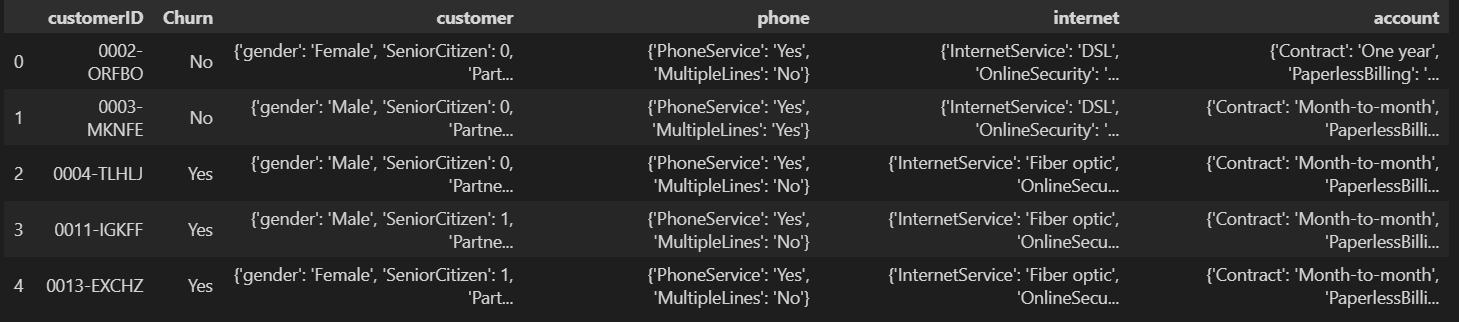But, as we can see, `customer`, `phone`, `internet`, and `account` are their separate tables. So I had to normalize them separately and then I just concatenated all these tables into one. ## Missing data The first time I looked for missing data in our dataset I notice that apparently, that wasn't anything missing, but later on, I noticed that there was empty space and just space not being counted as `NaN`. So I corrected this, and now the dataset had 224 missing values for `Churn` and 11 missing for `Charges.Total`. ``` customerID 0 Churn 224 gender 0 SeniorCitizen 0 Partner 0 Dependents 0 tenure 0 PhoneService 0 MultipleLines 0 InternetService 0 OnlineSecurity 0 OnlineBackup 0 DeviceProtection 0 TechSupport 0 StreamingTV 0 StreamingMovies 0 Contract 0 PaperlessBilling 0 PaymentMethod 0 Charges.Monthly 0 Charges.Total 11 dtype: int64 ``` I decided to drop the missing `Churn` because this is going to be the object of our study and there isn't a point in studying something that doesn't exist. For the missing `Charges.Total`, I think it represents a customer that hasn't paid anything yet, so I just replaced the missing value for 0. ## Feature Encoding The feature `SeniorCitizen` was the only one that came with `0` and `1` instead of `Yes` and `No`. For now, I'm changing it to yes and no, because it'll make the analysis simpler to read. 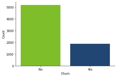# Second Week ## Data Analysis In the first plot, we can see how much unbalanced our data set is. There're over 5000 clients that didn't leave the company and a little less than 2000 that left.

I also generated 16 plots for all the discrete data. I wanted to see if there was any behavior that made some clients more likely to leave the company. To see all the plots look at the [notebook](https://github.com/devmedeiros/Challenge-Data-Science/blob/main/2%20-%20Data%20Analysis/data_analysis.ipynb) from `2 - Data Analysis`. Is easy to see that all, except for `gender`, seems to play a role in determining if a client will leave the company or not. More specifically payment methods, contracts, online backup, tech support, and internet service. 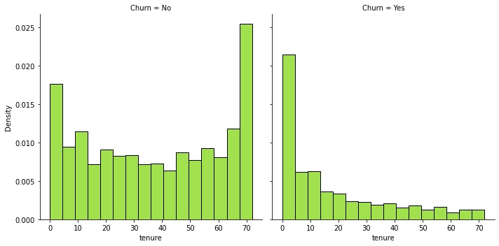In the `tenure` plot, I decided to make a distribution plot for the tenure, one plot for clients that didn't churn and clients that did churn. We can see that clients that left the company tend to do so at the beginning of their time in the company.

The average monthly charge for clients that didn't churn is 61.27 monetary units, while clients that churn were paying 74.44. This is probably because of the type of contract they prefer, but either way, is known that higher prices drive the customer away. ## The Churn Profile Considering everything that I could see through plots and measures I came up with a profile for clients that are more likely to churn. - New clients are more likely to churn than older clients. - Customers that use fewer services and products tend to leave the company. Also, when they aren't tied down to a longer contract they seem to be more likely to quit. - Regarding the payment method, clients that churn have a **strong** preference for electronic checks and usually are spending 13.17 monetary units more than the average client that didn't leave. # Third Week ## Preparing the dataset We start by making dummies variables dropping the first, so we would have n-1 dummies for n categories. Then we move on to look at features correlation.

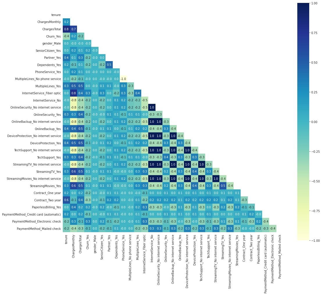
We can see that the `InternetService_No` feature has a lot of strong correlations with many other features, this is because these other features depend on the client having internet service. So I'll drop all features that are dependent on this one. The same thing happens with `PhoneService_Yes`. `tenure` and `ChargesTotal` also have a strong correlation, but I'll run the models with these two, as I think they are both relevant. After dropping these features I move on to normalize the numeric data, `ChargesTotal` and `tenure`. Because the dataset is so imbalanced, after splitting the dataset between training and testing sets, I'll oversample the training set using the SMOTE technique. ## Model Evaluation I'll use a dummy classifier to have a baseline model for the accuracy score, and I'll also use the metrics: `precision`, `recall` and `f1 score`. Although the dummy model won't have values for this metrics, I'll keep it for comparison on how much the models improved. ## Baseline I made the baseline model using a dummy classifier that guessed that every client behaved the same. It is always guessed that no client will leave the company. By using this approach we got a baseline accuracy score of `0.73456`. All models moving forward will have the same random state. ## Model 1 - Random Forest I start by using a grid search with cross-validation to find the best parameters within a given pool of options using the `recall` as the strategy to evaluate the performance. The best model was: ```python RandomForestClassifier(criterion='entropy', max_depth=5, max_leaf_nodes=70, random_state=22) ``` After fitting this model, the evaluating metrics were: - Accuracy Score: 0.72534 - Precision Score: 0.48922 - Recall Score: 0.78877 - F1 Score: 0.60389 ## Model 2 - Linear SVC For this model, I just used the default parameters and set the ceiling for the maximum of iterations to `900000`. ```python LinearSVC(max_iter=900000, random_state=22) ``` After fitting this model, the evaluating metrics were: - Accuracy Score: 0.71966 - Precision Score: 0.48217 - Recall Score: 0.75936 - F1 Score: 0.58982 ## Model 3 - Multi-layer Perceptron Here I fixed the solver to LBFGS and used grid search with cross-validation to find a hidden layer size that would be the best. The best model was: ```python MLPClassifier(hidden_layer_sizes=(1,), max_iter=9999, random_state=22, solver='lbfgs') ``` After fitting this model, the evaluating metrics were: - Accuracy Score: 0.72818 - Precision Score: 0.49133 - Recall Score: 0.68182 - F1 Score: 0.57111 ## Conclusion

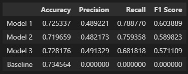
I ran three models, all of them using the same `random_state`. The first model was a random forest, with `max_depth = 5` and `max_leaf_nodes = 70`. I used grid search with cross-validation on some random parameters to find this combination and `recall` as the evaluating strategy for the cross-validation. The second model is a simple linear SVC. And lastly, the third model is a neural network with a multi-layer perceptron, in this case, I also used a grid search with cross-validation with LBFGS solver (because of the small dataset) on some random hidden layer sizes and `recall` as the evaluating strategy for the cross-validation. In the end, the Random Forest had the best metrics overall. # Fourth Week For the last week we're meant to work in the portfolio and storytelling. I wrote a blog post on my website that you can read more about it [here](https://bit.ly/38vJKUG).