{
"cells": [
{
"cell_type": "code",
"execution_count": 60,
"metadata": {},
"outputs": [],
"source": [
"using Plots, ComplexPhasePortrait, ApproxFun, SingularIntegralEquations\n",
"gr();"
]
},
{
"cell_type": "markdown",
"metadata": {},
"source": [
"# M3M6: Methods of Mathematical Physics\n",
"\n",
"$$\n",
"\\def\\dashint{{\\int\\!\\!\\!\\!\\!\\!-\\,}}\n",
"\\def\\infdashint{\\dashint_{\\!\\!\\!-\\infty}^{\\,\\infty}}\n",
"\\def\\D{\\,{\\rm d}}\n",
"\\def\\dx{\\D x}\n",
"\\def\\dt{\\D t}\n",
"\\def\\C{{\\mathbb C}}\n",
"\\def\\CC{{\\cal C}}\n",
"\\def\\HH{{\\cal H}}\n",
"\\def\\I{{\\rm i}}\n",
"\\def\\qqfor{\\qquad\\hbox{for}\\qquad}\n",
"$$\n",
"\n",
"Dr. Sheehan Olver\n",
"
\n",
"s.olver@imperial.ac.uk\n",
"\n",
"Office Hours: 3-4pm Mondays, Huxley 6M40\n",
"
\n",
"Website: https://github.com/dlfivefifty/M3M6LectureNotes\n",
"\n",
"# Lecture 19: Logarithmic singular integrals\n",
"\n",
"1. Evaluating logarithmic singular integrals\n",
"2. Logarithmic singular integrals and orthogonal polynomials\n",
"2. Solving a logarithmic singular integral equation\n",
"2. Application: electrostatic potentials in 2D\n",
" - Potential arising from a point charge and a single plate\n",
" \n",
"The motivation behind this lecture is to calculate electrostatic potentials. An example is the Faraday cage: imagine a series of metal plates connected together so that they have the same charge. If configured to surround a region, this configuration will shield the interior from an external charge:\n",
"\n",
"\n",
"\n",
"Here, the coloured lines are equipotential lines, and there is a point source at $x = 2$, which corresponds to a forcing of \n",
"$$\\log\\| (x,y) - (2,0) \\| = \\log|z - 2|$$\n",
"where $z = x + \\I y$. "
]
},
{
"cell_type": "markdown",
"metadata": {},
"source": [
"## Logarithmic singular integrals\n",
"\n",
"From the Green's function of the Laplacian, it is natural to consider logarithmic singular integrals, and we focus yet again on $[-1,1]$:\n",
"\n",
"$$v(z) = {1 \\over \\pi }\\int_{-1}^1 f(t) \\log | z - t| \\dt$$\n",
"\n",
"Note that off $[-1,1]$, $v(z)$ solves Laplace's equation, and is continuous on $[-1,1]$:"
]
},
{
"cell_type": "code",
"execution_count": 5,
"metadata": {},
"outputs": [
{
"data": {
"image/svg+xml": [
"\n",
"\n"
]
},
"execution_count": 5,
"metadata": {},
"output_type": "execute_result"
}
],
"source": [
"t = Fun()\n",
"f = sqrt(1-t^2)*exp(t)\n",
"v = z -> logkernel(f, z) # logkernel(f,z) calculates 1/π * \\int f(t)*log|t-z| dt\n",
"\n",
"xx = yy = -2:0.01:2\n",
"V = v.(xx' .+ im*yy)\n",
"\n",
"contour(xx, yy, V)\n",
"plot!(domain(t); color=:black, label=\"contour\")"
]
},
{
"cell_type": "code",
"execution_count": 6,
"metadata": {},
"outputs": [
{
"data": {
"image/svg+xml": [
"\n",
"\n"
]
},
"execution_count": 6,
"metadata": {},
"output_type": "execute_result"
}
],
"source": [
"surface(xx, yy, V)"
]
},
{
"cell_type": "markdown",
"metadata": {},
"source": [
"Continuity follows since $\\log|x-t|$ is integrable for $-1 \\leq x \\leq 1$ provided $f(t)$ has weaker than pole singularities. \n",
"\n",
"For $z \\notin (-\\infty,1]$ this can also be seen since $v$ is the real part of an analytic function:\n",
"$$\n",
" v(z) = \\Re {1 \\over \\pi} \\int_{-1}^1 f(t) \\log ( z - t) \\dt\n",
"$$\n",
"Note that the integrand avoids the branch cut of $\\log z$. To extend this to $z\\in (-\\infty,-1]$ (or more generally, $z \\notin [-1,\\infty)$), we can use the alternative expression\n",
"$$\n",
" v(z) = \\Re {1 \\over \\pi} \\int_{-1}^1 f(t) \\log (t-z) \\dt\n",
"$$\n",
"which follows from $\\log|z-t| = \\log|t-z|$."
]
},
{
"cell_type": "code",
"execution_count": 7,
"metadata": {},
"outputs": [
{
"name": "stdout",
"output_type": "stream",
"text": [
"v(z) = 0.7068168642791222\n",
"sum(f * log(abs(z - t))) / π = 0.7068168642791223\n",
"sum(f * log(z - t)) / π = 0.7068168642791222 + 0.5923597267719309im\n",
"sum(f * log(t - z)) / π = 0.7068168642791222 - 1.1831399624402499im\n"
]
}
],
"source": [
"z = 2.0 +3.0im\n",
"@show v(z)\n",
"@show sum(f*log(abs(z-t)))/π\n",
"@show sum(f*log(z-t))/π\n",
"@show sum(f*log(t-z))/π;"
]
},
{
"cell_type": "markdown",
"metadata": {},
"source": [
"### Evaluating logarithmic singular integrals\n",
"\n",
"How can we actually evaluate \n",
"$$\n",
"Lu(z) = {1 \\over \\pi} \\int_{-1}^1 u(t) \\log (z-t) \\dt\n",
"$$\n",
"for $z$ in the complex plane? We relate this to the indefinite integral of the Cauchy transform, and then use that to reduce it to a Cauchy transform itself.\n",
"\n",
"#### Integrated Cauchy transform\n",
"\n",
"For $z$ away from the branch cut our integrand is \"nice\" (assuming $u$ itself is \"nice\") and we can exchange integration and differentiation to determine\n",
"$$\n",
"{\\D \\over \\D z} Lu(z) = {1 \\over \\pi} \\int_{-1}^1 u(t) {1\\over z -t} \\dt = -2 \\I \\CC u(z)\n",
"$$\n",
"thus if we can calculate $\\int^z Cu(\\zeta) \\D \\zeta$, we are in good shape. \n",
"\n",
"\n",
"_Example_ If $u(x) = {1 \\over \\sqrt{1-x^2}}$, then recall\n",
"$$\n",
"Cu(z) = {-1 \\over 2 \\I \\sqrt{z-1} \\sqrt{z+1}}\n",
"$$\n",
"We therefore have\n",
"$$\n",
"{\\D \\over \\D z} Lu(z) = {1 \\over \\sqrt{z-1} \\sqrt{z+1}} \n",
"$$\n",
"and therefore for some constant of integration $D$ we have\n",
"$$\n",
"Lu(z) + D = \\pi \\int^z {\\D z \\over \\sqrt{z-1} \\sqrt{z+1}} = 2 \\pi \\log\\left(\\sqrt{z-1} + \\sqrt{z+1}\\right)\n",
"$$\n",
"We need the right constant of integration. we can find that via the behaviour as $x \\rightarrow \\infty$:\n",
"$$\n",
"Lu(x) ={1 \\over \\pi} \\int_{-1}^1 u(t) \\log(x-t) \\dt = {\\log x \\over \\pi} \\int_{-1}^1 u(t) \\dt + {1 \\over \\pi} \\int_{-1}^1 u(t) \\log(1-t/x) \\dt = {\\log x \\over \\pi}\\int_{-1}^1 u(t) \\dt + O(x^{-1})\n",
"$$\n",
"Since we have\n",
"$$\n",
"\\int_{-1}^1 {1 \\over \\sqrt{1-x^2}} \\dx = \\pi\n",
"$$\n",
"and\n",
"$$\n",
"2 \\log(\\sqrt{x-1} + \\sqrt{x+1}) = 2 \\log \\sqrt x + 2 \\log(\\sqrt{1-1/x} + \\sqrt{1 + 1/x}) = \n",
"\\pi \\log x + 2\\pi \\log(2) + O(1/x)\n",
"$$\n",
"therefore, \n",
"$$\n",
"Lu(z) = 2 \\log\\left(\\sqrt{z-1} + \\sqrt{z+1}\\right) - 2 \\log 2\n",
"$$\n",
"\n",
"_Demonstration_ We want to calculate the log kernel of $1/\\sqrt{1-x^2}$:"
]
},
{
"cell_type": "code",
"execution_count": 10,
"metadata": {},
"outputs": [
{
"data": {
"text/plain": [
"0.3681278813450904 + 0.9045568943023814im"
]
},
"execution_count": 10,
"metadata": {},
"output_type": "execute_result"
}
],
"source": [
"x = Fun()\n",
"u = 1/sqrt(1-t^2)\n",
"z = 1+im\n",
"sum(u*log(z-x))/π"
]
},
{
"cell_type": "markdown",
"metadata": {},
"source": [
"We saw that its derivative is given in terms of the Cauchy transform, here we test it using finite difference approximation:"
]
},
{
"cell_type": "code",
"execution_count": 17,
"metadata": {},
"outputs": [
{
"data": {
"text/plain": [
"(0.3515911336637867 - 0.5688482444998755im, 0.35157758425414287 - 0.5688644810057831im, 0.3515775842541429 - 0.568864481005783im)"
]
},
"execution_count": 17,
"metadata": {},
"output_type": "execute_result"
}
],
"source": [
"h = 0.0001;\n",
"(sum(u*log(z+h-x))/π - sum(u*log(z-x))/π)/h , sum(u/(z-x))/π, -2im*cauchy(u,z)"
]
},
{
"cell_type": "markdown",
"metadata": {},
"source": [
"But we already know the Cauchy transform in closed form:"
]
},
{
"cell_type": "code",
"execution_count": 22,
"metadata": {},
"outputs": [
{
"data": {
"text/plain": [
"0.3515775842541429 - 0.568864481005783im"
]
},
"execution_count": 22,
"metadata": {},
"output_type": "execute_result"
}
],
"source": [
"Cu = z -> -1/(2im*sqrt(z-1)sqrt(z+1))\n",
"\n",
"-2im*Cu(z)"
]
},
{
"cell_type": "markdown",
"metadata": {},
"source": [
"This we can integrate in closed form to determine:"
]
},
{
"cell_type": "code",
"execution_count": 24,
"metadata": {},
"outputs": [
{
"data": {
"text/plain": [
"0.36812788134509056 + 0.9045568943023812im"
]
},
"execution_count": 24,
"metadata": {},
"output_type": "execute_result"
}
],
"source": [
"Lu = z -> 2*log(sqrt(z-1) + sqrt(z+1)) - 2*log(2)\n",
"Lu(z)"
]
},
{
"cell_type": "markdown",
"metadata": {},
"source": [
"#### Reduction to a Cauchy transform\n",
"\n",
"The representation is not ideal as it involves indefinite integration in the complex plane. However, we will see that we can actually express $L u (z)$ as a Cauchy transform of $\\int_x^1 u(t) \\dt$. \n",
"\n",
"**Lemma (Log kernel as Cauchy transform)** Suppose $u$ is \"nice\" (as in Plemelj). Then \n",
"$$\n",
"Lu(z) = {\\log(z-a) \\over \\pi} \\int_a^b u(x) \\dx +2 \\I C U(z)\n",
"$$\n",
"where \n",
"$$\n",
"U(x) = \\int_x^b u(t) \\dt\n",
"$$\n",
"\n",
"**Proof**\n",
"\n",
"We use Plemelj to prove this result (of course!) and assume $[a,b] = [-1,1]$. Note that $Lu$ satisfies the following Riemann–Hilbert problem:\n",
"\n",
"1. $Lu(z) \\sim {1 \\over \\pi} \\int_{-1}^1 u(t) \\dt \\log z + o(1)$\n",
"2. $L^+ u(x) - L^- u(x) = 2 \\I \\int_x^1 u(t) \\dt $ for $-1 < x < 1$\n",
"3. $L^+ u(x) - L^- u(x) = 2\\I \\int_{-1}^1 u(t) \\dt $ for $x < -1$\n",
"\n",
"\n",
"The first part follows immediately by noting for $z \\rightarrow + \\infty$ we have \n",
"$$\\log(z - x) = \\log(z (1 - x/z)) = \\log z + \\log(1-x/z) = \\log z + o(1)$$\n",
"\n",
"We now see where the jumps come from. Since\n",
" $Lu'(z) = -2 \\I Cu(z)$ and\n",
" This let's us think of $Lu (z)$ as (2 is arbitrary here)\n",
"$$\n",
"L u(z) = Lu(2) + \\int_2^z C u (\\zeta) \\D\\zeta\n",
"$$\n",
"where the contour is a straight line (just like in the problem sheet for $\\log z$ that I'm sure everyone has done by now), but we can think of it also as an arc that avoids $[-1,1]$.\n",
"\n",
"Consider $x < -1$. Given an ellipse $\\gamma$ surrounding $[-1,1]$ we can write the integral representations and exchange orders to get: \n",
"$$\n",
"L u^+(x) - L u^-(x) = -2 \\I \\oint_\\gamma C u(\\zeta) \\D\\zeta = -2 \\I \\int_{-1}^1 u(t) {1\\over 2 \\pi \\I} \\oint_\\gamma {1 \\over t-z} \\dt \\D \\zeta = 2 \\I \\int_{-1}^1 u(t) \\dt \n",
"$$\n",
"\n",
"For $-1 < x < 1$, note that\n",
"$\n",
"L u(1) \n",
"$\n",
"is well-defined as there is only a logarithmic singularity times an algebraic one. Thus deforming the contour onto the interval we have \n",
"$$\n",
"L^\\pm u(x) = -2 \\I \\int_1^x C^\\pm u(t) \\dt + L u(1),\n",
"$$\n",
"hence\n",
"$$\n",
"L^+ u(x) -L^- u(x) = 2 \\I \\int_x^1 (C^+ u(t) - C^- u(t)) \\dt =2 \\I \\int_x^1 u(t) \\dt\n",
"$$\n",
"⬛️\n",
"\n",
"\n",
"\n",
"_Example_\n",
"For the problem above, we have that $\\int_x^1 {1 \\over \\sqrt{1-t^2}}\\dt = {\\rm arccos}\\, x$, which gives us:"
]
},
{
"cell_type": "code",
"execution_count": 37,
"metadata": {},
"outputs": [
{
"data": {
"text/plain": [
"(0.36812788134509017 + 0.9045568943023812im, 0.36812788134509056 + 0.9045568943023812im)"
]
},
"execution_count": 37,
"metadata": {},
"output_type": "execute_result"
}
],
"source": [
"x = Fun()\n",
"\n",
"u = 1/sqrt(1-x^2)\n",
"U = acos(x)\n",
"\n",
"\n",
"Lu = z -> 2*log(sqrt(z-1) + sqrt(z+1)) - 2*log(2)\n",
"\n",
"sum(u) * log(z+1)/π + sum(U/(x-z))/(π), Lu(z)"
]
},
{
"cell_type": "markdown",
"metadata": {},
"source": [
"# Log transforms of weighted orthogonal polynomials\n",
"\n",
"\n",
"Now consider ${1 \\over \\pi} \\int_a^b p_k(x) w(x) \\log |z-x| \\dx$, which we write in terms of the real part of\n",
"$$\n",
"L_k(z) = L[p_k w](z) = {1 \\over \\pi } \\int_a^b p_k(x) w(x) \\log (z-x) \\dx\n",
"$$"
]
},
{
"cell_type": "markdown",
"metadata": {},
"source": [
"For $k > 0$ we have $\\int_a^b p_k(x) w(x) dx = 0$ due to orthogonality, and hence we actually have no branch cut:"
]
},
{
"cell_type": "code",
"execution_count": 40,
"metadata": {},
"outputs": [
{
"data": {
"image/svg+xml": [
"\n",
"\n"
]
},
"execution_count": 40,
"metadata": {},
"output_type": "execute_result"
}
],
"source": [
"T₅ = Fun(Chebyshev(), [zeros(2);1])\n",
"w = 1/sqrt(1-x^2)\n",
"L₅ = z->cauchyintegral(w*T₅, z)\n",
"\n",
"phaseplot(-3..3, -3..3, L₅)"
]
},
{
"cell_type": "markdown",
"metadata": {},
"source": [
"\n",
"\n",
"#### Example: Weighted Chebyshev log transform\n",
"\n",
"For classical orthogonal polynomials we can go a step further and relate the indefinite integrals to other orthogonal polynomials.\n",
"\n",
" For example, recall that\n",
"$$\n",
"{\\D\\over \\dx}[\\sqrt{1-x^2} U_n(x)] = -{n+1 \\over \\sqrt{1-x^2}} T_{n+1}(x)\n",
"$$\n",
"in other words, \n",
"$$\n",
"\\int_x^1 {T_k(t) \\over \\sqrt{1-t^2}} \\dt = -{\\sqrt{1-x^2} U_{k-1}(x) \\over k}\n",
"$$\n",
"Thus for $k=1,2,\\ldots$,\n",
"$$\n",
"L_k(z) = -{1 \\over n+1} \\CC[\\sqrt{1-\\diamond^2} U_{k-1}](z)\n",
"$$\n",
"and\n",
"$$\n",
"{1 \\over \\pi} \\int_{-1}^1 {T_k(x) \\over \\sqrt{1-x^2}}\\log(z-x) \\dx = {2 \\I \\over k} \\CC[\\sqrt{1-\\diamond^2} U_{k-1}](z)\n",
"$$\n"
]
},
{
"cell_type": "code",
"execution_count": 42,
"metadata": {},
"outputs": [
{
"data": {
"text/plain": [
"(0.00018695792399762436 - 0.0009741971129007227im, 0.0001869579239976236 - 0.000974197112900722im)"
]
},
"execution_count": 42,
"metadata": {},
"output_type": "execute_result"
}
],
"source": [
"T₅ = Fun(Chebyshev(), [zeros(5);1])\n",
"U₄ = Fun(Ultraspherical(1), [zeros(4);1])\n",
"x = Fun()\n",
"L₅ = z->sum(T₅/sqrt(1-x^2) * log(z-x))/π\n",
"\n",
"L₅(z), 2im*cauchy(sqrt(1-x^2)*U₄,z)/5"
]
},
{
"cell_type": "markdown",
"metadata": {},
"source": [
"As we saw last lecture, Cauchy transforms of OPs satisfy simple recurrences, and this relationship renders log transforms equally calculable. "
]
},
{
"cell_type": "markdown",
"metadata": {},
"source": [
"\n",
"\n",
"### Solving logarithmic singular integral equations\n",
"\n",
"Oddly enough, it is easier to solve a singular integral equation involving the logarithmic kernel than to actually calculate the logarithmic singular integral, so we begin here. Consider the problem of calculating $u(x)$ such that\n",
"$$\n",
"{1 \\over \\pi} \\int_{-1}^1 u(t) \\log | x-t| \\dt = f(x) \\qqfor -1 < x < 1\n",
"$$\n",
"\n",
"\n",
"To tackle this problem we first need to understand the additive jump $Re L^\\pm(x) = {L^+(x) + L^-(x) \\over 2}$. Thinking in terms of integrals of Cauchy transforms we see that\n",
"$$\n",
"L^+u(x) + L^-u(x) = -2\\I (2\\int_2^1 \\CC u(x) \\dx + \\int_1^x [C^+ u(t) + C^-u(t)] \\dt) =\n",
" D -2 \\I \\int_1^x (-\\I H u(t)) \\dt = D + 2\\int_x^1 H u(t) dt\n",
"$$\n",
"That is, it is expressed as an indefinite integral of the Hilbert transform. We therefore have:\n",
"$$\n",
"{\\D \\over \\dx} {1 \\over \\pi} \\int_{-1}^1 u(t) \\log | x-t| \\dt = {\\D \\over \\dx} \\int_x^1 H u(t) dt = - Hu(x)\n",
"$$\n",
"where the minus sign comes from the fact that $x$ is the lower limit. In other words, our original SIE becomes equivalent to inverting the Hilbert transform:\n",
"$$\n",
"\\HH u(x) = -f'(x)\n",
"$$\n",
"recall, we can express the solution as\n",
"$$\n",
" u = {1 \\over \\sqrt{1-x^2}} \\HH[\\sqrt{1-\\diamond^2} f'] + {C\\over \\sqrt{1-x^2}}\n",
"$$\n",
"\n",
"Let's do a numerical example:"
]
},
{
"cell_type": "code",
"execution_count": 43,
"metadata": {},
"outputs": [
{
"name": "stdout",
"output_type": "stream",
"text": [
"hilbert(u, 0.1) + f(0.1) = -4.440892098500626e-16\n",
"logkernel(u, 0.1) - f(0.1) = -0.18115023187927326\n",
"logkernel(u, 0.2) - f(0.2) = -0.18115023187927304\n"
]
}
],
"source": [
"x = Fun()\n",
"f = exp(x)\n",
"\n",
"C = randn()\n",
"\n",
"u₁ = hilbert(sqrt(1-x^2)*f')/sqrt(1-x^2) \n",
"\n",
"u = u₁ + C/sqrt(1-x^2)\n",
"\n",
"@show hilbert(u, 0.1) + f(0.1)\n",
"@show logkernel(u,0.1) - f(0.1) # didn't work 😩\n",
"@show logkernel(u,0.2) - f(0.2); # but we are only off by a constant"
]
},
{
"cell_type": "markdown",
"metadata": {},
"source": [
"Remember: for inverting the Hilbert transform we had a degree of freedom: every solution plus $C/\\sqrt{1-x^2}$ was also a solution. But here, since we differentiated, we use that degree of freedom to ensure that we have arrived at the right solution. \n",
"\n",
"To choose $C$, we use the fact that\n",
"$$\n",
"f(0) = {1 \\over \\pi} \\int_{-1}^1 u(t) \\log |t| \\dt\n",
"$$\n",
"If we can calculate the right integral, we can use this to choose $C$:"
]
},
{
"cell_type": "code",
"execution_count": 44,
"metadata": {},
"outputs": [
{
"name": "stdout",
"output_type": "stream",
"text": [
"hilbert(u, 0.1) + f(0.1) = -4.440892098500626e-16\n",
"logkernel(u, 0.1) - f(0.1) = 0.0\n",
"logkernel(u, 0.2) - f(0.2) = 2.220446049250313e-16\n"
]
}
],
"source": [
"# choose C so that\n",
"# logkernel(u₁, 0) + C*logkernel(1/sqrt(1-x^2), 0) == f(0)\n",
"C = (f(0) - logkernel(u₁, 0))/logkernel(1/sqrt(1-x^2), 0)\n",
"u = u₁ + C/sqrt(1-x^2)\n",
"\n",
"@show hilbert(u, 0.1) + f(0.1)\n",
"@show logkernel(u,0.1) - f(0.1) # Works!\n",
"@show logkernel(u,0.2) - f(0.2); # And at all x!"
]
},
{
"cell_type": "markdown",
"metadata": {},
"source": [
"*Example* We now do an example which can be solved by hand. Find $u(x)$ so that: \n",
"$$\n",
"\\int_{-1}^1 u(t) \\log | x-t| \\dt = 1.\n",
"$$\n",
"Differentiating, we know that \n",
"$$\n",
"\\int_{-1}^1 {u(t) \\over x-t} \\dt = 0\n",
"$$\n",
"hence $u(x)$ must be of the form ${C \\over \\sqrt{1-x^2}}$. Which $C$? Make it work for $x = 0$:\n",
"$$\n",
"1 = \\int_{-1}^1 u(t) \\log | 0 - t| \\dt = C \\int_{-1}^1 {\\log | t| \\over \\sqrt{1-t^2}} \\dt\n",
"$$\n",
"To evaluate the integral, we can use trigonmetric variables:\n",
"$$\n",
"\\int_0^1 {\\log t \\over \\sqrt{1-t^2}} \\dt = \\int_0^{\\pi \\over 2} {\\cos \\theta \\log \\sin \\theta \\over \\sqrt{1-\\sin^2 \\theta}} \\D\\theta = \\int_0^{\\pi \\over 2} \\log \\sin \\theta \\D\\theta = - {\\pi \\log 2\\over 2}\n",
"$$\n",
"(The last identity takes some work: I'll leave it as an excercise.)\n",
"\n",
"Thus we have $ C = -{1 \\over \\pi \\log 2}$"
]
},
{
"cell_type": "code",
"execution_count": 49,
"metadata": {},
"outputs": [
{
"data": {
"text/plain": [
"1.0"
]
},
"execution_count": 49,
"metadata": {},
"output_type": "execute_result"
}
],
"source": [
"x = Fun()\n",
"C = -1/(log(2))\n",
"u = C/sqrt(1-x^2)\n",
"\n",
"logkernel(u, 0.2) "
]
},
{
"cell_type": "markdown",
"metadata": {},
"source": [
"Physically, this solution gives us the potential field \n",
"$$\n",
"\\int_{-1}^1 u(t) \\log|z-t| \\dt\n",
"$$\n",
"corresponding to holding a metal plate at constant potential:"
]
},
{
"cell_type": "code",
"execution_count": 52,
"metadata": {},
"outputs": [
{
"data": {
"image/svg+xml": [
"\n",
"\n"
]
},
"execution_count": 52,
"metadata": {},
"output_type": "execute_result"
}
],
"source": [
"v = z -> π*logkernel(u, z)\n",
"\n",
"xx = yy = -2:0.01:2\n",
"V = v.(xx' .+ im*yy)\n",
"\n",
"contour(xx, yy, V)\n",
"plot!(domain(x); color=:black)"
]
},
{
"cell_type": "code",
"execution_count": 53,
"metadata": {},
"outputs": [
{
"data": {
"image/svg+xml": [
"\n",
"\n"
]
},
"execution_count": 53,
"metadata": {},
"output_type": "execute_result"
}
],
"source": [
"surface(xx, yy, V)"
]
},
{
"cell_type": "markdown",
"metadata": {},
"source": [
"## Application: Potential arising from a point charge and a single plate\n",
"\n",
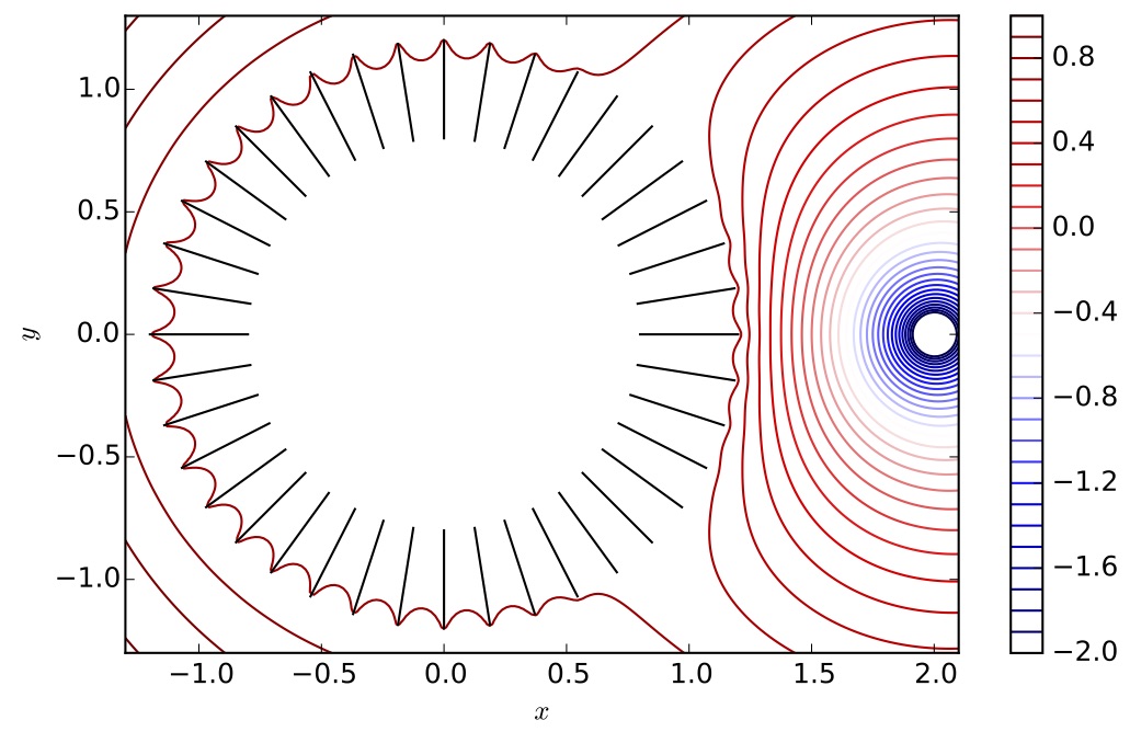
"Now imagine we put a point source at $x = 2$, and a metal plate on $[-1,1]$. We know the potential on the plate must be constant, but we don't know what constant. This is equivalent to the following problem (see e.g. [\\[Chapman, Hewett & Trefethen 2015\\]](https://people.maths.ox.ac.uk/trefethen/chapman_hewett_trefethen.pdf)):\n",
"\\begin{align*}\n",
"v_{xx} + v_{yy} = 0 &\\qqfor \\hbox{off $[-1,1]$ and $2$} \\\\\n",
"v(z) \\sim \\log |z - 2| + O(1) &\\qqfor z \\rightarrow 2 \\\\\n",
"v(z) \\sim \\log|z| + o(1) &\\qqfor z \\rightarrow \\infty \\\\\n",
"v(x) = \\kappa &\\qqfor -1 < x < 1\n",
"\\end{align*}\n",
"where $\\kappa$ is an unknown constant. We write the solution as\n",
"$$\n",
"v(z) = {1 \\over \\pi} \\int_{-1}^1 u(t) \\log|t-z| \\dt + \\log|z-2|\n",
"$$\n",
"for a to-be-determined $u$. On $-1 < x < 1$ this satisfies\n",
"$$\n",
" {1 \\over \\pi} \\int_{-1}^1 u(t) \\log|t-x| \\dt = \\kappa - \\log(2-x)\n",
"$$\n",
"\n",
"We can calculate the solution numerically as follows:"
]
},
{
"cell_type": "code",
"execution_count": 133,
"metadata": {},
"outputs": [
{
"data": {
"image/svg+xml": [
"\n",
"\n"
]
},
"execution_count": 133,
"metadata": {},
"output_type": "execute_result"
}
],
"source": [
"x = Fun()\n",
"u₀ = SingularIntegral(0) \\ (-log(2-x)) # solution with κ = 0\n",
"u = u₀ - sum(u₀)/(π*sqrt(1-x^2)) # ensure correct asymptotics\n",
"v = z -> logkernel(u, z) + log(abs(2-z))\n",
"xx = yy = -4:0.011:4\n",
"V = v.(xx' .+ im*yy)\n",
"\n",
"contour(xx, yy, V)\n",
"plot!(domain(x); color=:black, legend=false)"
]
},
{
"cell_type": "markdown",
"metadata": {},
"source": [
"We can solve this equation explicitly. By differentiating we see that $u$ satisfies the following:\n",
"$$\n",
"Hu(x) = -f'(x) = {1 \\over x-2}\n",
"$$\n",
"We now use the inverse Hilbert formula to determine:\n",
"$$\n",
"u(x) = -{1\\over\\sqrt{1-x^2}} H[{1 \\over \\diamond-2} \\sqrt{1-\\diamond^2}](x) + {D \\over \\sqrt{1-x^2}}\n",
"$$\n",
"Using the usual procedure of taking an obvious ansatz and subtracting off the singularities at poles and $\\infty$ we find that:\n",
"$$\n",
"C[{\\sqrt{1-\\diamond^2} \\over x -2}](z) = \\underbrace{\\sqrt{z-1} \\sqrt{z+1} \\over 2 \\I (z-2)}_{\\hbox{ansatz}} - \\underbrace{\\sqrt 3\\over 2 \\I (z-2)}_{\\hbox{remove pole near $z=2$}} - \\underbrace{{1 \\over 2 \\I}}_{\\hbox{remove constant at $\\infty$}}\n",
"$$\n",
"This implies that\n",
"$$\n",
"H[{1 \\over\\diamond-2} \\sqrt{1-\\diamond^2}](x) = \\I(C^+ + C^-)[{1 \\over\\diamond-2} \\sqrt{1-\\diamond^2}](x) = -{\\sqrt 3 \\over x -2} - 1\n",
"$$\n",
"in other words, \n",
"$$\n",
"u = {\\sqrt{3} \\over (x - 2) \\sqrt{1-x^2}} + {D \\over \\sqrt{1-x^2}}\n",
"$$\n",
"We still need to determine $D$. This is chosen so that we tend to $\\log |z|$ near $\\infty$. In particular, we know that\n",
"$$\n",
"{1 \\over \\pi} \\int_{-1}^1 \\log|z-x| u(x) \\dx \\sim {\\int_{-1}^1 u(x) \\dx \\over \\pi} \\log |z|\n",
"$$\n",
"so we need to choose $D$ so that $\\int_{-1}^1 u(x) \\dx = 0$ and only the $\\log|z-2|$ singularity appears near $\\infty$. We first note that \n",
"\\begin{align*}\n",
"C[{1 \\over (\\diamond - 2) \\sqrt{1-\\diamond^2}}](z) &= \\underbrace{{\\I \\over 2 \\sqrt{z-1} \\sqrt{z+1} (z-2)}}_{\\hbox{ansatz}} - \\underbrace{{\\I \\over 2\\sqrt{3} (z-2)}}_{\\hbox{remove pole}} \\\\\n",
"& = -{\\I \\over 2 \\sqrt{3} z} + O(z^{-2})\n",
"\\end{align*}\n",
"near $\\infty$. Since \n",
"$$\n",
"Cw(z) ={ \\int_{-1}^1 w(x) \\dx \\over -2\\pi \\I z} + O(z^{-2}) \n",
"$$\n",
"we can infer the integral from the Cauchy transform and find that\n",
"$$\n",
"\\int_{-1}^1 {1 \\over (x - 2) \\sqrt{1-x^2}} \\dx = -{ \\pi \\over \\sqrt{3}}\n",
"$$\n",
"On the other hand,\n",
"$$\n",
"\\int_{-1}^1 {\\dx \\over \\sqrt{1-x^2}} = \\pi\n",
"$$\n",
"Thus we require $D = 1$ and have the solution:\n",
"$$\n",
"u(x) = {\\sqrt{3} \\over (x - 2) \\sqrt{1-x^2}} - {1 \\over \\sqrt{1-x^2}}\n",
"$$"
]
},
{
"cell_type": "markdown",
"metadata": {},
"source": [
"_Demonstration_ We first check that differentiation reduces to the Hilbert transform:"
]
},
{
"cell_type": "code",
"execution_count": 149,
"metadata": {},
"outputs": [
{
"data": {
"text/plain": [
"true"
]
},
"execution_count": 149,
"metadata": {},
"output_type": "execute_result"
}
],
"source": [
"t = Fun()\n",
"f = -log(2-t)\n",
"hilbert(u, 0.1) ≈ -f'(0.1) ≈ 1/(0.1-2)"
]
},
{
"cell_type": "markdown",
"metadata": {},
"source": [
"In the inverse Hilbert transform we calculated the following Cauchy transform:"
]
},
{
"cell_type": "code",
"execution_count": 150,
"metadata": {},
"outputs": [
{
"data": {
"text/plain": [
"true"
]
},
"execution_count": 150,
"metadata": {},
"output_type": "execute_result"
}
],
"source": [
"z = 1+im\n",
"cauchy((-f')*sqrt(1-t^2), z) ≈ sqrt(z-1)sqrt(z+1)/(2im*(z-2)) - sqrt(3)/(2im*(z-2)) - 1/(2im)"
]
},
{
"cell_type": "markdown",
"metadata": {},
"source": [
"Which means that:"
]
},
{
"cell_type": "code",
"execution_count": 153,
"metadata": {},
"outputs": [
{
"data": {
"text/plain": [
"(-0.08839431180585401, -0.08839431180585411)"
]
},
"execution_count": 153,
"metadata": {},
"output_type": "execute_result"
}
],
"source": [
"hilbert((-f')*sqrt(1-t^2), 0.1), -sqrt(3)/(0.1-2) - 1"
]
},
{
"cell_type": "markdown",
"metadata": {},
"source": [
"Thus we have the inverse Hilbert transform:"
]
},
{
"cell_type": "code",
"execution_count": 140,
"metadata": {},
"outputs": [
{
"data": {
"text/plain": [
"true"
]
},
"execution_count": 140,
"metadata": {},
"output_type": "execute_result"
}
],
"source": [
"D = randn()\n",
"ũ = sqrt(3)/((x-2)*sqrt(1-x^2)) + D/sqrt(1-x^2)\n",
"hilbert(ũ,0.1) ≈ -f'(0.1)"
]
},
{
"cell_type": "markdown",
"metadata": {},
"source": [
"We still need to determine the constant $D$. What goes wrong if we have the wrong choice is that we don't tend to precisely $\\log z$ near $\\infty$:"
]
},
{
"cell_type": "code",
"execution_count": 141,
"metadata": {},
"outputs": [
{
"data": {
"text/plain": [
"(-24.76573192820616, 12.206072645530174)"
]
},
"execution_count": 141,
"metadata": {},
"output_type": "execute_result"
}
],
"source": [
"z = 200000\n",
"logkernel(ũ,z), log(z)"
]
},
{
"cell_type": "markdown",
"metadata": {},
"source": [
"We determined the integral"
]
},
{
"cell_type": "code",
"execution_count": 142,
"metadata": {},
"outputs": [
{
"data": {
"text/plain": [
"true"
]
},
"execution_count": 142,
"metadata": {},
"output_type": "execute_result"
}
],
"source": [
"sum(1/((x-2)*sqrt(1-x^2))) ≈ -2π/(2*sqrt(3))"
]
},
{
"cell_type": "markdown",
"metadata": {},
"source": [
"Therefore:"
]
},
{
"cell_type": "code",
"execution_count": 160,
"metadata": {},
"outputs": [
{
"data": {
"text/plain": [
"1.743934249004316e-16"
]
},
"execution_count": 160,
"metadata": {},
"output_type": "execute_result"
}
],
"source": [
"sum(u)"
]
},
{
"cell_type": "markdown",
"metadata": {},
"source": [
"We thus found $u$:"
]
},
{
"cell_type": "code",
"execution_count": 154,
"metadata": {},
"outputs": [
{
"data": {
"text/plain": [
"(0.08883962601869715, 0.08883962601869722)"
]
},
"execution_count": 154,
"metadata": {},
"output_type": "execute_result"
}
],
"source": [
"x = 0.1; u(x), sqrt(3)/((x-2)*sqrt(1-x^2)) + 1/sqrt(1-x^2)"
]
}
],
"metadata": {
"kernelspec": {
"display_name": "Julia 1.0.0",
"language": "julia",
"name": "julia-1.0"
},
"language_info": {
"file_extension": ".jl",
"mimetype": "application/julia",
"name": "julia",
"version": "1.0.0"
}
},
"nbformat": 4,
"nbformat_minor": 2
}