{
"cells": [
{
"cell_type": "markdown",
"metadata": {},
"source": [
"# Build Your Own TensorFlow!\n",
"\n",
"In this lab, you’ll build a library called miniflow which will be your own version of [TensorFlow](http://tensorflow.org/)! TensorFlow is one of the most popular open source neural network libraries, built by the team at Google Brain just over the last few years. Through building this lab, you’ll be able to better understand backpropagation, the engine behind neural networks. We’ll finally use this library that you built to [classify digits in handwriting](http://yann.lecun.com/exdb/mnist/)! This will be a very hands on and interactive experience - let’s get started!"
]
},
{
"cell_type": "markdown",
"metadata": {},
"source": [
"## Intro"
]
},
{
"cell_type": "markdown",
"metadata": {},
"source": [
"Following this lab, all other neural network type of activities will done with [TensorFlow](http://tensorflow.org/) and [higher-level APIs](https://keras.io/) in its ecosystem. So why bother with this lab then? Good question, glad you asked!\n",
"\n",
"The goal of this lab is to demystify two concepts at the heart of network networks - backpropagation and differentiable graphs. Backpropagation is the process by which we update the weight of our network over time. You may have seen it in [this video](https://classroom.udacity.com/nanodegrees/nd013/parts/fbf77062-5703-404e-b60c-95b78b2f3f9e/modules/6df7ae49-c61c-4bb2-a23e-6527e69209ec/lessons/59e94b37-ef38-43ff-acd4-4c7f5326cff5/concepts/4320886810923#) in the previous lesson. Differentiable graphs are graphs where the nodes are [differentiable functions](https://en.wikipedia.org/wiki/Differentiable_function). They are also very useful as a *visual aid* for understanding and calculating complicated derivatives. This is the fundamental abstraction of TensorFlow, it's a framework for creating these type of graphs. With this understanding, we will be able to create our own nodes and properly compute the derivatives. Even more importantly, we will be able to think and reason in terms of these graphs.\n",
"\n",
"By the end of this lab, miniflow will be able to recognize the digit in an image of handwritten digit. This is a pretty neat result that you’ll build from scratch!\n",
"\n",
"Now. Let's take our first peek under the hood ..."
]
},
{
"cell_type": "markdown",
"metadata": {},
"source": [
"## Neural Networks, Backpropagation and the Chain Rule"
]
},
{
"cell_type": "markdown",
"metadata": {},
"source": [
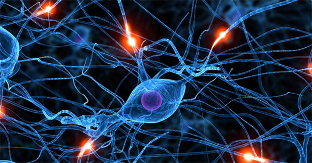
"So neural networks sound pretty intimidating right? I mean, it's supposed to be based off our brains, and nobody knows how those things work!\n",
"\n",
" \n",
"\n",
"Luckily, neural networks are very loosely based off our brains and the core abstractions behind how they work are actually much simpler than you would think. They look more than this: \n",
"\n",
"
\n",
"\n",
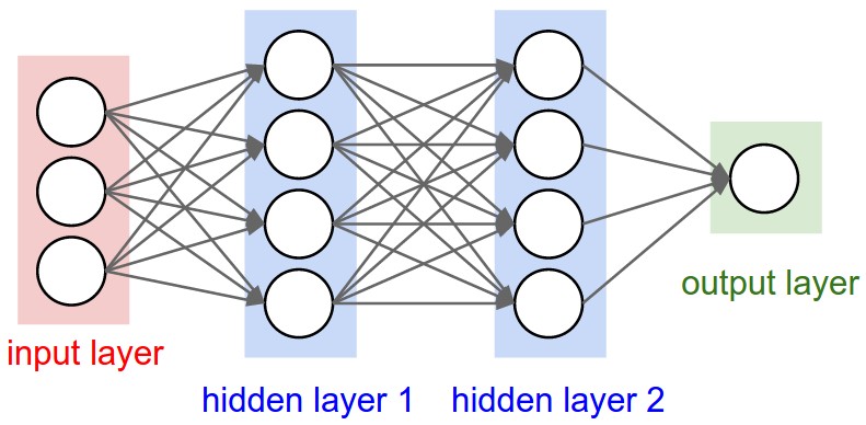
"Luckily, neural networks are very loosely based off our brains and the core abstractions behind how they work are actually much simpler than you would think. They look more than this: \n",
"\n",
" \n",
"\n",
"So how does a neural network work? Let's first break up the neural network in into components, we have:\n",
"\n",
"1. **Inputs**. This can be our data(features/labels) and weights\n",
"2. **Functions**. The neural network itself is essentially a chain or composition of functions.\n",
"3. **Output**. This is the final output of the neural network before it's fed into the loss function. If we're doing classification it's this will be a number signifying the class. If it's regression, this will be a number of some value (ex: house price if we're predicted house prices).\n",
"4. **Loss Function**. This function compares our output (3) with the correct label or value and itself returns another number. This number is called the loss. Typically we'll restrict the loss to be either a positive number, in which case we minimize the value, or, a negative number, in which case we maximize. Either way we're approaching 0.\n",
"\n",
"Let's say we want to minimize the loss. How do we do that?\n",
"\n",
"Well, what do we have control of? Our inputs? Nope. Our inputs are the data which itself can vary significantly on the same dataset, but, we could also change our dataset entirely. We need something that sticks around, something stateful that also affects the output. \n",
"\n",
"What about our weights? \n",
"\n",
"Yes, That's exactly it! We can change our weights. They stay static unless we change them. Alright, now we have another question.\n",
"\n",
"How do we alter our weights?\n",
"\n",
"Intuitively we'd like to see what effect a weight had on the loss and make a change based on that. If it played a large role in the error then we should alter it by a large amount. If it didn't play a significant role in the error, then it's probably already set to a good value and we should, for the most part, let it be.\n",
"\n",
"How can we formalize this idea?\n",
"\n",
"Luckily for us, this idea is already well established in mathematical literature where it's known as **reverse-mode differentiation** or **backpropagation**. The name sounds very scary but it's actually not so bad. It essentially boils down to computing derivatives and using the chain rule. For example, say we wanted to compute the gradient of the $loss$ with respect to a weight $W^1_{kj}$. Here $W^1$ is a matrix of weights so $W^1_{kj}$ is an individual weight (number) at row $k$, column $j$ of $W^1$. Let's assume $W^1$ is an input/argument to the function $f_1$, meaning $f_1$ does some computation with $W^1$, the exact computation doesn't matter right now.\n",
"\n",
"$$\n",
"predictions = f_4(f_3(f_2(f_1(features, W^1)), W^3))\n",
"$$\n",
"\n",
"$L$ is the loss function.\n",
"\n",
"$$\n",
"loss = L(predictions, labels)\n",
"$$\n",
"\n",
"Using the [chain rule](https://www.khanacademy.org/math/ap-calculus-ab/product-quotient-chain-rules-ab/chain-rule-ab/a/chain-rule-overview) the computation is:\n",
"\n",
"$$\n",
"\\frac{\\partial L}{\\partial W^1_{kj}} = \n",
"\\frac{\\partial L}{\\partial f_4}\n",
"\\frac{\\partial f_4}{\\partial f_3}\n",
"\\frac{\\partial f_3}{\\partial f_2}\n",
"\\frac{\\partial f_2}{\\partial f_1}\n",
"\\frac{\\partial f_1}{\\partial W^1_{kj}}\n",
"$$\n",
"\n",
"#### Quick Aside: Notation\n",
"\n",
"You may have noticed in the above link they used the following notation:\n",
"\n",
"$$\n",
"\\frac {d}{dx} f(g(x)) = f'(g(x))g'(x)\n",
"$$\n",
"\n",
"This is equivalent to:\n",
"\n",
"$$\n",
"\\frac {\\partial f}{\\partial x} = \n",
"\\frac {\\partial f}{\\partial g} \\frac {\\partial g} {\\partial x}\n",
"$$\n",
"\n",
"The latter notation is used when we talk about *partial derivatives*, that is, we want measure the effect a specific input had on our output. This is precisely what we're going to be doing throughout this lab so we'll use the latter notation. By the way, the $\\partial$ symbol is called a *partial*. \n",
"\n",
"Ok, now back to our our friend $\\frac{\\partial L}{\\partial W^1_{kj}}$. This is mathematical speak for, \"what effect did weight $W^1_{kj}$ have on the output $L$?\" You might be wondering why we need to know all these other partials. Why can't we just write:\n",
"\n",
"$$\n",
"\\frac{\\partial L}{\\partial W^1_{kj}} = \n",
"\\frac{\\partial L}{\\partial f_1}\n",
"\\frac{\\partial f_1}{\\partial W^1_{kj}}\n",
"$$\n",
"\n",
"since $W^1_{kj}$ is the input to $f_1$.\n",
"\n",
"If we did that we would miss out on a wealth of information and most likely get an incorrect gradient. Remember that $f_1$ affects $f_2$ and $f_3$ affects $f_4$. Missing out on how all these intermediate functions affect each other won't do us any good and it'll only get worse the more intermediate functions we have.\n",
"\n",
"So in a sense we can write:\n",
"\n",
"$$\n",
"\\frac{\\partial L}{\\partial W^1_{kj}} = \n",
"\\frac{\\partial L}{\\partial f_1}\n",
"\\frac{\\partial f_1}{\\partial W^1_{kj}}\n",
"$$\n",
"\n",
"but just remember that:\n",
"\n",
"$$\n",
"\\frac{\\partial L}{\\partial f_1} =\n",
"\\frac{\\partial L}{\\partial f_4}\n",
"\\frac{\\partial f_4}{\\partial f_3}\n",
"\\frac{\\partial f_3}{\\partial f_2}\n",
"\\frac{\\partial f_2}{\\partial f_1}\n",
"$$\n",
"\n",
"otherwise we'll have a bad time!\n",
"\n",
"Ok, that's a lot of abstract thinking let's now take a look at a concrete example and practice taking partial derivatives."
]
},
{
"cell_type": "markdown",
"metadata": {},
"source": [
"### Case study: A simple function: $f = (x * y) + (x * z)$"
]
},
{
"cell_type": "markdown",
"metadata": {},
"source": [
"$$\n",
"mul(x,y) = x * y\n",
"$$\n",
"\n",
"$$\n",
"\\frac{\\partial mul}{\\partial x} = y \\hspace{0.5in} \\frac{\\partial mul}{\\partial y} = x\n",
"$$\n",
"\n",
"Let's think about this for a bit. What we're saying here is the change of $mul$ with respect to $x$ is $y$ and vice-versa. Remember, if our derivative is with respect to $x$, then we treat $y$ as a constant. \n",
"\n",
"Let's set $y = 10$. Now think about changing $x$ from 3 to 4. Then $mul(3,10) = 30$ and $mul(4, 10) = 40$. That's a change in 10 or $y$! Every time we change $x$ by 1, $mul$ changes by $y$.\n"
]
},
{
"cell_type": "markdown",
"metadata": {},
"source": [
"Here's a new example:\n",
"\n",
"$$\n",
"add(x,y) = x + y\n",
"$$\n",
"\n",
"$$\n",
"\\frac{\\partial add}{\\partial x} = 1 \\hspace{0.5in} \\frac{\\partial add}{\\partial y} = 1\n",
"$$\n",
"\n",
"Again, let's think about this. The change in $add$ with respect to $x$ is 1 and same for $y$. This means every time we change $x$ by 1, $add$ will also change by 1. This also shows $x$ and $y$ are independent of each other.\n",
"\n",
"Ok, let's now use this for a simple function."
]
},
{
"cell_type": "code",
"execution_count": 1,
"metadata": {
"collapsed": false
},
"outputs": [
{
"name": "stdout",
"output_type": "stream",
"text": [
"-3\n"
]
}
],
"source": [
"# f(x, y, z) = x * y + (x * z)\n",
"# we can split these into subexpressions\n",
"# g(x, y) = x * y\n",
"# h(x, z) = x * z\n",
"# f(x, y, z) = g(x, y) + h(x, z)\n",
"\n",
"# initial values\n",
"x = 3\n",
"y = 4\n",
"z = -5\n",
"\n",
"g = x * y\n",
"h = x * z\n",
"\n",
"f = g + h\n",
"print(f)"
]
},
{
"cell_type": "markdown",
"metadata": {},
"source": [
"Let's take our function $f$ and apply the chain rule to compute the derivatives for $x, y, z$.\n",
"\n",
"$$\n",
"\\frac{\\partial f}{\\partial g} = 1 \\hspace{0.1in}\n",
"\\frac{\\partial f}{\\partial h} = 1 \\hspace{0.1in}\n",
"\\frac{\\partial g}{\\partial x} = y \\hspace{0.1in}\n",
"\\frac{\\partial g}{\\partial y} = x \\hspace{0.1in}\n",
"\\frac{\\partial h}{\\partial x} = z \\hspace{0.1in}\n",
"\\frac{\\partial h}{\\partial z} = x\n",
"$$\n",
"\n",
"\n",
"$$\n",
"\\frac{\\partial f}{\\partial x} = \n",
"\\frac{\\partial f}{\\partial g}\n",
"\\frac{\\partial g}{\\partial x}\n",
"+\n",
"\\frac{\\partial f}{\\partial h}\n",
"\\frac{\\partial h}{\\partial x}\n",
"\\hspace{0.5in}\n",
"\\frac{\\partial f}{\\partial y} = \n",
"\\frac{\\partial f}{\\partial g}\n",
"\\frac{\\partial g}{\\partial y}\n",
"\\hspace{0.5in}\n",
"\\frac{\\partial f}{\\partial z} = \n",
"\\frac{\\partial f}{\\partial h}\n",
"\\frac{\\partial h}{\\partial z}\n",
"$$\n",
"\n",
"\n",
"$$\n",
"\\frac{\\partial f}{\\partial x} = 1 * y + 1 * z = y + z\n",
"\\hspace{0.5in}\n",
"\\frac{\\partial f}{\\partial y} = 1 * x = x\n",
"\\hspace{0.5in}\n",
"\\frac{\\partial f}{\\partial z} = 1 * x = x\n",
"$$"
]
},
{
"cell_type": "code",
"execution_count": 2,
"metadata": {
"collapsed": false
},
"outputs": [
{
"name": "stdout",
"output_type": "stream",
"text": [
"[-1.0, 3.0, 3.0]\n"
]
}
],
"source": [
"# The above in code\n",
"x = 3\n",
"y = 4\n",
"z = -5\n",
"\n",
"dfdg = 1.0\n",
"dfdh = 1.0\n",
"dgdx = y\n",
"dgdy = x\n",
"dhdx = z\n",
"dhdz = x\n",
"\n",
"dfdx = dfdg * dgdx + dfdh * dhdx\n",
"dfdy = dfdg * dgdy\n",
"dfdz = dfdh * dhdz\n",
"\n",
"# the output of backpropagation is the gradient\n",
"# TODO: what's the gradient?\n",
"gradient = [dfdx, dfdy, dfdz]\n",
"print(gradient) # should be [-1, 3, 3]"
]
},
{
"cell_type": "markdown",
"metadata": {},
"source": [
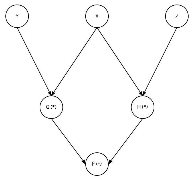
"Here's $f$ visually:\n",
"\n",
"
\n",
"\n",
"So how does a neural network work? Let's first break up the neural network in into components, we have:\n",
"\n",
"1. **Inputs**. This can be our data(features/labels) and weights\n",
"2. **Functions**. The neural network itself is essentially a chain or composition of functions.\n",
"3. **Output**. This is the final output of the neural network before it's fed into the loss function. If we're doing classification it's this will be a number signifying the class. If it's regression, this will be a number of some value (ex: house price if we're predicted house prices).\n",
"4. **Loss Function**. This function compares our output (3) with the correct label or value and itself returns another number. This number is called the loss. Typically we'll restrict the loss to be either a positive number, in which case we minimize the value, or, a negative number, in which case we maximize. Either way we're approaching 0.\n",
"\n",
"Let's say we want to minimize the loss. How do we do that?\n",
"\n",
"Well, what do we have control of? Our inputs? Nope. Our inputs are the data which itself can vary significantly on the same dataset, but, we could also change our dataset entirely. We need something that sticks around, something stateful that also affects the output. \n",
"\n",
"What about our weights? \n",
"\n",
"Yes, That's exactly it! We can change our weights. They stay static unless we change them. Alright, now we have another question.\n",
"\n",
"How do we alter our weights?\n",
"\n",
"Intuitively we'd like to see what effect a weight had on the loss and make a change based on that. If it played a large role in the error then we should alter it by a large amount. If it didn't play a significant role in the error, then it's probably already set to a good value and we should, for the most part, let it be.\n",
"\n",
"How can we formalize this idea?\n",
"\n",
"Luckily for us, this idea is already well established in mathematical literature where it's known as **reverse-mode differentiation** or **backpropagation**. The name sounds very scary but it's actually not so bad. It essentially boils down to computing derivatives and using the chain rule. For example, say we wanted to compute the gradient of the $loss$ with respect to a weight $W^1_{kj}$. Here $W^1$ is a matrix of weights so $W^1_{kj}$ is an individual weight (number) at row $k$, column $j$ of $W^1$. Let's assume $W^1$ is an input/argument to the function $f_1$, meaning $f_1$ does some computation with $W^1$, the exact computation doesn't matter right now.\n",
"\n",
"$$\n",
"predictions = f_4(f_3(f_2(f_1(features, W^1)), W^3))\n",
"$$\n",
"\n",
"$L$ is the loss function.\n",
"\n",
"$$\n",
"loss = L(predictions, labels)\n",
"$$\n",
"\n",
"Using the [chain rule](https://www.khanacademy.org/math/ap-calculus-ab/product-quotient-chain-rules-ab/chain-rule-ab/a/chain-rule-overview) the computation is:\n",
"\n",
"$$\n",
"\\frac{\\partial L}{\\partial W^1_{kj}} = \n",
"\\frac{\\partial L}{\\partial f_4}\n",
"\\frac{\\partial f_4}{\\partial f_3}\n",
"\\frac{\\partial f_3}{\\partial f_2}\n",
"\\frac{\\partial f_2}{\\partial f_1}\n",
"\\frac{\\partial f_1}{\\partial W^1_{kj}}\n",
"$$\n",
"\n",
"#### Quick Aside: Notation\n",
"\n",
"You may have noticed in the above link they used the following notation:\n",
"\n",
"$$\n",
"\\frac {d}{dx} f(g(x)) = f'(g(x))g'(x)\n",
"$$\n",
"\n",
"This is equivalent to:\n",
"\n",
"$$\n",
"\\frac {\\partial f}{\\partial x} = \n",
"\\frac {\\partial f}{\\partial g} \\frac {\\partial g} {\\partial x}\n",
"$$\n",
"\n",
"The latter notation is used when we talk about *partial derivatives*, that is, we want measure the effect a specific input had on our output. This is precisely what we're going to be doing throughout this lab so we'll use the latter notation. By the way, the $\\partial$ symbol is called a *partial*. \n",
"\n",
"Ok, now back to our our friend $\\frac{\\partial L}{\\partial W^1_{kj}}$. This is mathematical speak for, \"what effect did weight $W^1_{kj}$ have on the output $L$?\" You might be wondering why we need to know all these other partials. Why can't we just write:\n",
"\n",
"$$\n",
"\\frac{\\partial L}{\\partial W^1_{kj}} = \n",
"\\frac{\\partial L}{\\partial f_1}\n",
"\\frac{\\partial f_1}{\\partial W^1_{kj}}\n",
"$$\n",
"\n",
"since $W^1_{kj}$ is the input to $f_1$.\n",
"\n",
"If we did that we would miss out on a wealth of information and most likely get an incorrect gradient. Remember that $f_1$ affects $f_2$ and $f_3$ affects $f_4$. Missing out on how all these intermediate functions affect each other won't do us any good and it'll only get worse the more intermediate functions we have.\n",
"\n",
"So in a sense we can write:\n",
"\n",
"$$\n",
"\\frac{\\partial L}{\\partial W^1_{kj}} = \n",
"\\frac{\\partial L}{\\partial f_1}\n",
"\\frac{\\partial f_1}{\\partial W^1_{kj}}\n",
"$$\n",
"\n",
"but just remember that:\n",
"\n",
"$$\n",
"\\frac{\\partial L}{\\partial f_1} =\n",
"\\frac{\\partial L}{\\partial f_4}\n",
"\\frac{\\partial f_4}{\\partial f_3}\n",
"\\frac{\\partial f_3}{\\partial f_2}\n",
"\\frac{\\partial f_2}{\\partial f_1}\n",
"$$\n",
"\n",
"otherwise we'll have a bad time!\n",
"\n",
"Ok, that's a lot of abstract thinking let's now take a look at a concrete example and practice taking partial derivatives."
]
},
{
"cell_type": "markdown",
"metadata": {},
"source": [
"### Case study: A simple function: $f = (x * y) + (x * z)$"
]
},
{
"cell_type": "markdown",
"metadata": {},
"source": [
"$$\n",
"mul(x,y) = x * y\n",
"$$\n",
"\n",
"$$\n",
"\\frac{\\partial mul}{\\partial x} = y \\hspace{0.5in} \\frac{\\partial mul}{\\partial y} = x\n",
"$$\n",
"\n",
"Let's think about this for a bit. What we're saying here is the change of $mul$ with respect to $x$ is $y$ and vice-versa. Remember, if our derivative is with respect to $x$, then we treat $y$ as a constant. \n",
"\n",
"Let's set $y = 10$. Now think about changing $x$ from 3 to 4. Then $mul(3,10) = 30$ and $mul(4, 10) = 40$. That's a change in 10 or $y$! Every time we change $x$ by 1, $mul$ changes by $y$.\n"
]
},
{
"cell_type": "markdown",
"metadata": {},
"source": [
"Here's a new example:\n",
"\n",
"$$\n",
"add(x,y) = x + y\n",
"$$\n",
"\n",
"$$\n",
"\\frac{\\partial add}{\\partial x} = 1 \\hspace{0.5in} \\frac{\\partial add}{\\partial y} = 1\n",
"$$\n",
"\n",
"Again, let's think about this. The change in $add$ with respect to $x$ is 1 and same for $y$. This means every time we change $x$ by 1, $add$ will also change by 1. This also shows $x$ and $y$ are independent of each other.\n",
"\n",
"Ok, let's now use this for a simple function."
]
},
{
"cell_type": "code",
"execution_count": 1,
"metadata": {
"collapsed": false
},
"outputs": [
{
"name": "stdout",
"output_type": "stream",
"text": [
"-3\n"
]
}
],
"source": [
"# f(x, y, z) = x * y + (x * z)\n",
"# we can split these into subexpressions\n",
"# g(x, y) = x * y\n",
"# h(x, z) = x * z\n",
"# f(x, y, z) = g(x, y) + h(x, z)\n",
"\n",
"# initial values\n",
"x = 3\n",
"y = 4\n",
"z = -5\n",
"\n",
"g = x * y\n",
"h = x * z\n",
"\n",
"f = g + h\n",
"print(f)"
]
},
{
"cell_type": "markdown",
"metadata": {},
"source": [
"Let's take our function $f$ and apply the chain rule to compute the derivatives for $x, y, z$.\n",
"\n",
"$$\n",
"\\frac{\\partial f}{\\partial g} = 1 \\hspace{0.1in}\n",
"\\frac{\\partial f}{\\partial h} = 1 \\hspace{0.1in}\n",
"\\frac{\\partial g}{\\partial x} = y \\hspace{0.1in}\n",
"\\frac{\\partial g}{\\partial y} = x \\hspace{0.1in}\n",
"\\frac{\\partial h}{\\partial x} = z \\hspace{0.1in}\n",
"\\frac{\\partial h}{\\partial z} = x\n",
"$$\n",
"\n",
"\n",
"$$\n",
"\\frac{\\partial f}{\\partial x} = \n",
"\\frac{\\partial f}{\\partial g}\n",
"\\frac{\\partial g}{\\partial x}\n",
"+\n",
"\\frac{\\partial f}{\\partial h}\n",
"\\frac{\\partial h}{\\partial x}\n",
"\\hspace{0.5in}\n",
"\\frac{\\partial f}{\\partial y} = \n",
"\\frac{\\partial f}{\\partial g}\n",
"\\frac{\\partial g}{\\partial y}\n",
"\\hspace{0.5in}\n",
"\\frac{\\partial f}{\\partial z} = \n",
"\\frac{\\partial f}{\\partial h}\n",
"\\frac{\\partial h}{\\partial z}\n",
"$$\n",
"\n",
"\n",
"$$\n",
"\\frac{\\partial f}{\\partial x} = 1 * y + 1 * z = y + z\n",
"\\hspace{0.5in}\n",
"\\frac{\\partial f}{\\partial y} = 1 * x = x\n",
"\\hspace{0.5in}\n",
"\\frac{\\partial f}{\\partial z} = 1 * x = x\n",
"$$"
]
},
{
"cell_type": "code",
"execution_count": 2,
"metadata": {
"collapsed": false
},
"outputs": [
{
"name": "stdout",
"output_type": "stream",
"text": [
"[-1.0, 3.0, 3.0]\n"
]
}
],
"source": [
"# The above in code\n",
"x = 3\n",
"y = 4\n",
"z = -5\n",
"\n",
"dfdg = 1.0\n",
"dfdh = 1.0\n",
"dgdx = y\n",
"dgdy = x\n",
"dhdx = z\n",
"dhdz = x\n",
"\n",
"dfdx = dfdg * dgdx + dfdh * dhdx\n",
"dfdy = dfdg * dgdy\n",
"dfdz = dfdh * dhdz\n",
"\n",
"# the output of backpropagation is the gradient\n",
"# TODO: what's the gradient?\n",
"gradient = [dfdx, dfdy, dfdz]\n",
"print(gradient) # should be [-1, 3, 3]"
]
},
{
"cell_type": "markdown",
"metadata": {},
"source": [
"Here's $f$ visually:\n",
"\n",
" \n",
"\n",
"Notice the following expression, specifically the `+` function:\n",
"\n",
"$$\n",
"\\frac{\\partial f}{\\partial x} = \n",
"\\frac{\\partial f}{\\partial g}\n",
"\\frac{\\partial g}{\\partial x}\n",
"+\n",
"\\frac{\\partial f}{\\partial h}\n",
"\\frac{\\partial h}{\\partial x}\n",
"$$\n",
"\n",
"Think about how $x,y,z$ flow through the graph. Both $y$ and $z$ have 1 output edge and they follow 1 path to the $f$. On the other hand, $x$ has 2 output edges and follows 2 paths to `f`. Remember, we're calculating **the derivative of f with respect to x**. In order to do this we have to consider all the ways $x$ affects $f$ (all the paths in the graph from $x$ to $f$). \n",
"\n",
"An easy way to see how many paths we have to consider for a node's derivative is to trace all the paths back from the output node to the input node. So if $f$ is the output node and $x$ is the input node, trace all the paths back from $f$ to $x$. It's not always the case that all the output edges of $x$ will lead to $f$, so we shouldn't just assume we have to consider all the output edges of $x$.\n",
"\n",
"Keep these things in mind for the node implementations!"
]
},
{
"cell_type": "markdown",
"metadata": {},
"source": [
"## Differentiable Graphs and Nodes"
]
},
{
"cell_type": "markdown",
"metadata": {},
"source": [
"I'd like to draw attention to a few things from the previous section.\n",
"\n",
"1. The picture of the broken down expression and subexpressions of $f$ resembles a graph where the nodes are function applications.\n",
"2. We can use of dynamic programming to make computing backpropagation efficient. Even in our simple example we see the reuse of $\\frac{\\partial f}{\\partial g}$ and $\\frac{\\partial f}{\\partial h}$. As our graph grows in size and complexity, it becomes much more evident how wasteful it is to recompute partials. The cornerstones of dynamic programming are **solving a large problem through many smaller ones** and **caching**. We'll do both!"
]
},
{
"cell_type": "markdown",
"metadata": {},
"source": [
"In the following exercises that you'll implement the forward and backward passes for the nodes in our graph. \n",
"\n",
"You'll write your code in `miniflow.py` (same directory), the autoreload extension will automatically reload your code when you make a change!"
]
},
{
"cell_type": "code",
"execution_count": 3,
"metadata": {
"collapsed": false
},
"outputs": [],
"source": [
"%load_ext autoreload\n",
"%autoreload 2\n",
"from miniflow import *"
]
},
{
"cell_type": "markdown",
"metadata": {},
"source": [
"### Exercise - Implement $f = (x * y) + (x * z)$ using nodes\n",
"\n",
"Implement the `Mul` node. The `Input` and `Add` nodes are already provided. The `Mul` node represents the multiplication function ($*$) and the `Add` node the addition function ($+$). You will implement the forward and backward methods.\n",
"\n",
"Let's step through the implementation of the `Input` and `Add` nodes to get a feel for the miniflow API."
]
},
{
"cell_type": "markdown",
"metadata": {},
"source": [
"#### `Input` node\n",
"\n",
"```\n",
"class Input(Node):\n",
" def __init__(self):\n",
" # an Input node has no incoming nodes\n",
" # so we pass an empty list\n",
" Node.__init__(self, [])\n",
"\n",
" # NOTE: Input node is the only node where the value\n",
" # is passed as an argument to forward().\n",
" #\n",
" # All other node implementations should get the value\n",
" # of the previous nodes from self.inbound_nodes\n",
" #\n",
" # Example:\n",
" # val0 = self.inbound_nodes[0].value\n",
" def forward(self, value):\n",
" self.value = value\n",
"\n",
" def backward(self):\n",
" # An Input node has no inputs so we refer to ourself\n",
" # for the gradient\n",
" self.gradients = {self: 0}\n",
" for n in self.outbound_nodes:\n",
" self.gradients[self] += n.gradients[self]\n",
"```\n",
"\n",
"The Input node is how we feed values to the rest of the nodes in the graph. We'll use Input nodes to pass the data required to train the neural network (features, labels, weights). In the case study above $x, y, z$ are Input nodes.\n",
"\n",
"The Input node is a unique node since it has a slightly different **forward** method. As you can see we pass `value` as an argument to the forward method and store it in `self.value`. The rest of the nodes will not take an argument in the forward method but rather use the values of their inbound nodes, so don't worry too much about this subtle difference. We'll see an example of this in the Add node. The **backward** method for the Input node is a little weird because we have no inbound nodes so we just accumulate the gradient of our outbound nodes.\n",
"\n",
"```\n",
"for n in self.output_nodes:\n",
" self.gradients[self] += n.gradients[self]\n",
"```\n",
"\n",
"The main part to pay attention to here is `n.gradients[self]`. Every node has a `gradients` attribute, which is a dictionary where the key is a node and the value is the gradient of the loss (final output) with respect to that node. So what `n.gradients[self]` is saying is get the gradient of the loss with respect to this node (Input node in this case).\n",
"\n",
"\n",
"#### `Add` node\n",
"\n",
"```\n",
"class Add(Node):\n",
" def __init__(self, x, y):\n",
" Node.__init__(self, [x, y])\n",
"\n",
" def forward(self):\n",
" # self.inbound_nodes[0] is x\n",
" # self.inbound_nodes[1] is y\n",
" self.value = self.inbound_nodes[0].value + self.inbound_nodes[1].value\n",
"\n",
" def backward(self):\n",
" self.gradients = {n: 0 for n in self.inbound_nodes}\n",
" for n in self.outbound_nodes:\n",
" grad = n.gradients[self]\n",
" self.gradients[self.inbound_nodes[0]] += 1 * grad\n",
" self.gradients[self.inbound_nodes[1]] += 1 * grad\n",
"```\n",
"\n",
"The Add node in the **forward** method mimics the behaviour the $+$ function. We take the values of the two inbound nodes and add them together, storing the result in `self.value`. Ok, let's walkthrough the **backward** method line by line:\n",
"\n",
"```\n",
"self.gradients = {n: 0 for n in self.inbound_nodes}\n",
"```\n",
"\n",
"Here we set the gradient of the loss with respect to every inbound node to 0. We're going to calculate this value by multiplying (1) the gradient of the current node with respect to the input node with (2) the gradient of the loss with respect to the current node.\n",
"\n",
"```\n",
"for n in self.outbound_nodes:\n",
"```\n",
"\n",
"We need to consider the gradient for all outbound nodes.\n",
"\n",
"```\n",
"grad = n.gradients[self]\n",
"```\n",
"\n",
"Get the gradient of the loss with respect to the current node.\n",
"\n",
"```\n",
"self.gradients[self.inbound_nodes[0]] += 1 * grad\n",
"self.gradients[self.inbound_nodes[1]] += 1 * grad\n",
"```\n",
"\n",
"Remember we already computed partial derivatives of each input for the $+$ function and both ended up being 1. So 1 is the gradient of the current node with respect to the inbound node.\n",
"\n",
"We multiply 1 and grad to get the final gradient result and store/accumulate it in the proper key of `self.gradients`.\n",
"\n",
"Hopefully this walkthrough has given you a feel for the miniflow API. Now it's your turn to finish the forward and backward methods of the Mul node.\n",
"\n",
"### Getting Started\n",
"\n",
"1. Open up miniflow.py\n",
"2. Read the Q & A section at the top\n",
"3. Implement Mul\n",
"4. Run the code block below and see if it works"
]
},
{
"cell_type": "code",
"execution_count": null,
"metadata": {
"collapsed": false
},
"outputs": [],
"source": [
"# RUN THIS BLOCK TO SEE IF YOUR CODE WORKS PROPERLY\n",
"\n",
"x, y, z = Input(), Input(), Input()\n",
"\n",
"# TODO: implement Mul in miniflow.py\n",
"g = Mul(x, y)\n",
"h = Mul(x, z)\n",
"\n",
"f = Add(g, h)\n",
"# DummyGrad is just here so we can pass a fake gradient backwards.\n",
"# It's just used for testing purposes.\n",
"dummy = DummyGrad(f)\n",
"\n",
"# values for Input and DummyGrad nodes.\n",
"feed_dict = {x: 3, y: 4, z: -5, dummy: 0.5}\n",
"\n",
"loss, grads = value_and_grad(dummy, feed_dict, (x, y, z))\n",
"\n",
"# print(loss, grads)\n",
"assert loss == -3\n",
"assert grads == [-0.5, 1.5, 1.5]"
]
},
{
"cell_type": "markdown",
"metadata": {},
"source": [
"## Functions for Neural Networks\n",
"\n",
"We are now going to take our focus on how we can use differentiable graphs to compute functions for neural networks. \n",
"Let's assume we have a vector of features $x$, a vector of weights $w$ and a bias scalar $b$. Then to compute output we would perform a linear transform. \n",
"\n",
"$$\n",
"o = (\\sum_i x_iw_i) + b\n",
"$$\n",
"\n",
"Or more concisely expressed as a dot product:\n",
"\n",
"$$\n",
"o = x^Tw + b\n",
"$$\n",
"\n",
"What if we have multiple outputs? Say we have $n$ features and $k$ outputs, then $b$ is a vector of length $k$, $x$ is a vector of length $n$ and $w$ becomes a $n$ by $k$ matrix, which we'll call $W$ from now on (matrices notation is typically a capital letter).\n",
"\n",
"$$\n",
"o = x^TW + b\n",
"$$\n",
"\n",
"What if we now have $m$ inputs? This is a common practice to feed in more than 1 input; $m$ would be referred to as the \"batch size\". Then $x$, which was a vector of length $n$, becomes a matrix of size $m$ by $n$. We'll call this matrix $X$.\n",
"\n",
"$$\n",
"o = XW + b\n",
"$$\n",
"\n",
"There we have it - the famous linear transform! This on its own, though, is not all that powerful. It will only do well if the data is linearly separable. \n",
"\n",
"That leads us to nonlinear activations and layer stacking. In fact, even a 2-layer neural network can [approximate arbitrary functions](http://neuralnetworksanddeeplearning.com/chap4.html). Pretty cool! \n",
"\n",
"There is however, a difference between being able to approximate any function theoretically and actually being able to do it efficiently and effectively in practice. If it were that easy then we wouldn't need the advanced deep learning networks that you'll study later.\n",
"\n",
"In this lab, though, we'll keep it relatively simple. By the end of the lab you'll be able to construct and train a neural network with the following architecture:\n",
"\n",
"
\n",
"\n",
"Notice the following expression, specifically the `+` function:\n",
"\n",
"$$\n",
"\\frac{\\partial f}{\\partial x} = \n",
"\\frac{\\partial f}{\\partial g}\n",
"\\frac{\\partial g}{\\partial x}\n",
"+\n",
"\\frac{\\partial f}{\\partial h}\n",
"\\frac{\\partial h}{\\partial x}\n",
"$$\n",
"\n",
"Think about how $x,y,z$ flow through the graph. Both $y$ and $z$ have 1 output edge and they follow 1 path to the $f$. On the other hand, $x$ has 2 output edges and follows 2 paths to `f`. Remember, we're calculating **the derivative of f with respect to x**. In order to do this we have to consider all the ways $x$ affects $f$ (all the paths in the graph from $x$ to $f$). \n",
"\n",
"An easy way to see how many paths we have to consider for a node's derivative is to trace all the paths back from the output node to the input node. So if $f$ is the output node and $x$ is the input node, trace all the paths back from $f$ to $x$. It's not always the case that all the output edges of $x$ will lead to $f$, so we shouldn't just assume we have to consider all the output edges of $x$.\n",
"\n",
"Keep these things in mind for the node implementations!"
]
},
{
"cell_type": "markdown",
"metadata": {},
"source": [
"## Differentiable Graphs and Nodes"
]
},
{
"cell_type": "markdown",
"metadata": {},
"source": [
"I'd like to draw attention to a few things from the previous section.\n",
"\n",
"1. The picture of the broken down expression and subexpressions of $f$ resembles a graph where the nodes are function applications.\n",
"2. We can use of dynamic programming to make computing backpropagation efficient. Even in our simple example we see the reuse of $\\frac{\\partial f}{\\partial g}$ and $\\frac{\\partial f}{\\partial h}$. As our graph grows in size and complexity, it becomes much more evident how wasteful it is to recompute partials. The cornerstones of dynamic programming are **solving a large problem through many smaller ones** and **caching**. We'll do both!"
]
},
{
"cell_type": "markdown",
"metadata": {},
"source": [
"In the following exercises that you'll implement the forward and backward passes for the nodes in our graph. \n",
"\n",
"You'll write your code in `miniflow.py` (same directory), the autoreload extension will automatically reload your code when you make a change!"
]
},
{
"cell_type": "code",
"execution_count": 3,
"metadata": {
"collapsed": false
},
"outputs": [],
"source": [
"%load_ext autoreload\n",
"%autoreload 2\n",
"from miniflow import *"
]
},
{
"cell_type": "markdown",
"metadata": {},
"source": [
"### Exercise - Implement $f = (x * y) + (x * z)$ using nodes\n",
"\n",
"Implement the `Mul` node. The `Input` and `Add` nodes are already provided. The `Mul` node represents the multiplication function ($*$) and the `Add` node the addition function ($+$). You will implement the forward and backward methods.\n",
"\n",
"Let's step through the implementation of the `Input` and `Add` nodes to get a feel for the miniflow API."
]
},
{
"cell_type": "markdown",
"metadata": {},
"source": [
"#### `Input` node\n",
"\n",
"```\n",
"class Input(Node):\n",
" def __init__(self):\n",
" # an Input node has no incoming nodes\n",
" # so we pass an empty list\n",
" Node.__init__(self, [])\n",
"\n",
" # NOTE: Input node is the only node where the value\n",
" # is passed as an argument to forward().\n",
" #\n",
" # All other node implementations should get the value\n",
" # of the previous nodes from self.inbound_nodes\n",
" #\n",
" # Example:\n",
" # val0 = self.inbound_nodes[0].value\n",
" def forward(self, value):\n",
" self.value = value\n",
"\n",
" def backward(self):\n",
" # An Input node has no inputs so we refer to ourself\n",
" # for the gradient\n",
" self.gradients = {self: 0}\n",
" for n in self.outbound_nodes:\n",
" self.gradients[self] += n.gradients[self]\n",
"```\n",
"\n",
"The Input node is how we feed values to the rest of the nodes in the graph. We'll use Input nodes to pass the data required to train the neural network (features, labels, weights). In the case study above $x, y, z$ are Input nodes.\n",
"\n",
"The Input node is a unique node since it has a slightly different **forward** method. As you can see we pass `value` as an argument to the forward method and store it in `self.value`. The rest of the nodes will not take an argument in the forward method but rather use the values of their inbound nodes, so don't worry too much about this subtle difference. We'll see an example of this in the Add node. The **backward** method for the Input node is a little weird because we have no inbound nodes so we just accumulate the gradient of our outbound nodes.\n",
"\n",
"```\n",
"for n in self.output_nodes:\n",
" self.gradients[self] += n.gradients[self]\n",
"```\n",
"\n",
"The main part to pay attention to here is `n.gradients[self]`. Every node has a `gradients` attribute, which is a dictionary where the key is a node and the value is the gradient of the loss (final output) with respect to that node. So what `n.gradients[self]` is saying is get the gradient of the loss with respect to this node (Input node in this case).\n",
"\n",
"\n",
"#### `Add` node\n",
"\n",
"```\n",
"class Add(Node):\n",
" def __init__(self, x, y):\n",
" Node.__init__(self, [x, y])\n",
"\n",
" def forward(self):\n",
" # self.inbound_nodes[0] is x\n",
" # self.inbound_nodes[1] is y\n",
" self.value = self.inbound_nodes[0].value + self.inbound_nodes[1].value\n",
"\n",
" def backward(self):\n",
" self.gradients = {n: 0 for n in self.inbound_nodes}\n",
" for n in self.outbound_nodes:\n",
" grad = n.gradients[self]\n",
" self.gradients[self.inbound_nodes[0]] += 1 * grad\n",
" self.gradients[self.inbound_nodes[1]] += 1 * grad\n",
"```\n",
"\n",
"The Add node in the **forward** method mimics the behaviour the $+$ function. We take the values of the two inbound nodes and add them together, storing the result in `self.value`. Ok, let's walkthrough the **backward** method line by line:\n",
"\n",
"```\n",
"self.gradients = {n: 0 for n in self.inbound_nodes}\n",
"```\n",
"\n",
"Here we set the gradient of the loss with respect to every inbound node to 0. We're going to calculate this value by multiplying (1) the gradient of the current node with respect to the input node with (2) the gradient of the loss with respect to the current node.\n",
"\n",
"```\n",
"for n in self.outbound_nodes:\n",
"```\n",
"\n",
"We need to consider the gradient for all outbound nodes.\n",
"\n",
"```\n",
"grad = n.gradients[self]\n",
"```\n",
"\n",
"Get the gradient of the loss with respect to the current node.\n",
"\n",
"```\n",
"self.gradients[self.inbound_nodes[0]] += 1 * grad\n",
"self.gradients[self.inbound_nodes[1]] += 1 * grad\n",
"```\n",
"\n",
"Remember we already computed partial derivatives of each input for the $+$ function and both ended up being 1. So 1 is the gradient of the current node with respect to the inbound node.\n",
"\n",
"We multiply 1 and grad to get the final gradient result and store/accumulate it in the proper key of `self.gradients`.\n",
"\n",
"Hopefully this walkthrough has given you a feel for the miniflow API. Now it's your turn to finish the forward and backward methods of the Mul node.\n",
"\n",
"### Getting Started\n",
"\n",
"1. Open up miniflow.py\n",
"2. Read the Q & A section at the top\n",
"3. Implement Mul\n",
"4. Run the code block below and see if it works"
]
},
{
"cell_type": "code",
"execution_count": null,
"metadata": {
"collapsed": false
},
"outputs": [],
"source": [
"# RUN THIS BLOCK TO SEE IF YOUR CODE WORKS PROPERLY\n",
"\n",
"x, y, z = Input(), Input(), Input()\n",
"\n",
"# TODO: implement Mul in miniflow.py\n",
"g = Mul(x, y)\n",
"h = Mul(x, z)\n",
"\n",
"f = Add(g, h)\n",
"# DummyGrad is just here so we can pass a fake gradient backwards.\n",
"# It's just used for testing purposes.\n",
"dummy = DummyGrad(f)\n",
"\n",
"# values for Input and DummyGrad nodes.\n",
"feed_dict = {x: 3, y: 4, z: -5, dummy: 0.5}\n",
"\n",
"loss, grads = value_and_grad(dummy, feed_dict, (x, y, z))\n",
"\n",
"# print(loss, grads)\n",
"assert loss == -3\n",
"assert grads == [-0.5, 1.5, 1.5]"
]
},
{
"cell_type": "markdown",
"metadata": {},
"source": [
"## Functions for Neural Networks\n",
"\n",
"We are now going to take our focus on how we can use differentiable graphs to compute functions for neural networks. \n",
"Let's assume we have a vector of features $x$, a vector of weights $w$ and a bias scalar $b$. Then to compute output we would perform a linear transform. \n",
"\n",
"$$\n",
"o = (\\sum_i x_iw_i) + b\n",
"$$\n",
"\n",
"Or more concisely expressed as a dot product:\n",
"\n",
"$$\n",
"o = x^Tw + b\n",
"$$\n",
"\n",
"What if we have multiple outputs? Say we have $n$ features and $k$ outputs, then $b$ is a vector of length $k$, $x$ is a vector of length $n$ and $w$ becomes a $n$ by $k$ matrix, which we'll call $W$ from now on (matrices notation is typically a capital letter).\n",
"\n",
"$$\n",
"o = x^TW + b\n",
"$$\n",
"\n",
"What if we now have $m$ inputs? This is a common practice to feed in more than 1 input; $m$ would be referred to as the \"batch size\". Then $x$, which was a vector of length $n$, becomes a matrix of size $m$ by $n$. We'll call this matrix $X$.\n",
"\n",
"$$\n",
"o = XW + b\n",
"$$\n",
"\n",
"There we have it - the famous linear transform! This on its own, though, is not all that powerful. It will only do well if the data is linearly separable. \n",
"\n",
"That leads us to nonlinear activations and layer stacking. In fact, even a 2-layer neural network can [approximate arbitrary functions](http://neuralnetworksanddeeplearning.com/chap4.html). Pretty cool! \n",
"\n",
"There is however, a difference between being able to approximate any function theoretically and actually being able to do it efficiently and effectively in practice. If it were that easy then we wouldn't need the advanced deep learning networks that you'll study later.\n",
"\n",
"In this lab, though, we'll keep it relatively simple. By the end of the lab you'll be able to construct and train a neural network with the following architecture:\n",
"\n",
"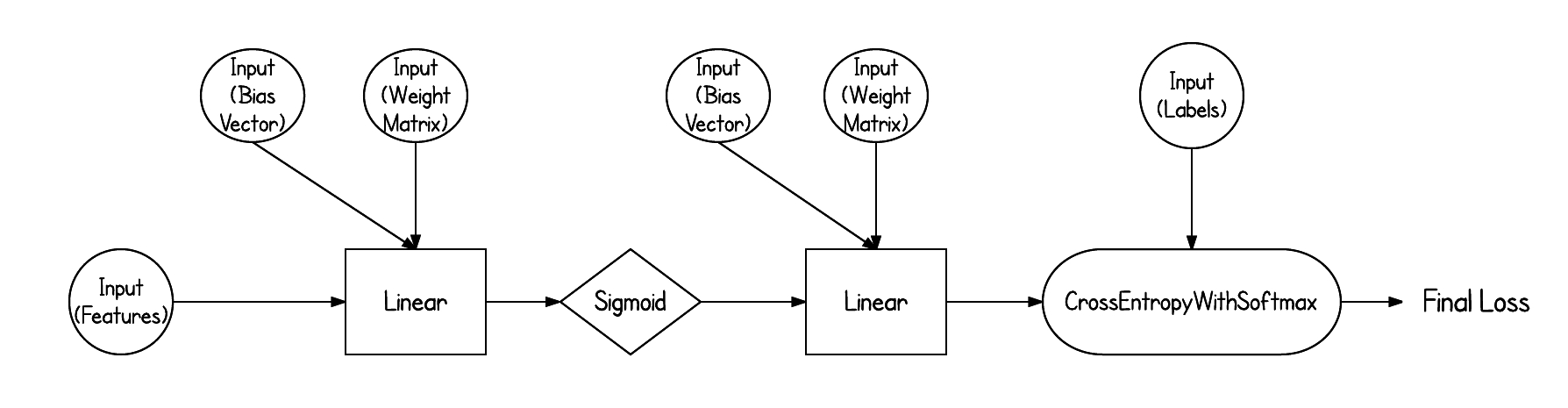 \n",
"\n",
"**USE [numpy](http://www.numpy.org/) FOR THE FOLLOWING EXERCISES**."
]
},
{
"cell_type": "markdown",
"metadata": {},
"source": [
"### Exercise - Implement `Linear` Node\n",
"\n",
"These are the shapes:\n",
"\n",
"* $X$ is $m$ by $n$\n",
"* $Z$ is $n$ by $p$\n",
"* $b$ has $p$ elements (row vector)\n",
"* $Z$ is $m$ by $p$\n",
"\n",
"In this exercise we'll implement the `Linear` node. This corresponds to the following function:\n",
"\n",
"$$\n",
"Z = f(X, W, b) = XW + b\n",
"$$\n",
"\n",
"\n",
"\n",
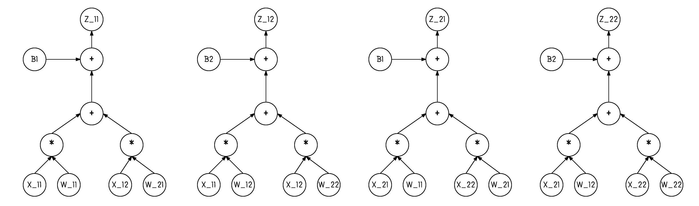
"or more explicitly, $Z$ being the output of $f(X, W, b)$:\n",
"\n",
"$$\n",
"Z_{ij} = \\sum_{k=1}^n X_{ik}W_{kj} + b_j\n",
"$$\n",
"\n",
"The latter format is very helpful when computing the derivatives. Computing the derivative of a matrix or vector can be intimidating since the computations are much more complex. But, as we've seen, if we're working with scalars the derivatives can be quite simple. The cool thing is computations with matrices and vectors are really just a lot of scalar computations!\n",
"\n",
"Let's walk through an example to walk sure we understand this computation.\n",
"\n",
"\n",
"$$\n",
"X = \\left[ \\begin{array}{cc}\n",
"-1 & -2 \\\\\n",
"-1 & -2\n",
"\\end{array} \\right]\n",
"\\hspace{0.3in}\n",
"%\n",
"W = \\left[ \\begin{array}{cc}\n",
"2 & -3 \\\\\n",
"2 & -3\n",
"\\end{array} \\right]\n",
"\\hspace{0.3in}\n",
"%\n",
"b = \\left[ \\begin{array}{cc}\n",
"-3 & -5\n",
"\\end{array} \\right]\n",
"\\hspace{0.3in}\n",
"%\n",
"Z = \\left[ \\begin{array}{cc}\n",
"? & ? \\\\\n",
"? & ?\n",
"\\end{array} \\right]\n",
"$$\n",
"\n",
"So if we want to compute $Z_{11}$ then the equation comes:\n",
"\n",
"$$\n",
"Z_{11} = \n",
"X_{11}W_{11} + X_{12}W_{21} + b_1 = \n",
"-1 * 2 + -2 * 2 + -3 = \n",
"-9\n",
"$$\n",
"\n",
"\n",
"To start out, try to work through these partials:\n",
"\n",
"$$\n",
"\\frac {\\partial Z_{ij}} {\\partial X_{ik}}\n",
"\\hspace{0.5in}\n",
"\\frac {\\partial Z_{ij}} {\\partial W_{kj}}\n",
"\\hspace{0.5in}\n",
"\\frac {\\partial Z_{ij}} {\\partial b_{j}}\n",
"$$\n",
"\n",
"Once you have those down see if you can make any generalizations. \n",
"\n",
"Additionally, it may be helpful to visualize the computation. Any duplicates $X, W, b$ nodes are just to make the visual easier, think of these duplicates as one and the same.\n",
"\n",
"
\n",
"\n",
"**USE [numpy](http://www.numpy.org/) FOR THE FOLLOWING EXERCISES**."
]
},
{
"cell_type": "markdown",
"metadata": {},
"source": [
"### Exercise - Implement `Linear` Node\n",
"\n",
"These are the shapes:\n",
"\n",
"* $X$ is $m$ by $n$\n",
"* $Z$ is $n$ by $p$\n",
"* $b$ has $p$ elements (row vector)\n",
"* $Z$ is $m$ by $p$\n",
"\n",
"In this exercise we'll implement the `Linear` node. This corresponds to the following function:\n",
"\n",
"$$\n",
"Z = f(X, W, b) = XW + b\n",
"$$\n",
"\n",
"\n",
"\n",
"or more explicitly, $Z$ being the output of $f(X, W, b)$:\n",
"\n",
"$$\n",
"Z_{ij} = \\sum_{k=1}^n X_{ik}W_{kj} + b_j\n",
"$$\n",
"\n",
"The latter format is very helpful when computing the derivatives. Computing the derivative of a matrix or vector can be intimidating since the computations are much more complex. But, as we've seen, if we're working with scalars the derivatives can be quite simple. The cool thing is computations with matrices and vectors are really just a lot of scalar computations!\n",
"\n",
"Let's walk through an example to walk sure we understand this computation.\n",
"\n",
"\n",
"$$\n",
"X = \\left[ \\begin{array}{cc}\n",
"-1 & -2 \\\\\n",
"-1 & -2\n",
"\\end{array} \\right]\n",
"\\hspace{0.3in}\n",
"%\n",
"W = \\left[ \\begin{array}{cc}\n",
"2 & -3 \\\\\n",
"2 & -3\n",
"\\end{array} \\right]\n",
"\\hspace{0.3in}\n",
"%\n",
"b = \\left[ \\begin{array}{cc}\n",
"-3 & -5\n",
"\\end{array} \\right]\n",
"\\hspace{0.3in}\n",
"%\n",
"Z = \\left[ \\begin{array}{cc}\n",
"? & ? \\\\\n",
"? & ?\n",
"\\end{array} \\right]\n",
"$$\n",
"\n",
"So if we want to compute $Z_{11}$ then the equation comes:\n",
"\n",
"$$\n",
"Z_{11} = \n",
"X_{11}W_{11} + X_{12}W_{21} + b_1 = \n",
"-1 * 2 + -2 * 2 + -3 = \n",
"-9\n",
"$$\n",
"\n",
"\n",
"To start out, try to work through these partials:\n",
"\n",
"$$\n",
"\\frac {\\partial Z_{ij}} {\\partial X_{ik}}\n",
"\\hspace{0.5in}\n",
"\\frac {\\partial Z_{ij}} {\\partial W_{kj}}\n",
"\\hspace{0.5in}\n",
"\\frac {\\partial Z_{ij}} {\\partial b_{j}}\n",
"$$\n",
"\n",
"Once you have those down see if you can make any generalizations. \n",
"\n",
"Additionally, it may be helpful to visualize the computation. Any duplicates $X, W, b$ nodes are just to make the visual easier, think of these duplicates as one and the same.\n",
"\n",
" \n",
"\n",
"We'll now visualize the gradient of the loss with respect to $X_{11}$. We remove the parts of the above image that don't contribute to the gradient. There are two paths back to $X_{11}$ from $Z$. How does the number of paths change as we change the matrix sizes?\n",
"\n",
"
\n",
"\n",
"We'll now visualize the gradient of the loss with respect to $X_{11}$. We remove the parts of the above image that don't contribute to the gradient. There are two paths back to $X_{11}$ from $Z$. How does the number of paths change as we change the matrix sizes?\n",
"\n",
"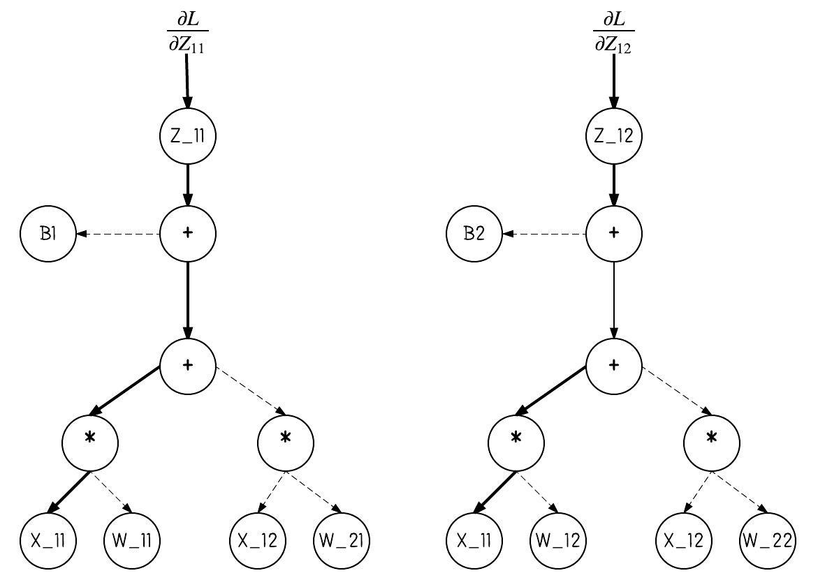 \n",
"\n",
"\n",
"\n",
"**HINT**: The `numpy.dot` function can be used to multiply matrices"
]
},
{
"cell_type": "code",
"execution_count": null,
"metadata": {
"collapsed": false
},
"outputs": [],
"source": [
"# RUN THIS BLOCK TO SEE IF YOUR CODE WORKS PROPERLY\n",
"\n",
"x_in, w_in, b_in = Input(), Input(), Input()\n",
"\n",
"# TODO: implement Linear in miniflow.py\n",
"f = Linear(x_in, w_in, b_in)\n",
"dummy = DummyGrad(f)\n",
"\n",
"x = np.array([[-1., -2.], [-1, -2]])\n",
"w = np.array([[2., -3], [2., -3]])\n",
"b = np.array([-3., -5])\n",
"dummy_grad = np.array([[1., 2.], [3, 4]])\n",
"\n",
"feed_dict = {x_in: x, w_in: w, b_in: b, dummy: dummy_grad}\n",
"loss, grads = value_and_grad(dummy, feed_dict, (x_in, w_in, b_in))\n",
"\n",
"# print(loss, grads)\n",
"assert np.allclose(loss, np.array([[-9., 4.], [-9., 4.]]))\n",
"assert np.allclose(grads[0], np.array([[-4., -4.], [-6., -6.]]))\n",
"assert np.allclose(grads[1], np.array([[-4., -6.], [-8., -12.]]))\n",
"assert np.allclose(grads[2], np.array([[4., 6.]]))"
]
},
{
"cell_type": "markdown",
"metadata": {},
"source": [
"### Exercise - Implement `Sigmoid` Node\n",
"\n",
"In this exercise we'll implement the `Sigmoid` node. This corresponds to the [sigmoid](https://en.wikipedia.org/wiki/Sigmoid_function) function:\n",
"\n",
"$$\n",
"sigmoid(x) = \\frac {1} {1 + exp(-x)}\n",
"$$\n",
"\n",
"What's the output if `x` is a scalar? A vector? A matrix?\n",
"\n",
"**Hint**: The `numpy.exp` function may be helpful (wink, wink)"
]
},
{
"cell_type": "code",
"execution_count": null,
"metadata": {
"collapsed": false
},
"outputs": [],
"source": [
"# RUN THIS BLOCK TO SEE IF YOUR CODE WORKS PROPERLY\n",
"\n",
"x_in = Input()\n",
"\n",
"# TODO: implement Sigmoid in miniflow.py\n",
"f = Sigmoid(x_in)\n",
"dummy = DummyGrad(f)\n",
"\n",
"x = np.array([-10., 0, 10])\n",
"\n",
"feed_dict = {x_in: x, dummy: 0.5}\n",
"loss, grads = value_and_grad(dummy, feed_dict, [x_in])\n",
"\n",
"# print(loss, grads)\n",
"assert np.allclose(loss, np.array([0., 0.5, 1.]), atol=1.e-4)\n",
"assert np.allclose(grads, np.array([0., 0.125, 0.]), atol=1.e-4)"
]
},
{
"cell_type": "markdown",
"metadata": {},
"source": [
"### Exercise - Implement `CrossEntropyWithSoftmax` Node\n",
"\n",
"\n",
"In this exercise you'll implement the `CrossEntropyWithSoftmax` node. This corresponds to implementing the [softmax](https://en.wikipedia.org/wiki/Softmax_function) and [cross entropy](https://en.wikipedia.org/wiki/Cross_entropy) functions."
]
},
{
"cell_type": "markdown",
"metadata": {},
"source": [
"#### Softmax\n",
"\n",
"\n",
"\n",
"$$\n",
"softmax(x) = \\frac{e^{x_i}} {\\sum_j e^{x_j}}\n",
"$$\n",
"\n",
"The input to the softmax function is a vector and the output is a vector of normalized probabilities. The input could also be a matrix. In this case each row/example should be treated in isolation. Output in this case would be a matrix of the same shape.\n",
"\n",
"Example:\n",
"\n",
"```\n",
"x = [0.2, 1.0, 0.3]\n",
"softmax(x) # [0.2309, 0.5138, 0.2551], sum over columns is 1.\n",
"```\n"
]
},
{
"cell_type": "markdown",
"metadata": {},
"source": [
"The `numpy.sum` function will be helpful for implementing both softmax and cross entropy loss, here's how it works."
]
},
{
"cell_type": "code",
"execution_count": null,
"metadata": {
"collapsed": false
},
"outputs": [],
"source": [
"# RUN THIS BLOCK TO SEE IF YOUR CODE WORKS PROPERLY\n",
"\n",
"import numpy as np\n",
"X = np.random.randn(3,5)\n",
"\n",
"# lose the dimension we sum across\n",
"# sum across rows\n",
"print(np.sum(X, axis=0, keepdims=False).shape)\n",
"# sum across columns\n",
"print(np.sum(X, axis=1, keepdims=False).shape)\n",
"\n",
"# keep the same number of dimensions\n",
"print(np.sum(X, axis=0, keepdims=True).shape)\n",
"print(np.sum(X, axis=1, keepdims=True).shape)"
]
},
{
"cell_type": "markdown",
"metadata": {},
"source": [
"As a sanity check when implementing softmax, you could check that summing over the columns adds up to 1 for each row. It should since the output of a softmax is a probability distribution over the classes."
]
},
{
"cell_type": "markdown",
"metadata": {},
"source": [
"#### Cross Entropy Loss\n",
"\n",
"Before we dive into the math behind the cross entropy loss (CE) let's get an intuition for how it helps our neural network perform better. Let's first think about what the inputs to CE are:\n",
"\n",
"1. The probabilities computed from the softmax activation (what we think the output is)\n",
"2. The labels (what the output actually is)\n",
"\n",
"What are we doing with these inputs?\n",
"\n",
"Fundamentally, we're comparing them, checking how different or similar they are. We want the output of the softmax to be as similar to the label as possible. If this is the case our loss will be low, if not it will be higher. Either way backpropagation will make the appropriate adjustments.\n",
"\n",
"At this point it still may not be clear what is actually being compared. So what is being compared?\n",
"\n",
"Probability distributions! More precisely [categorical distributions](https://en.wikipedia.org/wiki/Categorical_distribution), where the result can be one of $k$ possible outcomes. Remember the output from the softmax is a probability distribution (that's why it's important we make sure the values sum to 1). The label is a categorical distribution where $k-1$ values are 0 and one value is 1 (still adds up to 1). \n",
"\n",
"This might be strange, but, if I put an apple in front of you, would you say \"That's an apple 60% of the time, a banana 10% of the time, and 30% of the time a pineapple\". I hope not! You would be 100% certain that's an apple, after all, it can only be one of those things. The former though, may be the softmax output the neural network. In that case the CE would be computed by comparing these two vectors $[0.6, 0.10, 0.30]$ and $[1, 0, 0]$. As the neural network is trained the first vector will look more and more like the second. Alright, time for some math.\n",
"\n",
"$$\n",
"cross\\_entropy\\_loss = \\frac {1} {n} -\\sum_x P(x) * log(Q(x))\n",
"$$\n",
"\n",
"$P$ is the true distribution (labels) and $Q$ is the distribution of the neural network softmax. We sum over all the data, $x$ is an individual example, $n$ the number of examples. Let's walk through the example above.\n"
]
},
{
"cell_type": "code",
"execution_count": null,
"metadata": {
"collapsed": false
},
"outputs": [],
"source": [
"# 60% apple, 10% banana, 25% pineapple ... (crazy or maybe quantum world)\n",
"Qx = np.array([0.6, 0.1, 0.30]) \n",
"# 100% apple\n",
"Px = np.array([1., 0, 0])\n",
"log_Qx = np.log(Qx)\n",
"print(log_Qx)\n",
"loss = -np.sum(Px * log_Qx)\n",
"print(loss) # only the value multiplied by 1 effects the loss!\n",
"\n",
"# TODO: repeat this below\n",
"# we could simplify this to\n",
"-log_Qx[0] # 0 is the index where Px is 1\n",
"\n",
"# Feel free to play around with Qx and Px to get a feel for the loss."
]
},
{
"cell_type": "markdown",
"metadata": {},
"source": [
"You'll implement the latter version, where we just index `log_Qx`. This allows us to represent the label as just 1 number $[0, k-1]$, rather than a vector of $k$ numbers.\n",
"\n",
"Here's the math version:\n",
"\n",
"* $X$ is a matrix from the output of a softmax activation. Each row is a categorical distribution.\n",
"* $y$ is a vector of labels $[0, k-1]$, $k$ being the number of classes.\n",
"* $n$ is the number of rows of $X$.\n",
"\n",
"$$\n",
"cross\\_entropy\\_loss(X, y) = \\frac {1} {n} \\sum_{i=1}^n - log(X_{i{y_i}})\n",
"$$\n",
"\n",
"Ok, but how will this loss encourage our model to classify correctly?\n",
"\n",
"There are 2 key pieces of information here:\n",
"\n",
"1. $probs$ contains values between 0 and 1\n",
"2. $log(0) = -inf$ and $log(1) = 0$; the possible log values are either negative or 0.\n",
"\n",
"Clearly we'd like the probability of the index of the correct label to be 1 or close to it and if it's close to 0 we'll be heavily penalized and our will loss to shoot up. Note the negative sign sets the problem up nicely for minimizing the loss.\n",
"\n",
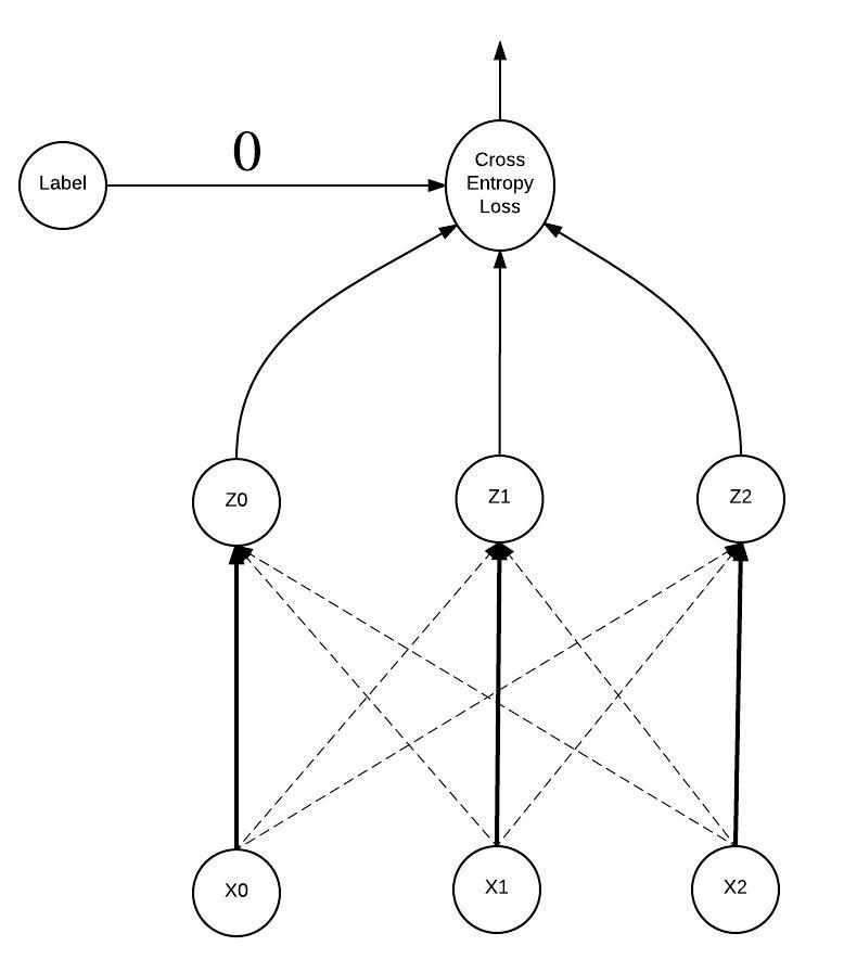
"Let's look at some visuals, we're going to stay with the fruit classifier example above. In the following graphs the $x$ values are the input to the softmax function, $z$ values the output of the softmax function which are fed into the cross entropy loss function. So $z_0 = 0.6$, $z_1 = 0.1$, and $z_2 = 0.3$. The label distribution is $[1, 0, 0]$ but remember we can simplify this to just use the index where the probability is 1, so our label is 0. \n",
"\n",
"#### Softmax + Cross Entropy Forward Pass\n",
"\n",
"Notice each $x_i$ is connected to each $z_i$, this is because each $x_i$ plays a role in computing each $z_i$. Hmmm, that's a lot to keep track of for the backward pass.\n",
"\n",
"
\n",
"\n",
"\n",
"\n",
"**HINT**: The `numpy.dot` function can be used to multiply matrices"
]
},
{
"cell_type": "code",
"execution_count": null,
"metadata": {
"collapsed": false
},
"outputs": [],
"source": [
"# RUN THIS BLOCK TO SEE IF YOUR CODE WORKS PROPERLY\n",
"\n",
"x_in, w_in, b_in = Input(), Input(), Input()\n",
"\n",
"# TODO: implement Linear in miniflow.py\n",
"f = Linear(x_in, w_in, b_in)\n",
"dummy = DummyGrad(f)\n",
"\n",
"x = np.array([[-1., -2.], [-1, -2]])\n",
"w = np.array([[2., -3], [2., -3]])\n",
"b = np.array([-3., -5])\n",
"dummy_grad = np.array([[1., 2.], [3, 4]])\n",
"\n",
"feed_dict = {x_in: x, w_in: w, b_in: b, dummy: dummy_grad}\n",
"loss, grads = value_and_grad(dummy, feed_dict, (x_in, w_in, b_in))\n",
"\n",
"# print(loss, grads)\n",
"assert np.allclose(loss, np.array([[-9., 4.], [-9., 4.]]))\n",
"assert np.allclose(grads[0], np.array([[-4., -4.], [-6., -6.]]))\n",
"assert np.allclose(grads[1], np.array([[-4., -6.], [-8., -12.]]))\n",
"assert np.allclose(grads[2], np.array([[4., 6.]]))"
]
},
{
"cell_type": "markdown",
"metadata": {},
"source": [
"### Exercise - Implement `Sigmoid` Node\n",
"\n",
"In this exercise we'll implement the `Sigmoid` node. This corresponds to the [sigmoid](https://en.wikipedia.org/wiki/Sigmoid_function) function:\n",
"\n",
"$$\n",
"sigmoid(x) = \\frac {1} {1 + exp(-x)}\n",
"$$\n",
"\n",
"What's the output if `x` is a scalar? A vector? A matrix?\n",
"\n",
"**Hint**: The `numpy.exp` function may be helpful (wink, wink)"
]
},
{
"cell_type": "code",
"execution_count": null,
"metadata": {
"collapsed": false
},
"outputs": [],
"source": [
"# RUN THIS BLOCK TO SEE IF YOUR CODE WORKS PROPERLY\n",
"\n",
"x_in = Input()\n",
"\n",
"# TODO: implement Sigmoid in miniflow.py\n",
"f = Sigmoid(x_in)\n",
"dummy = DummyGrad(f)\n",
"\n",
"x = np.array([-10., 0, 10])\n",
"\n",
"feed_dict = {x_in: x, dummy: 0.5}\n",
"loss, grads = value_and_grad(dummy, feed_dict, [x_in])\n",
"\n",
"# print(loss, grads)\n",
"assert np.allclose(loss, np.array([0., 0.5, 1.]), atol=1.e-4)\n",
"assert np.allclose(grads, np.array([0., 0.125, 0.]), atol=1.e-4)"
]
},
{
"cell_type": "markdown",
"metadata": {},
"source": [
"### Exercise - Implement `CrossEntropyWithSoftmax` Node\n",
"\n",
"\n",
"In this exercise you'll implement the `CrossEntropyWithSoftmax` node. This corresponds to implementing the [softmax](https://en.wikipedia.org/wiki/Softmax_function) and [cross entropy](https://en.wikipedia.org/wiki/Cross_entropy) functions."
]
},
{
"cell_type": "markdown",
"metadata": {},
"source": [
"#### Softmax\n",
"\n",
"\n",
"\n",
"$$\n",
"softmax(x) = \\frac{e^{x_i}} {\\sum_j e^{x_j}}\n",
"$$\n",
"\n",
"The input to the softmax function is a vector and the output is a vector of normalized probabilities. The input could also be a matrix. In this case each row/example should be treated in isolation. Output in this case would be a matrix of the same shape.\n",
"\n",
"Example:\n",
"\n",
"```\n",
"x = [0.2, 1.0, 0.3]\n",
"softmax(x) # [0.2309, 0.5138, 0.2551], sum over columns is 1.\n",
"```\n"
]
},
{
"cell_type": "markdown",
"metadata": {},
"source": [
"The `numpy.sum` function will be helpful for implementing both softmax and cross entropy loss, here's how it works."
]
},
{
"cell_type": "code",
"execution_count": null,
"metadata": {
"collapsed": false
},
"outputs": [],
"source": [
"# RUN THIS BLOCK TO SEE IF YOUR CODE WORKS PROPERLY\n",
"\n",
"import numpy as np\n",
"X = np.random.randn(3,5)\n",
"\n",
"# lose the dimension we sum across\n",
"# sum across rows\n",
"print(np.sum(X, axis=0, keepdims=False).shape)\n",
"# sum across columns\n",
"print(np.sum(X, axis=1, keepdims=False).shape)\n",
"\n",
"# keep the same number of dimensions\n",
"print(np.sum(X, axis=0, keepdims=True).shape)\n",
"print(np.sum(X, axis=1, keepdims=True).shape)"
]
},
{
"cell_type": "markdown",
"metadata": {},
"source": [
"As a sanity check when implementing softmax, you could check that summing over the columns adds up to 1 for each row. It should since the output of a softmax is a probability distribution over the classes."
]
},
{
"cell_type": "markdown",
"metadata": {},
"source": [
"#### Cross Entropy Loss\n",
"\n",
"Before we dive into the math behind the cross entropy loss (CE) let's get an intuition for how it helps our neural network perform better. Let's first think about what the inputs to CE are:\n",
"\n",
"1. The probabilities computed from the softmax activation (what we think the output is)\n",
"2. The labels (what the output actually is)\n",
"\n",
"What are we doing with these inputs?\n",
"\n",
"Fundamentally, we're comparing them, checking how different or similar they are. We want the output of the softmax to be as similar to the label as possible. If this is the case our loss will be low, if not it will be higher. Either way backpropagation will make the appropriate adjustments.\n",
"\n",
"At this point it still may not be clear what is actually being compared. So what is being compared?\n",
"\n",
"Probability distributions! More precisely [categorical distributions](https://en.wikipedia.org/wiki/Categorical_distribution), where the result can be one of $k$ possible outcomes. Remember the output from the softmax is a probability distribution (that's why it's important we make sure the values sum to 1). The label is a categorical distribution where $k-1$ values are 0 and one value is 1 (still adds up to 1). \n",
"\n",
"This might be strange, but, if I put an apple in front of you, would you say \"That's an apple 60% of the time, a banana 10% of the time, and 30% of the time a pineapple\". I hope not! You would be 100% certain that's an apple, after all, it can only be one of those things. The former though, may be the softmax output the neural network. In that case the CE would be computed by comparing these two vectors $[0.6, 0.10, 0.30]$ and $[1, 0, 0]$. As the neural network is trained the first vector will look more and more like the second. Alright, time for some math.\n",
"\n",
"$$\n",
"cross\\_entropy\\_loss = \\frac {1} {n} -\\sum_x P(x) * log(Q(x))\n",
"$$\n",
"\n",
"$P$ is the true distribution (labels) and $Q$ is the distribution of the neural network softmax. We sum over all the data, $x$ is an individual example, $n$ the number of examples. Let's walk through the example above.\n"
]
},
{
"cell_type": "code",
"execution_count": null,
"metadata": {
"collapsed": false
},
"outputs": [],
"source": [
"# 60% apple, 10% banana, 25% pineapple ... (crazy or maybe quantum world)\n",
"Qx = np.array([0.6, 0.1, 0.30]) \n",
"# 100% apple\n",
"Px = np.array([1., 0, 0])\n",
"log_Qx = np.log(Qx)\n",
"print(log_Qx)\n",
"loss = -np.sum(Px * log_Qx)\n",
"print(loss) # only the value multiplied by 1 effects the loss!\n",
"\n",
"# TODO: repeat this below\n",
"# we could simplify this to\n",
"-log_Qx[0] # 0 is the index where Px is 1\n",
"\n",
"# Feel free to play around with Qx and Px to get a feel for the loss."
]
},
{
"cell_type": "markdown",
"metadata": {},
"source": [
"You'll implement the latter version, where we just index `log_Qx`. This allows us to represent the label as just 1 number $[0, k-1]$, rather than a vector of $k$ numbers.\n",
"\n",
"Here's the math version:\n",
"\n",
"* $X$ is a matrix from the output of a softmax activation. Each row is a categorical distribution.\n",
"* $y$ is a vector of labels $[0, k-1]$, $k$ being the number of classes.\n",
"* $n$ is the number of rows of $X$.\n",
"\n",
"$$\n",
"cross\\_entropy\\_loss(X, y) = \\frac {1} {n} \\sum_{i=1}^n - log(X_{i{y_i}})\n",
"$$\n",
"\n",
"Ok, but how will this loss encourage our model to classify correctly?\n",
"\n",
"There are 2 key pieces of information here:\n",
"\n",
"1. $probs$ contains values between 0 and 1\n",
"2. $log(0) = -inf$ and $log(1) = 0$; the possible log values are either negative or 0.\n",
"\n",
"Clearly we'd like the probability of the index of the correct label to be 1 or close to it and if it's close to 0 we'll be heavily penalized and our will loss to shoot up. Note the negative sign sets the problem up nicely for minimizing the loss.\n",
"\n",
"Let's look at some visuals, we're going to stay with the fruit classifier example above. In the following graphs the $x$ values are the input to the softmax function, $z$ values the output of the softmax function which are fed into the cross entropy loss function. So $z_0 = 0.6$, $z_1 = 0.1$, and $z_2 = 0.3$. The label distribution is $[1, 0, 0]$ but remember we can simplify this to just use the index where the probability is 1, so our label is 0. \n",
"\n",
"#### Softmax + Cross Entropy Forward Pass\n",
"\n",
"Notice each $x_i$ is connected to each $z_i$, this is because each $x_i$ plays a role in computing each $z_i$. Hmmm, that's a lot to keep track of for the backward pass.\n",
"\n",
" \n",
"\n",
"#### Softmax + Cross Entropy Backward Pass\n",
"\n",
"Remember back when we discovered only one value from the softmax output will effect the loss? Here we see the consequences of that. The only derivative that is not 0, is the derivative of the value that effected the loss, in this case the label was 0 so it corresponds to the $z_0$ node. In addition, we no longer have to consider the gradient of any softmax output node besides $z_0$, this greatly simplifies $\\frac {\\partial L}{\\partial x_i}$!\n",
"\n",
"
\n",
"\n",
"#### Softmax + Cross Entropy Backward Pass\n",
"\n",
"Remember back when we discovered only one value from the softmax output will effect the loss? Here we see the consequences of that. The only derivative that is not 0, is the derivative of the value that effected the loss, in this case the label was 0 so it corresponds to the $z_0$ node. In addition, we no longer have to consider the gradient of any softmax output node besides $z_0$, this greatly simplifies $\\frac {\\partial L}{\\partial x_i}$!\n",
"\n",
"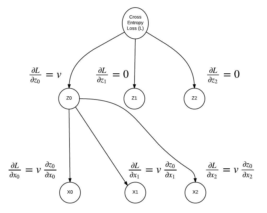 "
]
},
{
"cell_type": "code",
"execution_count": null,
"metadata": {
"collapsed": false
},
"outputs": [],
"source": [
"# RUN THIS BLOCK TO SEE IF YOUR CODE WORKS PROPERLY\n",
"\n",
"x_in = Input()\n",
"y_in = Input()\n",
"\n",
"# TODO: implement CrossEntropyWithSoftmax in miniflow.py\n",
"# No DummyGrad this time! Guaranteed to be last node in our graph.\n",
"f = CrossEntropyWithSoftmax(x_in, y_in)\n",
"\n",
"# values to feed input nodes\n",
"x = np.array([[0.5, 1., 1.5]])\n",
"# in this example we have a choice 3 classes (x has 3 columns)\n",
"# so our label can one of 0,1,2. It's 1 in this case.\n",
"y = np.array([1])\n",
"\n",
"feed_dict = {x_in: x, y_in: y}\n",
"loss, grads = value_and_grad(f, feed_dict, wrt=[x_in])\n",
"\n",
"# print(loss, grads)\n",
"\n",
"# Look at the expected value of softmax(x) and the expected value of the gradient with\n",
"# respect to x\n",
"assert np.allclose(f._softmax(x), [[0.1863, 0.3072, 0.5064]], atol=1.e-4)\n",
"assert np.allclose(loss, 1.1802, atol=1.e-4)\n",
"assert np.allclose(grads, np.array([[0.1863, -0.6928, 0.5064]]), atol=1.e-4)"
]
},
{
"cell_type": "markdown",
"metadata": {},
"source": [
"## Stochastic Gradient Descent (SGD)\n",
"\n",
"At this point you should have all the nodes implemented and working correctly. Computing those weight gradients is a breeze! Now that we have the gradients what do we do with them?\n",
"\n",
"As it turns out the gradient is analogous to the **steepest ascent direction**. Let's imagine that we are our neural network and we're in a park - not just any park though, a hilly park. We also know that we perform our best when we're on the highest hill, so let's go there! \n",
"\n",
"There are a couple of issues though ... we are:\n",
"\n",
"1. Blindfolded\n",
"2. Dropped randomly somewhere in the park (random weights!). We'd be hard pressed to find the highest hill in our current condition.\n",
"\n",
"Luckily for us, we have a talking bird by our side. Her name is Gradient and she's very good at informing us which direction causes us to ascend the hill the fastest. Unfortunately for Gradient, her vision isn't the greatest and she can only see the local area. It might be the case we get to the top of a hill, but not the highest one.\n",
"\n",
"
"
]
},
{
"cell_type": "code",
"execution_count": null,
"metadata": {
"collapsed": false
},
"outputs": [],
"source": [
"# RUN THIS BLOCK TO SEE IF YOUR CODE WORKS PROPERLY\n",
"\n",
"x_in = Input()\n",
"y_in = Input()\n",
"\n",
"# TODO: implement CrossEntropyWithSoftmax in miniflow.py\n",
"# No DummyGrad this time! Guaranteed to be last node in our graph.\n",
"f = CrossEntropyWithSoftmax(x_in, y_in)\n",
"\n",
"# values to feed input nodes\n",
"x = np.array([[0.5, 1., 1.5]])\n",
"# in this example we have a choice 3 classes (x has 3 columns)\n",
"# so our label can one of 0,1,2. It's 1 in this case.\n",
"y = np.array([1])\n",
"\n",
"feed_dict = {x_in: x, y_in: y}\n",
"loss, grads = value_and_grad(f, feed_dict, wrt=[x_in])\n",
"\n",
"# print(loss, grads)\n",
"\n",
"# Look at the expected value of softmax(x) and the expected value of the gradient with\n",
"# respect to x\n",
"assert np.allclose(f._softmax(x), [[0.1863, 0.3072, 0.5064]], atol=1.e-4)\n",
"assert np.allclose(loss, 1.1802, atol=1.e-4)\n",
"assert np.allclose(grads, np.array([[0.1863, -0.6928, 0.5064]]), atol=1.e-4)"
]
},
{
"cell_type": "markdown",
"metadata": {},
"source": [
"## Stochastic Gradient Descent (SGD)\n",
"\n",
"At this point you should have all the nodes implemented and working correctly. Computing those weight gradients is a breeze! Now that we have the gradients what do we do with them?\n",
"\n",
"As it turns out the gradient is analogous to the **steepest ascent direction**. Let's imagine that we are our neural network and we're in a park - not just any park though, a hilly park. We also know that we perform our best when we're on the highest hill, so let's go there! \n",
"\n",
"There are a couple of issues though ... we are:\n",
"\n",
"1. Blindfolded\n",
"2. Dropped randomly somewhere in the park (random weights!). We'd be hard pressed to find the highest hill in our current condition.\n",
"\n",
"Luckily for us, we have a talking bird by our side. Her name is Gradient and she's very good at informing us which direction causes us to ascend the hill the fastest. Unfortunately for Gradient, her vision isn't the greatest and she can only see the local area. It might be the case we get to the top of a hill, but not the highest one.\n",
"\n",
" \n",
"\n",
"Typically we're minimizing a function, not maximizing. The above analogy still holds, we're just descending instead of ascending (searching for lowest valley vs. highest hill). Making this adjustment is very simple, just put a negative sign on the gradient.\n",
"\n",
"There's one more thing to think about, we know what direction to step in but how large of a step should we take? Too small a step and it could take a very long time to converge, and too large a step could overshoot the target cause divergence. In practice the most common step sizes are 1e-3 and 1e-4, sometimes 1e-2 and 1e-1 work well too. Note: the *step size* is more commonly known as the *learning rate*.\n",
"\n",
"Here's roughly what SGD looks like with miniflow.\n",
"\n",
"```\n",
"f = ... # output node\n",
"wrt = [...] # weight input nodes\n",
"W = ... # weight for Linear node\n",
"b = ... # bias for Linear node\n",
"while True:\n",
" feed_dict = {...} # new batch of data\n",
" loss, grad = value_and_grad(f, feed_dict, wrt)\n",
" # get the grad for W and b\n",
" dW = grad[...]\n",
" db = grad[...] \n",
" # descending in the direction of the gradient\n",
" W[:] -= step_size * dW\n",
" b[:] -= step_size * db\n",
" \n",
"```"
]
},
{
"cell_type": "markdown",
"metadata": {},
"source": [
"### Exercise: Train a neural net on MNIST with SGD\n",
"\n",
"You now have all the pieces in place, all that's left to do is fit them together like legos.\n",
"\n",
"TODO: lego picture\n",
"\n",
"Your task is now to classify handwritten digits from the MNIST dataset."
]
},
{
"cell_type": "code",
"execution_count": null,
"metadata": {
"collapsed": false
},
"outputs": [],
"source": [
"# load MNIST\n",
"from tensorflow.examples.tutorials.mnist import input_data\n",
"mnist = input_data.read_data_sets(\"MNIST_data/\", one_hot=False)"
]
},
{
"cell_type": "code",
"execution_count": null,
"metadata": {
"collapsed": false
},
"outputs": [],
"source": [
"# getting input and label data\n",
"X_batch, y_batch = mnist.train.next_batch(128)\n",
"print(X_batch.shape, y_batch.shape)"
]
},
{
"cell_type": "code",
"execution_count": null,
"metadata": {
"collapsed": false
},
"outputs": [],
"source": [
"X_val = mnist.validation.images\n",
"y_val = mnist.validation.labels.astype(np.int8)\n",
"X_test = mnist.test.images\n",
"y_test = mnist.test.labels.astype(np.int8)"
]
},
{
"cell_type": "markdown",
"metadata": {},
"source": [
"### Exercise: Train a neural net on MNIST with SGD\n",
"\n",
"You should hit above 90% accuracy on even a 1-layer neural network."
]
},
{
"cell_type": "code",
"execution_count": null,
"metadata": {
"collapsed": true
},
"outputs": [],
"source": [
"# TODO: initialize weights\n",
"\n",
"# TODO: define architecture, you can use the architecture in the miniflow graph shown earlier"
]
},
{
"cell_type": "code",
"execution_count": null,
"metadata": {
"collapsed": false
},
"outputs": [],
"source": [
"# TODO: set step size and batch size\n",
"step_size = ...\n",
"batch_size = ...\n",
"\n",
"for i in range(10000):\n",
" X_batch, y_batch = mnist.train.next_batch(batch_size)\n",
" y_batch = y_batch.astype(np.int8)\n",
" \n",
" # TODO: get the loss and grad\n",
" loss, grad = value_and_grad(...)\n",
" \n",
" if i % 1000 == 0:\n",
" print(\"Iteration {}\".format(i))\n",
" print(\"Loss = {}\".format(loss))\n",
" \n",
" # TODO: get the accuracy of the validation dataset\n",
" # similar to value_and_grad except there's no wrt list\n",
" acc = accuracy(...)\n",
" \n",
" print(\"Validation Accuracy = {}\".format(acc))\n",
" print('----------------')\n",
" \n",
" # TODO: SGD updates with gradient\n",
" # SGD code goes here ...\n",
" \n",
" \n",
"# TODO: get the accuracy of the testing dataset\n",
"acc = accuracy(...)\n",
"\n",
"print('----------------')\n",
"print(\"Testing Accuracy = {}\".format(acc))"
]
},
{
"cell_type": "markdown",
"metadata": {},
"source": [
"## Outro to TensorFlow"
]
},
{
"cell_type": "markdown",
"metadata": {},
"source": [
"In this lab you created a library, miniflow, for computing differentiable graphs. Using miniflow, you created a neural network that can classify handwritten digits with high accuracy. Not too shabby! Hopefully you now have a solid grasp of differentiable graphs and backpropagation. \n",
"\n",
"You probably also noticed how tedious all this work can be! It would be nice if someone already had written all this code for us, made it really fast, usable on GPUs, mobile devices and had a gigantic ecosystem around it so we can be assured it'll just get better and better ... Oh wait! It's not a fantasy. \n",
"\n",
"All of that is true and it's called [Tensorflow](https://www.tensorflow.org/), developed by the fine folks at Google and now a thriving open source project! In the future you'll use TensorFlow, but you can always come back to miniflow if you've grown attached :-)"
]
}
],
"metadata": {
"anaconda-cloud": {},
"kernelspec": {
"display_name": "Python 3",
"language": "python",
"name": "python3"
},
"language_info": {
"codemirror_mode": {
"name": "ipython",
"version": 3
},
"file_extension": ".py",
"mimetype": "text/x-python",
"name": "python",
"nbconvert_exporter": "python",
"pygments_lexer": "ipython3",
"version": "3.5.2"
}
},
"nbformat": 4,
"nbformat_minor": 1
}
\n",
"\n",
"Typically we're minimizing a function, not maximizing. The above analogy still holds, we're just descending instead of ascending (searching for lowest valley vs. highest hill). Making this adjustment is very simple, just put a negative sign on the gradient.\n",
"\n",
"There's one more thing to think about, we know what direction to step in but how large of a step should we take? Too small a step and it could take a very long time to converge, and too large a step could overshoot the target cause divergence. In practice the most common step sizes are 1e-3 and 1e-4, sometimes 1e-2 and 1e-1 work well too. Note: the *step size* is more commonly known as the *learning rate*.\n",
"\n",
"Here's roughly what SGD looks like with miniflow.\n",
"\n",
"```\n",
"f = ... # output node\n",
"wrt = [...] # weight input nodes\n",
"W = ... # weight for Linear node\n",
"b = ... # bias for Linear node\n",
"while True:\n",
" feed_dict = {...} # new batch of data\n",
" loss, grad = value_and_grad(f, feed_dict, wrt)\n",
" # get the grad for W and b\n",
" dW = grad[...]\n",
" db = grad[...] \n",
" # descending in the direction of the gradient\n",
" W[:] -= step_size * dW\n",
" b[:] -= step_size * db\n",
" \n",
"```"
]
},
{
"cell_type": "markdown",
"metadata": {},
"source": [
"### Exercise: Train a neural net on MNIST with SGD\n",
"\n",
"You now have all the pieces in place, all that's left to do is fit them together like legos.\n",
"\n",
"TODO: lego picture\n",
"\n",
"Your task is now to classify handwritten digits from the MNIST dataset."
]
},
{
"cell_type": "code",
"execution_count": null,
"metadata": {
"collapsed": false
},
"outputs": [],
"source": [
"# load MNIST\n",
"from tensorflow.examples.tutorials.mnist import input_data\n",
"mnist = input_data.read_data_sets(\"MNIST_data/\", one_hot=False)"
]
},
{
"cell_type": "code",
"execution_count": null,
"metadata": {
"collapsed": false
},
"outputs": [],
"source": [
"# getting input and label data\n",
"X_batch, y_batch = mnist.train.next_batch(128)\n",
"print(X_batch.shape, y_batch.shape)"
]
},
{
"cell_type": "code",
"execution_count": null,
"metadata": {
"collapsed": false
},
"outputs": [],
"source": [
"X_val = mnist.validation.images\n",
"y_val = mnist.validation.labels.astype(np.int8)\n",
"X_test = mnist.test.images\n",
"y_test = mnist.test.labels.astype(np.int8)"
]
},
{
"cell_type": "markdown",
"metadata": {},
"source": [
"### Exercise: Train a neural net on MNIST with SGD\n",
"\n",
"You should hit above 90% accuracy on even a 1-layer neural network."
]
},
{
"cell_type": "code",
"execution_count": null,
"metadata": {
"collapsed": true
},
"outputs": [],
"source": [
"# TODO: initialize weights\n",
"\n",
"# TODO: define architecture, you can use the architecture in the miniflow graph shown earlier"
]
},
{
"cell_type": "code",
"execution_count": null,
"metadata": {
"collapsed": false
},
"outputs": [],
"source": [
"# TODO: set step size and batch size\n",
"step_size = ...\n",
"batch_size = ...\n",
"\n",
"for i in range(10000):\n",
" X_batch, y_batch = mnist.train.next_batch(batch_size)\n",
" y_batch = y_batch.astype(np.int8)\n",
" \n",
" # TODO: get the loss and grad\n",
" loss, grad = value_and_grad(...)\n",
" \n",
" if i % 1000 == 0:\n",
" print(\"Iteration {}\".format(i))\n",
" print(\"Loss = {}\".format(loss))\n",
" \n",
" # TODO: get the accuracy of the validation dataset\n",
" # similar to value_and_grad except there's no wrt list\n",
" acc = accuracy(...)\n",
" \n",
" print(\"Validation Accuracy = {}\".format(acc))\n",
" print('----------------')\n",
" \n",
" # TODO: SGD updates with gradient\n",
" # SGD code goes here ...\n",
" \n",
" \n",
"# TODO: get the accuracy of the testing dataset\n",
"acc = accuracy(...)\n",
"\n",
"print('----------------')\n",
"print(\"Testing Accuracy = {}\".format(acc))"
]
},
{
"cell_type": "markdown",
"metadata": {},
"source": [
"## Outro to TensorFlow"
]
},
{
"cell_type": "markdown",
"metadata": {},
"source": [
"In this lab you created a library, miniflow, for computing differentiable graphs. Using miniflow, you created a neural network that can classify handwritten digits with high accuracy. Not too shabby! Hopefully you now have a solid grasp of differentiable graphs and backpropagation. \n",
"\n",
"You probably also noticed how tedious all this work can be! It would be nice if someone already had written all this code for us, made it really fast, usable on GPUs, mobile devices and had a gigantic ecosystem around it so we can be assured it'll just get better and better ... Oh wait! It's not a fantasy. \n",
"\n",
"All of that is true and it's called [Tensorflow](https://www.tensorflow.org/), developed by the fine folks at Google and now a thriving open source project! In the future you'll use TensorFlow, but you can always come back to miniflow if you've grown attached :-)"
]
}
],
"metadata": {
"anaconda-cloud": {},
"kernelspec": {
"display_name": "Python 3",
"language": "python",
"name": "python3"
},
"language_info": {
"codemirror_mode": {
"name": "ipython",
"version": 3
},
"file_extension": ".py",
"mimetype": "text/x-python",
"name": "python",
"nbconvert_exporter": "python",
"pygments_lexer": "ipython3",
"version": "3.5.2"
}
},
"nbformat": 4,
"nbformat_minor": 1
}