{
"cells": [
{
"cell_type": "markdown",
"metadata": {},
"source": [
"# Frequency and the fast Fourier transform\n",
"\n",
"> If you want to find the secrets of the universe, think in terms of energy,\n",
"> frequency and vibration.\n",
">\n",
"> — Nikola Tesla\n",
"\n",
"*This chapter was written in collaboration with SW's father, PW van der Walt.*\n",
"\n",
"This chapter will depart slightly from the format of the rest of the\n",
"book. In particular, you may find the *code* in the chapter quite\n",
"modest. Instead, we want to illustrate an elegant *algorithm*, the\n",
"Fast Fourier Transform (FFT), that is endlessly useful, implemented in\n",
"SciPy, and works, of course, on NumPy arrays.\n",
"\n",
"## Introducing frequency\n",
"\n",
"We'll start by setting up some plotting styles and importing the usual\n",
"suspects:"
]
},
{
"cell_type": "code",
"execution_count": null,
"metadata": {},
"outputs": [],
"source": [
"# Make plots appear inline, set custom plotting style\n",
"%matplotlib inline\n",
"import matplotlib.pyplot as plt\n",
"plt.style.use('style/elegant.mplstyle')"
]
},
{
"cell_type": "code",
"execution_count": null,
"metadata": {},
"outputs": [],
"source": [
"import numpy as np"
]
},
{
"cell_type": "markdown",
"metadata": {},
"source": [
"The discrete[^discrete] Fourier transform (DFT) is a mathematical technique\n",
"to convert temporal or spatial data into *frequency domain* data.\n",
"*Frequency* is a familiar concept, due to its colloquial occurrence in\n",
"the English language: the lowest notes your headphones can rumble out\n",
"are around 20 Hertz, whereas middle C on a piano lies around 261.6\n",
"Hertz. Hertz (Hz), or oscillations per second, in this case literally\n",
"refers to the number of times per second at which the membrane inside\n",
"the headphone moves to-and-fro. That, in turn, creates compressed\n",
"pulses of air which, upon arrival at your eardrum, induces a vibration\n",
"at the same frequency. So, if you take a simple periodic function, $\\sin(10 \\times 2 \\pi t)$, you can view it as a wave:"
]
},
{
"cell_type": "code",
"execution_count": null,
"metadata": {},
"outputs": [],
"source": [
"f = 10 # Frequency, in cycles per second, or Hertz\n",
"f_s = 100 # Sampling rate, or number of measurements per second\n",
"\n",
"t = np.linspace(0, 2, 2 * f_s, endpoint=False)\n",
"x = np.sin(f * 2 * np.pi * t)\n",
"\n",
"fig, ax = plt.subplots()\n",
"ax.plot(t, x)\n",
"ax.set_xlabel('Time [s]')\n",
"ax.set_ylabel('Signal amplitude');"
]
},
{
"cell_type": "markdown",
"metadata": {},
"source": [
"\n",
"\n",
"[^discrete]: The discrete Fourier transform operates on sampled data,\n",
" in contrast to the standard Fourier transform which is\n",
" defined for continuous functions.\n",
"\n",
"Or you can equivalently think of it as a repeating signal of\n",
"*frequency* 10 Hertz (it repeats once every $1/10$ seconds—a length of\n",
"time we call its *period*). Although we naturally associate frequency\n",
"with time, it can equally well be applied to space. E.g., a\n",
"photo of a textile patterns exhibits high *spatial frequency*, whereas\n",
"the sky or other smooth objects have low spatial frequency.\n",
"\n",
"Let us now examine our sinusoid through application of the discrete Fourier\n",
"transform:"
]
},
{
"cell_type": "code",
"execution_count": null,
"metadata": {},
"outputs": [],
"source": [
"from scipy import fftpack\n",
"\n",
"X = fftpack.fft(x)\n",
"freqs = fftpack.fftfreq(len(x)) * f_s\n",
"\n",
"fig, ax = plt.subplots()\n",
"\n",
"ax.stem(freqs, np.abs(X))\n",
"ax.set_xlabel('Frequency in Hertz [Hz]')\n",
"ax.set_ylabel('Frequency Domain (Spectrum) Magnitude')\n",
"ax.set_xlim(-f_s / 2, f_s / 2)\n",
"ax.set_ylim(-5, 110)"
]
},
{
"cell_type": "markdown",
"metadata": {},
"source": [
"\n",
"\n",
"We see that the output of the FFT is a one-dimensional array of the\n",
"same shape as the input, containing complex values. All values are\n",
"zero, except for two entries. Traditionally, we visualize the\n",
"magnitude of the result as a *stem plot*, in which the height of each\n",
"stem corresponds to the underlying value.\n",
"\n",
"(We explain why you see positive and negative frequencies later on\n",
"in the sidebox titled \"Discrete Fourier transforms\". You may also\n",
"refer to that section for a more in-depth overview of the underlying\n",
"mathematics.)\n",
"\n",
"The Fourier transform takes us from the *time* to the *frequency*\n",
"domain, and this turns out to have a massive number of applications.\n",
"The *fast Fourier transform* is an algorithm for computing the\n",
"discrete Fourier transform; it achieves its high speed by storing and\n",
"re-using results of computations as it progresses.\n",
"\n",
"In this chapter, we examine a few applications of the discrete Fourier\n",
"transform to demonstrate that the FFT can be applied to\n",
"multidimensional data (not just 1D measurements) to achieve a variety\n",
"of goals.\n",
"\n",
"## Illustration: a birdsong spectrogram\n",
"\n",
"Let's start with one of the most common applications, converting a sound signal (consisting of variations of air pressure over time) to a *spectrogram*.\n",
"You might have seen spectrograms on your music player's equalizer view, or even on an old-school stereo.\n",
"\n",
"\n",
"\n",
"Listen to the following snippet of nightingale birdsong (released under CC BY 4.0 at\n",
"http://www.orangefreesounds.com/nightingale-sound/):"
]
},
{
"cell_type": "code",
"execution_count": null,
"metadata": {},
"outputs": [],
"source": [
"from IPython.display import Audio\n",
"Audio('data/nightingale.wav')"
]
},
{
"cell_type": "markdown",
"metadata": {},
"source": [
"If you are reading the paper version of this book, you'll have to use\n",
"your imagination! It goes something like this:\n",
"chee-chee-woorrrr-hee-hee cheet-wheet-hoorrr-chi\n",
"rrr-whi-wheo-wheo-wheo-wheo-wheo-wheo.\n",
"\n",
"Since we realise that not everyone is fluent in bird-speak, perhaps\n",
"it's best if we visualize the measurements—better known as \"the\n",
"signal\"—instead.\n",
"\n",
"We load the audio file, which gives us\n",
"the sampling rate (number of measurements per second) as well as audio\n",
"data as an `(N, 2)` array—two columns because this is a stereo\n",
"recording."
]
},
{
"cell_type": "code",
"execution_count": null,
"metadata": {},
"outputs": [],
"source": [
"from scipy.io import wavfile\n",
"\n",
"rate, audio = wavfile.read('data/nightingale.wav')"
]
},
{
"cell_type": "markdown",
"metadata": {},
"source": [
"We convert to mono by averaging the left and right channels."
]
},
{
"cell_type": "code",
"execution_count": null,
"metadata": {},
"outputs": [],
"source": [
"audio = np.mean(audio, axis=1)"
]
},
{
"cell_type": "markdown",
"metadata": {},
"source": [
"Then, calculate the length of the snippet and plot the audio."
]
},
{
"cell_type": "code",
"execution_count": null,
"metadata": {},
"outputs": [],
"source": [
"N = audio.shape[0]\n",
"L = N / rate\n",
"\n",
"print(f'Audio length: {L:.2f} seconds')\n",
"\n",
"f, ax = plt.subplots()\n",
"ax.plot(np.arange(N) / rate, audio)\n",
"ax.set_xlabel('Time [s]')\n",
"ax.set_ylabel('Amplitude [unknown]');"
]
},
{
"cell_type": "markdown",
"metadata": {},
"source": [
"\n",
"\n",
"Well, that's not very satisfying, is it? If I sent this voltage to a\n",
"speaker, I might hear a bird chirping, but I can't very well imagine\n",
"how it would sound like in my head. Is there a better way of *seeing*\n",
"what is going on?\n",
"\n",
"There is, and it is called the discrete Fourier transform, where\n",
"discrete refers to the recording consisting of time-spaced sound\n",
"measurements, in contrast to a continual recording as, e.g., on\n",
"magnetic tape (remember casettes?). The discrete Fourier\n",
"transform is often computed using the *fast Fourier transform* (FFT)\n",
"algorithm, a name informally used to refer to the DFT itself. The\n",
"DFT tells us which frequencies or \"notes\" to expect in our signal.\n",
"\n",
"Of course, a bird sings many notes throughout the song, so we'd also\n",
"like to know *when* each note occurs. The Fourier transform takes a\n",
"signal in the time domain (i.e., a set of measurements over time) and\n",
"turns it into a spectrum—a set of frequencies with corresponding\n",
"(complex[^complex]) values. The spectrum does not contain any information about\n",
"time! [^time]\n",
"\n",
"[^complex]: The Fourier transform essentially tells us how to combine\n",
" a set of sinusoids of varying frequency to form the input\n",
" signal. The spectrum consists of complex numbers—one for\n",
" each sinusoid. A complex number encodes two things: a\n",
" magnitude and an angle. The magnitude is the strength of\n",
" the sinusoid in the signal, and the angle how much it is\n",
" shifted in time. At this point, we only care about the\n",
" magnitude, which we calculate using ``np.abs``.\n",
"\n",
"[^time]: For more on techniques for calculating both (approximate) frequencies\n",
" and time of occurrence, read up on wavelet analysis.\n",
"\n",
"So, to find both the frequencies and the time at which they were sung,\n",
"we'll need to be somewhat clever. Our strategy is as follows:\n",
"take the audio signal, split it into small, overlapping slices, and\n",
"apply the Fourier transform to each (a technique known as the Short\n",
"Time Fourier Transform).\n",
"\n",
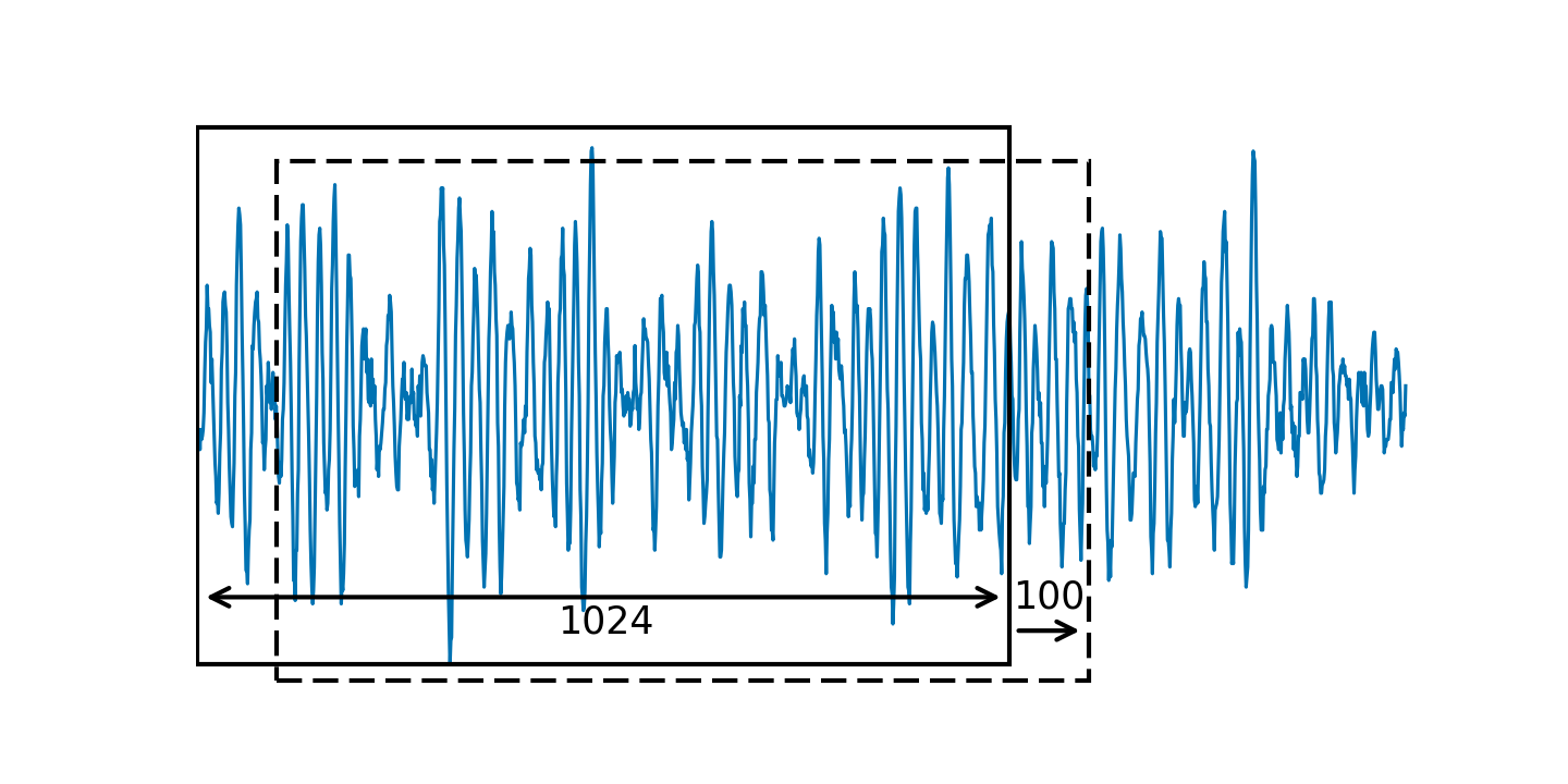
"We'll split the signal into slices of 1024 samples—that's about 0.02\n",
"seconds of audio. Why we choose 1024 and not 1000 we'll explain in a\n",
"second when we examine performance. The slices will overlap by 100\n",
"samples as shown here:\n",
"\n",
"\n",
"\n",
"Start by chopping up the signal into slices of 1024 samples, each\n",
"slice overlapping the previous by 100 samples. The resulting `slices`\n",
"object contains one slice per row."
]
},
{
"cell_type": "code",
"execution_count": null,
"metadata": {},
"outputs": [],
"source": [
"from skimage import util\n",
"\n",
"M = 1024\n",
"\n",
"slices = util.view_as_windows(audio, window_shape=(M,), step=100)\n",
"print(f'Audio shape: {audio.shape}, Sliced audio shape: {slices.shape}')"
]
},
{
"cell_type": "markdown",
"metadata": {},
"source": [
"Generate a windowing function (see the section on windowing for a\n",
"discussion of the underlying assumptions and interpretations of each)\n",
"and multiply it with the signal:"
]
},
{
"cell_type": "code",
"execution_count": null,
"metadata": {},
"outputs": [],
"source": [
"win = np.hanning(M + 1)[:-1]\n",
"slices = slices * win"
]
},
{
"cell_type": "markdown",
"metadata": {},
"source": [
"It's more convenient to have one slice per column, so we take the transpose:"
]
},
{
"cell_type": "code",
"execution_count": null,
"metadata": {},
"outputs": [],
"source": [
"slices = slices.T\n",
"print('Shape of `slices`:', slices.shape)"
]
},
{
"cell_type": "markdown",
"metadata": {},
"source": [
"For each slice, calculate the discrete Fourier transform. The DFT\n",
"returns both positive and negative frequencies (more on that in\n",
"\"Frequencies and their ordering\"), so we slice out the positive M / 2\n",
"frequencies for now."
]
},
{
"cell_type": "code",
"execution_count": null,
"metadata": {},
"outputs": [],
"source": [
"spectrum = np.fft.fft(slices, axis=0)[:M // 2 + 1:-1]\n",
"spectrum = np.abs(spectrum)"
]
},
{
"cell_type": "markdown",
"metadata": {},
"source": [
"(As a quick aside, you'll note that we use `scipy.fftpack.fft` and\n",
"`np.fft` interchangeably. NumPy provides basic FFT functionality,\n",
"which SciPy extends further, but both include an `fft` function, based\n",
"on the Fortran FFTPACK.)\n",
"\n",
"The spectrum can contain both very large and very small values.\n",
"Taking the log compresses the range significantly.\n",
"\n",
"Here we do a log plot of the ratio of the signal divided by the maximum signal.\n",
"The specific unit used for the ratio is the decibel, $20\n",
"log_{10}\\left(\\mathrm{amplitude ratio}\\right)$."
]
},
{
"cell_type": "code",
"execution_count": null,
"metadata": {},
"outputs": [],
"source": [
"f, ax = plt.subplots(figsize=(4.8, 2.4))\n",
"\n",
"S = np.abs(spectrum)\n",
"S = 20 * np.log10(S / np.max(S))\n",
"\n",
"ax.imshow(S, origin='lower', cmap='viridis',\n",
" extent=(0, L, 0, rate / 2 / 1000))\n",
"ax.axis('tight')\n",
"ax.set_ylabel('Frequency [kHz]')\n",
"ax.set_xlabel('Time [s]');"
]
},
{
"cell_type": "markdown",
"metadata": {},
"source": [
"\n",
"\n",
"Much better! We can now see the frequencies vary over time, and it\n",
"corresponds to the way the audio sounds. See if you can match my\n",
"earlier description: chee-chee-woorrrr-hee-hee cheet-wheet-hoorrr-chi\n",
"rrr-whi-wheo-wheo-wheo-wheo-wheo-wheo (I didn't transcribe the section\n",
"from 3 to 5 seconds—that's another bird).\n",
"\n",
"SciPy already includes an implementation of this\n",
"procedure as ``scipy.signal.spectrogram``, which can be invoked as\n",
"follows:"
]
},
{
"cell_type": "code",
"execution_count": null,
"metadata": {},
"outputs": [],
"source": [
"from scipy import signal\n",
"\n",
"freqs, times, Sx = signal.spectrogram(audio, fs=rate, window='hanning',\n",
" nperseg=1024, noverlap=M - 100,\n",
" detrend=False, scaling='spectrum')\n",
"\n",
"f, ax = plt.subplots(figsize=(4.8, 2.4))\n",
"ax.pcolormesh(times, freqs / 1000, 10 * np.log10(Sx), cmap='viridis')\n",
"ax.set_ylabel('Frequency [kHz]')\n",
"ax.set_xlabel('Time [s]');"
]
},
{
"cell_type": "markdown",
"metadata": {},
"source": [
"\n",
"\n",
"The only differences are that SciPy returns the spectrum magnitude\n",
"squared (which turns measured voltage into measured energy), and\n",
"multiplies it by some normalization factors[^scaling].\n",
"\n",
"[^scaling]: SciPy goes to some effort to preserve the energy in the\n",
" spectrum. Therefore, when taking only half the components\n",
" (for N even), it multiplies the remaining components,\n",
" apart from the first and last components, by two (those\n",
" two components are \"shared\" by the two halves of the\n",
" spectrum). It also normalizes the window by dividing it\n",
" by its sum.\n",
"\n",
"## History\n",
"\n",
"Tracing the exact origins of the Fourier transform is tricky. Some\n",
"related procedures go as far back as Babylonian times, but it was the\n",
"hot topics of calculating asteroid orbits and solving the heat (flow)\n",
"equation that led to several breakthroughs in the early 1800s. Whom\n",
"exactly among Clairaut, Lagrange, Euler, Gauss and D'Alembert we\n",
"should thank is not exactly clear, but Gauss was the first to describe\n",
"the fast Fourier transform (an algorithm for computing the discrete\n",
"Fourier transform, popularized by Cooley and Tukey in 1965). Joseph\n",
"Fourier, after whom the transform is named, first claimed that\n",
"*arbitrary* periodic [^periodic] functions can be expressed as a sum of\n",
"trigonometric functions.\n",
"\n",
"[^periodic]: The period can, in fact, also be infinite! The general\n",
" continuous Fourier transform provides for this\n",
" possibility. Discrete Fourier transforms are generally\n",
" defined over a finite interval, and this is implicitly\n",
" the period of the time domain function that is\n",
" transformed. In other words, if you do the inverse\n",
" discrete Fourier transform, you *always* get a periodic\n",
" signal out.\n",
"\n",
"## Implementation\n",
"\n",
"The discrete Fourier transform functionality in SciPy lives in the\n",
"`scipy.fftpack`` module. Among other things, it provides the\n",
"following DFT-related functionality:\n",
"\n",
" - ``fft``, ``fft2``, ``fftn``: Compute the discrete Fourier transform using\n",
" the Fast Fourier Transform algorithm in 1, 2, or `n` dimensions.\n",
" - ``ifft``, ``ifft2``, ``ifftn``: Compute the inverse of the DFT\n",
" - ``dct``, ``idct``, ``dst``, ``idst``: Compute the cosine and sine transforms, and their inverses.\n",
" - ``fftshift``, ``ifftshift``: Shift the zero-frequency component to the center of the spectrum and back, respectively (more about that soon).\n",
" - ``fftfreq``: Return the discrete Fourier transform sample frequencies.\n",
" - ``rfft``: Compute the DFT of a real sequence, exploiting the symmetry of the resulting spectrum for increased performance. Also used by ``fft`` internally when applicable.\n",
"\n",
"This is complemented by the following functions in NumPy:\n",
"\n",
" - ``np.hanning``, ``np.hamming``, ``np.bartlett``, ``np.blackman``,\n",
" ``np.kaiser``: Tapered windowing functions.\n",
"\n",
"It is also used to perform fast convolutions of large inputs by\n",
"``scipy.signal.fftconvolve`.\n",
"\n",
"SciPy wraps the Fortran FFTPACK library—it is not the fastest out\n",
"there, but unlike packages such as FFTW, it has a permissive free\n",
"software license.\n",
"\n",
"## Choosing the length of the discrete Fourier transform (DFT)\n",
"\n",
"A naive calculation of the DFT takes $\\mathcal{O}\\left(N^2\\right)$ operations [^big_O].\n",
"How come? Well, you have $N$\n",
"(complex) sinusoids of different frequencies ($2 \\pi f \\times 0, 2 \\pi f \\times\n",
"1, 2 \\pi f \\times 3, ..., 2 \\pi f \\times (N - 1)$), and you want to see how\n",
"strongly your signal corresponds to each. Starting with the first,\n",
"you take the dot product with the signal (which, in itself, entails $N$\n",
"multiplication operations). Repeating this operation$N$times, once\n",
"for each sinusoid, then gives $N^2$ operations.\n",
"\n",
"[^big_O]: In computer science, the computational cost of an algorithm\n",
" is often expressed in \"Big O\" notation. The notation gives\n",
" us an indication of how an algorithm's execution time scales\n",
" with an increasing number of elements. If an algorithm is $\\mathcal{O}(N)$,\n",
" it means its execution time increases linearly with\n",
" the number of input elements (for example, searching for a\n",
" given value in an unsorted list is $\\mathcal{O}\\left(N\\right)$). Bubble sort is\n",
" an example of an $O\\left(N^2\\right)$ algorithm; the exact number of\n",
" operations performed may, hypothetically, be $N + \\frac{1}{2} N^2$,\n",
" meaning that the computational cost grows quadratically with\n",
" the number of input elements.\n",
"\n",
"Now, contrast that with the fast Fourier transform, which is $\\mathcal{O}\\left(N \\log N\\right)$ in\n",
"the ideal case due to the clever re-use of\n",
"calculations—a great improvement! However, the classical Cooley-Tukey\n",
"algorithm implemented in FFTPACK (and used by SciPy) recursively breaks up the transform\n",
"into smaller (prime-sized) pieces and only shows this improvement for\n",
"\"smooth\" input lengths (an input length is considered smooth when its\n",
"largest prime factor is small). For large prime sized pieces, the\n",
"Bluestein or Rader algorithms can be used in conjunction with the\n",
"Cooley-Tukey algorithm, but this optimization is not implemented in\n",
"FFTPACK.[^fast]\n",
"\n",
"Let us illustrate:"
]
},
{
"cell_type": "code",
"execution_count": null,
"metadata": {},
"outputs": [],
"source": [
"import time\n",
"\n",
"from scipy import fftpack\n",
"from sympy import factorint\n",
"\n",
"K = 1000\n",
"lengths = range(250, 260)\n",
"\n",
"# Calculate the smoothness for all input lengths\n",
"smoothness = [max(factorint(i).keys()) for i in lengths]\n",
"\n",
"\n",
"exec_times = []\n",
"for i in lengths:\n",
" z = np.random.random(i)\n",
"\n",
" # For each input length i, execute the FFT K times\n",
" # and store the execution time\n",
"\n",
" times = []\n",
" for k in range(K):\n",
" tic = time.monotonic()\n",
" fftpack.fft(z)\n",
" toc = time.monotonic()\n",
" times.append(toc - tic)\n",
"\n",
" # For each input length, remember the *minimum* execution time\n",
" exec_times.append(min(times))\n",
"\n",
"\n",
"f, (ax0, ax1) = plt.subplots(2, 1, sharex=True)\n",
"ax0.stem(lengths, np.array(exec_times) * 10**6)\n",
"ax0.set_ylabel('Execution time (µs)')\n",
"\n",
"ax1.stem(lengths, smoothness)\n",
"ax1.set_ylabel('Smoothness of input length\\n(lower is better)')\n",
"ax1.set_xlabel('Length of input');"
]
},
{
"cell_type": "markdown",
"metadata": {},
"source": [
"\n",
"\n",
"The intuition is that, for smooth numbers, the FFT can be broken up\n",
"into many small pieces. After performing the FFT on the first piece,\n",
"those results can be reused in subsequent computations. This explains\n",
"why we chose a length of 1024 for our audio slices earlier—it has a\n",
"smoothness of only 2, resulting in the optimal \"radix-2 Cooley-Tukey\"\n",
"algorithm, which computes the FFT using only $(N/2) \\log_2 N = 5120$ complex\n",
"multiplications, instead of $N^2 = 1048576$. Choosing $N = 2^m$\n",
"always ensures a maximally smooth $N$ (and, thus, the fastest FFT).\n",
"\n",
"[^fast]: While ideally we don't want to reimplement existing\n",
" algorithms, sometimes it becomes necessary in order to obtain\n",
" the best execution speeds possible, and tools\n",
" like [Cython](http://cython.org)—which compiles Python to\n",
" C—and [Numba](http://numba.pydata.org)—which does\n",
" just-in-time compilation of Python code—make life a lot\n",
" easier (and faster!). If you are able to use GPL-licenced\n",
" software, you may consider\n",
" using [PyFFTW](https://github.com/hgomersall/pyFFTW) for\n",
" faster FFTs.\n",
"\n",
"## More discrete Fourier transform concepts\n",
"\n",
"Next, we present a couple of common concepts worth knowing before\n",
"operating heavy Fourier transform machinery, whereafter we tackle\n",
"another real-world problem: analyzing target detection in radar data.\n",
"\n",
"### Frequencies and their ordering\n",
"\n",
"For historical reasons, most implementations return an array where\n",
"frequencies vary from low-to-high-to-low (see the box \"Discrete\n",
"Fourier transforms\" for further explanation of frequencies). E.g., when we do the real\n",
"Fourier transform of a signal of all ones, an input that has no\n",
"variation and therefore only has the slowest, constant Fourier\n",
"component (also known as the \"DC\" or Direct Current component—just\n",
"electronics jargon for \"mean of the signal\"), appearing as the first\n",
"entry:"
]
},
{
"cell_type": "code",
"execution_count": null,
"metadata": {},
"outputs": [],
"source": [
"from scipy import fftpack\n",
"N = 10\n",
"\n",
"fftpack.fft(np.ones(N)) # The first component is np.mean(x) * N"
]
},
{
"cell_type": "markdown",
"metadata": {},
"source": [
"When we try the FFT on a rapidly changing signal, we see a high\n",
"frequency component appear:"
]
},
{
"cell_type": "code",
"execution_count": null,
"metadata": {},
"outputs": [],
"source": [
"z = np.ones(10)\n",
"z[::2] = -1\n",
"\n",
"print(f'Applying FFT to {z}')\n",
"fftpack.fft(z)"
]
},
{
"cell_type": "markdown",
"metadata": {},
"source": [
"Note that the FFT returns a complex spectrum which, in the case of\n",
"real inputs, is conjugate symmetrical (i.e., symmetric in the real\n",
"part, and anti-symmetric in the imaginary part):"
]
},
{
"cell_type": "code",
"execution_count": null,
"metadata": {},
"outputs": [],
"source": [
"x = np.array([1, 5, 12, 7, 3, 0, 4, 3, 2, 8])\n",
"X = fftpack.fft(x)\n",
"\n",
"with np.printoptions(precision=2):\n",
" print(\"Real part: \", X.real)\n",
" print(\"Imaginary part:\", X.imag)"
]
},
{
"cell_type": "markdown",
"metadata": {},
"source": [
"(And, again, recall that the first component is ``np.mean(x) * N``.)\n",
"\n",
"The `fftfreq` function tells us which frequencies we are looking at\n",
"specifically:"
]
},
{
"cell_type": "code",
"execution_count": null,
"metadata": {},
"outputs": [],
"source": [
"fftpack.fftfreq(10)"
]
},
{
"cell_type": "markdown",
"metadata": {},
"source": [
"The result tells us that our maximum component occured at a frequency\n",
"of 0.5 cycles per sample. This agrees with the input, where a\n",
"minus-one-plus-one cycle repeated every second sample.\n",
"\n",
"Sometimes, it is convenient to view the spectrum organized slightly\n",
"differently, from high-negative to low to-high-positive (for now, we\n",
"won't dive too deeply into the concept of negative frequency, other\n",
"than saying a real-world sine wave is produced by a combination of\n",
"positive and negative frequencies). We re-shuffle the spectrum using\n",
"the `fftshift` function.\n",
"\n",
"> **Discrete Fourier transforms {.callout}**\n",
">\n",
"> The Discrete Fourier Transform (DFT) converts a sequence of $N$\n",
"> equally spaced real or complex samples $x_{0,}x_{1,\\ldots x_{N-1}}$ of\n",
"> a function $x(t)$ of time (or another variable, depending on the\n",
"> application) into a sequence of $N$ complex numbers $X_{k}$ by the\n",
"> summation\n",
">\n",
"> $$X_{k}=\\sum_{n=0}^{N-1}x_{n}e^{-j2\\pi kn/N},\\;k=0,1,\\ldots\n",
"> N-1.$$\n",
">\n",
"> With the numbers $X_{k}$ known, the inverse DFT *exactly* recovers the\n",
"> sample values $x_{n}$ through the summation\n",
">\n",
"> $$x_{n}=\\frac{1}{N}\\sum_{k=0}^{N-1}X_{k}e^{j2\\pi kn/N}.$$\n",
">\n",
"> Keeping in mind that $e^{j\\theta}=\\cos\\theta+j\\sin\\theta,$ the last\n",
"> equation shows that the DFT has decomposed the sequence $x_{n}$ into a\n",
"> complex discrete Fourier series with coefficients $X_{k}$. Comparing\n",
"> the DFT with a continuous complex Fourier series\n",
">\n",
"> $$x(t)=\\sum_{n=-\\infty}^{\\infty}c_{n}e^{jn\\omega_{0}t},$$\n",
">\n",
"> the DFT is a *finite *series with $N$ terms defined at the equally\n",
"> spaced discrete instances of the *angle* $(\\omega_{0}t_{n})=2\\pi\\frac{k}{N}$\n",
"> in the interval $[0,2\\pi)$,\n",
"> i.e. *including* $0$ and *excluding* $2\\pi$.\n",
"> This automatically normalizes the DFT so that time does\n",
"> not appear explicitly in the forward or inverse transform.\n",
">\n",
"> If the original function $x(t)$ is limited in frequency to less than\n",
"> half of the sampling frequency (the so-called *Nyquist frequency*),\n",
"> interpolation between sample values produced by the inverse DFT will\n",
"> usually give a faithful reconstruction of $x(t)$. If $x(t)$ is *not*\n",
"> limited as such, the inverse DFT can, in general, not be used to\n",
"> reconstruct $x(t)$ by interpolation. Note that this limit does not\n",
"> imply that there are *no* methods that can do such a\n",
"> reconstruction—see, e.g., compressed sensing, or finite rate of\n",
"> innovation sampling.\n",
">\n",
"> The function $e^{j2\\pi k/N}=\\left(e^{j2\\pi/N}\\right)^{k}=w^{k}$ takes on\n",
"> discrete values between $0$ and $2\\pi\\frac{N-1}{N}$ on the unit circle in\n",
"> the complex plane. The function $e^{j2\\pi kn/N}=w^{kn}$ encircles the\n",
"> origin $n\\frac{N-1}{N}$ times, thus generating harmonics of the fundamental\n",
"> sinusoid for which $n=1$.\n",
">\n",
"> The way in which we defined the DFT leads to a few subtleties\n",
"> when $n>\\frac{N}{2}$, for even $N$ [^odd_N]. The function $e^{j2\\pi kn/N}$ is plotted\n",
"> for increasing values of $k$ in the figure below,\n",
"> for the cases $n=1$ to $n=N-1$ for $N=16$. When $k$ increases from $k$\n",
"> to $k+1$, the angle increases by $\\frac{2\\pi n}{N}$. When $n=1$,\n",
"> the step is $\\frac{2\\pi}{N}$. When $n=N-1$, the angle\n",
"> increases by $2\\pi\\frac{N-1}{N}=2\\pi-\\frac{2\\pi}{N}$. Since $2\\pi$\n",
"> is precisely once around the circle, the step equates to $-\\frac{2\\pi}{N}$,\n",
"> i.e. in the direction of a negative\n",
"> frequency. The components up to $N/2$ represent *positive* frequency\n",
"> components, those above $N/2$ up to $N-1$ represent *negative*\n",
"> frequencies. The angle increment for the component $N/2$\n",
"> for $N$ even advances precisely halfway around the circle for\n",
"> each increment in $k$ and can therefore be interpreted as either a\n",
"> positive or a negative frequency. This component of the DFT represents\n",
"> the Nyquist Frequency, i.e. half of the sampling frequency, and is\n",
"> useful to orientate oneself when looking at DFT graphics.\n",
">\n",
"> The FFT in turn is simply a special and highly efficient algorithm for\n",
"> calculating the DFT. Whereas a straightforward calculation of the DFT\n",
"> takes of the order of $N^{2}$ calculations to compute, the FFT\n",
"> algorithm requires of the order $N\\log N$ calculations. The FFT was\n",
"> the key to the wide-spread use of the DFT in real-time applications\n",
"> and was included in a list of the top $10$ algorithms of the $20^{th}$\n",
"> century by the IEEE journal Computing in Science & Engineering in the\n",
"> year $2000$.\n",
">\n",
"> \n",
"\n",
"[^odd_N]: We leave it as an exercise for the reader to picture the\n",
" situation for $N$ odd. In this chapter, all examples use\n",
" even-order DFTs.\n",
"\n",
"Let's examine the frequency components in a noisy image. Note that,\n",
"while a static image has no time-varying component, its values do vary\n",
"across *space*. The DFT applies equally to either case.\n",
"\n",
"First, load and display the image:"
]
},
{
"cell_type": "code",
"execution_count": null,
"metadata": {},
"outputs": [],
"source": [
"from skimage import io\n",
"image = io.imread('images/moonlanding.png')\n",
"M, N = image.shape\n",
"\n",
"f, ax = plt.subplots(figsize=(4.8, 4.8))\n",
"ax.imshow(image)\n",
"\n",
"print((M, N), image.dtype)"
]
},
{
"cell_type": "markdown",
"metadata": {},
"source": [
"\n",
"\n",
"Do not adjust your monitor! The image you are seeing is real,\n",
"although clearly distorted by either the measurement or transmission\n",
"equipment.\n",
"\n",
"To examine the spectrum of the image, we use `fftn` (instead of `fft`)\n",
"to compute the DFT, since it has more than one dimension. The\n",
"two-dimensional FFT is equivalent to taking the 1-D FFT across rows\n",
"and then across columns (or vice versa)."
]
},
{
"cell_type": "code",
"execution_count": null,
"metadata": {},
"outputs": [],
"source": [
"F = fftpack.fftn(image)\n",
"\n",
"F_magnitude = np.abs(F)\n",
"F_magnitude = fftpack.fftshift(F_magnitude)\n"
]
},
{
"cell_type": "markdown",
"metadata": {},
"source": [
"Again, we take the log of the spectrum to compress the range of\n",
"values, before displaying:"
]
},
{
"cell_type": "code",
"execution_count": null,
"metadata": {},
"outputs": [],
"source": [
"f, ax = plt.subplots(figsize=(4.8, 4.8))\n",
"\n",
"ax.imshow(np.log(1 + F_magnitude), cmap='viridis',\n",
" extent=(-N // 2, N // 2, -M // 2, M // 2))\n",
"ax.set_title('Spectrum magnitude');"
]
},
{
"cell_type": "markdown",
"metadata": {},
"source": [
"\n",
"\n",
"Note the high values around the origin (middle) of the spectrum—these\n",
"coefficients describe the low frequencies or smooth parts of the\n",
"image; a vague canvas of the photo. Higher frequency components,\n",
"spread throughout the spectrum, fill in the edges and detail. Peaks\n",
"around higher frequencies correspond to the periodic noise.\n",
"\n",
"From the photo, we can see that the noise (measurement artifacts) is\n",
"highly periodic, so we hope to remove it by zeroing out the\n",
"corresponding parts of the spectrum.\n",
"\n",
"The image with those peaks suppressed indeed looks quite different!"
]
},
{
"cell_type": "code",
"execution_count": null,
"metadata": {},
"outputs": [],
"source": [
"# Set block around center of spectrum to zero\n",
"K = 40\n",
"F_magnitude[M // 2 - K: M // 2 + K, N // 2 - K: N // 2 + K] = 0\n",
"\n",
"# Find all peaks higher than the 98th percentile\n",
"peaks = F_magnitude < np.percentile(F_magnitude, 98)\n",
"\n",
"# Shift the peaks back to align with the original spectrum\n",
"peaks = fftpack.ifftshift(peaks)\n",
"\n",
"# Make a copy of the original (complex) spectrum\n",
"F_dim = F.copy()\n",
"\n",
"# Set those peak coefficients to zero\n",
"F_dim = F_dim * peaks.astype(int)\n",
"\n",
"# Do the inverse Fourier transform to get back to an image\n",
"# Since we started with a real image, we only look at the real part of\n",
"# the output.\n",
"image_filtered = np.real(fftpack.ifft2(F_dim))\n",
"\n",
"f, (ax0, ax1) = plt.subplots(2, 1, figsize=(4.8, 7))\n",
"ax0.imshow(fftpack.fftshift(np.log10(1 + np.abs(F_dim))), cmap='viridis')\n",
"ax0.set_title('Spectrum after suppression')\n",
"\n",
"ax1.imshow(image_filtered)\n",
"ax1.set_title('Reconstructed image');"
]
},
{
"cell_type": "markdown",
"metadata": {},
"source": [
"\n",
"\n",
"### Windowing\n",
"\n",
"If we examine the Fourier transform of a rectangular pulse, we see\n",
"significant sidelobes in the spectrum:"
]
},
{
"cell_type": "code",
"execution_count": null,
"metadata": {},
"outputs": [],
"source": [
"x = np.zeros(500)\n",
"x[100:150] = 1\n",
"\n",
"X = fftpack.fft(x)\n",
"\n",
"f, (ax0, ax1) = plt.subplots(2, 1, sharex=True)\n",
"\n",
"ax0.plot(x)\n",
"ax0.set_ylim(-0.1, 1.1)\n",
"\n",
"ax1.plot(fftpack.fftshift(np.abs(X)))\n",
"ax1.set_ylim(-5, 55);"
]
},
{
"cell_type": "markdown",
"metadata": {},
"source": [
"\n",
"\n",
"In theory, you would need a combination of infinitely many sinusoids\n",
"(frequencies) to represent any abrupt transition; the coefficients would\n",
"typically have the same sidelobe structure as seen here for the pulse.\n",
"\n",
"Importantly, the discrete Fourier transform assumes that the input\n",
"signal is periodic. If the signal is not, the assumption is simply\n",
"that, right at the end of the signal, it jumps back to its beginning\n",
"value. Consider the function, $x(t)$, shown here:\n",
"\n",
" \n",
"\n",
"\n",
"We only measure the signal for a short time, labeled $T_{eff}$. The\n",
"Fourier transform assumes that $x(8) = x(0)$, and that the signal is\n",
"continued as the dashed, rather than the solid line. This introduces\n",
"a big jump at the edge, with the expected oscillation in the spectrum:"
]
},
{
"cell_type": "code",
"execution_count": null,
"metadata": {},
"outputs": [],
"source": [
"t = np.linspace(0, 1, 500)\n",
"x = np.sin(49 * np.pi * t)\n",
"\n",
"X = fftpack.fft(x)\n",
"\n",
"f, (ax0, ax1) = plt.subplots(2, 1)\n",
"\n",
"ax0.plot(x)\n",
"ax0.set_ylim(-1.1, 1.1)\n",
"\n",
"ax1.plot(fftpack.fftfreq(len(t)), np.abs(X))\n",
"ax1.set_ylim(0, 190);"
]
},
{
"cell_type": "markdown",
"metadata": {},
"source": [
"\n",
"\n",
"Instead of the expected two lines, the peaks are spread out in the\n",
"spectrum.\n",
"\n",
"We can counter this effect by a process called *windowing*. The\n",
"original function is multiplied with a window function such as the\n",
"Kaiser window $K(N,\\beta)$. Here we visualize it for $\\beta$ ranging\n",
"from 0 to 100:"
]
},
{
"cell_type": "code",
"execution_count": null,
"metadata": {},
"outputs": [],
"source": [
"f, ax = plt.subplots()\n",
"\n",
"N = 10\n",
"beta_max = 5\n",
"colormap = plt.cm.plasma\n",
"\n",
"norm = plt.Normalize(vmin=0, vmax=beta_max)\n",
"\n",
"lines = [\n",
" ax.plot(np.kaiser(100, beta), color=colormap(norm(beta)))\n",
" for beta in np.linspace(0, beta_max, N)\n",
" ]\n",
"\n",
"sm = plt.cm.ScalarMappable(cmap=colormap, norm=norm)\n",
"\n",
"sm._A = []\n",
"\n",
"plt.colorbar(sm).set_label(r'Kaiser $\\beta$');"
]
},
{
"cell_type": "markdown",
"metadata": {},
"source": [
"\n",
"\n",
"By changing the parameter $\\beta$, the shape of the window can be\n",
"changed from rectangular ($\\beta=0$, no windowing) to a window that\n",
"produces signals that smoothly increase from zero and decrease to zero\n",
"at the endpoints of the sampled interval, producing very low side\n",
"lobes ($\\beta$ typically between 5 and 10) [^choosing_a_window].\n",
"\n",
"[^choosing_a_window]: The classical windowing functions include Hann,\n",
" Hamming, and Blackman. They differ in their\n",
" sidelobe levels and in the broadening of the\n",
" main lobe (in the Fourier domain). A modern and\n",
" flexible window function that is close to\n",
" optimal for most applications is the Kaiser\n",
" window—a good approximation to the optimal\n",
" prolate spheroid window, which concentrates the\n",
" most energy into the main lobe. The Kaiser\n",
" window can be tuned to suit the particular\n",
" application, as illustrated in the main text, by\n",
" adjusting the parameter $\\beta$.\n",
"\n",
"Applying the Kaiser window here, we see that the sidelobes have been\n",
"drastically reduced, at the cost of a slight widening in the main lobe.\n",
"\n",
"\n",
"\n",
"The effect of windowing our previous example is noticeable:"
]
},
{
"cell_type": "code",
"execution_count": null,
"metadata": {},
"outputs": [],
"source": [
"win = np.kaiser(len(t), 5)\n",
"X_win = fftpack.fft(x * win)\n",
"\n",
"plt.plot(fftpack.fftfreq(len(t)), np.abs(X_win))\n",
"plt.ylim(0, 190);"
]
},
{
"cell_type": "markdown",
"metadata": {},
"source": [
"\n",
"\n",
"## Real-world Application: Analyzing Radar Data\n",
"\n",
"Linearly modulated FMCW (Frequency-Modulated Continuous-Wave) radars\n",
"make extensive use of the FFT algorithm for signal processing and\n",
"provide examples of various applications of the FFT. We will use actual\n",
"data from an FMCW radar to demonstrate one such an application: target\n",
"detection.\n",
"\n",
"Roughly, an FMCW radar works like this (see box \"A\n",
"simple FMCW radar system\" for more detail):\n",
"\n",
"A signal with changing frequency is generated. This signal is\n",
"transmitted by an antenna, after which it travels outwards, away from the\n",
"radar. When it hits an object, part of the signal is reflected back\n",
"to the radar, where it is received, multiplied by a copy of the\n",
"transmitted signal, and sampled, turning it into\n",
"numbers that are packed into an array. Our challenge is to interpret\n",
"those numbers to form meaningful results.\n",
"\n",
"The multiplication step above is important. From school, recall the\n",
"trigonometric identity:\n",
"\n",
"$\n",
"\\sin(xt) \\sin(yt) = \\frac{1}{2}\n",
"\\left[ \\sin \\left( (x - y)t + \\frac{\\pi}{2} \\right) - \\sin \\left( (x + y)t + \\frac{\\pi}{2} \\right) \\right]\n",
"$\n",
"\n",
"Thus, if we multiply the received signal by the transmitted signal, we\n",
"expect two frequency components to appear in the spectrum: one that is\n",
"the difference in frequencies between the received and transmitted\n",
"signal, and one that is the sum of their frequencies.\n",
"\n",
"We are particularly interested in the first, since that gives us some\n",
"indication of how long it took the signal to reflect back to the radar\n",
"(in other words, how far away the object is from us!). We discard the\n",
"other by applying a low-pass filter to the signal (i.e., a filter that\n",
"discards any high frequencies).\n",
"\n",
"> **A simple FMCW radar system** {.callout}\n",
">\n",
"> \n",
">\n",
"> A block diagram of a simple FMCW radar that uses separate\n",
"> transmit and receive antennas is shown above. The radar consists of a waveform generator\n",
"> that generates a sinusoidal signal of which the frequency varies\n",
"> linearly around the required transmit frequency. The generated signal\n",
"> is amplified to the required power level by the transmit amplifier\n",
"> and routed to the transmit antenna via a coupler circuit where a copy\n",
"> of the transmit signal is tapped off. The transmit antenna radiates\n",
"> the transmit signal as an electromagnetic wave in a narrow beam\n",
"> towards the target to be detected. When the wave encounters an object\n",
"> that reflects electromagnetic waves, a fraction of of the energy\n",
"> irradiating the target is reflected back to the receiver as a second\n",
"> electromagnetic wave that propagates in the direction of the radar\n",
"> system. When this wave encounters the receive antenna, the antenna\n",
"> collects the energy in the wave energy impinging on it and converts\n",
"> it to a fluctuating voltage that is fed to the mixer. The mixer\n",
"> multiplies the received signal with a replica of the transmit signal\n",
"> and produces a sinusoidal signal with a frequency equal to the\n",
"> difference in frequency between the transmitted and received\n",
"> signals. The low-pass filter ensures that the received signal is band\n",
"> limited (i.e., does not contain frequencies that we don't care about)\n",
"> and the receive amplifier strengthens the signal to a suitable\n",
"> amplitude for the analog to digital converter (ADC) that feeds data\n",
"> to the computer.\n",
"\n",
"To summarize, we should note that:\n",
"\n",
" - The data that reaches the computer consists of $N$ samples sampled\n",
" (from the multiplied, filtered signal) at a sample frequency of\n",
" $f_{s}$.\n",
" - The **amplitude** of the returned signal varies depending on the\n",
" **strength of the reflection** (i.e., is a property of the target\n",
" object and the distance between the target and the radar).\n",
" - The **frequency measured** is an indication of the **distance** of the\n",
" target object from the radar.\n",
"\n",
"\n",
"\n",
"\n",
"\n",
"To start off, we'll generate some synthetic signals, after which we'll\n",
"turn our focus to the output of an actual radar.\n",
"\n",
"Recall that the radar is increasing its frequency as it transmits at a\n",
"rate of $S$ Hz/s. After a certain amount of time, $t$, has passed,\n",
"the frequency will now be $t S$ higher. In that same time span, the\n",
"radar signal has traveled $d = t / v$ meters, where $v$ is the speed of\n",
"the transmitted wave through air (roughly the same as the speed of\n",
"light, $3 \\times 10^8$ m/s).\n",
"\n",
"Combining the above observations, we can calculate the amount of time\n",
"it would take the signal to travel to, bounce off, and return from a\n",
"target that is distance $R$ away:\n",
"\n",
"$$ t_R = 2R / v $$\n",
"\n",
"Therefore, the change in frequency for a target at range $R$ will be:\n",
"\n",
"$$ f_{d}= t_R S = \\frac{2RS}{v}$$"
]
},
{
"cell_type": "code",
"execution_count": null,
"metadata": {},
"outputs": [],
"source": [
"pi = np.pi\n",
"\n",
"# Radar parameters\n",
"fs = 78125 # Sampling frequency in Hz, i.e. we sample 78125\n",
" # times per second\n",
"\n",
"ts = 1 / fs # Sampling time, i.e. one sample is taken each\n",
" # ts seconds\n",
"\n",
"Teff = 2048.0 * ts # Total sampling time for 2048 samples\n",
" # (AKA effective sweep duration) in seconds.\n",
"\n",
"Beff = 100e6 # Range of transmit signal frequency during the time the\n",
" # radar samples, known as the \"effective bandwidth\"\n",
" # (given in Hz)\n",
"\n",
"S = Beff / Teff # Frequency sweep rate in Hz/s\n",
"\n",
"# Specification of targets. We made these targets up, imagining they\n",
"# are objects seen by the radar with the specified range and size\n",
"\n",
"R = np.array([100, 137, 154, 159, 180]) # Ranges (in meter)\n",
"M = np.array([0.33, 0.2, 0.9, 0.02, 0.1]) # Target size\n",
"P = np.array([0, pi / 2, pi / 3, pi / 5, pi / 6]) # Randomly chosen phase offsets\n",
"\n",
"t = np.arange(2048) * ts # Sample times\n",
"\n",
"fd = 2 * S * R / 3E8 # Frequency differences for these targets\n",
"\n",
"# Generate five targets\n",
"signals = np.cos(2 * pi * fd * t[:, np.newaxis] + P)\n",
"\n",
"# Save the signal associated with the first target as an example for\n",
"# later inspection\n",
"v_single = signals[:, 0]\n",
"\n",
"# Weigh the signals, according to target size, and sum, to generate\n",
"# the combined signal seen by the radar\n",
"v_sim = np.sum(M * signals, axis=1)\n",
"\n",
"## The above code is equivalent to:\n",
"#\n",
"# v0 = np.cos(2 * pi * fd[0] * t)\n",
"# v1 = np.cos(2 * pi * fd[1] * t + pi / 2)\n",
"# v2 = np.cos(2 * pi * fd[2] * t + pi / 3)\n",
"# v3 = np.cos(2 * pi * fd[3] * t + pi / 5)\n",
"# v4 = np.cos(2 * pi * fd[4] * t + pi / 6)\n",
"#\n",
"## Blend them together\n",
"# v_single = v0\n",
"# v_sim = (0.33 * v0) + (0.2 * v1) + (0.9 * v2) + (0.02 * v3) + (0.1 * v4)\n"
]
},
{
"cell_type": "markdown",
"metadata": {},
"source": [
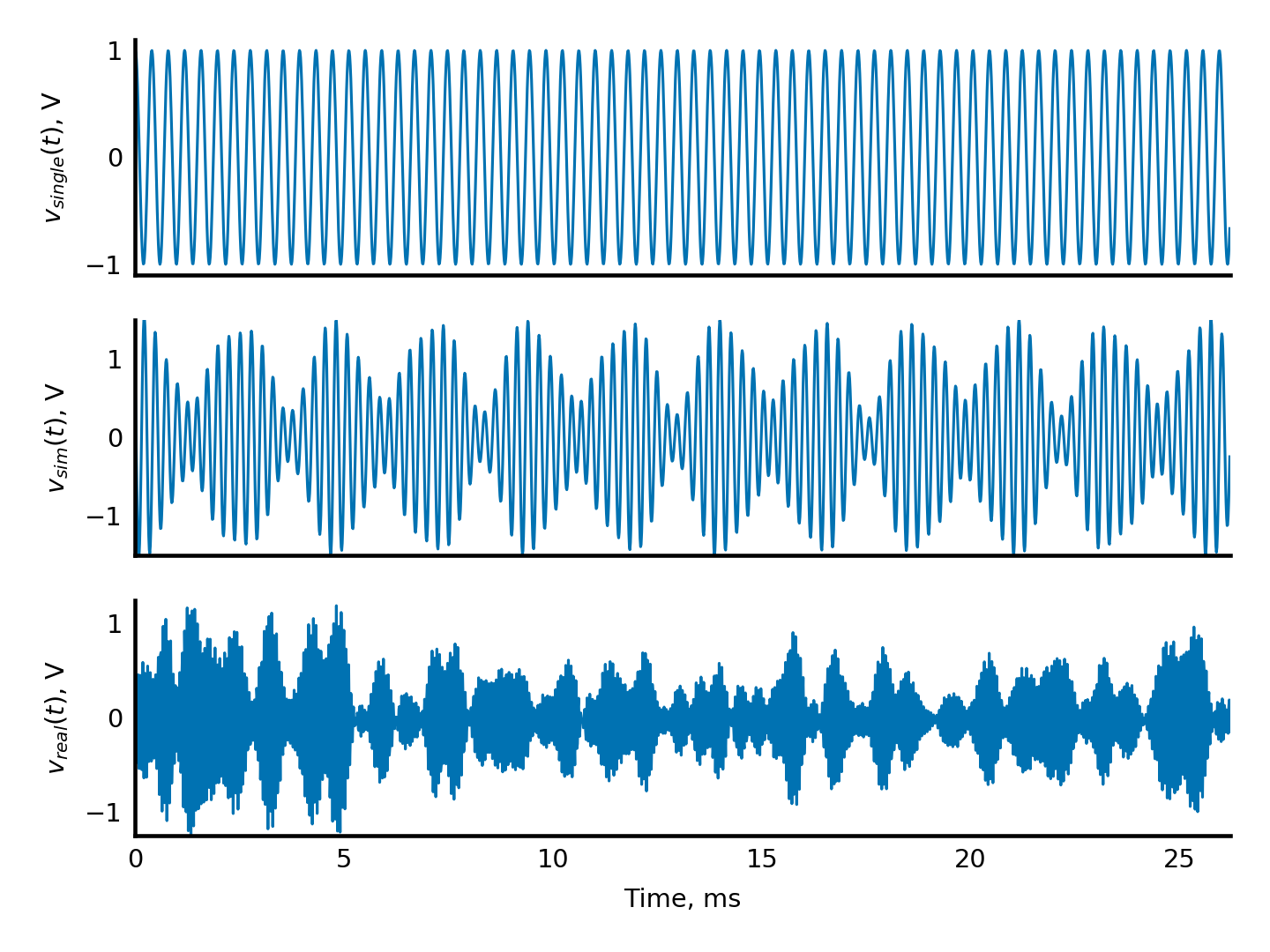
"Above, we generate a synthetic signal, $v_{single}$, received when\n",
"looking at a single target (see figure below). By counting the number\n",
"of cycles seen in a given time period, we can compute the frequency of\n",
"the signal and thus the distance to the target.\n",
"\n",
"A real radar will rarely receive only a single echo, though. The\n",
"simulated signal $v_\\mathrm{sim}$ shows what a radar signal will look\n",
"like with five targets at different ranges (including two close to one\n",
"another at 154 and 159 meters), and $v_\\mathrm{actual}(t)$ shows the\n",
"output signal obtained with an actual radar. When multiple echoes add\n",
"together, the result makes little intuitive sense; until, that is, we\n",
"look at it more carefully through the lens of the discrete Fourier\n",
"transform.\n",
"\n",
"\n",
"\n",
"\n",
"\n",
"The real world radar data is read from a NumPy-format ``.npz`` file (a\n",
"light-weight, cross platform and cross-version compatible storage\n",
"format). These files can be saved with the ``np.savez`` or\n",
"``np.savez_compressed`` functions. Note that SciPy's ``io`` submodule\n",
"can also easily read other formats, such as MATLAB(R) and NetCDF\n",
"files."
]
},
{
"cell_type": "code",
"execution_count": null,
"metadata": {},
"outputs": [],
"source": [
"data = np.load('data/radar_scan_0.npz')\n",
"\n",
"# Load variable 'scan' from 'radar_scan_0.npz'\n",
"scan = data['scan']\n",
"\n",
"# The dataset contains multiple measurements, each taken with the\n",
"# radar pointing in a different direction. Here we take one such as\n",
"# measurement, at a specified azimuth (left-right position) and elevation\n",
"# (up-down position). The measurement has shape (2048,).\n",
"\n",
"v_actual = scan['samples'][5, 14, :]\n",
"\n",
"# The signal amplitude ranges from -2.5V to +2.5V. The 14-bit\n",
"# analogue-to-digital converter in the radar gives out integers\n",
"# between -8192 to 8192. We convert back to voltage by multiplying by\n",
"# $(2.5 / 8192)$.\n",
"\n",
"v_actual = v_actual * (2.5 / 8192)\n"
]
},
{
"cell_type": "markdown",
"metadata": {},
"source": [
"Since ``.npz``-files can store multiple variables, we have to select\n",
"the one we want: ``data['scan']``. That returns a\n",
"*structured NumPy array* with the following fields:\n",
"\n",
"- **time** : unsigned 64-bit (8 byte) integer (`np.uint64`)\n",
"- **size** : unsigned 32-bit (4 byte) integer (`np.uint32`)\n",
"- **position**\n",
"\n",
" - **az** : 32-bit float (`np.float32`)\n",
" - **el** : 32-bit float (`np.float32`)\n",
" - **region_type** : unsigned 8-bit (1 byte) integer (`np.uint8`)\n",
" - **region_ID** : unsigned 16-bit (2 byte) integer (`np.uint16`)\n",
" - **gain** : unsigned 8-bit (1 byte) integer (`np.uin8`)\n",
" - **samples** : 2048 unsigned 16-bit (2 byte) integers (`np.uint16`)\n",
"\n",
"While it is true that NumPy arrays are *homogeneous* (i.e., all the\n",
"elements inside are the same), it does not mean that those elements\n",
"cannot be compound elements, as is the case here.\n",
"\n",
"An individual field is accessed using dictionary syntax:"
]
},
{
"cell_type": "code",
"execution_count": null,
"metadata": {},
"outputs": [],
"source": [
"azimuths = scan['position']['az'] # Get all azimuth measurements"
]
},
{
"cell_type": "markdown",
"metadata": {},
"source": [
"To summarize what we've seen so far: the shown measurements\n",
"($v_\\mathrm{sim}$ and $v_\\mathrm{actual}$) are the sum of sinusoidal\n",
"signals reflected by each of several objects. We need to determine\n",
"each of the constituent components of these composite radar\n",
"signals. The FFT is the tool that will do this for us.\n",
"\n",
"### Signal properties in the frequency domain\n",
"\n",
"First, we take the FFTs of our three signals (synthetic single target,\n",
"synthetic multi-target, and real) and then display the\n",
"positive frequency components (i.e., components $0$ to $N/2$). These\n",
"are called the *range traces* in radar terminology."
]
},
{
"cell_type": "code",
"execution_count": null,
"metadata": {},
"outputs": [],
"source": [
"fig, axes = plt.subplots(3, 1, sharex=True, figsize=(4.8, 2.4))\n",
"\n",
"# Take FFTs of our signals. Note the convention to name FFTs with a\n",
"# capital letter.\n",
"\n",
"V_single = np.fft.fft(v_single)\n",
"V_sim = np.fft.fft(v_sim)\n",
"V_actual = np.fft.fft(v_actual)\n",
"\n",
"N = len(V_single)\n",
"\n",
"with plt.style.context('style/thinner.mplstyle'):\n",
" axes[0].plot(np.abs(V_single[:N // 2]))\n",
" axes[0].set_ylabel(\"$|V_\\mathrm{single}|$\")\n",
" axes[0].set_xlim(0, N // 2)\n",
" axes[0].set_ylim(0, 1100)\n",
"\n",
" axes[1].plot(np.abs(V_sim[:N // 2]))\n",
" axes[1].set_ylabel(\"$|V_\\mathrm{sim} |$\")\n",
" axes[1].set_ylim(0, 1000)\n",
"\n",
" axes[2].plot(np.abs(V_actual[:N // 2]))\n",
" axes[2].set_ylim(0, 750)\n",
" axes[2].set_ylabel(\"$|V_\\mathrm{actual}|$\")\n",
"\n",
" axes[2].set_xlabel(\"FFT component $n$\")\n",
"\n",
" for ax in axes:\n",
" ax.grid()"
]
},
{
"cell_type": "markdown",
"metadata": {},
"source": [
" \n",
"\n",
"Suddenly, the information makes sense!\n",
"\n",
"The plot for $|V_{0}|$ clearly shows a target at component 67, and\n",
"for $|V_\\mathrm{sim}|$ shows the targets that produced the signal that was\n",
"uninterpretable in the time domain. The real radar\n",
"signal, $|V_\\mathrm{actual}|$ shows a large number of targets between\n",
"component 400 and 500 with a large peak in component 443. This happens\n",
"to be an echo return from a radar illuminating the high wall of an\n",
"open-cast mine.\n",
"\n",
"To get useful information from the plot, we must determine the range!\n",
"Again, we use the formula:\n",
"\n",
"$$R_{n}=\\frac{nv}{2B_{eff}}$$\n",
"\n",
"In radar terminology, each DFT component is known as a *range bin*.\n",
"\n",
"\n",
"\n",
"This equation also defines the range resolution of the radar: targets\n",
"will only be distinguishable if they are separated by more than two\n",
"range bins, i.e.\n",
"\n",
"$$\\Delta R>\\frac{1}{B_{eff}}.$$\n",
"\n",
"This is a fundamental property of all types of radar.\n",
"\n",
"\n",
"\n",
"This result is quite satisfying—but the dynamic range is so large\n",
"that we could very easily miss some peaks. Let's take the $\\log$ as\n",
"before with the spectrogram:"
]
},
{
"cell_type": "code",
"execution_count": null,
"metadata": {},
"outputs": [],
"source": [
"c = 3e8 # Approximately the speed of light and of\n",
" # electromagnetic waves in air\n",
"\n",
"fig, (ax0, ax1, ax2) = plt.subplots(3, 1)\n",
"\n",
"\n",
"def dB(y):\n",
" \"Calculate the log ratio of y / max(y) in decibel.\"\n",
"\n",
" y = np.abs(y)\n",
" y /= y.max()\n",
"\n",
" return 20 * np.log10(y)\n",
"\n",
"\n",
"def log_plot_normalized(x, y, ylabel, ax):\n",
" ax.plot(x, dB(y))\n",
" ax.set_ylabel(ylabel)\n",
" ax.grid()\n",
"\n",
"\n",
"rng = np.arange(N // 2) * c / 2 / Beff\n",
"\n",
"with plt.style.context('style/thinner.mplstyle'):\n",
" log_plot_normalized(rng, V_single[:N // 2], \"$|V_0|$ [dB]\", ax0)\n",
" log_plot_normalized(rng, V_sim[:N // 2], \"$|V_5|$ [dB]\", ax1)\n",
" log_plot_normalized(rng, V_actual[:N // 2], \"$|V_{\\mathrm{actual}}|$ [dB]\", ax2)\n",
"\n",
"ax0.set_xlim(0, 300) # Change x limits for these plots so that\n",
"ax1.set_xlim(0, 300) # we are better able to see the shape of the peaks.\n",
"ax2.set_xlim(0, len(V_actual) // 2)\n",
"ax2.set_xlabel('range')"
]
},
{
"cell_type": "markdown",
"metadata": {},
"source": [
"\n",
"\n",
"The observable dynamic range is much improved in these plots. For\n",
"instance, in the real radar signal the *noise floor* of the radar has\n",
"become visible (i.e., the level where electronic noise in the system\n",
"starts to limit the radar's ability to detect a target).\n",
"\n",
"\n",
"\n",
"\n",
"### Windowing, applied\n",
"\n",
"We're getting there, but in the spectrum of the simulated signal, we\n",
"still cannot distinguish the peaks at 154 and 159 meters. Who knows\n",
"what we're missing in the real-world signal! To sharpen the peaks,\n",
"we'll return to our toolbox and make use of *windowing*.\n",
"\n",
"\n",
"\n",
"Here are the signals used thus far in this example, windowed with a\n",
"Kaiser window with $\\beta=6.1$:"
]
},
{
"cell_type": "code",
"execution_count": null,
"metadata": {},
"outputs": [],
"source": [
"f, axes = plt.subplots(3, 1, sharex=True, figsize=(4.8, 2.8))\n",
"\n",
"t_ms = t * 1000 # Sample times in milli-second\n",
"\n",
"w = np.kaiser(N, 6.1) # Kaiser window with beta = 6.1\n",
"\n",
"for n, (signal, label) in enumerate([(v_single, r'$v_0 [V]$'),\n",
" (v_sim, r'$v_5 [V]$'),\n",
" (v_actual, r'$v_{\\mathrm{actual}} [V]$')]):\n",
" with plt.style.context('style/thinner.mplstyle'):\n",
" axes[n].plot(t_ms, w * signal)\n",
" axes[n].set_ylabel(label)\n",
" axes[n].grid()\n",
"\n",
"axes[2].set_xlim(0, t_ms[-1])\n",
"axes[2].set_xlabel('Time [ms]');"
]
},
{
"cell_type": "markdown",
"metadata": {},
"source": [
"\n",
"\n",
"And the corresponding FFTs (or \"range traces\", in radar terms):"
]
},
{
"cell_type": "code",
"execution_count": null,
"metadata": {},
"outputs": [],
"source": [
"V_single_win = np.fft.fft(w * v_single)\n",
"V_sim_win = np.fft.fft(w * v_sim)\n",
"V_actual_win = np.fft.fft(w * v_actual)\n",
"\n",
"fig, (ax0, ax1,ax2) = plt.subplots(3, 1)\n",
"\n",
"with plt.style.context('style/thinner.mplstyle'):\n",
" log_plot_normalized(rng, V_single_win[:N // 2],\n",
" r\"$|V_{0,\\mathrm{win}}|$ [dB]\", ax0)\n",
" log_plot_normalized(rng, V_sim_win[:N // 2],\n",
" r\"$|V_{5,\\mathrm{win}}|$ [dB]\", ax1)\n",
" log_plot_normalized(rng, V_actual_win[:N // 2],\n",
" r\"$|V_\\mathrm{actual,win}|$ [dB]\", ax2)\n",
"\n",
"ax0.set_xlim(0, 300) # Change x limits for these plots so that\n",
"ax1.set_xlim(0, 300) # we are better able to see the shape of the peaks.\n",
"\n",
"ax1.annotate(\"New, previously unseen!\", (160, -35), xytext=(10, 15),\n",
" textcoords=\"offset points\", color='red', size='x-small',\n",
" arrowprops=dict(width=0.5, headwidth=3, headlength=4,\n",
" fc='k', shrink=0.1));"
]
},
{
"cell_type": "markdown",
"metadata": {},
"source": [
"\n",
"\n",
"Compare these with the earlier range traces. There is a dramatic\n",
"lowering in side lobe level, but at a price: the peaks have changed in\n",
"shape, widening and becoming less peaky, thus lowering the radar\n",
"resolution, that is, the ability of the radar to distinguish between\n",
"two closely space targets. The choice of window is a compromise\n",
"between side lobe level and resolution. Even so, referring to the\n",
"trace for $V_\\mathrm{sim}$, windowing has dramatically increased our\n",
"ability to distinguish the small target from its large neighbor.\n",
"\n",
"In the real radar data range trace windowing has also reduced the side\n",
"lobes. This is most visible in the depth of the notch between the two\n",
"groups of targets.\n",
"\n",
"### Radar Images\n",
"\n",
"Knowing how to analyze a single trace, we can expand to looking at\n",
"radar images.\n",
"\n",
"The data is produced by a radar with a parabolic reflector antenna. It\n",
"produces a highly directive round pencil beam with a $2^\\circ$\n",
"spreading angle between half-power points. When directed with normal\n",
"incidence at a plane, the radar will illuminate a spot of about $2$ meters in\n",
"diameter at a distance of 60 meters.\n",
"Outside this spot, the power drops off quite rapidly, but strong\n",
"echoes from outside the spot will nevertheless still be visible.\n",
"\n",
"By varying the pencil beam's azimuth (left-right position) and\n",
"elevation (up-down position), we can sweep it across the target area\n",
"of interest. When reflections are picked up, we can calculate the\n",
"distance to the reflector (the object hit by the radar signal).\n",
"Together with the current pencil beam azimuth and elevation, this\n",
"defines the reflector's position in 3D.\n",
"\n",
"A rock slope consists of thousands of reflectors. A range bin can be\n",
"thought of as a large sphere with the radar at its center that\n",
"intersects the slope along a ragged line. The scatterers on this line\n",
"will produce reflections in this range bin. The wavelength of the\n",
"radar (distance the transmitted wave travels in one oscillation\n",
"second) is about 30 mm. The reflections from scatterers separated by\n",
"odd multiples of a quarter wavelength in range, about 7.5 mm, will\n",
"tend to interfere destructively, while those from scatterers separated\n",
"by multiples of a half wavelength will tend to interfere\n",
"constructively at the radar. The reflections combine to produce\n",
"apparent spots of strong reflections. This specific radar moves its\n",
"antenna in order to scan small regions consisting of $20^\\circ$\n",
"azimuth and $30^\\circ$ elevation bins scanned in steps of $0.5^\\circ$.\n",
"\n",
"We will now draw some contour plots of the resulting radar data.\n",
"Please refer to the diagram below to see how the different slices are\n",
"taken. A first slice at fixed range shows the strength of echoes\n",
"against elevation and azimuth. Another two slices at fixed elevation\n",
"and azimuth respectively shows the slope. The stepped construction of\n",
"the high wall in an opencast mine is visible in the azimuth plane.\n",
"\n",
"
\n",
"\n",
"\n",
"We only measure the signal for a short time, labeled $T_{eff}$. The\n",
"Fourier transform assumes that $x(8) = x(0)$, and that the signal is\n",
"continued as the dashed, rather than the solid line. This introduces\n",
"a big jump at the edge, with the expected oscillation in the spectrum:"
]
},
{
"cell_type": "code",
"execution_count": null,
"metadata": {},
"outputs": [],
"source": [
"t = np.linspace(0, 1, 500)\n",
"x = np.sin(49 * np.pi * t)\n",
"\n",
"X = fftpack.fft(x)\n",
"\n",
"f, (ax0, ax1) = plt.subplots(2, 1)\n",
"\n",
"ax0.plot(x)\n",
"ax0.set_ylim(-1.1, 1.1)\n",
"\n",
"ax1.plot(fftpack.fftfreq(len(t)), np.abs(X))\n",
"ax1.set_ylim(0, 190);"
]
},
{
"cell_type": "markdown",
"metadata": {},
"source": [
"\n",
"\n",
"Instead of the expected two lines, the peaks are spread out in the\n",
"spectrum.\n",
"\n",
"We can counter this effect by a process called *windowing*. The\n",
"original function is multiplied with a window function such as the\n",
"Kaiser window $K(N,\\beta)$. Here we visualize it for $\\beta$ ranging\n",
"from 0 to 100:"
]
},
{
"cell_type": "code",
"execution_count": null,
"metadata": {},
"outputs": [],
"source": [
"f, ax = plt.subplots()\n",
"\n",
"N = 10\n",
"beta_max = 5\n",
"colormap = plt.cm.plasma\n",
"\n",
"norm = plt.Normalize(vmin=0, vmax=beta_max)\n",
"\n",
"lines = [\n",
" ax.plot(np.kaiser(100, beta), color=colormap(norm(beta)))\n",
" for beta in np.linspace(0, beta_max, N)\n",
" ]\n",
"\n",
"sm = plt.cm.ScalarMappable(cmap=colormap, norm=norm)\n",
"\n",
"sm._A = []\n",
"\n",
"plt.colorbar(sm).set_label(r'Kaiser $\\beta$');"
]
},
{
"cell_type": "markdown",
"metadata": {},
"source": [
"\n",
"\n",
"By changing the parameter $\\beta$, the shape of the window can be\n",
"changed from rectangular ($\\beta=0$, no windowing) to a window that\n",
"produces signals that smoothly increase from zero and decrease to zero\n",
"at the endpoints of the sampled interval, producing very low side\n",
"lobes ($\\beta$ typically between 5 and 10) [^choosing_a_window].\n",
"\n",
"[^choosing_a_window]: The classical windowing functions include Hann,\n",
" Hamming, and Blackman. They differ in their\n",
" sidelobe levels and in the broadening of the\n",
" main lobe (in the Fourier domain). A modern and\n",
" flexible window function that is close to\n",
" optimal for most applications is the Kaiser\n",
" window—a good approximation to the optimal\n",
" prolate spheroid window, which concentrates the\n",
" most energy into the main lobe. The Kaiser\n",
" window can be tuned to suit the particular\n",
" application, as illustrated in the main text, by\n",
" adjusting the parameter $\\beta$.\n",
"\n",
"Applying the Kaiser window here, we see that the sidelobes have been\n",
"drastically reduced, at the cost of a slight widening in the main lobe.\n",
"\n",
"\n",
"\n",
"The effect of windowing our previous example is noticeable:"
]
},
{
"cell_type": "code",
"execution_count": null,
"metadata": {},
"outputs": [],
"source": [
"win = np.kaiser(len(t), 5)\n",
"X_win = fftpack.fft(x * win)\n",
"\n",
"plt.plot(fftpack.fftfreq(len(t)), np.abs(X_win))\n",
"plt.ylim(0, 190);"
]
},
{
"cell_type": "markdown",
"metadata": {},
"source": [
"\n",
"\n",
"## Real-world Application: Analyzing Radar Data\n",
"\n",
"Linearly modulated FMCW (Frequency-Modulated Continuous-Wave) radars\n",
"make extensive use of the FFT algorithm for signal processing and\n",
"provide examples of various applications of the FFT. We will use actual\n",
"data from an FMCW radar to demonstrate one such an application: target\n",
"detection.\n",
"\n",
"Roughly, an FMCW radar works like this (see box \"A\n",
"simple FMCW radar system\" for more detail):\n",
"\n",
"A signal with changing frequency is generated. This signal is\n",
"transmitted by an antenna, after which it travels outwards, away from the\n",
"radar. When it hits an object, part of the signal is reflected back\n",
"to the radar, where it is received, multiplied by a copy of the\n",
"transmitted signal, and sampled, turning it into\n",
"numbers that are packed into an array. Our challenge is to interpret\n",
"those numbers to form meaningful results.\n",
"\n",
"The multiplication step above is important. From school, recall the\n",
"trigonometric identity:\n",
"\n",
"$\n",
"\\sin(xt) \\sin(yt) = \\frac{1}{2}\n",
"\\left[ \\sin \\left( (x - y)t + \\frac{\\pi}{2} \\right) - \\sin \\left( (x + y)t + \\frac{\\pi}{2} \\right) \\right]\n",
"$\n",
"\n",
"Thus, if we multiply the received signal by the transmitted signal, we\n",
"expect two frequency components to appear in the spectrum: one that is\n",
"the difference in frequencies between the received and transmitted\n",
"signal, and one that is the sum of their frequencies.\n",
"\n",
"We are particularly interested in the first, since that gives us some\n",
"indication of how long it took the signal to reflect back to the radar\n",
"(in other words, how far away the object is from us!). We discard the\n",
"other by applying a low-pass filter to the signal (i.e., a filter that\n",
"discards any high frequencies).\n",
"\n",
"> **A simple FMCW radar system** {.callout}\n",
">\n",
"> \n",
">\n",
"> A block diagram of a simple FMCW radar that uses separate\n",
"> transmit and receive antennas is shown above. The radar consists of a waveform generator\n",
"> that generates a sinusoidal signal of which the frequency varies\n",
"> linearly around the required transmit frequency. The generated signal\n",
"> is amplified to the required power level by the transmit amplifier\n",
"> and routed to the transmit antenna via a coupler circuit where a copy\n",
"> of the transmit signal is tapped off. The transmit antenna radiates\n",
"> the transmit signal as an electromagnetic wave in a narrow beam\n",
"> towards the target to be detected. When the wave encounters an object\n",
"> that reflects electromagnetic waves, a fraction of of the energy\n",
"> irradiating the target is reflected back to the receiver as a second\n",
"> electromagnetic wave that propagates in the direction of the radar\n",
"> system. When this wave encounters the receive antenna, the antenna\n",
"> collects the energy in the wave energy impinging on it and converts\n",
"> it to a fluctuating voltage that is fed to the mixer. The mixer\n",
"> multiplies the received signal with a replica of the transmit signal\n",
"> and produces a sinusoidal signal with a frequency equal to the\n",
"> difference in frequency between the transmitted and received\n",
"> signals. The low-pass filter ensures that the received signal is band\n",
"> limited (i.e., does not contain frequencies that we don't care about)\n",
"> and the receive amplifier strengthens the signal to a suitable\n",
"> amplitude for the analog to digital converter (ADC) that feeds data\n",
"> to the computer.\n",
"\n",
"To summarize, we should note that:\n",
"\n",
" - The data that reaches the computer consists of $N$ samples sampled\n",
" (from the multiplied, filtered signal) at a sample frequency of\n",
" $f_{s}$.\n",
" - The **amplitude** of the returned signal varies depending on the\n",
" **strength of the reflection** (i.e., is a property of the target\n",
" object and the distance between the target and the radar).\n",
" - The **frequency measured** is an indication of the **distance** of the\n",
" target object from the radar.\n",
"\n",
"\n",
"\n",
"\n",
"\n",
"To start off, we'll generate some synthetic signals, after which we'll\n",
"turn our focus to the output of an actual radar.\n",
"\n",
"Recall that the radar is increasing its frequency as it transmits at a\n",
"rate of $S$ Hz/s. After a certain amount of time, $t$, has passed,\n",
"the frequency will now be $t S$ higher. In that same time span, the\n",
"radar signal has traveled $d = t / v$ meters, where $v$ is the speed of\n",
"the transmitted wave through air (roughly the same as the speed of\n",
"light, $3 \\times 10^8$ m/s).\n",
"\n",
"Combining the above observations, we can calculate the amount of time\n",
"it would take the signal to travel to, bounce off, and return from a\n",
"target that is distance $R$ away:\n",
"\n",
"$$ t_R = 2R / v $$\n",
"\n",
"Therefore, the change in frequency for a target at range $R$ will be:\n",
"\n",
"$$ f_{d}= t_R S = \\frac{2RS}{v}$$"
]
},
{
"cell_type": "code",
"execution_count": null,
"metadata": {},
"outputs": [],
"source": [
"pi = np.pi\n",
"\n",
"# Radar parameters\n",
"fs = 78125 # Sampling frequency in Hz, i.e. we sample 78125\n",
" # times per second\n",
"\n",
"ts = 1 / fs # Sampling time, i.e. one sample is taken each\n",
" # ts seconds\n",
"\n",
"Teff = 2048.0 * ts # Total sampling time for 2048 samples\n",
" # (AKA effective sweep duration) in seconds.\n",
"\n",
"Beff = 100e6 # Range of transmit signal frequency during the time the\n",
" # radar samples, known as the \"effective bandwidth\"\n",
" # (given in Hz)\n",
"\n",
"S = Beff / Teff # Frequency sweep rate in Hz/s\n",
"\n",
"# Specification of targets. We made these targets up, imagining they\n",
"# are objects seen by the radar with the specified range and size\n",
"\n",
"R = np.array([100, 137, 154, 159, 180]) # Ranges (in meter)\n",
"M = np.array([0.33, 0.2, 0.9, 0.02, 0.1]) # Target size\n",
"P = np.array([0, pi / 2, pi / 3, pi / 5, pi / 6]) # Randomly chosen phase offsets\n",
"\n",
"t = np.arange(2048) * ts # Sample times\n",
"\n",
"fd = 2 * S * R / 3E8 # Frequency differences for these targets\n",
"\n",
"# Generate five targets\n",
"signals = np.cos(2 * pi * fd * t[:, np.newaxis] + P)\n",
"\n",
"# Save the signal associated with the first target as an example for\n",
"# later inspection\n",
"v_single = signals[:, 0]\n",
"\n",
"# Weigh the signals, according to target size, and sum, to generate\n",
"# the combined signal seen by the radar\n",
"v_sim = np.sum(M * signals, axis=1)\n",
"\n",
"## The above code is equivalent to:\n",
"#\n",
"# v0 = np.cos(2 * pi * fd[0] * t)\n",
"# v1 = np.cos(2 * pi * fd[1] * t + pi / 2)\n",
"# v2 = np.cos(2 * pi * fd[2] * t + pi / 3)\n",
"# v3 = np.cos(2 * pi * fd[3] * t + pi / 5)\n",
"# v4 = np.cos(2 * pi * fd[4] * t + pi / 6)\n",
"#\n",
"## Blend them together\n",
"# v_single = v0\n",
"# v_sim = (0.33 * v0) + (0.2 * v1) + (0.9 * v2) + (0.02 * v3) + (0.1 * v4)\n"
]
},
{
"cell_type": "markdown",
"metadata": {},
"source": [
"Above, we generate a synthetic signal, $v_{single}$, received when\n",
"looking at a single target (see figure below). By counting the number\n",
"of cycles seen in a given time period, we can compute the frequency of\n",
"the signal and thus the distance to the target.\n",
"\n",
"A real radar will rarely receive only a single echo, though. The\n",
"simulated signal $v_\\mathrm{sim}$ shows what a radar signal will look\n",
"like with five targets at different ranges (including two close to one\n",
"another at 154 and 159 meters), and $v_\\mathrm{actual}(t)$ shows the\n",
"output signal obtained with an actual radar. When multiple echoes add\n",
"together, the result makes little intuitive sense; until, that is, we\n",
"look at it more carefully through the lens of the discrete Fourier\n",
"transform.\n",
"\n",
"\n",
"\n",
"\n",
"\n",
"The real world radar data is read from a NumPy-format ``.npz`` file (a\n",
"light-weight, cross platform and cross-version compatible storage\n",
"format). These files can be saved with the ``np.savez`` or\n",
"``np.savez_compressed`` functions. Note that SciPy's ``io`` submodule\n",
"can also easily read other formats, such as MATLAB(R) and NetCDF\n",
"files."
]
},
{
"cell_type": "code",
"execution_count": null,
"metadata": {},
"outputs": [],
"source": [
"data = np.load('data/radar_scan_0.npz')\n",
"\n",
"# Load variable 'scan' from 'radar_scan_0.npz'\n",
"scan = data['scan']\n",
"\n",
"# The dataset contains multiple measurements, each taken with the\n",
"# radar pointing in a different direction. Here we take one such as\n",
"# measurement, at a specified azimuth (left-right position) and elevation\n",
"# (up-down position). The measurement has shape (2048,).\n",
"\n",
"v_actual = scan['samples'][5, 14, :]\n",
"\n",
"# The signal amplitude ranges from -2.5V to +2.5V. The 14-bit\n",
"# analogue-to-digital converter in the radar gives out integers\n",
"# between -8192 to 8192. We convert back to voltage by multiplying by\n",
"# $(2.5 / 8192)$.\n",
"\n",
"v_actual = v_actual * (2.5 / 8192)\n"
]
},
{
"cell_type": "markdown",
"metadata": {},
"source": [
"Since ``.npz``-files can store multiple variables, we have to select\n",
"the one we want: ``data['scan']``. That returns a\n",
"*structured NumPy array* with the following fields:\n",
"\n",
"- **time** : unsigned 64-bit (8 byte) integer (`np.uint64`)\n",
"- **size** : unsigned 32-bit (4 byte) integer (`np.uint32`)\n",
"- **position**\n",
"\n",
" - **az** : 32-bit float (`np.float32`)\n",
" - **el** : 32-bit float (`np.float32`)\n",
" - **region_type** : unsigned 8-bit (1 byte) integer (`np.uint8`)\n",
" - **region_ID** : unsigned 16-bit (2 byte) integer (`np.uint16`)\n",
" - **gain** : unsigned 8-bit (1 byte) integer (`np.uin8`)\n",
" - **samples** : 2048 unsigned 16-bit (2 byte) integers (`np.uint16`)\n",
"\n",
"While it is true that NumPy arrays are *homogeneous* (i.e., all the\n",
"elements inside are the same), it does not mean that those elements\n",
"cannot be compound elements, as is the case here.\n",
"\n",
"An individual field is accessed using dictionary syntax:"
]
},
{
"cell_type": "code",
"execution_count": null,
"metadata": {},
"outputs": [],
"source": [
"azimuths = scan['position']['az'] # Get all azimuth measurements"
]
},
{
"cell_type": "markdown",
"metadata": {},
"source": [
"To summarize what we've seen so far: the shown measurements\n",
"($v_\\mathrm{sim}$ and $v_\\mathrm{actual}$) are the sum of sinusoidal\n",
"signals reflected by each of several objects. We need to determine\n",
"each of the constituent components of these composite radar\n",
"signals. The FFT is the tool that will do this for us.\n",
"\n",
"### Signal properties in the frequency domain\n",
"\n",
"First, we take the FFTs of our three signals (synthetic single target,\n",
"synthetic multi-target, and real) and then display the\n",
"positive frequency components (i.e., components $0$ to $N/2$). These\n",
"are called the *range traces* in radar terminology."
]
},
{
"cell_type": "code",
"execution_count": null,
"metadata": {},
"outputs": [],
"source": [
"fig, axes = plt.subplots(3, 1, sharex=True, figsize=(4.8, 2.4))\n",
"\n",
"# Take FFTs of our signals. Note the convention to name FFTs with a\n",
"# capital letter.\n",
"\n",
"V_single = np.fft.fft(v_single)\n",
"V_sim = np.fft.fft(v_sim)\n",
"V_actual = np.fft.fft(v_actual)\n",
"\n",
"N = len(V_single)\n",
"\n",
"with plt.style.context('style/thinner.mplstyle'):\n",
" axes[0].plot(np.abs(V_single[:N // 2]))\n",
" axes[0].set_ylabel(\"$|V_\\mathrm{single}|$\")\n",
" axes[0].set_xlim(0, N // 2)\n",
" axes[0].set_ylim(0, 1100)\n",
"\n",
" axes[1].plot(np.abs(V_sim[:N // 2]))\n",
" axes[1].set_ylabel(\"$|V_\\mathrm{sim} |$\")\n",
" axes[1].set_ylim(0, 1000)\n",
"\n",
" axes[2].plot(np.abs(V_actual[:N // 2]))\n",
" axes[2].set_ylim(0, 750)\n",
" axes[2].set_ylabel(\"$|V_\\mathrm{actual}|$\")\n",
"\n",
" axes[2].set_xlabel(\"FFT component $n$\")\n",
"\n",
" for ax in axes:\n",
" ax.grid()"
]
},
{
"cell_type": "markdown",
"metadata": {},
"source": [
" \n",
"\n",
"Suddenly, the information makes sense!\n",
"\n",
"The plot for $|V_{0}|$ clearly shows a target at component 67, and\n",
"for $|V_\\mathrm{sim}|$ shows the targets that produced the signal that was\n",
"uninterpretable in the time domain. The real radar\n",
"signal, $|V_\\mathrm{actual}|$ shows a large number of targets between\n",
"component 400 and 500 with a large peak in component 443. This happens\n",
"to be an echo return from a radar illuminating the high wall of an\n",
"open-cast mine.\n",
"\n",
"To get useful information from the plot, we must determine the range!\n",
"Again, we use the formula:\n",
"\n",
"$$R_{n}=\\frac{nv}{2B_{eff}}$$\n",
"\n",
"In radar terminology, each DFT component is known as a *range bin*.\n",
"\n",
"\n",
"\n",
"This equation also defines the range resolution of the radar: targets\n",
"will only be distinguishable if they are separated by more than two\n",
"range bins, i.e.\n",
"\n",
"$$\\Delta R>\\frac{1}{B_{eff}}.$$\n",
"\n",
"This is a fundamental property of all types of radar.\n",
"\n",
"\n",
"\n",
"This result is quite satisfying—but the dynamic range is so large\n",
"that we could very easily miss some peaks. Let's take the $\\log$ as\n",
"before with the spectrogram:"
]
},
{
"cell_type": "code",
"execution_count": null,
"metadata": {},
"outputs": [],
"source": [
"c = 3e8 # Approximately the speed of light and of\n",
" # electromagnetic waves in air\n",
"\n",
"fig, (ax0, ax1, ax2) = plt.subplots(3, 1)\n",
"\n",
"\n",
"def dB(y):\n",
" \"Calculate the log ratio of y / max(y) in decibel.\"\n",
"\n",
" y = np.abs(y)\n",
" y /= y.max()\n",
"\n",
" return 20 * np.log10(y)\n",
"\n",
"\n",
"def log_plot_normalized(x, y, ylabel, ax):\n",
" ax.plot(x, dB(y))\n",
" ax.set_ylabel(ylabel)\n",
" ax.grid()\n",
"\n",
"\n",
"rng = np.arange(N // 2) * c / 2 / Beff\n",
"\n",
"with plt.style.context('style/thinner.mplstyle'):\n",
" log_plot_normalized(rng, V_single[:N // 2], \"$|V_0|$ [dB]\", ax0)\n",
" log_plot_normalized(rng, V_sim[:N // 2], \"$|V_5|$ [dB]\", ax1)\n",
" log_plot_normalized(rng, V_actual[:N // 2], \"$|V_{\\mathrm{actual}}|$ [dB]\", ax2)\n",
"\n",
"ax0.set_xlim(0, 300) # Change x limits for these plots so that\n",
"ax1.set_xlim(0, 300) # we are better able to see the shape of the peaks.\n",
"ax2.set_xlim(0, len(V_actual) // 2)\n",
"ax2.set_xlabel('range')"
]
},
{
"cell_type": "markdown",
"metadata": {},
"source": [
"\n",
"\n",
"The observable dynamic range is much improved in these plots. For\n",
"instance, in the real radar signal the *noise floor* of the radar has\n",
"become visible (i.e., the level where electronic noise in the system\n",
"starts to limit the radar's ability to detect a target).\n",
"\n",
"\n",
"\n",
"\n",
"### Windowing, applied\n",
"\n",
"We're getting there, but in the spectrum of the simulated signal, we\n",
"still cannot distinguish the peaks at 154 and 159 meters. Who knows\n",
"what we're missing in the real-world signal! To sharpen the peaks,\n",
"we'll return to our toolbox and make use of *windowing*.\n",
"\n",
"\n",
"\n",
"Here are the signals used thus far in this example, windowed with a\n",
"Kaiser window with $\\beta=6.1$:"
]
},
{
"cell_type": "code",
"execution_count": null,
"metadata": {},
"outputs": [],
"source": [
"f, axes = plt.subplots(3, 1, sharex=True, figsize=(4.8, 2.8))\n",
"\n",
"t_ms = t * 1000 # Sample times in milli-second\n",
"\n",
"w = np.kaiser(N, 6.1) # Kaiser window with beta = 6.1\n",
"\n",
"for n, (signal, label) in enumerate([(v_single, r'$v_0 [V]$'),\n",
" (v_sim, r'$v_5 [V]$'),\n",
" (v_actual, r'$v_{\\mathrm{actual}} [V]$')]):\n",
" with plt.style.context('style/thinner.mplstyle'):\n",
" axes[n].plot(t_ms, w * signal)\n",
" axes[n].set_ylabel(label)\n",
" axes[n].grid()\n",
"\n",
"axes[2].set_xlim(0, t_ms[-1])\n",
"axes[2].set_xlabel('Time [ms]');"
]
},
{
"cell_type": "markdown",
"metadata": {},
"source": [
"\n",
"\n",
"And the corresponding FFTs (or \"range traces\", in radar terms):"
]
},
{
"cell_type": "code",
"execution_count": null,
"metadata": {},
"outputs": [],
"source": [
"V_single_win = np.fft.fft(w * v_single)\n",
"V_sim_win = np.fft.fft(w * v_sim)\n",
"V_actual_win = np.fft.fft(w * v_actual)\n",
"\n",
"fig, (ax0, ax1,ax2) = plt.subplots(3, 1)\n",
"\n",
"with plt.style.context('style/thinner.mplstyle'):\n",
" log_plot_normalized(rng, V_single_win[:N // 2],\n",
" r\"$|V_{0,\\mathrm{win}}|$ [dB]\", ax0)\n",
" log_plot_normalized(rng, V_sim_win[:N // 2],\n",
" r\"$|V_{5,\\mathrm{win}}|$ [dB]\", ax1)\n",
" log_plot_normalized(rng, V_actual_win[:N // 2],\n",
" r\"$|V_\\mathrm{actual,win}|$ [dB]\", ax2)\n",
"\n",
"ax0.set_xlim(0, 300) # Change x limits for these plots so that\n",
"ax1.set_xlim(0, 300) # we are better able to see the shape of the peaks.\n",
"\n",
"ax1.annotate(\"New, previously unseen!\", (160, -35), xytext=(10, 15),\n",
" textcoords=\"offset points\", color='red', size='x-small',\n",
" arrowprops=dict(width=0.5, headwidth=3, headlength=4,\n",
" fc='k', shrink=0.1));"
]
},
{
"cell_type": "markdown",
"metadata": {},
"source": [
"\n",
"\n",
"Compare these with the earlier range traces. There is a dramatic\n",
"lowering in side lobe level, but at a price: the peaks have changed in\n",
"shape, widening and becoming less peaky, thus lowering the radar\n",
"resolution, that is, the ability of the radar to distinguish between\n",
"two closely space targets. The choice of window is a compromise\n",
"between side lobe level and resolution. Even so, referring to the\n",
"trace for $V_\\mathrm{sim}$, windowing has dramatically increased our\n",
"ability to distinguish the small target from its large neighbor.\n",
"\n",
"In the real radar data range trace windowing has also reduced the side\n",
"lobes. This is most visible in the depth of the notch between the two\n",
"groups of targets.\n",
"\n",
"### Radar Images\n",
"\n",
"Knowing how to analyze a single trace, we can expand to looking at\n",
"radar images.\n",
"\n",
"The data is produced by a radar with a parabolic reflector antenna. It\n",
"produces a highly directive round pencil beam with a $2^\\circ$\n",
"spreading angle between half-power points. When directed with normal\n",
"incidence at a plane, the radar will illuminate a spot of about $2$ meters in\n",
"diameter at a distance of 60 meters.\n",
"Outside this spot, the power drops off quite rapidly, but strong\n",
"echoes from outside the spot will nevertheless still be visible.\n",
"\n",
"By varying the pencil beam's azimuth (left-right position) and\n",
"elevation (up-down position), we can sweep it across the target area\n",
"of interest. When reflections are picked up, we can calculate the\n",
"distance to the reflector (the object hit by the radar signal).\n",
"Together with the current pencil beam azimuth and elevation, this\n",
"defines the reflector's position in 3D.\n",
"\n",
"A rock slope consists of thousands of reflectors. A range bin can be\n",
"thought of as a large sphere with the radar at its center that\n",
"intersects the slope along a ragged line. The scatterers on this line\n",
"will produce reflections in this range bin. The wavelength of the\n",
"radar (distance the transmitted wave travels in one oscillation\n",
"second) is about 30 mm. The reflections from scatterers separated by\n",
"odd multiples of a quarter wavelength in range, about 7.5 mm, will\n",
"tend to interfere destructively, while those from scatterers separated\n",
"by multiples of a half wavelength will tend to interfere\n",
"constructively at the radar. The reflections combine to produce\n",
"apparent spots of strong reflections. This specific radar moves its\n",
"antenna in order to scan small regions consisting of $20^\\circ$\n",
"azimuth and $30^\\circ$ elevation bins scanned in steps of $0.5^\\circ$.\n",
"\n",
"We will now draw some contour plots of the resulting radar data.\n",
"Please refer to the diagram below to see how the different slices are\n",
"taken. A first slice at fixed range shows the strength of echoes\n",
"against elevation and azimuth. Another two slices at fixed elevation\n",
"and azimuth respectively shows the slope. The stepped construction of\n",
"the high wall in an opencast mine is visible in the azimuth plane.\n",
"\n",
" "
]
},
{
"cell_type": "code",
"execution_count": null,
"metadata": {},
"outputs": [],
"source": [
"data = np.load('data/radar_scan_1.npz')\n",
"scan = data['scan']\n",
"\n",
"# The signal amplitude ranges from -2.5V to +2.5V. The 14-bit\n",
"# analogue-to-digital converter in the radar gives out integers\n",
"# between -8192 to 8192. We convert back to voltage by multiplying by\n",
"# $(2.5 / 8192)$.\n",
"\n",
"v = scan['samples'] * 2.5 / 8192\n",
"win = np.hanning(N + 1)[:-1]\n",
"\n",
"# Take FFT for each measurement\n",
"V = np.fft.fft(v * win, axis=2)[::-1, :, :N // 2]\n",
"\n",
"contours = np.arange(-40, 1, 2)\n",
"\n",
"# ignore MPL layout warnings\n",
"import warnings\n",
"warnings.filterwarnings('ignore', '.*Axes.*compatible.*tight_layout.*')\n",
"\n",
"f, axes = plt.subplots(2, 2, figsize=(4.8, 4.8), tight_layout=True)\n",
"\n",
"labels = ('Range', 'Azimuth', 'Elevation')\n",
"\n",
"def plot_slice(ax, radar_slice, title, xlabel, ylabel):\n",
" ax.contourf(dB(radar_slice), contours, cmap='magma_r')\n",
" ax.set_title(title)\n",
" ax.set_xlabel(xlabel)\n",
" ax.set_ylabel(ylabel)\n",
" ax.set_facecolor(plt.cm.magma_r(-40))\n",
"\n",
"with plt.style.context('style/thinner.mplstyle'):\n",
" plot_slice(axes[0, 0], V[:, :, 250], 'Range=250', 'Azimuth', 'Elevation')\n",
" plot_slice(axes[0, 1], V[:, 3, :], 'Azimuth=3', 'Range', 'Elevation')\n",
" plot_slice(axes[1, 0], V[6, :, :].T, 'Elevation=6', 'Azimuth', 'Range')\n",
" axes[1, 1].axis('off')"
]
},
{
"cell_type": "markdown",
"metadata": {},
"source": [
"\n",
"\n",
"#### 3D visualization\n",
"\n",
"We can also visualize the volume in three dimensions.\n",
"\n",
"We first compute the argmax (the index of the maximum value) in the\n",
"range direction. This should give an indication of the range at which\n",
"the radar beam hit the rock slope. Each argmax index is converted to\n",
"a three-dimensional (elevation-azimuth-range) coordinate:"
]
},
{
"cell_type": "code",
"execution_count": null,
"metadata": {},
"outputs": [],
"source": [
"r = np.argmax(V, axis=2)\n",
"\n",
"el, az = np.meshgrid(*[np.arange(s) for s in r.shape], indexing='ij')\n",
"\n",
"axis_labels = ['Elevation', 'Azimuth', 'Range']\n",
"coords = np.column_stack((el.flat, az.flat, r.flat))"
]
},
{
"cell_type": "markdown",
"metadata": {},
"source": [
"Taking these coordinates, we project them onto the plane (by dropping\n",
"the range coordinate), and perform a Delaunay tesselation. The\n",
"tesselation returns a set of indices into our coordinates that define\n",
"triangles (or simplices). While the triangles are strictly speaking\n",
"defined on the projected coordinates, we use our original coordinates\n",
"for the reconstruction, thereby adding back the range component:"
]
},
{
"cell_type": "code",
"execution_count": null,
"metadata": {},
"outputs": [],
"source": [
"from scipy import spatial\n",
"\n",
"d = spatial.Delaunay(coords[:, :2])\n",
"simplexes = coords[d.vertices]"
]
},
{
"cell_type": "markdown",
"metadata": {},
"source": [
"For display purposes, we swap the range axis to be the first:"
]
},
{
"cell_type": "code",
"execution_count": null,
"metadata": {},
"outputs": [],
"source": [
"coords = np.roll(coords, shift=-1, axis=1)\n",
"axis_labels = np.roll(axis_labels, shift=-1)"
]
},
{
"cell_type": "markdown",
"metadata": {},
"source": [
"Now, Matplotlib's `trisurf` can be used to visualize the result:"
]
},
{
"cell_type": "code",
"execution_count": null,
"metadata": {},
"outputs": [],
"source": [
"# This import initializes Matplotlib's 3D machinery\n",
"from mpl_toolkits.mplot3d import Axes3D\n",
"\n",
"# Set up the 3D axis\n",
"f, ax = plt.subplots(1, 1, figsize=(4.8, 4.8),\n",
" subplot_kw=dict(projection='3d'))\n",
"\n",
"with plt.style.context('style/thinner.mplstyle'):\n",
" ax.plot_trisurf(*coords.T, triangles=d.vertices, cmap='magma_r')\n",
"\n",
" ax.set_xlabel(axis_labels[0])\n",
" ax.set_ylabel(axis_labels[1])\n",
" ax.set_zlabel(axis_labels[2], labelpad=-3)\n",
" ax.set_xticks([0, 5, 10, 15])\n",
"\n",
"# Adjust the camera position to match our diagram above\n",
"ax.view_init(azim=-50);"
]
},
{
"cell_type": "markdown",
"metadata": {},
"source": [
"\n",
"\n",
"### Further applications of the FFT\n",
"\n",
"The examples above show just one of the uses of the FFT in\n",
"radar. There are many others, such as movement (Doppler) measurement\n",
"and target recognition. The fast Fourier transform is pervasive, and is\n",
"seen anywhere from Magnetic Resonance Imaging (MRI) to statistics.\n",
"With the basic techniques that this chapter outlines in hand, you\n",
"should be well equipped to use it!\n",
"\n",
"### Further reading\n",
"\n",
"On the Fourier transform:\n",
"\n",
"- A. Papoulis, *The Fourier Integral and Its Applications*,\n",
" McGraw-Hill, 1960.\n",
"- Ronald A. Bracewell, *The Fourier Transform and Its Applications*,\n",
" McGraw-Hill, 1986.\n",
"\n",
"On radar signal processing:\n",
"\n",
"- Mark A. Richards, *Principles of Modern Radar: Basic Principles*,\n",
" SciTech, 2010\n",
"- Mark A. Richards, *Fundamentals of Radar Signal Processing*,\n",
" McGraw-Hill, 2014.\n",
"\n",
"\n",
"\n",
"**Exercise:** The FFT is often used to speed up image convolution\n",
"(convolution is the application of a moving filter mask). Convolve an\n",
"image with ``np.ones((5, 5))``, using a) numpy's ``np.convolve`` and\n",
"b) ``np.fft.fft2``. Confirm that the results are identical.\n",
"\n",
"Hints:\n",
"\n",
" - The convolution of `x` and `y` is equivalent to `ifft2(X * Y)`, where\n",
" `X` and `Y` are the FFTs of x and y respectively.\n",
" - In order to multiply `X` and `Y`, they have to be the same size.\n",
" Use `np.pad` to extend `x` and `y` with zeros (toward the right and\n",
" bottom) *before* taking their FFT.\n",
" - You may see some edge effects. These can be removed by increasing\n",
" the padding size, so that both `x` and `y` have dimensions\n",
" `shape(x) + shape(y) - 1`.\n",
"\n",
"\n",
"\n",
"**Solution:**"
]
},
{
"cell_type": "code",
"execution_count": null,
"metadata": {},
"outputs": [],
"source": [
"from scipy import signal\n",
"\n",
"x = np.random.random((50, 50))\n",
"y = np.ones((5, 5))\n",
"\n",
"L = x.shape[0] + y.shape[0] - 1\n",
"Px = L - x.shape[0]\n",
"Py = L - y.shape[0]\n",
"\n",
"xx = np.pad(x, ((0, Px), (0, Px)), mode='constant')\n",
"yy = np.pad(y, ((0, Py), (0, Py)), mode='constant')\n",
"\n",
"zz = np.fft.ifft2(np.fft.fft2(xx) * np.fft.fft2(yy)).real\n",
"print('Resulting shape:', zz.shape, ' <-- Why?')\n",
"\n",
"z = signal.convolve2d(x, y)\n",
"\n",
"print('Results are equal?', np.allclose(zz, z))"
]
},
{
"cell_type": "markdown",
"metadata": {},
"source": [
"\n",
"\n",
""
]
}
],
"metadata": {},
"nbformat": 4,
"nbformat_minor": 4
}
"
]
},
{
"cell_type": "code",
"execution_count": null,
"metadata": {},
"outputs": [],
"source": [
"data = np.load('data/radar_scan_1.npz')\n",
"scan = data['scan']\n",
"\n",
"# The signal amplitude ranges from -2.5V to +2.5V. The 14-bit\n",
"# analogue-to-digital converter in the radar gives out integers\n",
"# between -8192 to 8192. We convert back to voltage by multiplying by\n",
"# $(2.5 / 8192)$.\n",
"\n",
"v = scan['samples'] * 2.5 / 8192\n",
"win = np.hanning(N + 1)[:-1]\n",
"\n",
"# Take FFT for each measurement\n",
"V = np.fft.fft(v * win, axis=2)[::-1, :, :N // 2]\n",
"\n",
"contours = np.arange(-40, 1, 2)\n",
"\n",
"# ignore MPL layout warnings\n",
"import warnings\n",
"warnings.filterwarnings('ignore', '.*Axes.*compatible.*tight_layout.*')\n",
"\n",
"f, axes = plt.subplots(2, 2, figsize=(4.8, 4.8), tight_layout=True)\n",
"\n",
"labels = ('Range', 'Azimuth', 'Elevation')\n",
"\n",
"def plot_slice(ax, radar_slice, title, xlabel, ylabel):\n",
" ax.contourf(dB(radar_slice), contours, cmap='magma_r')\n",
" ax.set_title(title)\n",
" ax.set_xlabel(xlabel)\n",
" ax.set_ylabel(ylabel)\n",
" ax.set_facecolor(plt.cm.magma_r(-40))\n",
"\n",
"with plt.style.context('style/thinner.mplstyle'):\n",
" plot_slice(axes[0, 0], V[:, :, 250], 'Range=250', 'Azimuth', 'Elevation')\n",
" plot_slice(axes[0, 1], V[:, 3, :], 'Azimuth=3', 'Range', 'Elevation')\n",
" plot_slice(axes[1, 0], V[6, :, :].T, 'Elevation=6', 'Azimuth', 'Range')\n",
" axes[1, 1].axis('off')"
]
},
{
"cell_type": "markdown",
"metadata": {},
"source": [
"\n",
"\n",
"#### 3D visualization\n",
"\n",
"We can also visualize the volume in three dimensions.\n",
"\n",
"We first compute the argmax (the index of the maximum value) in the\n",
"range direction. This should give an indication of the range at which\n",
"the radar beam hit the rock slope. Each argmax index is converted to\n",
"a three-dimensional (elevation-azimuth-range) coordinate:"
]
},
{
"cell_type": "code",
"execution_count": null,
"metadata": {},
"outputs": [],
"source": [
"r = np.argmax(V, axis=2)\n",
"\n",
"el, az = np.meshgrid(*[np.arange(s) for s in r.shape], indexing='ij')\n",
"\n",
"axis_labels = ['Elevation', 'Azimuth', 'Range']\n",
"coords = np.column_stack((el.flat, az.flat, r.flat))"
]
},
{
"cell_type": "markdown",
"metadata": {},
"source": [
"Taking these coordinates, we project them onto the plane (by dropping\n",
"the range coordinate), and perform a Delaunay tesselation. The\n",
"tesselation returns a set of indices into our coordinates that define\n",
"triangles (or simplices). While the triangles are strictly speaking\n",
"defined on the projected coordinates, we use our original coordinates\n",
"for the reconstruction, thereby adding back the range component:"
]
},
{
"cell_type": "code",
"execution_count": null,
"metadata": {},
"outputs": [],
"source": [
"from scipy import spatial\n",
"\n",
"d = spatial.Delaunay(coords[:, :2])\n",
"simplexes = coords[d.vertices]"
]
},
{
"cell_type": "markdown",
"metadata": {},
"source": [
"For display purposes, we swap the range axis to be the first:"
]
},
{
"cell_type": "code",
"execution_count": null,
"metadata": {},
"outputs": [],
"source": [
"coords = np.roll(coords, shift=-1, axis=1)\n",
"axis_labels = np.roll(axis_labels, shift=-1)"
]
},
{
"cell_type": "markdown",
"metadata": {},
"source": [
"Now, Matplotlib's `trisurf` can be used to visualize the result:"
]
},
{
"cell_type": "code",
"execution_count": null,
"metadata": {},
"outputs": [],
"source": [
"# This import initializes Matplotlib's 3D machinery\n",
"from mpl_toolkits.mplot3d import Axes3D\n",
"\n",
"# Set up the 3D axis\n",
"f, ax = plt.subplots(1, 1, figsize=(4.8, 4.8),\n",
" subplot_kw=dict(projection='3d'))\n",
"\n",
"with plt.style.context('style/thinner.mplstyle'):\n",
" ax.plot_trisurf(*coords.T, triangles=d.vertices, cmap='magma_r')\n",
"\n",
" ax.set_xlabel(axis_labels[0])\n",
" ax.set_ylabel(axis_labels[1])\n",
" ax.set_zlabel(axis_labels[2], labelpad=-3)\n",
" ax.set_xticks([0, 5, 10, 15])\n",
"\n",
"# Adjust the camera position to match our diagram above\n",
"ax.view_init(azim=-50);"
]
},
{
"cell_type": "markdown",
"metadata": {},
"source": [
"\n",
"\n",
"### Further applications of the FFT\n",
"\n",
"The examples above show just one of the uses of the FFT in\n",
"radar. There are many others, such as movement (Doppler) measurement\n",
"and target recognition. The fast Fourier transform is pervasive, and is\n",
"seen anywhere from Magnetic Resonance Imaging (MRI) to statistics.\n",
"With the basic techniques that this chapter outlines in hand, you\n",
"should be well equipped to use it!\n",
"\n",
"### Further reading\n",
"\n",
"On the Fourier transform:\n",
"\n",
"- A. Papoulis, *The Fourier Integral and Its Applications*,\n",
" McGraw-Hill, 1960.\n",
"- Ronald A. Bracewell, *The Fourier Transform and Its Applications*,\n",
" McGraw-Hill, 1986.\n",
"\n",
"On radar signal processing:\n",
"\n",
"- Mark A. Richards, *Principles of Modern Radar: Basic Principles*,\n",
" SciTech, 2010\n",
"- Mark A. Richards, *Fundamentals of Radar Signal Processing*,\n",
" McGraw-Hill, 2014.\n",
"\n",
"\n",
"\n",
"**Exercise:** The FFT is often used to speed up image convolution\n",
"(convolution is the application of a moving filter mask). Convolve an\n",
"image with ``np.ones((5, 5))``, using a) numpy's ``np.convolve`` and\n",
"b) ``np.fft.fft2``. Confirm that the results are identical.\n",
"\n",
"Hints:\n",
"\n",
" - The convolution of `x` and `y` is equivalent to `ifft2(X * Y)`, where\n",
" `X` and `Y` are the FFTs of x and y respectively.\n",
" - In order to multiply `X` and `Y`, they have to be the same size.\n",
" Use `np.pad` to extend `x` and `y` with zeros (toward the right and\n",
" bottom) *before* taking their FFT.\n",
" - You may see some edge effects. These can be removed by increasing\n",
" the padding size, so that both `x` and `y` have dimensions\n",
" `shape(x) + shape(y) - 1`.\n",
"\n",
"\n",
"\n",
"**Solution:**"
]
},
{
"cell_type": "code",
"execution_count": null,
"metadata": {},
"outputs": [],
"source": [
"from scipy import signal\n",
"\n",
"x = np.random.random((50, 50))\n",
"y = np.ones((5, 5))\n",
"\n",
"L = x.shape[0] + y.shape[0] - 1\n",
"Px = L - x.shape[0]\n",
"Py = L - y.shape[0]\n",
"\n",
"xx = np.pad(x, ((0, Px), (0, Px)), mode='constant')\n",
"yy = np.pad(y, ((0, Py), (0, Py)), mode='constant')\n",
"\n",
"zz = np.fft.ifft2(np.fft.fft2(xx) * np.fft.fft2(yy)).real\n",
"print('Resulting shape:', zz.shape, ' <-- Why?')\n",
"\n",
"z = signal.convolve2d(x, y)\n",
"\n",
"print('Results are equal?', np.allclose(zz, z))"
]
},
{
"cell_type": "markdown",
"metadata": {},
"source": [
"\n",
"\n",
""
]
}
],
"metadata": {},
"nbformat": 4,
"nbformat_minor": 4
}