Please post feedback and questions to the forum.
It is important to add the tag
elephant to your posts so that we can reach you quickly.| Developer | Ko Sugawara |
| Forum | Image.sc forum Please post feedback and questions to the forum. It is important to add the tag elephant to your posts so that we can reach you quickly. |
| Source code | GitHub |
| Publication | Sugawara, K., Çevrim, C. & Averof, M. Tracking cell lineages in 3D by incremental deep learning. eLife 2022. doi:10.7554/eLife.69380 |
 ## Overview
ELEPHANT is a platform for 3D cell tracking, based on incremental and interactive deep learning.\
It works on client-server architecture. The server is built as a web application that serves deep learning-based algorithms.
The client application is implemented by extending [Mastodon](https://github.com/mastodon-sc/mastodon), providing a user interface for annotation, proofreading and visualization.
Please find below the system requirements for each module.
## Getting Started
The latest version of ELEPHANT is distributed using [Fiji](https://imagej.net/software/fiji/).
### Prerequisite
Please install [Fiji](https://imagej.net/software/fiji/) on your system and update the components using [ImageJ updater](https://imagej.net/plugins/updater).
### Installation
1. Start [Fiji](https://imagej.net/software/fiji/).
2. Run `Help > Update...` from the menu bar.
3. Click on the button `Manage update sites`.
4. Tick the checkboxes for `ELEPHANT` and `Mastodon` update sites.
## Overview
ELEPHANT is a platform for 3D cell tracking, based on incremental and interactive deep learning.\
It works on client-server architecture. The server is built as a web application that serves deep learning-based algorithms.
The client application is implemented by extending [Mastodon](https://github.com/mastodon-sc/mastodon), providing a user interface for annotation, proofreading and visualization.
Please find below the system requirements for each module.
## Getting Started
The latest version of ELEPHANT is distributed using [Fiji](https://imagej.net/software/fiji/).
### Prerequisite
Please install [Fiji](https://imagej.net/software/fiji/) on your system and update the components using [ImageJ updater](https://imagej.net/plugins/updater).
### Installation
1. Start [Fiji](https://imagej.net/software/fiji/).
2. Run `Help > Update...` from the menu bar.
3. Click on the button `Manage update sites`.
4. Tick the checkboxes for `ELEPHANT` and `Mastodon` update sites.

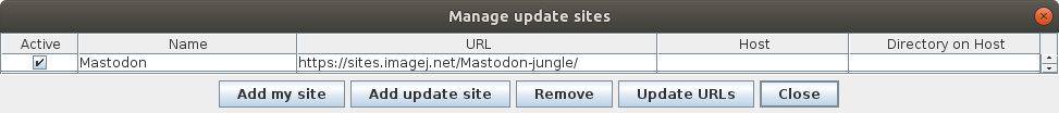 5. Click on the button `Close` in the dialog `Manage update sites`.
6. Click on the button `Apply changes` in the dialog `ImageJ Updater`.
7. Replace `Fiji.app/jars/elephant-0.3.1.jar` with [elephant-0.4.0-SNAPSHOT.jar](https://github.com/elephant-track/elephant-client/releases/download/v0.4.0-dev/elephant-0.4.0-SNAPSHOT.jar)
8. Restart [Fiji](https://imagej.net/software/fiji/).
| Info
5. Click on the button `Close` in the dialog `Manage update sites`.
6. Click on the button `Apply changes` in the dialog `ImageJ Updater`.
7. Replace `Fiji.app/jars/elephant-0.3.1.jar` with [elephant-0.4.0-SNAPSHOT.jar](https://github.com/elephant-track/elephant-client/releases/download/v0.4.0-dev/elephant-0.4.0-SNAPSHOT.jar)
8. Restart [Fiji](https://imagej.net/software/fiji/).
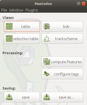
| Info 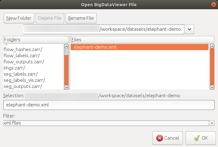 Now, you will see the main window as shown below.
 #### 3. Save & load a Mastodon project
To save the project, you can either run `File > Save Project`, click the `save`/`save as...` button in the main window, or use the shortcut `S`, generate a `.mastodon` file.
A `.mastodon` project file can be loaded by running `File > Load Project` or clicking the `open Mastodon project` button in the `Mastodon launcher` window.
### Setting up the ELEPHANT Server
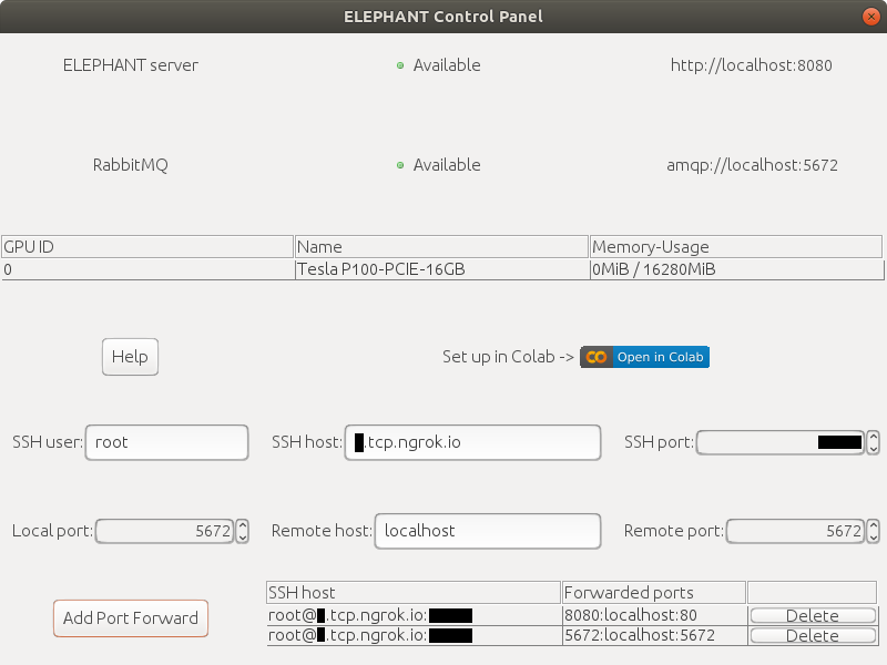
The `Control Panel` is displayed by default at startup. If you cannot find it, run `Plugins > ELEPHANT > Window > Control Panel` to show it.
The `Control Panel` shows the statuses of the servers (ELEPHANT server and [RabbitMQ server](https://www.rabbitmq.com/)).\
It also provides functions for setting up the servers.
| Info
#### 3. Save & load a Mastodon project
To save the project, you can either run `File > Save Project`, click the `save`/`save as...` button in the main window, or use the shortcut `S`, generate a `.mastodon` file.
A `.mastodon` project file can be loaded by running `File > Load Project` or clicking the `open Mastodon project` button in the `Mastodon launcher` window.
### Setting up the ELEPHANT Server
The `Control Panel` is displayed by default at startup. If you cannot find it, run `Plugins > ELEPHANT > Window > Control Panel` to show it.
The `Control Panel` shows the statuses of the servers (ELEPHANT server and [RabbitMQ server](https://www.rabbitmq.com/)).\
It also provides functions for setting up the servers.
| Info 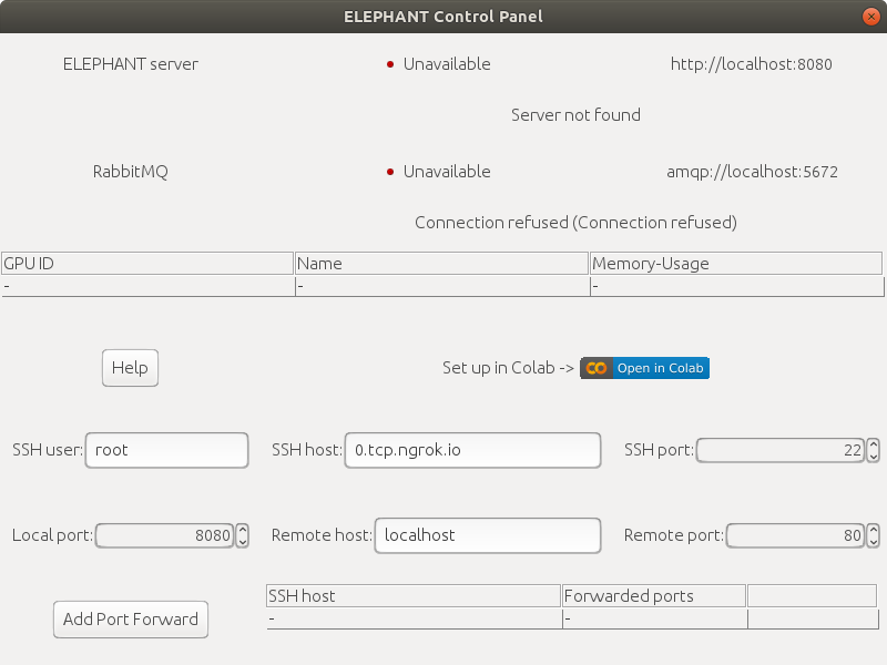 Here, we will set up the servers using [Google Colab](https://research.google.com/colaboratory/faq.html), a freely available product from Google Research. You don't need to have a high-end GPU or a Linux machine to start using ELEPHANT's deep learning capabilities.
#### Setting up with Google Colab
##### 1. Prepare a Google account
If you already have one, you can just use it. Otherwise, create a Google account [here](https://accounts.google.com/signup).
##### 2. Create a ngrok account
Create a ngrok account from the following link.
[ngrok - secure introspectable tunnels to localhost](https://dashboard.ngrok.com/signup)
| Info
Here, we will set up the servers using [Google Colab](https://research.google.com/colaboratory/faq.html), a freely available product from Google Research. You don't need to have a high-end GPU or a Linux machine to start using ELEPHANT's deep learning capabilities.
#### Setting up with Google Colab
##### 1. Prepare a Google account
If you already have one, you can just use it. Otherwise, create a Google account [here](https://accounts.google.com/signup).
##### 2. Create a ngrok account
Create a ngrok account from the following link.
[ngrok - secure introspectable tunnels to localhost](https://dashboard.ngrok.com/signup)
| Info  | Info
 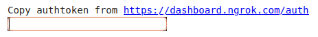 Click the link to open your ngrok account page and copy your authtoken, then paste it to the box above.
 After inputting your authtoken, you will have many lines of outputs. Scroll up and find the following two lines.
```Colab
*** SSH information ***
SSH user: root SSH host: [your_random_value].tcp.ngrok.io SSH port: [your_random_5digits]
Root password: [your_random_password]
```
##### 5. Establish connections from your computer to the servers on Colab
Go back to the `Control Panel` and change the values of `SSH host` and `SSH port` according to the output from Colab. You can leave other fields as default.\
Click the `Add Port Forward` button to establish the connection to the ELEPHANT server. Click `yes` for a warning dialog and enter your password shown on Colab when asked for it.\
Subsequently, change `Local port` to `5672` and `Remote port` to `5672` and click the `Add Port Forward` button to the RabbitMQ server.
If everything is ok, you will see green signals in the `Control Panel`.
After inputting your authtoken, you will have many lines of outputs. Scroll up and find the following two lines.
```Colab
*** SSH information ***
SSH user: root SSH host: [your_random_value].tcp.ngrok.io SSH port: [your_random_5digits]
Root password: [your_random_password]
```
##### 5. Establish connections from your computer to the servers on Colab
Go back to the `Control Panel` and change the values of `SSH host` and `SSH port` according to the output from Colab. You can leave other fields as default.\
Click the `Add Port Forward` button to establish the connection to the ELEPHANT server. Click `yes` for a warning dialog and enter your password shown on Colab when asked for it.\
Subsequently, change `Local port` to `5672` and `Remote port` to `5672` and click the `Add Port Forward` button to the RabbitMQ server.
If everything is ok, you will see green signals in the `Control Panel`.
 ##### 6. Terminate
When you finish using the ELEPHANT, stop and terminate your Colab runtime so that you can release your resources.
- Stop the running execution by `Runtime > Interrupt execution`
- Terminate the runtime by `Runtime > Manage sessions`
##### 6. Terminate
When you finish using the ELEPHANT, stop and terminate your Colab runtime so that you can release your resources.
- Stop the running execution by `Runtime > Interrupt execution`
- Terminate the runtime by `Runtime > Manage sessions`
 | Info
  | Info
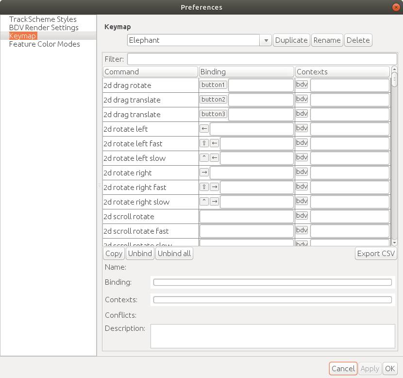
 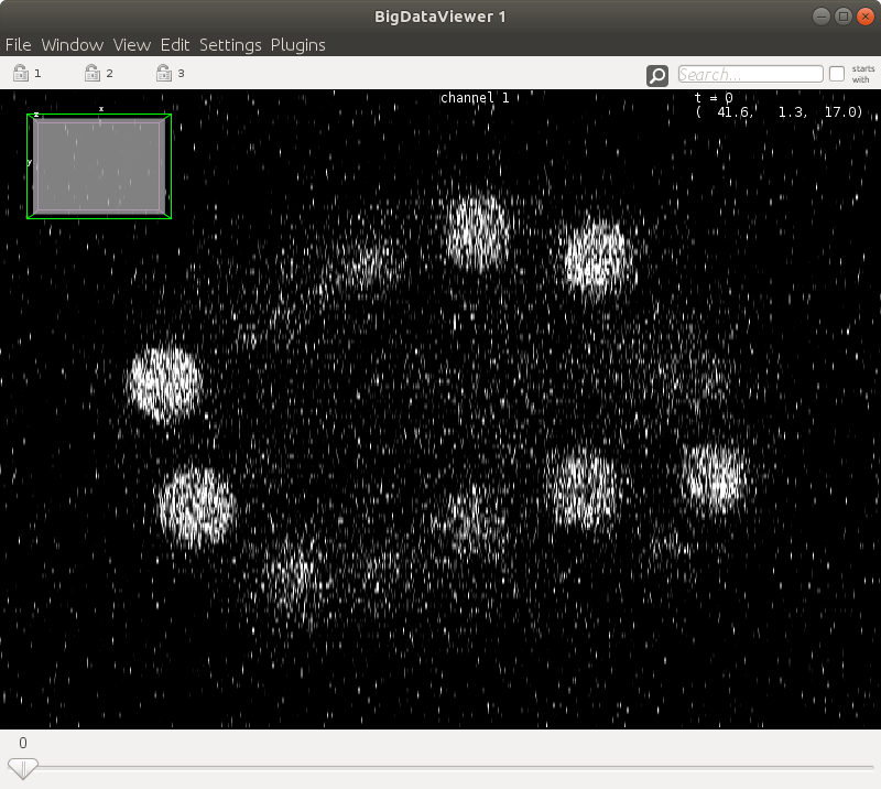 #### 2. Shortcuts
ELEPHANT inherits the user-friendly [shortcuts](https://github.com/mastodon-sc/mastodon#actions-and-keyboard-shortcuts) from Mastodon. To follow this documentation, please find the `Keymap` tab from `File > Preferences...` and select the `Elephant` keymap from the pull down list.
#### 2. Shortcuts
ELEPHANT inherits the user-friendly [shortcuts](https://github.com/mastodon-sc/mastodon#actions-and-keyboard-shortcuts) from Mastodon. To follow this documentation, please find the `Keymap` tab from `File > Preferences...` and select the `Elephant` keymap from the pull down list.
 The following table summaraizes the frequently-used actions used in the BDV window.
| Info
The following table summaraizes the frequently-used actions used in the BDV window.
| Info 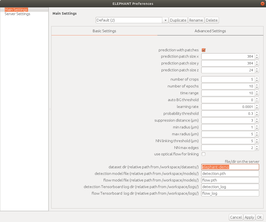 Change the dataset name to `elephant-demo` (or the name you specified for your dataset).
When you change some value in the settings, a new setting profile is created automatically.
| Info
Change the dataset name to `elephant-demo` (or the name you specified for your dataset).
When you change some value in the settings, a new setting profile is created automatically.
| Info 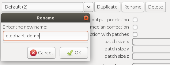 Press the `Apply` button on bottom right and close the settings dialog (`OK` or `x` button on top right).
Please check the settings parameters table for detailed descriptions about the parameters.
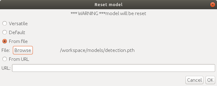
#### 2. Initialize a model
First, you need to initialize a model by `Plugins > ELEPHANT > Detection > Reset Detection Model`.
This command creates a new model parameter file with the name you specified in the settings (`detection.pth` by default) in the `workspace/models/` directory, which lies in the directory you launched on the server.
There are three options for initialization:
1. `Versatile`: initialize a model with a versatile pre-trained model
2. `Default`: initialize a model with intensity-based self-supervised training
3. `From File`: initialize a model from a local file
4. `From URL`: initialize a model from a specified URL
| Info
Press the `Apply` button on bottom right and close the settings dialog (`OK` or `x` button on top right).
Please check the settings parameters table for detailed descriptions about the parameters.
#### 2. Initialize a model
First, you need to initialize a model by `Plugins > ELEPHANT > Detection > Reset Detection Model`.
This command creates a new model parameter file with the name you specified in the settings (`detection.pth` by default) in the `workspace/models/` directory, which lies in the directory you launched on the server.
There are three options for initialization:
1. `Versatile`: initialize a model with a versatile pre-trained model
2. `Default`: initialize a model with intensity-based self-supervised training
3. `From File`: initialize a model from a local file
4. `From URL`: initialize a model from a specified URL
| Info  #### 4. Training on batch mode
Based on the prediction results, you can add annotations as described earlier.
#### 4. Training on batch mode
Based on the prediction results, you can add annotations as described earlier.
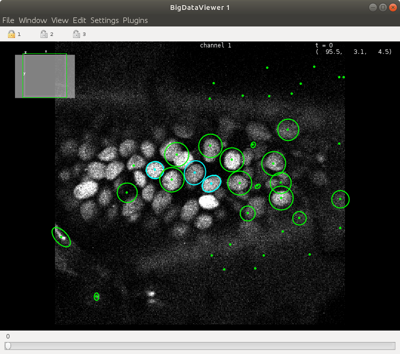 Train the model by `Plugins > ELEPHANT > Detection > Train Selected Timpepoints`.
Predictions with the updated model should yield better results.
Train the model by `Plugins > ELEPHANT > Detection > Train Selected Timpepoints`.
Predictions with the updated model should yield better results.
 In general, a batch mode is used for training with relatively large amounts of data. For more interactive training, please use the live mode explained below.
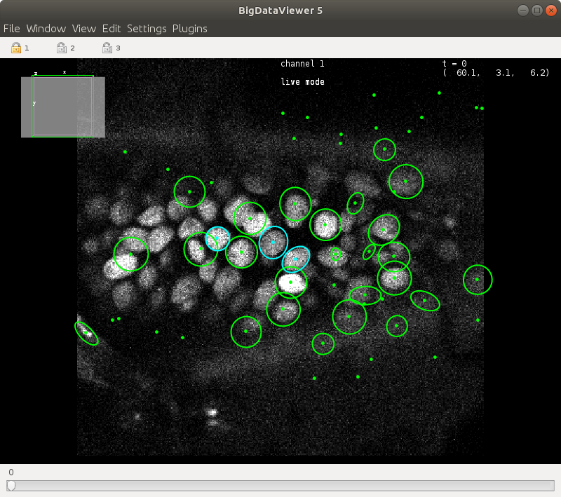
#### 5. Training on live mode
In live mode, you can iterate the cycles of annotation, training, prediction and proofreading more frequently.
Start live mode by `Plugins > ELEPHANT > Detection > Live Training`.
During live mode, you can find the text "live mode" on top of the BDV view.
In general, a batch mode is used for training with relatively large amounts of data. For more interactive training, please use the live mode explained below.
#### 5. Training on live mode
In live mode, you can iterate the cycles of annotation, training, prediction and proofreading more frequently.
Start live mode by `Plugins > ELEPHANT > Detection > Live Training`.
During live mode, you can find the text "live mode" on top of the BDV view.
 Every time you update the labels (Shortcut: `U`), a new training epoch will start, with the latest labels in the current timepoint.
To perform prediction with the latest model, the user needs to run `Predict Spots` (Shortcut: `Alt`+`S`) after the model is updated.
#### 6. Saving a model
The model parameter files are located under `workspace/models` on the server.\
If you are using your local machine as a server, these files should remain unless you do not delete them explicitly.\
If you are using Google Colab, you may need to save them before terminating the session.\
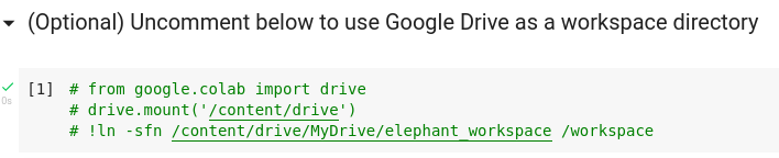
You can download the model parameter file by running `Plugins > ELEPHANT > Detection > Download Detection Model` or `Plugins > ELEPHANT > Linking > Download Flow Model`.\
Alternatively, you can make it persistent on your Google drive by uncommenting the first code cell in the Colab notebook.
Every time you update the labels (Shortcut: `U`), a new training epoch will start, with the latest labels in the current timepoint.
To perform prediction with the latest model, the user needs to run `Predict Spots` (Shortcut: `Alt`+`S`) after the model is updated.
#### 6. Saving a model
The model parameter files are located under `workspace/models` on the server.\
If you are using your local machine as a server, these files should remain unless you do not delete them explicitly.\
If you are using Google Colab, you may need to save them before terminating the session.\
You can download the model parameter file by running `Plugins > ELEPHANT > Detection > Download Detection Model` or `Plugins > ELEPHANT > Linking > Download Flow Model`.\
Alternatively, you can make it persistent on your Google drive by uncommenting the first code cell in the Colab notebook.
 You can find [pretrained parameter files](https://github.com/elephant-track/elephant-server/releases/tag/data) used in the paper.
#### 7. Importing a model
The model parameter file can be specified in the `Preferences` dialog, where the file path is relative to `/workspace/models/` on the server.\
There are three ways to import the pre-trained model parameters:
1. Run `Plugins > ELEPHANT > Detection > Reset Detection Model` and select the `From File` option with the local file.
You can find [pretrained parameter files](https://github.com/elephant-track/elephant-server/releases/tag/data) used in the paper.
#### 7. Importing a model
The model parameter file can be specified in the `Preferences` dialog, where the file path is relative to `/workspace/models/` on the server.\
There are three ways to import the pre-trained model parameters:
1. Run `Plugins > ELEPHANT > Detection > Reset Detection Model` and select the `From File` option with the local file.
 2. Upload the pre-trained parameters file to the website that provides a public download URL (e.g. GitHub, Google Drive, Dropbox). Run `Plugins > ELEPHANT > Detection > Reset Detection Model` and select the `From URL` option with the download URL.
 3. Directly place/replace the file at the specified file path on the server.
### Linking workflow
| Info
3. Directly place/replace the file at the specified file path on the server.
### Linking workflow
| Info 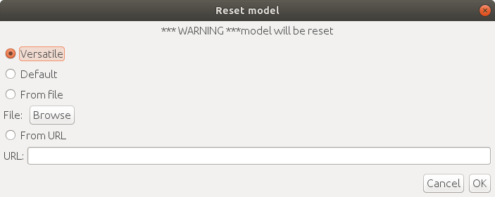 Run the nearest neighbor linking action by `Alt`+`L` or `Plugins > ELEPHANT > Linking > Nearest Neighbor Linking`.
#### 5. Proofreading
Using both the BDV window and the trackscheme, you can remove/add/modify spots and links to build a complete lineage tree.
Once you finish proofreading of a track (or a tracklet), you can tag it as `Approved` in the `Tracking` tag set.
Select all spots and links in the track by `Shift`+`Space`, and `Edit > Tags > Tracking > Approved`. There is a set of shortcuts to perform tagging efficiently. The shortcut `Y` pops up a small window on top left in the TrackScheme window, where you can select the tag set, followed by the tag by pressing a number in the list. For example, `Edit > Tags > Tracking > Approved` corresponds to the set of shortcuts [`Y` > `2` > `1`].
Spots and links tagged with `Approved` will remain unless users do not reomove them explicitly (the `unlabeled` links will be removed at the start of the next prediction). The `Approved` links will also be used for training of a flow model.
| Info
Run the nearest neighbor linking action by `Alt`+`L` or `Plugins > ELEPHANT > Linking > Nearest Neighbor Linking`.
#### 5. Proofreading
Using both the BDV window and the trackscheme, you can remove/add/modify spots and links to build a complete lineage tree.
Once you finish proofreading of a track (or a tracklet), you can tag it as `Approved` in the `Tracking` tag set.
Select all spots and links in the track by `Shift`+`Space`, and `Edit > Tags > Tracking > Approved`. There is a set of shortcuts to perform tagging efficiently. The shortcut `Y` pops up a small window on top left in the TrackScheme window, where you can select the tag set, followed by the tag by pressing a number in the list. For example, `Edit > Tags > Tracking > Approved` corresponds to the set of shortcuts [`Y` > `2` > `1`].
Spots and links tagged with `Approved` will remain unless users do not reomove them explicitly (the `unlabeled` links will be removed at the start of the next prediction). The `Approved` links will also be used for training of a flow model.
| Info | Category | Action | On Menu | Shortcut | Description | |
|---|---|---|---|---|---|
| Detection | Predict Spots | Yes | Alt+S |
Predict spots with the specified model and parameters | |
| Predict Spots Around Mouse | No | Alt+Shift |
Predict spots around the mouse position on the BDV view | ||
| Update Detection Labels | Yes | U |
Predict spots | ||
| Reset Detection Labels | Yes | Not available | Reset detection labels | ||
| Start Live Training | Yes | Not available | Start live training | ||
| Train Detection Model (Selected Timepoints) | Yes | Not available | Train a detection model with the annotated data from the specified timepoints | ||
| Train Detection Model (All Timepoints) | Yes | Not available | Train a detection model with the annotated data from all timepoints | ||
| Reset Detection Model | Yes | Not available | Reset a detection model by one of the following modes: `Versatile`, `Default`, `From File` or `From URL` | ||
| Download Detection Model | Yes | Not available | Download a detection model parameter file. | ||
| Linking | Nearest Neighbor Linking | Yes | Alt+L |
Perform nearest neighbor linking with the specified model and parameters | |
| Nearest Neighbor Linking Around Mouse | No | Alt+Shift+L |
Perform nearest neighbor linking around the mouse position on the BDV view | ||
| Update Flow Labels | Yes | Not available | Update flow labels | ||
| Reset Flow Labels | Yes | Not available | Reset flow labels | ||
| Train Flow Model (Selected Timepoints) | Yes | Not available | Train a flow model with the annotated data from the specified timepoints | ||
| Reset Flow Model | Yes | Not available | Reset a flow model by one of the following modes: `Versatile`, `Default`, `From File` or `From URL` | ||
| Download Flow Model | Yes | Not available | Download a flow model parameter file. | ||
| Utils | Map Spot Tag | Yes | Not available | Map a spot tag to another spot tag | |
| Map Link Tag | Yes | Not available | Map a link tag to another link tag | ||
| Remove All Spots and Links | Yes | Not available | Remove all spots and links | ||
| Remove Short Tracks | Yes | Not available | Remove spots and links in the tracks that are shorter than the specified length | ||
| Remove Spots by Tag | Yes | Not available | Remove spots with the specified tag | ||
| Remove Links by Tag | Yes | Not available | Remove spots with the specified tag | ||
| Remove Visible Spots | Yes | Not available | Remove spots in the current visible area for the specified timepoints | ||
| Remove Self Links | Yes | Not available | Remove accidentally generated links that connect the identical spots | ||
| Take a Snapshot | Yes | H |
Take a snapshot in the specified BDV window | ||
| Take a Snapshot Movie | Yes | Not available | Take a snapshot movie in the specified BDV window | ||
| Import Mastodon | Yes | Not available | Import spots and links from a .mastodon file. |
||
| Export CTC | Yes | Not available | Export tracking results in a Cell Tracking Challenge format. The tracks whose root spots are tagged with Completed are exported. |
||
| Change Detection Tag Set Colors | Yes | Not available | Change Detection tag set colors (Basic or Advanced) |
||
| Analysis | Tag Progenitors | Yes | Not available | Assign the Progenitor tags to the tracks whose root spots are tagged with Completed. Tags are automatically assigned starting from 1. Currently, this action supports maximum 255 tags. |
|
| Tag Progenitors | Yes | Not available | Label the tracks with the following rule.
|
||
| Tag Dividing Cells | Yes | Not available | Tag the dividing and divided spots in the tracks as below.
|
||
| Count Divisions (Entire) | Yes | Not available | Count number of divisions in a lineage tree and output as a .csv file. In the Entire mode, a total number of divisions per timepoint is calculated.In the Trackwise mode, a trackwise number of divisions per timepoint is calculated. |
||
| Count Divisions (Trackwise) | |||||
| Window | Client Log | Yes | Not available | Show a client log window | |
| Server Log | Yes | Not available | Show a server log window | ||
| Control Panel | Yes | Not available | Show a control panel window | ||
| Abort Processing | Yes | Ctrl+C |
Abort the current processing | ||
| Preferences... | Yes | Not available | Open a preferences dialog | ||
 Predicted spots and manually added spots are tagged by default as `unlabeled` and `fn`, respectively.
These tags are used for training, where **true** spots and **false** spots can have different weights for training.
Highlighted spots can be tagged with one of the `Detection` tags using the shortcuts shown below.
| Tag | Shortcut |
| --------- | -------- |
| tp | 4 |
| fp | 5 |
| tn | 6 |
| fn | 7 |
| tb | 8 |
| fb | 9 |
| unlabeled | 0 |
## Tag sets available on ELEPHANT
By default, ELEPHANT generates and uses the following tag sets.
Predicted spots and manually added spots are tagged by default as `unlabeled` and `fn`, respectively.
These tags are used for training, where **true** spots and **false** spots can have different weights for training.
Highlighted spots can be tagged with one of the `Detection` tags using the shortcuts shown below.
| Tag | Shortcut |
| --------- | -------- |
| tp | 4 |
| fp | 5 |
| tn | 6 |
| fn | 7 |
| tb | 8 |
| fb | 9 |
| unlabeled | 0 |
## Tag sets available on ELEPHANT
By default, ELEPHANT generates and uses the following tag sets.
| Tag set | Tag | Color | Description | |
|---|---|---|---|---|
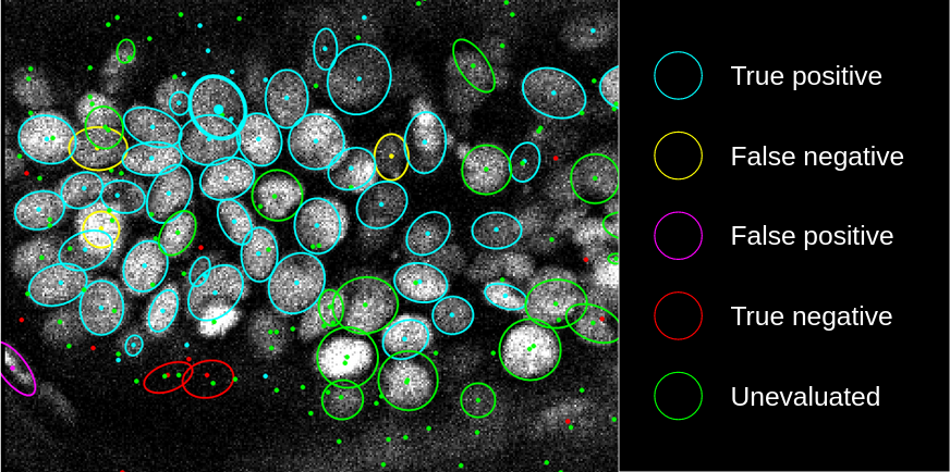
| Detection | tp | ■ cyan | Annotate spots for training and prediction in a detection workflow |
true positive; generates nucleus center and nucleus periphery labels |
| fp | ■ magenta | false positive; generates background labels with a false weight | ||
| tn | ■ red | true negative; generates background labels | ||
| fn | ■ yellow | false negative; generates nucleus center and nucleus periphery labels with a false weight | ||
| tb | ■ orange | true border; generates nucleus periphery labels | ||
| fb | ■ pink | false border; generates nucleus periphery labels with a false weight | ||
| unlabeled | ■ green | unevaluated; not used for labels | ||
| Tracking | Approved | ■ cyan | Annotate links for training and prediction in a linking workflow |
approved; generates flow labels |
| unlabeled | ■ green | unevaluated; not used for flow labels | ||
| Progenitor | 1-255 | ■ glasbey | Visualize progenitors | assigned by an anlysis plugin or manually by a user |
| unlabeled | ■ invisible | not assigned; invisible on the view | ||
| Status | Completed | ■ cyan | Label status of tracks | completed tracks |
| Division | Dividing | ■ cyan | Annotate division status of spots |
spots about to divide |
| Divided | ■ yellow | spots just divided | ||
| Non-dividing | ■ magenta | othe positive spots | ||
| Invisible | ■ invisible | negative spots are invisible | ||
| Proliferator | Proliferator | ■ cyan | Annotate proliferation status of spots |
spots in the proliferating lineage tree |
| Non-proliferator | ■ magenta | spots in the non-proliferating lineage tree | ||
| Invisible | ■ invisible | undetermined spots are invisible | ||
| Category | Parameter | Description |
|---|---|---|
| Basic Settings | prediction with patches | If checked, prediction is performed on the patches with the size specified below. |
| patch size x | Patch size for x axis. If the prediction with patches is unchecked, it is not used. |
|
| patch size y | Patch size for y axis. If the prediction with patches is unchecked, it is not used. |
|
| patch size z | Patch size for z axis. If the prediction with patches is unchecked, it is not used. |
|
| number of crops | Number of crops per timepoint per epoch used for training. | |
| number of epochs | Number of epochs for batch training. Ignored in live mode. | |
| time range | Time range (backward) for prediction and batch training. For example, if the current time point is `10` and the specified time range is `5`, time points `[6, 7, 8, 9, 10]` are used for prediction and batch training. | |
| auto BG threshold | Voxels with the normalized value below auto BG threshold are considered as *BG* in the label generation step. |
|
| learning rate | Learning rate for training. | |
| probablility threshold | Voxels with a center probability greater than this threshold are treated as the center of the ellipsoid in detection. | |
| suppression distance | If the predicted spot has an existing spot (either TP, FN or unlabeled) within this value, one of the spots is suppressed.If the existing spot is TP or FN, the predicted spot is suppressed.If the existing spot is unlabeled, the smaller of the two spots is suppressed. |
|
| min radius | If one of the radii of the predicted spot is smaller than this value, the spot will be discarded. | |
| max radius | Radii of the predicted spot is clamped to this value. | |
| NN linking threshold | In the linking workflow, the length of the link should be smaller than this value. If the optical flow is used in linking, the length is calculated as the distance based on the flow-corrected position of the spot. This value is referred to as d_serch in the paper. |
|
| NN max edges | This value determines the number of links allowed to be created in the linking Workflow. | |
| use optical flow for linking | If checked, optical flow estimation is used to support nearest neighbor (NN) linking. | |
| dataset dir | The path of the dataset dir stored on the server. The path is relative to /workspace/models/ on the server. |
|
| detection model file | The path of the [state_dict](https://pytorch.org/tutorials/beginner/saving_loading_models.html#what-is-a-state-dict) file for the detection model stored on the server. The path is relative to /workspace/models/ on the server. |
|
| flow model file | The path of the [state_dict](https://pytorch.org/tutorials/beginner/saving_loading_models.html#what-is-a-state-dict) file for the flow model stored on the server. The path is relative to /workspace/models/ on the server. |
|
| detection Tensorboard log dir | The path of the Tensorboard log dir for the detection model stored on the server. The path is relative to /workspace/logs/ on the server. |
|
| flow Tensorboard log dir | The path of the Tensorboard log dir for the flow model stored on the server. The path is relative to /workspace/logs/ on the server. |
|
| Advanced Settings | output prediction | If checked, prediction output is save as .zarr on the server for the further inspection. |
| apply slice-wise median correction | If checked, the slice-wise median value is shifted to the volume-wise median value. It cancels the uneven slice wise intensity distribution. |
|
| mitigate edge discontinuities | If checked, discontinuities found in the edge regions of the prediction are mitigated. The required memory size will increase slightly. |
|
| training crop size x | Training crop size for x axis. The smaller of this parameter and the x dimension of the image is used for the actual crop size x. | |
| training crop size y | Training crop size for y axis. The smaller of this parameter and the y dimension of the image is used for the actual crop size y. | |
| training crop size z | Training crop size for z axis. The smaller of this parameter and the z dimension of the image is used for the actual crop size z. | |
| class weight bg | Class weight for background in the loss function for the detection model. | |
| class weight border | Class weight for border in the loss function for the detection model. | |
| class weight center | Class weight for center in the loss function for the detection model. | |
| flow dim weight x | Weight for x dimension in the loss function for the flow model. | |
| flow dim weight y | Weight for y dimension in the loss function for the flow model. | |
| flow dim weight z | Weight for z dimension in the loss function for the flow model. | |
| false weight | Labels generated from false annotations (FN, FP, FB) are weighted with this value in loss calculation during training (relative to true annotations). |
|
| center ratio | Center ratio of the ellipsoid used in label generation and detection. | |
| max displacement | Maximum displacement that would be predicted with the flow model. This value is used to scale the output from the flow model. Training and prediction should use the same value for this parameter. If you want to transfer the flow model to another dataset, this value should be kept. |
|
| augmentation scale factor base | In training, the image volume is scaled randomly based on this value. e.g. If this value is 0.2, the scaling factors for three axes are randomly picke up from the range [0.8, 1.2]. |
|
| augmentation rotation angle | In training, the XY plane is randomly rotated based on this value. The unit is degree. e.g. If this value is 30, the rotation angle is randomly picked up from the range [-30, 30]. |
|
| NN search depth | This value determines how many timepoints the algorithm searches for the parent spot in the linking workflow. | |
| NN search neighbors | This value determines how many neighbors are considered as candidates for the parent spot in the linking workflow. | |
| use interpolation for linking | If checked, the missing spots in the link are interpolated, which happens when 1 < NN search neighbors. |
|
| log file basename | This value specifies log file basename.~/.mastodon/logs/client_BASENAME.log, ~/.mastodon/logs/server_BASENAME.log will be created and used as log files. |
|
| Server Settings | ELEPHANT server URL with port number | URL for the ELEPHANT server. It should include the port number (e.g. http://localhost:8080) |
| RabbitMQ server port | Port number of the RabbitMQ server. | |
| RabbitMQ server host name | Host name of the RabbitMQ server. (e.g. localhost) |
|
| RabbitMQ server username | Username for the RabbitMQ server. | |
| RabbitMQ server password | Password for the RabbitMQ server. |
Alternatively, you can use CLI. Assuming that you can access to the computer that launches the ELEPHANT server by `ssh USERNAME@HOSTNAME` (or `ssh.exe USERNAME@HOSTNAME` on Windows), you can forward the ports for ELEPHANT as below.
```bash
ssh -N -L 8080:localhost:8080 USERNAME@HOSTNAME # NGINX
ssh -N -L 5672:localhost:5672 USERNAME@HOSTNAME # RabbitMQ
```
```powershell
ssh.exe -N -L 8080:localhost:8080 USERNAME@HOSTNAME # NGINX
ssh.exe -N -L 5672:localhost:5672 USERNAME@HOSTNAME # RabbitMQ
```
After establishing these connections, the ELEPHANT client can communicate with the ELEPHANT server just as launched on localhost.
## Demo Data
[](https://doi.org/10.5281/zenodo.5519708)
## Acknowledgements
This research was supported by the European Research Council, under the European Union Horizon 2020 programme, grant ERC-2015-AdG #694918. The software is developed in Institut de Génomique Fonctionnelle de Lyon (IGFL) / Centre national de la recherche scientifique (CNRS).
- ELEPHANT client
- [Mastodon](https://github.com/mastodon-sc/mastodon)
- [BigDataViewer](https://github.com/bigdataviewer/bigdataviewer-core)
- [SciJava](https://scijava.org/)
- [Unirest-java](http://kong.github.io/unirest-java/)
- ELEPHANT server
- [PyTorch](https://pytorch.org/)
- [Numpy](https://numpy.org/)
- [Scipy](https://www.scipy.org/)
- [scikit-image](https://scikit-image.org/)
- [Flask](https://flask.palletsprojects.com/en/1.1.x/)
- [uWSGI](https://uwsgi-docs.readthedocs.io/en/latest/)
- [NGINX](https://www.nginx.com/)
- [Redis](https://redis.io/)
- [RabbitMQ](https://www.rabbitmq.com/)
- [Supervisord](http://supervisord.org/)
- [uwsgi-nginx-flask-docker](https://github.com/tiangolo/uwsgi-nginx-flask-docker)
- [ngrok](https://ngrok.com/)
- [Google Colab](https://colab.research.google.com)
- ELEPHANT docs
- [Docsify](https://docsify.js.org)
and other great projects.
## Contact
[Ko Sugawara](http://www.ens-lyon.fr/lecole/nous-connaitre/annuaire/ko-sugawara)
Please post feedback and questions to the [Image.sc forum](https://forum.image.sc/tag/elephant).\
It is important to add the tag `elephant` to your posts so that we can reach you quickly.
## Citation
Please cite our paper on [eLife](https://doi.org/10.7554/eLife.69380).
- Sugawara, K., Çevrim, C. & Averof, M. [*Tracking cell lineages in 3D by incremental deep learning.*](https://doi.org/10.7554/eLife.69380) eLife 2022. doi:10.7554/eLife.69380
```.bib
@article {Sugawara2022,
author = {Sugawara, Ko and {\c{C}}evrim, {\c{C}}a?r? and Averof, Michalis},
title = {Tracking cell lineages in 3D by incremental deep learning},
year = {2022},
doi = {10.7554/eLife.69380},
abstract = {Deep learning is emerging as a powerful approach for bioimage analysis. Its use in cell tracking is limited by the scarcity of annotated data for the training of deep-learning models. Moreover, annotation, training, prediction, and proofreading currently lack a unified user interface. We present ELEPHANT, an interactive platform for 3D cell tracking that addresses these challenges by taking an incremental approach to deep learning. ELEPHANT provides an interface that seamlessly integrates cell track annotation, deep learning, prediction, and proofreading. This enables users to implement cycles of incremental learning starting from a few annotated nuclei. Successive prediction-validation cycles enrich the training data, leading to rapid improvements in tracking performance. We test the software's performance against state-of-the-art methods and track lineages spanning the entire course of leg regeneration in a crustacean over 1 week (504 time-points). ELEPHANT yields accurate, fully-validated cell lineages with a modest investment in time and effort.},
URL = {https://doi.org/10.7554/eLife.69380},
journal = {eLife}
}
```
## License
[BSD-2-Clause](_LICENSE.md)
