{
"cells": [
{
"cell_type": "markdown",
"metadata": {},
"source": [
"| [Table of Contents](#table_of_contents) | [Data and model](#data_and_model) | [Natural estimators](#natural_estimators) | [NN-DOOLSE, MLE](#doolse) | [NN-MDOOLSE, REMLE](#mdoolse) | [References](#references) |"
]
},
{
"cell_type": "markdown",
"metadata": {},
"source": [
"**Authors:** Jozef Hanč, Martina Hančová, Andrej Gajdoš
*[Faculty of Science](https://www.upjs.sk/en/faculty-of-science/?prefferedLang=EN), P. J. Šafárik University in Košice, Slovakia*
emails: [martina.hancova@upjs.sk](mailto:martina.hancova@upjs.sk)\n",
"***\n",
"** EBLUP-NE for tourism** "
]
},
{
"cell_type": "markdown",
"metadata": {},
"source": [
" Python-based computational tools - **SciPy, CVXPY** \n",
"\n",
"### Table of Contents \n",
"* [Data and model](#data_and_model) - data and model description of empirical data\n",
"* [Natural estimators](#natural_estimators) - EBLUPNE based on NE\n",
"* [NN-DOOLSE, MLE](#doolse) - EBLUPNE based on nonnegative DOOLSE (same as MLE)\n",
"* [NN-MDOOLSE, REMLE](#mdoolse) - EBLUPNE based on nonnegative MDOOLSE (same as REMLE)\n",
"* [References](#references)\n",
"\n",
"**To get back to the contents, use the Home key.**"
]
},
{
"cell_type": "markdown",
"metadata": {},
"source": [
"## Python libraries"
]
},
{
"cell_type": "markdown",
"metadata": {},
"source": [
"## CVXPY: A Python-Embedded Modeling Language for Convex Optimization \n",
"\n",
"* _Purpose_: scientific Python library for solving convex optimization tasks\n",
"* _Version_: 1.0.1, 2018\n",
"* _URL_: https://www.cvxpy.org/\n",
"* _Computational parameters_ of CVXPY:\n",
"> * *solver* - the convex optimization solver ECOS, OSQP, and SCS chosen according to the given problem\n",
" * **OSQP** for convex quadratic problems\n",
" * `max_iter` - maximum number of iterations (default: 10000).\n",
" * `eps_abs` - absolute accuracy (default: 1e-4).\n",
" * `eps_rel` - relative accuracy (default: 1e-4).\n",
" * **ECOS** for convex second-order cone problems \n",
" * `max_iters` - maximum number of iterations (default: 100).\n",
" * `abstol` - absolute accuracy (default: 1e-7).\n",
" * `reltol` - relative accuracy (default: 1e-6).\n",
" * `feastol` - tolerance for feasibility conditions (default: 1e-7).\n",
" * `abstol_inacc` - absolute accuracy for inaccurate solution (default: 5e-5).\n",
" * `reltol_inacc` - relative accuracy for inaccurate solution (default: 5e-5).\n",
" * `feastol_inacc` - tolerance for feasibility condition for inaccurate solution (default: 1e-4).\n",
" * **SCS** for large-scale convex cone problems\n",
" * `max_iters` - maximum number of iterations (default: 2500).\n",
" * `eps` - convergence tolerance (default: 1e-4).\n",
" * `alpha` - relaxation parameter (default: 1.8).\n",
" * `scale` - balance between minimizing primal and dual residual (default: 5.0).\n",
" * `normalize` - whether to precondition data matrices (default: True).\n",
" * `use_indirect` - whether to use indirect solver for KKT sytem (instead of direct) (default: True)."
]
},
{
"cell_type": "markdown",
"metadata": {},
"source": [
"## Scipy - NumPy, Pandas\n",
"* Numpy is the fundamental Python library of SciPy ecosystem for fast scientific computing with large, multi-dimensional arrays and matrices, along with a large collection of high-level mathematical functions to operate on these arrays. \n",
"* default precision: double floating-point precision $\\text{eps}<10^{-15}$\n",
"* Pandas is the Python library providing high-performance, easy to use data structures."
]
},
{
"cell_type": "code",
"execution_count": 1,
"metadata": {
"ExecuteTime": {
"end_time": "2019-05-12T14:02:09.989000Z",
"start_time": "2019-05-12T14:02:09.214000Z"
}
},
"outputs": [],
"source": [
"import cvxpy\n",
"import numpy as np\n",
"import pandas as pd\n",
"import platform as pt\n",
"\n",
"from cvxpy import *\n",
"from math import cos, sin\n",
"from numpy.linalg import inv, norm\n",
"from itertools import product\n",
"from __future__ import print_function\n",
"from __future__ import division\n",
"\n",
"np.set_printoptions(precision=10)"
]
},
{
"cell_type": "code",
"execution_count": 2,
"metadata": {
"ExecuteTime": {
"end_time": "2019-05-12T14:02:10.004000Z",
"start_time": "2019-05-12T14:02:09.992000Z"
},
"scrolled": true
},
"outputs": [
{
"name": "stdout",
"output_type": "stream",
"text": [
"cvxpy:1.0.1\n",
"numpy:1.14.5\n",
"pandas:0.23.4\n",
"python:2.7.15\n"
]
}
],
"source": [
"# software versions\n",
"print('cvxpy:'+cvxpy.__version__)\n",
"print('numpy:'+np.__version__)\n",
"print('pandas:'+pd.__version__)\n",
"print('python:'+pt.python_version())"
]
},
{
"cell_type": "markdown",
"metadata": {},
"source": [
"***\n",
"\n",
"# Data and model "
]
},
{
"cell_type": "markdown",
"metadata": {},
"source": [
"In this econometric FDSLRM application, we consider the time series data set, called \n",
"`visnights`, representing *total quarterly visitor nights* (in millions) from \n",
"1998-2016 in one of the regions of Australia -- inner zone of Victoria state. The number of time \n",
"series observations is $n=76$. The data was adapted from _Hyndman, 2018_.\n",
"\n",
"The Gaussian orthogonal FDSLRM fitting the tourism data has the following form:\n",
"\n",
"$ \n",
"\\begin{array}{rl}\n",
"& X(t) & \\! = \\! & \\beta_1+\\beta_2\\cos\\left(\\tfrac{2\\pi t}{76}\\right)+\\beta_3\\sin\\left(\\tfrac{2\\pi t\\cdot 2}{76}\\right) + \\\\\n",
"& & & +Y_1\\cos\\left(\\tfrac{2\\pi t\\cdot 19 }{76}\\right)+Y_2\\sin\\left(\\tfrac{2\\pi t\\cdot 19}{76}\\right) +Y_3\\cos\\left(\\tfrac{2\\pi t\\cdot 38}{76}\\right) +w(t), \\, t\\in \\mathbb{N},\n",
"\\end{array}\n",
"$ \n",
"\n",
"where $\\boldsymbol{\\beta}=(\\beta_1,\\,\\beta_2,\\,\\beta_3)' \\in \\mathbb{R}^3, \\mathbf{Y} = (Y_1, Y_2, Y_3)' \\sim \\mathcal{N}_3(\\boldsymbol{0}, \\mathrm{D}), w(t) \\sim \\mathcal{iid}\\, \\mathcal{N} (0, \\sigma_0^2), \\boldsymbol{\\nu}=(\\sigma_0^2, \\sigma_1^2, \\sigma_2^2, \\sigma_3^2) \\in \\mathbb{R}_{+}^4$.\n",
"\n",
"We identified the given and most parsimonious structure of the FDSLRM using an iterative process of the model building and selection based on exploratory tools of *spectral analysis* and *residual diagnostics* (for details see our Jupyter notebook `tourism.ipynb`)."
]
},
{
"cell_type": "markdown",
"metadata": {},
"source": [
"## SciPy(Numpy)"
]
},
{
"cell_type": "code",
"execution_count": 3,
"metadata": {
"ExecuteTime": {
"end_time": "2019-05-12T14:02:10.040000Z",
"start_time": "2019-05-12T14:02:10.009000Z"
}
},
"outputs": [
{
"data": {
"text/plain": [
"(76L, 1L)"
]
},
"execution_count": 3,
"metadata": {},
"output_type": "execute_result"
}
],
"source": [
"# data - time series observation\n",
"path = 'tourism.csv'\n",
"data = pd.read_csv(path, sep=';', usecols=[1])\n",
"\n",
"# observation x as matrix\n",
"x = np.asmatrix(data.values)\n",
"x.shape"
]
},
{
"cell_type": "code",
"execution_count": 4,
"metadata": {
"ExecuteTime": {
"end_time": "2019-05-12T14:02:10.064000Z",
"start_time": "2019-05-12T14:02:10.046000Z"
}
},
"outputs": [],
"source": [
"# model parameters\n",
"n, k, l = 76, 3, 3\n",
"\n",
"# significant frequencies\n",
"om1, om2, om3, om4 = 2*np.pi/76, 2*np.pi*2/76, 2*np.pi*19/76, 2*np.pi*38/76\n",
"\n",
"# model - design matrices F', F, V',V\n",
"Fc = np.mat([[1 for t in range(1,n+1)],\n",
" [cos(om1*t) for t in range(1,n+1)],\n",
" [sin(om2*t) for t in range(1,n+1)]])\n",
"Vc = np.mat([[cos(om3*t) for t in range(1,n+1)],\n",
" [sin(om3*t) for t in range(1,n+1)],\n",
" [cos(om4*t) for t in range(1,n+1)]])\n",
"F, V = Fc.T, Vc.T\n",
"\n",
"# columns vj of V and their squared norm ||vj||^2\n",
"vv = lambda j: V[:,j-1]\n",
"nv2 = lambda j: np.trace(vv(j).T*vv(j))"
]
},
{
"cell_type": "code",
"execution_count": 5,
"metadata": {
"ExecuteTime": {
"end_time": "2019-05-12T14:02:10.087000Z",
"start_time": "2019-05-12T14:02:10.070000Z"
}
},
"outputs": [],
"source": [
"# auxiliary matrices and vectors\n",
"\n",
"# Gram matrices GF, GV\n",
"GF, GV = Fc*F, Vc*V\n",
"InvGF, InvGV = inv(GF), inv(GV)\n",
"\n",
"# projectors PF, MF, PV, MV\n",
"In = np.identity(n)\n",
"PF = F*InvGF*Fc\n",
"PV = V*InvGV*Vc\n",
"MF, MV = In-PF, In-PV\n",
"\n",
"# residuals e, e'\n",
"e = MF*x\n",
"ec = e.T"
]
},
{
"cell_type": "code",
"execution_count": 6,
"metadata": {
"ExecuteTime": {
"end_time": "2019-05-12T14:02:10.103000Z",
"start_time": "2019-05-12T14:02:10.091000Z"
}
},
"outputs": [
{
"data": {
"text/plain": [
"(matrix([[ 3.5527136788e-15, -1.0658141036e-14, 0.0000000000e+00],\n",
" [ 7.6265746656e-15, -2.2367944157e-15, 1.9984014443e-15],\n",
" [ 7.6719645096e-15, -5.5627717914e-15, -4.6210314404e-16]]),\n",
" matrix([[ 3.8000000000e+01, -5.5047207898e-16, -3.2196467714e-15],\n",
" [-5.5047207898e-16, 3.8000000000e+01, -9.3258734069e-15],\n",
" [-3.2196467714e-15, -9.3258734069e-15, 7.6000000000e+01]]))"
]
},
"execution_count": 6,
"metadata": {},
"output_type": "execute_result"
}
],
"source": [
"# orthogonality condition\n",
"Fc*V, GV"
]
},
{
"cell_type": "markdown",
"metadata": {},
"source": [
"***\n",
"\n",
"# Natural estimators\n",
"\n",
"## ANALYTICALLY \n",
"using formula (4.1) from _Hancova et al 2019_\n",
"\n",
">$\n",
"\\renewcommand{\\arraystretch}{1.4}\n",
"\\breve{\\boldsymbol{\\nu}}(\\mathbf{e}) =\n",
"\\begin{pmatrix}\n",
"\\tfrac{1}{n-k-l}\\,\\mathbf{e}'\\,\\mathrm{M_V}\\,\\mathbf{e} \\\\\n",
"(\\mathbf{e}'\\mathbf{v}_1)^2/||\\mathbf{v}_1||^4 \\\\\n",
"\\vdots \\\\\n",
"(\\mathbf{e}'\\mathbf{v}_l)^2/||\\mathbf{v}_l||^4\n",
"\\end{pmatrix} \n",
"$\n",
"\n",
"## $\\boldsymbol{1^{st}}$ stage of EBLUP-NE "
]
},
{
"cell_type": "markdown",
"metadata": {},
"source": [
"## SciPy(Numpy)"
]
},
{
"cell_type": "code",
"execution_count": 7,
"metadata": {
"ExecuteTime": {
"end_time": "2019-05-12T14:02:10.116000Z",
"start_time": "2019-05-12T14:02:10.107000Z"
}
},
"outputs": [
{
"name": "stdout",
"output_type": "stream",
"text": [
"[0.10766780139512397, 0.0039056202882091925, 0.23030624879955963, 0.02227313104780322] 0.25523453906141463\n"
]
}
],
"source": [
"# NE according to formula (4.1)\n",
"NE0 = [1/(n-k-l)*np.trace(ec*MV*e)]\n",
"NEj = [(np.trace(ec*vv(j))/nv2(j))**2 for j in range(1,l+1)] \n",
"NE = NE0+NEj\n",
"print(NE, norm(NE))"
]
},
{
"cell_type": "markdown",
"metadata": {},
"source": [
"## CVXPY\n",
"\n",
"\n",
"NE as a convex optimization problem\n",
"\n",
">$\n",
"\\begin{array}{ll} \n",
"\\textit{minimize} & \\quad \n",
"f_0(\\boldsymbol{\\nu})=||\\mathbf{e}\\mathbf{e}' - \\mathrm{VDV'}||^2+||\\mathrm{M_V}\\mathbf{e}\\mathbf{e}'\\mathrm{M_V}-\\nu_0\\mathrm{M_F}\\mathrm{M_V}||^2 \\\\[6pt]\n",
"\\textit{subject to} & \\quad \\boldsymbol{\\nu} = \\left(\\nu_0, \\ldots, \\nu_l\\right)'\\in [0, \\infty)^{l+1} \n",
"\\end{array}\n",
"$"
]
},
{
"cell_type": "code",
"execution_count": 8,
"metadata": {
"ExecuteTime": {
"end_time": "2019-05-12T14:02:10.426000Z",
"start_time": "2019-05-12T14:02:10.120000Z"
}
},
"outputs": [
{
"name": "stdout",
"output_type": "stream",
"text": [
"NEcvx = [0.1076678015 0.0039056763 0.2303062488 0.0222731307] norm= 0.2552345399269671\n"
]
},
{
"name": "stderr",
"output_type": "stream",
"text": [
"C:\\Users\\jozef\\Anaconda2\\lib\\site-packages\\cvxpy\\problems\\problem.py:609: RuntimeWarning: overflow encountered in long_scalars\n",
" if self.max_big_small_squared < big*small**2:\n"
]
}
],
"source": [
"# the optimization variable, objective function\n",
"v = Variable(l+1)\n",
"fv = sum_squares(e*ec-V*diag(v[1:])*Vc)+sum_squares(MV*e*ec*MV-v[0]*MF*MV)\n",
"\n",
"# the optimization problem for NE\n",
"objective = Minimize(fv)\n",
"constraints = [v >= 0]\n",
"prob = Problem(objective,constraints)\n",
"\n",
"# solve the NE problem\n",
"prob.solve()\n",
"NEcvx = v.value\n",
"print('NEcvx =', NEcvx, ' norm= ', norm(NEcvx))"
]
},
{
"cell_type": "markdown",
"metadata": {},
"source": [
"## $\\boldsymbol{2^{nd}}$ stage of EBLUP-NE\n",
"using formula (3.10) from _Hancova et al 2019_.\n",
">$\n",
"\\mathring{\\nu}_j = \\rho_j^2 \\breve{\\nu}_j; j = 0,1 \\ldots, l\\\\\n",
"\\rho_0 = 1, \\rho_j = \\dfrac{\\hat{\\nu}_j||\\mathbf{v}_j||^2}{\\hat{\\nu}_0+\\hat{\\nu}_j||\\mathbf{v}_j||^2} \n",
"$\n",
">\n",
">where $\\boldsymbol{\\breve{\\nu}}$ are NE, $\\boldsymbol{\\hat{\\nu}}$ are initial estimates for EBLUP-NE"
]
},
{
"cell_type": "markdown",
"metadata": {},
"source": [
"## SciPy(Numpy)"
]
},
{
"cell_type": "code",
"execution_count": 9,
"metadata": {
"ExecuteTime": {
"end_time": "2019-05-12T14:02:10.436000Z",
"start_time": "2019-05-12T14:02:10.430000Z"
}
},
"outputs": [],
"source": [
"# EBLUP-NE based on formula (3.9)\n",
"rho2 = lambda est: [1] + [ (est[j]*nv2(j)/(est[0]+est[j]*nv2(j)))**2 for j in range(1,l+1) ]\n",
"EBLUPNE = lambda est: [rho2(est)[j]*NE[j] for j in range(l+1)]"
]
},
{
"cell_type": "code",
"execution_count": 10,
"metadata": {
"ExecuteTime": {
"end_time": "2019-05-12T14:02:10.450000Z",
"start_time": "2019-05-12T14:02:10.443000Z"
}
},
"outputs": [
{
"name": "stdout",
"output_type": "stream",
"text": [
"[1, 0.33588549715479415, 0.9758415471932069, 0.8839735951347862]\n"
]
}
],
"source": [
"# numerical results\n",
"print(rho2(NE))"
]
},
{
"cell_type": "code",
"execution_count": 11,
"metadata": {
"ExecuteTime": {
"end_time": "2019-05-12T14:02:10.462000Z",
"start_time": "2019-05-12T14:02:10.454000Z"
}
},
"outputs": [
{
"name": "stdout",
"output_type": "stream",
"text": [
"[0.10766780139512397, 0.001311841212202995, 0.22474240615682592, 0.01968885972723484] 0.2499817527483643\n"
]
}
],
"source": [
"print(EBLUPNE(NE), norm(EBLUPNE(NE)))"
]
},
{
"cell_type": "markdown",
"metadata": {},
"source": [
"### cross-checking \n",
"using formula (3.6) for general FDSLRM from _Hancova et al 2019_.\n",
">$\n",
"\\mathring{\\nu}_0 = \\breve{\\nu}_0, \\mathring{\\nu}_j = (\\mathbf{Y}^*)_j^2, j = 1, 2, \\ldots, l \\\\\n",
"\\mathbf{Y}^* = \\mathbb{T}\\mathbf{X} \\mbox{ with } \\mathbb{T} = \\mathrm{D}\\mathbb{U}^{-1}\\mathrm{V}'\\mathrm{M_F}, \\mathbb{U} = \\mathrm{V}'\\mathrm{M_F}\\mathrm{V}\\mathrm{D} + \\nu_0 \\mathrm{I}_l\n",
"$"
]
},
{
"cell_type": "code",
"execution_count": 12,
"metadata": {
"ExecuteTime": {
"end_time": "2019-05-12T14:02:10.477000Z",
"start_time": "2019-05-12T14:02:10.469000Z"
}
},
"outputs": [],
"source": [
"def EBLUPNEgen(est):\n",
" D = np.diag(est[1:])\n",
" U = Vc*MF*V*D + est[0]*np.identity(l)\n",
" T = D*inv(U)*Vc*MF\n",
" eest = np.vstack((np.matrix(NE[0]),np.multiply(T*x, T*x)))\n",
" return np.array(eest).flatten().tolist()"
]
},
{
"cell_type": "code",
"execution_count": 13,
"metadata": {
"ExecuteTime": {
"end_time": "2019-05-12T14:02:10.491000Z",
"start_time": "2019-05-12T14:02:10.483000Z"
}
},
"outputs": [
{
"name": "stdout",
"output_type": "stream",
"text": [
"[0.10766780139512397, 0.001311841212202979, 0.22474240615682617, 0.019688859727234925] 0.2499817527483645\n"
]
}
],
"source": [
"print(EBLUPNEgen(NE), norm(EBLUPNEgen(NE)))"
]
},
{
"cell_type": "markdown",
"metadata": {},
"source": [
"***\n",
"\n",
"# NN-DOOLSE or MLE\n",
"\n",
"## $\\boldsymbol{1^{st}}$ stage of EBLUP-NE "
]
},
{
"cell_type": "markdown",
"metadata": {},
"source": [
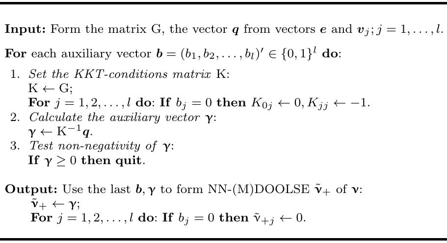
"## KKT algorithm\n",
"using the the KKT algorithm (tab.3, _Hancova et al 2019_) \n",
" \n",
"\n",
"$~$\n",
">$\n",
"\\qquad \\mathbf{q} = \n",
"\\left(\\begin{array}{c}\n",
"\\mathbf{e}' \\mathbf{e}\\\\\n",
"(\\mathbf{e}' \\mathbf{v}_{1})^2 \\\\\n",
"\\vdots \\\\\n",
"(\\mathbf{e}' \\mathbf{v}_{l})^2\n",
"\\end{array}\\right)\n",
"$\n",
">\n",
"> $\\qquad\\mathrm{G} = \\left(\\begin{array}{ccccc}\n",
"\\small\n",
"n^* & ||\\mathbf{v}_{1}||^2 & ||\\mathbf{v}_{2}||^2 & \\ldots & ||\\mathbf{v}_{l}||^2 \\\\\n",
"||\\mathbf{v}_{1}||^2 & ||\\mathbf{v}_{1}||^4 & 0 & \\ldots & 0 \\\\\n",
"||\\mathbf{v}_{2}||^2 & 0 & ||\\mathbf{v}_{2}||^4 & \\ldots & 0 \\\\\n",
"\\vdots & \\vdots & \\vdots & \\ldots & \\vdots \\\\\n",
"||\\mathbf{v}_{l}||^2 & 0 & 0 & \\ldots & ||\\mathbf{v}_{l}||^4\n",
"\\end{array}\\right)\n",
"$"
]
},
{
"cell_type": "markdown",
"metadata": {},
"source": [
"## SciPy(Numpy)"
]
},
{
"cell_type": "code",
"execution_count": 14,
"metadata": {
"ExecuteTime": {
"end_time": "2019-05-12T14:02:10.518000Z",
"start_time": "2019-05-12T14:02:10.496000Z"
}
},
"outputs": [
{
"name": "stdout",
"output_type": "stream",
"text": [
"[0.1032430972 0.0011886967 0.2275893252 0.0209146692] 0.2507885054268491 (1, 1, 1)\n"
]
}
],
"source": [
"## SciPy(Numpy)# Input: form G\n",
"ns, nvj = n, norm(V, axis=0)\n",
"u, v, Q = np.mat(ns), np.mat(nvj**2), np.diag(nvj**4)\n",
"G = np.bmat([[u,v],[v.T,Q]])\n",
"# form q\n",
"e2, Ve2 = ec*e, np.multiply(Vc*e, Vc*e)\n",
"q = np.vstack((e2, Ve2))\n",
"\n",
"# body of the algorithm\n",
"for b in product([0,1], repeat=l): \n",
" # set the KKT-conditions matrix K\n",
" K = G*1\n",
" for j in range(1,l+1): \n",
" if b[j-1] == 0: K[0,j], K[j,j] = 0,-1\n",
" # calculate the auxiliary vector g\n",
" g = inv(K)*q\n",
" # test non-negativity g\n",
" if (g >= 0).all(): break \n",
"\n",
"# Output: Form estimates nu\n",
"nu = g*1\n",
"for j in range(1,l+1):\n",
" if b[j-1] == 0: nu[j] = 0\n",
"\n",
"NN_DOOLSE = np.array(nu).flatten()\n",
"print(NN_DOOLSE, norm(NN_DOOLSE),b)"
]
},
{
"cell_type": "markdown",
"metadata": {},
"source": [
"## CVXPY\n",
"\n",
"nonnegative DOOLSE as a convex optimization problem\n",
"\n",
">$\n",
"\\begin{array}{ll} \n",
"\\textit{minimize} & f_0(\\boldsymbol{\\nu})=||\\mathbf{e}\\mathbf{e}'-\\Sigma_\\boldsymbol{\\nu}||^2 \\\\[6pt]\n",
"\\textit{subject to} & \\boldsymbol{\\nu} = \\left(\\nu_0, \\ldots, \\nu_l\\right)'\\in [0, \\infty)^{l+1} \n",
"\\end{array}\n",
"$"
]
},
{
"cell_type": "code",
"execution_count": 15,
"metadata": {
"ExecuteTime": {
"end_time": "2019-05-12T14:02:10.617000Z",
"start_time": "2019-05-12T14:02:10.525000Z"
},
"scrolled": true
},
"outputs": [
{
"name": "stdout",
"output_type": "stream",
"text": [
"NN-DOOLSEcvx = [0.103243196 0.001188791 0.2275893166 0.0209146922] norm= 0.2507885406842395\n"
]
}
],
"source": [
"# set the optimization variable, objective function\n",
"v = Variable(l+1)\n",
"fv = sum_squares(e*e.T - v[0]*In - V*diag(v[1:])*V.T)\n",
"\n",
"# construct the problem for DOOLSE\n",
"objective = Minimize(fv)\n",
"constraints = [v >= 0]\n",
"prob = Problem(objective,constraints)\n",
"\n",
"# solve the DOOLSE problem\n",
"prob.solve()\n",
"\n",
"NN_DOOLSEcvx = v.value\n",
"print('NN-DOOLSEcvx =', NN_DOOLSEcvx, 'norm=', norm(NN_DOOLSEcvx))"
]
},
{
"cell_type": "markdown",
"metadata": {},
"source": [
"## CVXPY\n",
"\n",
"using equivalent (RE)MLE convex problem (proposition 5, _Hancova et al 2019_)\n",
"\n",
"\n",
">$\n",
"\\begin{array}{ll} \n",
"\\textit{minimize} & \\quad f_0(\\mathbf{d})=-(n^*\\!-l)\\ln d_0 - \\displaystyle\\sum\\limits_{j=1}^{l} \n",
"\t\t\\ln(d_0-d_j||\\mathbf{v}_j||^2+d_0\\mathbf{e}'\\mathbf{e}-\\mathbf{e}'\\mathrm{V}\\,\\mathrm{diag}\\{d_j\\}\\mathrm{V}'\\mathbf{e} \\\\[6pt]\n",
"\\textit{subject to} & \\quad d_0 > \\max\\{d_j||\\mathbf{v}_j||^2, j = 1, \\ldots, l\\} \\\\\n",
" & \\quad d_j \\geq 0, j=1,\\ldots l \\\\\n",
" & \\\\\n",
"& \\quad\\text{for MLE: } n^* = n, \\text{ for REMLE: } n^* = n-k \\\\\n",
"\\textit{back transformation:} & \\quad \\nu_0 = \\dfrac{1}{d_0}, \\nu_j = \\dfrac{d_j}{d_0\\left(d_0 -d_j||\\mathbf{v}_j||^2\\right)}\n",
"\\end{array}\n",
"$"
]
},
{
"cell_type": "code",
"execution_count": 16,
"metadata": {
"ExecuteTime": {
"end_time": "2019-05-12T14:02:10.664000Z",
"start_time": "2019-05-12T14:02:10.623000Z"
}
},
"outputs": [
{
"name": "stdout",
"output_type": "stream",
"text": [
"REMLEcvx = [0.1032431005586019, 0.001188696520735739, 0.22758937066419727, 0.020914668029817677] norm = 0.25078854796520283\n"
]
}
],
"source": [
"# set variables for the objective\n",
"ns = n\n",
"d = Variable(l+1)\n",
"logdetS = (ns-l)*log(d[0])+sum(log(d[0]-GV*d[1:]))\n",
"\n",
"# construct the problem\n",
"objective = Maximize(logdetS-(d[0]*ec*e-ec*V*diag(d[1:])*Vc*e))\n",
"constraints = [0 <= d[1:], max(GV*d[1:]) <= d[0]]\n",
"prob = Problem(objective,constraints)\n",
"\n",
"# solve the problem\n",
"solution = prob.solve()\n",
"dv = d.value.tolist()\n",
"\n",
"# back transformation\n",
"s0 = [1/dv[0]]\n",
"sj = [dv[i]/(dv[0]*(dv[0]-dv[i]*GV[i-1,i-1])) for i in range(1,l+1)]\n",
"sv = s0+sj\n",
"\n",
"print('REMLEcvx = ', sv, ' norm = ', norm(sv))"
]
},
{
"cell_type": "markdown",
"metadata": {},
"source": [
"## $\\boldsymbol{2^{nd}}$ stage of EBLUP-NE"
]
},
{
"cell_type": "markdown",
"metadata": {},
"source": [
"## SciPy(Numpy)"
]
},
{
"cell_type": "code",
"execution_count": 17,
"metadata": {
"ExecuteTime": {
"end_time": "2019-05-12T14:02:10.676000Z",
"start_time": "2019-05-12T14:02:10.669000Z"
}
},
"outputs": [
{
"name": "stdout",
"output_type": "stream",
"text": [
"[1, 0.09263221759409881, 0.9765451623936303, 0.8817377950062207]\n"
]
}
],
"source": [
"## SciPy(Numpy)# numerical results\n",
"print(rho2(NN_DOOLSE))"
]
},
{
"cell_type": "code",
"execution_count": 18,
"metadata": {
"ExecuteTime": {
"end_time": "2019-05-12T14:02:10.688000Z",
"start_time": "2019-05-12T14:02:10.681000Z"
}
},
"outputs": [
{
"name": "stdout",
"output_type": "stream",
"text": [
"[0.10766780139512397, 0.00036178626837732086, 0.2249044531342338, 0.01963906145797461] 0.2501203552714627\n"
]
}
],
"source": [
"print(EBLUPNE(NN_DOOLSE),norm(EBLUPNE(NN_DOOLSE)))"
]
},
{
"cell_type": "code",
"execution_count": 19,
"metadata": {
"ExecuteTime": {
"end_time": "2019-05-12T14:02:10.702000Z",
"start_time": "2019-05-12T14:02:10.694000Z"
},
"scrolled": true
},
"outputs": [
{
"name": "stdout",
"output_type": "stream",
"text": [
"[0.10766780139512397, 0.0003617862683773213, 0.2249044531342336, 0.01963906145797493] 0.25012035527146254\n"
]
}
],
"source": [
"#cross-checking\n",
"print(EBLUPNEgen(NN_DOOLSE), norm(EBLUPNEgen(NN_DOOLSE)))"
]
},
{
"cell_type": "markdown",
"metadata": {},
"source": [
"***\n",
"\n",
"# NN-MDOOLSE or REMLE\n",
"\n",
"## $\\boldsymbol{1^{st}}$ stage of EBLUP-NE "
]
},
{
"cell_type": "markdown",
"metadata": {},
"source": [
"## KKT algorithm"
]
},
{
"cell_type": "markdown",
"metadata": {},
"source": [
"## SciPy(Numpy)"
]
},
{
"cell_type": "code",
"execution_count": 20,
"metadata": {
"ExecuteTime": {
"end_time": "2019-05-12T14:02:10.729000Z",
"start_time": "2019-05-12T14:02:10.707000Z"
}
},
"outputs": [
{
"name": "stdout",
"output_type": "stream",
"text": [
"[0.1076678014 0.0010722571 0.2274728856 0.0208564495] 0.2525319986886 (1, 1, 1)\n"
]
}
],
"source": [
"# Input: form G\n",
"ns, nvj = n-k, norm(V, axis=0)\n",
"u, v, Q = np.mat(ns), np.mat(nvj**2), np.diag(nvj**4)\n",
"G = np.bmat([[u,v],[v.T,Q]])\n",
"# form q\n",
"e2, Ve2 = ec*e, np.multiply(Vc*e, Vc*e)\n",
"q = np.vstack((e2, Ve2))\n",
"\n",
"# body of the algorithm\n",
"for b in product([0,1], repeat=l): \n",
" # set the KKT-conditions matrix K\n",
" K = G*1\n",
" for j in range(1,l+1): \n",
" if b[j-1] == 0: K[0,j], K[j,j] = 0,-1\n",
" # calculate the auxiliary vector g\n",
" g = inv(K)*q\n",
" # test non-negativity g\n",
" if (g >= 0).all(): break \n",
"\n",
"# Output: Form estimates nu\n",
"nu = g*1\n",
"for j in range(1,l+1):\n",
" if b[j-1] == 0: nu[j] = 0\n",
"\n",
"NN_MDOOLSE = np.array(nu).flatten()\n",
"print(NN_MDOOLSE, norm(NN_MDOOLSE),b)"
]
},
{
"cell_type": "markdown",
"metadata": {},
"source": [
"## CVXPY\n",
"\n",
"nonnegative DOOLSE as a convex optimization problem\n",
"\n",
">$\n",
"\\begin{array}{ll} \n",
"\\textit{minimize} & f_0(\\boldsymbol{\\nu})=||\\mathbf{e}\\mathbf{e}'-\\mathrm{M_F}\\Sigma_\\boldsymbol{\\nu}\\mathrm{M_F}||^2 \\\\[6pt]\n",
"\\textit{subject to} & \\boldsymbol{\\nu} = \\left(\\nu_0, \\ldots, \\nu_l\\right)'\\in [0, \\infty)^{l+1} \n",
"\\end{array}\n",
"$"
]
},
{
"cell_type": "code",
"execution_count": 21,
"metadata": {
"ExecuteTime": {
"end_time": "2019-05-12T14:02:10.839000Z",
"start_time": "2019-05-12T14:02:10.736000Z"
}
},
"outputs": [
{
"name": "stdout",
"output_type": "stream",
"text": [
"NN-MDOOLSEcvx = [0.107668313 0.0010725165 0.2274728524 0.020856525 ] norm = 0.2525321942497591\n"
]
}
],
"source": [
"# set the optimization variable, objective function\n",
"v = Variable(l+1)\n",
"fv = sum_squares(e*ec - v[0]*MF - V*diag(v[1:])*Vc)\n",
"\n",
"# the optimization problem for MDOOLSE\n",
"objective = Minimize(fv)\n",
"constraints = [v >= 0]\n",
"prob = Problem(objective,constraints)\n",
"\n",
"# solve the MDOOLSE problem\n",
"prob.solve()\n",
"NN_MDOOLSEcvx = v.value\n",
"print('NN-MDOOLSEcvx =', NN_MDOOLSEcvx, 'norm =', norm(NN_MDOOLSEcvx) )"
]
},
{
"cell_type": "markdown",
"metadata": {},
"source": [
"## CVXPY\n",
"\n",
"using equivalent (RE)MLE convex problem (proposition 5, _Hancova et al 2019_)\n",
"\n",
"\n",
">$\n",
"\\begin{array}{ll} \n",
"\\textit{minimize} & \\quad f_0(\\mathbf{d})=-(n^*\\!-l)\\ln d_0 - \\displaystyle\\sum\\limits_{j=1}^{l} \n",
"\t\t\\ln(d_0-d_j||\\mathbf{v}_j||^2+d_0\\mathbf{e}'\\mathbf{e}-\\mathbf{e}'\\mathrm{V}\\,\\mathrm{diag}\\{d_j\\}\\mathrm{V}'\\mathbf{e} \\\\[6pt]\n",
"\\textit{subject to} & \\quad d_0 > \\max\\{d_j||\\mathbf{v}_j||^2, j = 1, \\ldots, l\\} \\\\\n",
" & \\quad d_j \\geq 0, j=1,\\ldots l \\\\\n",
" & \\\\\n",
"& \\quad\\text{for MLE: } n^* = n, \\text{ for REMLE: } n^* = n-k \\\\\n",
"\\textit{back transformation:} & \\quad \\nu_0 = \\dfrac{1}{d_0}, \\nu_j = \\dfrac{d_j}{d_0\\left(d_0 -d_j||\\mathbf{v}_j||^2\\right)}\n",
"\\end{array}\n",
"$"
]
},
{
"cell_type": "code",
"execution_count": 22,
"metadata": {
"ExecuteTime": {
"end_time": "2019-05-12T14:02:10.885000Z",
"start_time": "2019-05-12T14:02:10.844000Z"
}
},
"outputs": [
{
"name": "stdout",
"output_type": "stream",
"text": [
"REMLEcvx = [0.10766780248874558, 0.001072255859342178, 0.22747309845443972, 0.020856451321299943] norm = 0.25253219103228086\n"
]
}
],
"source": [
"# set variables for the objective\n",
"ns = n - k\n",
"d = Variable(l+1)\n",
"logdetS = (ns-l)*log(d[0])+sum(log(d[0]-GV*d[1:]))\n",
"\n",
"# construct the problem\n",
"objective = Maximize(logdetS-(d[0]*ec*e-ec*V*diag(d[1:])*Vc*e))\n",
"constraints = [0 <= d[1:], max(GV*d[1:]) <= d[0]]\n",
"prob = Problem(objective,constraints)\n",
"\n",
"# solve the problem\n",
"solution = prob.solve()\n",
"dv = d.value.tolist()\n",
"\n",
"# back transformation\n",
"s0 = [1/dv[0]]\n",
"sj = [dv[i]/(dv[0]*(dv[0]-dv[i]*GV[i-1,i-1])) for i in range(1,l+1)]\n",
"sv = s0+sj\n",
"\n",
"print('REMLEcvx = ', sv, ' norm = ', norm(sv))"
]
},
{
"cell_type": "markdown",
"metadata": {},
"source": [
"## $\\boldsymbol{2^{nd}}$ stage of EBLUP-NE"
]
},
{
"cell_type": "markdown",
"metadata": {},
"source": [
"## SciPy(Numpy)"
]
},
{
"cell_type": "code",
"execution_count": 23,
"metadata": {
"ExecuteTime": {
"end_time": "2019-05-12T14:02:10.898000Z",
"start_time": "2019-05-12T14:02:10.890000Z"
}
},
"outputs": [
{
"name": "stdout",
"output_type": "stream",
"text": [
"[1, 0.07537335031457347, 0.9755461750828655, 0.8768356719511479]\n"
]
}
],
"source": [
"## SciPy(Numpy)# numerical results\n",
"print(rho2(NN_MDOOLSE))"
]
},
{
"cell_type": "code",
"execution_count": 24,
"metadata": {
"ExecuteTime": {
"end_time": "2019-05-12T14:02:10.914000Z",
"start_time": "2019-05-12T14:02:10.904000Z"
}
},
"outputs": [
{
"name": "stdout",
"output_type": "stream",
"text": [
"[0.10766780139512397, 0.00029437968617889685, 0.22467438011409316, 0.01952987582875651] 0.2499048523862595\n"
]
}
],
"source": [
"print(EBLUPNE(NN_MDOOLSE),norm(EBLUPNE(NN_MDOOLSE)))"
]
},
{
"cell_type": "code",
"execution_count": 25,
"metadata": {
"ExecuteTime": {
"end_time": "2019-05-12T14:02:10.928000Z",
"start_time": "2019-05-12T14:02:10.919000Z"
},
"scrolled": false
},
"outputs": [
{
"name": "stdout",
"output_type": "stream",
"text": [
"[0.10766780139512397, 0.00029437968617889316, 0.22467438011409285, 0.019529875828756697] 0.24990485238625926\n"
]
}
],
"source": [
"#cross-checking\n",
"print(EBLUPNEgen(NN_MDOOLSE), norm(EBLUPNEgen(NN_MDOOLSE)))"
]
},
{
"cell_type": "markdown",
"metadata": {},
"source": [
"***\n",
"\n",
"# References \n",
"This notebook belongs to suplementary materials of the paper submitted to Statistical Papers and available at .\n",
"\n",
"* Hančová, M., Vozáriková, G., Gajdoš, A., Hanč, J. (2019). [Estimating variance components in time series\n",
"\tlinear regression models using empirical BLUPs and convex optimization](https://arxiv.org/abs/1905.07771), https://arxiv.org/, 2019. \n",
"\n",
"### Abstract of the paper\n",
"\n",
"We propose a two-stage estimation method of variance components in time series models known as FDSLRMs, whose observations can be described by a linear mixed model (LMM). We based estimating variances, fundamental quantities in a time series forecasting approach called kriging, on the empirical (plug-in) best linear unbiased predictions of unobservable random components in FDSLRM. \n",
"\n",
"The method, providing invariant non-negative quadratic estimators, can be used for any absolutely continuous probability distribution of time series data. As a result of applying the convex optimization and the LMM methodology, we resolved two problems $-$ theoretical existence and equivalence between least squares estimators, non-negative (M)DOOLSE, and maximum likelihood estimators, (RE)MLE, as possible starting points of our method and a \n",
"practical lack of computational implementation for FDSLRM. As for computing (RE)MLE in the case of $ n $ observed time series values, we also discovered a new algorithm of order $\\mathcal{O}(n)$, which at the default precision is $10^7$ times more accurate and $n^2$ times faster than the best current Python(or R)-based computational packages, namely CVXPY, CVXR, nlme, sommer and mixed. \n",
"\n",
"We illustrate our results on three real data sets $-$ electricity consumption, tourism and cyber security $-$ which are easily available, reproducible, sharable and modifiable in the form of interactive Jupyter notebooks."
]
},
{
"cell_type": "markdown",
"metadata": {},
"source": [
"* Hyndman R.J., Athanasopoulos G. (2018). [Forecasting: Principles and Practice](https://otexts.org/fpp2/) (2nd Edition), OTexts, Monash University, Australia. Data in R package fpp2 version 2.3. https://CRAN.R-project.org/package=fpp2"
]
},
{
"cell_type": "markdown",
"metadata": {},
"source": [
"| [Table of Contents](#table_of_contents) | [Data and model](#data_and_model) | [Natural estimators](#natural_estimators) | [NN-DOOLSE, MLE](#doolse) | [NN-MDOOLSE, REMLE](#mdoolse) | [References](#references) |"
]
}
],
"metadata": {
"kernelspec": {
"display_name": "Python 2.7",
"language": "python",
"name": "python2"
},
"language_info": {
"codemirror_mode": {
"name": "ipython",
"version": 2
},
"file_extension": ".py",
"mimetype": "text/x-python",
"name": "python",
"nbconvert_exporter": "python",
"pygments_lexer": "ipython2",
"version": "2.7.16"
},
"varInspector": {
"cols": {
"lenName": 16,
"lenType": 16,
"lenVar": 40
},
"kernels_config": {
"python": {
"delete_cmd_postfix": "",
"delete_cmd_prefix": "del ",
"library": "var_list.py",
"varRefreshCmd": "print(var_dic_list())"
},
"r": {
"delete_cmd_postfix": ") ",
"delete_cmd_prefix": "rm(",
"library": "var_list.r",
"varRefreshCmd": "cat(var_dic_list()) "
}
},
"types_to_exclude": [
"module",
"function",
"builtin_function_or_method",
"instance",
"_Feature"
],
"window_display": false
}
},
"nbformat": 4,
"nbformat_minor": 2
}
\n",
"\n",
"$~$\n",
">$\n",
"\\qquad \\mathbf{q} = \n",
"\\left(\\begin{array}{c}\n",
"\\mathbf{e}' \\mathbf{e}\\\\\n",
"(\\mathbf{e}' \\mathbf{v}_{1})^2 \\\\\n",
"\\vdots \\\\\n",
"(\\mathbf{e}' \\mathbf{v}_{l})^2\n",
"\\end{array}\\right)\n",
"$\n",
">\n",
"> $\\qquad\\mathrm{G} = \\left(\\begin{array}{ccccc}\n",
"\\small\n",
"n^* & ||\\mathbf{v}_{1}||^2 & ||\\mathbf{v}_{2}||^2 & \\ldots & ||\\mathbf{v}_{l}||^2 \\\\\n",
"||\\mathbf{v}_{1}||^2 & ||\\mathbf{v}_{1}||^4 & 0 & \\ldots & 0 \\\\\n",
"||\\mathbf{v}_{2}||^2 & 0 & ||\\mathbf{v}_{2}||^4 & \\ldots & 0 \\\\\n",
"\\vdots & \\vdots & \\vdots & \\ldots & \\vdots \\\\\n",
"||\\mathbf{v}_{l}||^2 & 0 & 0 & \\ldots & ||\\mathbf{v}_{l}||^4\n",
"\\end{array}\\right)\n",
"$"
]
},
{
"cell_type": "markdown",
"metadata": {},
"source": [
"## SciPy(Numpy)"
]
},
{
"cell_type": "code",
"execution_count": 14,
"metadata": {
"ExecuteTime": {
"end_time": "2019-05-12T14:02:10.518000Z",
"start_time": "2019-05-12T14:02:10.496000Z"
}
},
"outputs": [
{
"name": "stdout",
"output_type": "stream",
"text": [
"[0.1032430972 0.0011886967 0.2275893252 0.0209146692] 0.2507885054268491 (1, 1, 1)\n"
]
}
],
"source": [
"## SciPy(Numpy)# Input: form G\n",
"ns, nvj = n, norm(V, axis=0)\n",
"u, v, Q = np.mat(ns), np.mat(nvj**2), np.diag(nvj**4)\n",
"G = np.bmat([[u,v],[v.T,Q]])\n",
"# form q\n",
"e2, Ve2 = ec*e, np.multiply(Vc*e, Vc*e)\n",
"q = np.vstack((e2, Ve2))\n",
"\n",
"# body of the algorithm\n",
"for b in product([0,1], repeat=l): \n",
" # set the KKT-conditions matrix K\n",
" K = G*1\n",
" for j in range(1,l+1): \n",
" if b[j-1] == 0: K[0,j], K[j,j] = 0,-1\n",
" # calculate the auxiliary vector g\n",
" g = inv(K)*q\n",
" # test non-negativity g\n",
" if (g >= 0).all(): break \n",
"\n",
"# Output: Form estimates nu\n",
"nu = g*1\n",
"for j in range(1,l+1):\n",
" if b[j-1] == 0: nu[j] = 0\n",
"\n",
"NN_DOOLSE = np.array(nu).flatten()\n",
"print(NN_DOOLSE, norm(NN_DOOLSE),b)"
]
},
{
"cell_type": "markdown",
"metadata": {},
"source": [
"## CVXPY\n",
"\n",
"nonnegative DOOLSE as a convex optimization problem\n",
"\n",
">$\n",
"\\begin{array}{ll} \n",
"\\textit{minimize} & f_0(\\boldsymbol{\\nu})=||\\mathbf{e}\\mathbf{e}'-\\Sigma_\\boldsymbol{\\nu}||^2 \\\\[6pt]\n",
"\\textit{subject to} & \\boldsymbol{\\nu} = \\left(\\nu_0, \\ldots, \\nu_l\\right)'\\in [0, \\infty)^{l+1} \n",
"\\end{array}\n",
"$"
]
},
{
"cell_type": "code",
"execution_count": 15,
"metadata": {
"ExecuteTime": {
"end_time": "2019-05-12T14:02:10.617000Z",
"start_time": "2019-05-12T14:02:10.525000Z"
},
"scrolled": true
},
"outputs": [
{
"name": "stdout",
"output_type": "stream",
"text": [
"NN-DOOLSEcvx = [0.103243196 0.001188791 0.2275893166 0.0209146922] norm= 0.2507885406842395\n"
]
}
],
"source": [
"# set the optimization variable, objective function\n",
"v = Variable(l+1)\n",
"fv = sum_squares(e*e.T - v[0]*In - V*diag(v[1:])*V.T)\n",
"\n",
"# construct the problem for DOOLSE\n",
"objective = Minimize(fv)\n",
"constraints = [v >= 0]\n",
"prob = Problem(objective,constraints)\n",
"\n",
"# solve the DOOLSE problem\n",
"prob.solve()\n",
"\n",
"NN_DOOLSEcvx = v.value\n",
"print('NN-DOOLSEcvx =', NN_DOOLSEcvx, 'norm=', norm(NN_DOOLSEcvx))"
]
},
{
"cell_type": "markdown",
"metadata": {},
"source": [
"## CVXPY\n",
"\n",
"using equivalent (RE)MLE convex problem (proposition 5, _Hancova et al 2019_)\n",
"\n",
"\n",
">$\n",
"\\begin{array}{ll} \n",
"\\textit{minimize} & \\quad f_0(\\mathbf{d})=-(n^*\\!-l)\\ln d_0 - \\displaystyle\\sum\\limits_{j=1}^{l} \n",
"\t\t\\ln(d_0-d_j||\\mathbf{v}_j||^2+d_0\\mathbf{e}'\\mathbf{e}-\\mathbf{e}'\\mathrm{V}\\,\\mathrm{diag}\\{d_j\\}\\mathrm{V}'\\mathbf{e} \\\\[6pt]\n",
"\\textit{subject to} & \\quad d_0 > \\max\\{d_j||\\mathbf{v}_j||^2, j = 1, \\ldots, l\\} \\\\\n",
" & \\quad d_j \\geq 0, j=1,\\ldots l \\\\\n",
" & \\\\\n",
"& \\quad\\text{for MLE: } n^* = n, \\text{ for REMLE: } n^* = n-k \\\\\n",
"\\textit{back transformation:} & \\quad \\nu_0 = \\dfrac{1}{d_0}, \\nu_j = \\dfrac{d_j}{d_0\\left(d_0 -d_j||\\mathbf{v}_j||^2\\right)}\n",
"\\end{array}\n",
"$"
]
},
{
"cell_type": "code",
"execution_count": 16,
"metadata": {
"ExecuteTime": {
"end_time": "2019-05-12T14:02:10.664000Z",
"start_time": "2019-05-12T14:02:10.623000Z"
}
},
"outputs": [
{
"name": "stdout",
"output_type": "stream",
"text": [
"REMLEcvx = [0.1032431005586019, 0.001188696520735739, 0.22758937066419727, 0.020914668029817677] norm = 0.25078854796520283\n"
]
}
],
"source": [
"# set variables for the objective\n",
"ns = n\n",
"d = Variable(l+1)\n",
"logdetS = (ns-l)*log(d[0])+sum(log(d[0]-GV*d[1:]))\n",
"\n",
"# construct the problem\n",
"objective = Maximize(logdetS-(d[0]*ec*e-ec*V*diag(d[1:])*Vc*e))\n",
"constraints = [0 <= d[1:], max(GV*d[1:]) <= d[0]]\n",
"prob = Problem(objective,constraints)\n",
"\n",
"# solve the problem\n",
"solution = prob.solve()\n",
"dv = d.value.tolist()\n",
"\n",
"# back transformation\n",
"s0 = [1/dv[0]]\n",
"sj = [dv[i]/(dv[0]*(dv[0]-dv[i]*GV[i-1,i-1])) for i in range(1,l+1)]\n",
"sv = s0+sj\n",
"\n",
"print('REMLEcvx = ', sv, ' norm = ', norm(sv))"
]
},
{
"cell_type": "markdown",
"metadata": {},
"source": [
"## $\\boldsymbol{2^{nd}}$ stage of EBLUP-NE"
]
},
{
"cell_type": "markdown",
"metadata": {},
"source": [
"## SciPy(Numpy)"
]
},
{
"cell_type": "code",
"execution_count": 17,
"metadata": {
"ExecuteTime": {
"end_time": "2019-05-12T14:02:10.676000Z",
"start_time": "2019-05-12T14:02:10.669000Z"
}
},
"outputs": [
{
"name": "stdout",
"output_type": "stream",
"text": [
"[1, 0.09263221759409881, 0.9765451623936303, 0.8817377950062207]\n"
]
}
],
"source": [
"## SciPy(Numpy)# numerical results\n",
"print(rho2(NN_DOOLSE))"
]
},
{
"cell_type": "code",
"execution_count": 18,
"metadata": {
"ExecuteTime": {
"end_time": "2019-05-12T14:02:10.688000Z",
"start_time": "2019-05-12T14:02:10.681000Z"
}
},
"outputs": [
{
"name": "stdout",
"output_type": "stream",
"text": [
"[0.10766780139512397, 0.00036178626837732086, 0.2249044531342338, 0.01963906145797461] 0.2501203552714627\n"
]
}
],
"source": [
"print(EBLUPNE(NN_DOOLSE),norm(EBLUPNE(NN_DOOLSE)))"
]
},
{
"cell_type": "code",
"execution_count": 19,
"metadata": {
"ExecuteTime": {
"end_time": "2019-05-12T14:02:10.702000Z",
"start_time": "2019-05-12T14:02:10.694000Z"
},
"scrolled": true
},
"outputs": [
{
"name": "stdout",
"output_type": "stream",
"text": [
"[0.10766780139512397, 0.0003617862683773213, 0.2249044531342336, 0.01963906145797493] 0.25012035527146254\n"
]
}
],
"source": [
"#cross-checking\n",
"print(EBLUPNEgen(NN_DOOLSE), norm(EBLUPNEgen(NN_DOOLSE)))"
]
},
{
"cell_type": "markdown",
"metadata": {},
"source": [
"***\n",
"\n",
"# NN-MDOOLSE or REMLE\n",
"\n",
"## $\\boldsymbol{1^{st}}$ stage of EBLUP-NE "
]
},
{
"cell_type": "markdown",
"metadata": {},
"source": [
"## KKT algorithm"
]
},
{
"cell_type": "markdown",
"metadata": {},
"source": [
"## SciPy(Numpy)"
]
},
{
"cell_type": "code",
"execution_count": 20,
"metadata": {
"ExecuteTime": {
"end_time": "2019-05-12T14:02:10.729000Z",
"start_time": "2019-05-12T14:02:10.707000Z"
}
},
"outputs": [
{
"name": "stdout",
"output_type": "stream",
"text": [
"[0.1076678014 0.0010722571 0.2274728856 0.0208564495] 0.2525319986886 (1, 1, 1)\n"
]
}
],
"source": [
"# Input: form G\n",
"ns, nvj = n-k, norm(V, axis=0)\n",
"u, v, Q = np.mat(ns), np.mat(nvj**2), np.diag(nvj**4)\n",
"G = np.bmat([[u,v],[v.T,Q]])\n",
"# form q\n",
"e2, Ve2 = ec*e, np.multiply(Vc*e, Vc*e)\n",
"q = np.vstack((e2, Ve2))\n",
"\n",
"# body of the algorithm\n",
"for b in product([0,1], repeat=l): \n",
" # set the KKT-conditions matrix K\n",
" K = G*1\n",
" for j in range(1,l+1): \n",
" if b[j-1] == 0: K[0,j], K[j,j] = 0,-1\n",
" # calculate the auxiliary vector g\n",
" g = inv(K)*q\n",
" # test non-negativity g\n",
" if (g >= 0).all(): break \n",
"\n",
"# Output: Form estimates nu\n",
"nu = g*1\n",
"for j in range(1,l+1):\n",
" if b[j-1] == 0: nu[j] = 0\n",
"\n",
"NN_MDOOLSE = np.array(nu).flatten()\n",
"print(NN_MDOOLSE, norm(NN_MDOOLSE),b)"
]
},
{
"cell_type": "markdown",
"metadata": {},
"source": [
"## CVXPY\n",
"\n",
"nonnegative DOOLSE as a convex optimization problem\n",
"\n",
">$\n",
"\\begin{array}{ll} \n",
"\\textit{minimize} & f_0(\\boldsymbol{\\nu})=||\\mathbf{e}\\mathbf{e}'-\\mathrm{M_F}\\Sigma_\\boldsymbol{\\nu}\\mathrm{M_F}||^2 \\\\[6pt]\n",
"\\textit{subject to} & \\boldsymbol{\\nu} = \\left(\\nu_0, \\ldots, \\nu_l\\right)'\\in [0, \\infty)^{l+1} \n",
"\\end{array}\n",
"$"
]
},
{
"cell_type": "code",
"execution_count": 21,
"metadata": {
"ExecuteTime": {
"end_time": "2019-05-12T14:02:10.839000Z",
"start_time": "2019-05-12T14:02:10.736000Z"
}
},
"outputs": [
{
"name": "stdout",
"output_type": "stream",
"text": [
"NN-MDOOLSEcvx = [0.107668313 0.0010725165 0.2274728524 0.020856525 ] norm = 0.2525321942497591\n"
]
}
],
"source": [
"# set the optimization variable, objective function\n",
"v = Variable(l+1)\n",
"fv = sum_squares(e*ec - v[0]*MF - V*diag(v[1:])*Vc)\n",
"\n",
"# the optimization problem for MDOOLSE\n",
"objective = Minimize(fv)\n",
"constraints = [v >= 0]\n",
"prob = Problem(objective,constraints)\n",
"\n",
"# solve the MDOOLSE problem\n",
"prob.solve()\n",
"NN_MDOOLSEcvx = v.value\n",
"print('NN-MDOOLSEcvx =', NN_MDOOLSEcvx, 'norm =', norm(NN_MDOOLSEcvx) )"
]
},
{
"cell_type": "markdown",
"metadata": {},
"source": [
"## CVXPY\n",
"\n",
"using equivalent (RE)MLE convex problem (proposition 5, _Hancova et al 2019_)\n",
"\n",
"\n",
">$\n",
"\\begin{array}{ll} \n",
"\\textit{minimize} & \\quad f_0(\\mathbf{d})=-(n^*\\!-l)\\ln d_0 - \\displaystyle\\sum\\limits_{j=1}^{l} \n",
"\t\t\\ln(d_0-d_j||\\mathbf{v}_j||^2+d_0\\mathbf{e}'\\mathbf{e}-\\mathbf{e}'\\mathrm{V}\\,\\mathrm{diag}\\{d_j\\}\\mathrm{V}'\\mathbf{e} \\\\[6pt]\n",
"\\textit{subject to} & \\quad d_0 > \\max\\{d_j||\\mathbf{v}_j||^2, j = 1, \\ldots, l\\} \\\\\n",
" & \\quad d_j \\geq 0, j=1,\\ldots l \\\\\n",
" & \\\\\n",
"& \\quad\\text{for MLE: } n^* = n, \\text{ for REMLE: } n^* = n-k \\\\\n",
"\\textit{back transformation:} & \\quad \\nu_0 = \\dfrac{1}{d_0}, \\nu_j = \\dfrac{d_j}{d_0\\left(d_0 -d_j||\\mathbf{v}_j||^2\\right)}\n",
"\\end{array}\n",
"$"
]
},
{
"cell_type": "code",
"execution_count": 22,
"metadata": {
"ExecuteTime": {
"end_time": "2019-05-12T14:02:10.885000Z",
"start_time": "2019-05-12T14:02:10.844000Z"
}
},
"outputs": [
{
"name": "stdout",
"output_type": "stream",
"text": [
"REMLEcvx = [0.10766780248874558, 0.001072255859342178, 0.22747309845443972, 0.020856451321299943] norm = 0.25253219103228086\n"
]
}
],
"source": [
"# set variables for the objective\n",
"ns = n - k\n",
"d = Variable(l+1)\n",
"logdetS = (ns-l)*log(d[0])+sum(log(d[0]-GV*d[1:]))\n",
"\n",
"# construct the problem\n",
"objective = Maximize(logdetS-(d[0]*ec*e-ec*V*diag(d[1:])*Vc*e))\n",
"constraints = [0 <= d[1:], max(GV*d[1:]) <= d[0]]\n",
"prob = Problem(objective,constraints)\n",
"\n",
"# solve the problem\n",
"solution = prob.solve()\n",
"dv = d.value.tolist()\n",
"\n",
"# back transformation\n",
"s0 = [1/dv[0]]\n",
"sj = [dv[i]/(dv[0]*(dv[0]-dv[i]*GV[i-1,i-1])) for i in range(1,l+1)]\n",
"sv = s0+sj\n",
"\n",
"print('REMLEcvx = ', sv, ' norm = ', norm(sv))"
]
},
{
"cell_type": "markdown",
"metadata": {},
"source": [
"## $\\boldsymbol{2^{nd}}$ stage of EBLUP-NE"
]
},
{
"cell_type": "markdown",
"metadata": {},
"source": [
"## SciPy(Numpy)"
]
},
{
"cell_type": "code",
"execution_count": 23,
"metadata": {
"ExecuteTime": {
"end_time": "2019-05-12T14:02:10.898000Z",
"start_time": "2019-05-12T14:02:10.890000Z"
}
},
"outputs": [
{
"name": "stdout",
"output_type": "stream",
"text": [
"[1, 0.07537335031457347, 0.9755461750828655, 0.8768356719511479]\n"
]
}
],
"source": [
"## SciPy(Numpy)# numerical results\n",
"print(rho2(NN_MDOOLSE))"
]
},
{
"cell_type": "code",
"execution_count": 24,
"metadata": {
"ExecuteTime": {
"end_time": "2019-05-12T14:02:10.914000Z",
"start_time": "2019-05-12T14:02:10.904000Z"
}
},
"outputs": [
{
"name": "stdout",
"output_type": "stream",
"text": [
"[0.10766780139512397, 0.00029437968617889685, 0.22467438011409316, 0.01952987582875651] 0.2499048523862595\n"
]
}
],
"source": [
"print(EBLUPNE(NN_MDOOLSE),norm(EBLUPNE(NN_MDOOLSE)))"
]
},
{
"cell_type": "code",
"execution_count": 25,
"metadata": {
"ExecuteTime": {
"end_time": "2019-05-12T14:02:10.928000Z",
"start_time": "2019-05-12T14:02:10.919000Z"
},
"scrolled": false
},
"outputs": [
{
"name": "stdout",
"output_type": "stream",
"text": [
"[0.10766780139512397, 0.00029437968617889316, 0.22467438011409285, 0.019529875828756697] 0.24990485238625926\n"
]
}
],
"source": [
"#cross-checking\n",
"print(EBLUPNEgen(NN_MDOOLSE), norm(EBLUPNEgen(NN_MDOOLSE)))"
]
},
{
"cell_type": "markdown",
"metadata": {},
"source": [
"***\n",
"\n",
"# References \n",
"This notebook belongs to suplementary materials of the paper submitted to Statistical Papers and available at .\n",
"\n",
"* Hančová, M., Vozáriková, G., Gajdoš, A., Hanč, J. (2019). [Estimating variance components in time series\n",
"\tlinear regression models using empirical BLUPs and convex optimization](https://arxiv.org/abs/1905.07771), https://arxiv.org/, 2019. \n",
"\n",
"### Abstract of the paper\n",
"\n",
"We propose a two-stage estimation method of variance components in time series models known as FDSLRMs, whose observations can be described by a linear mixed model (LMM). We based estimating variances, fundamental quantities in a time series forecasting approach called kriging, on the empirical (plug-in) best linear unbiased predictions of unobservable random components in FDSLRM. \n",
"\n",
"The method, providing invariant non-negative quadratic estimators, can be used for any absolutely continuous probability distribution of time series data. As a result of applying the convex optimization and the LMM methodology, we resolved two problems $-$ theoretical existence and equivalence between least squares estimators, non-negative (M)DOOLSE, and maximum likelihood estimators, (RE)MLE, as possible starting points of our method and a \n",
"practical lack of computational implementation for FDSLRM. As for computing (RE)MLE in the case of $ n $ observed time series values, we also discovered a new algorithm of order $\\mathcal{O}(n)$, which at the default precision is $10^7$ times more accurate and $n^2$ times faster than the best current Python(or R)-based computational packages, namely CVXPY, CVXR, nlme, sommer and mixed. \n",
"\n",
"We illustrate our results on three real data sets $-$ electricity consumption, tourism and cyber security $-$ which are easily available, reproducible, sharable and modifiable in the form of interactive Jupyter notebooks."
]
},
{
"cell_type": "markdown",
"metadata": {},
"source": [
"* Hyndman R.J., Athanasopoulos G. (2018). [Forecasting: Principles and Practice](https://otexts.org/fpp2/) (2nd Edition), OTexts, Monash University, Australia. Data in R package fpp2 version 2.3. https://CRAN.R-project.org/package=fpp2"
]
},
{
"cell_type": "markdown",
"metadata": {},
"source": [
"| [Table of Contents](#table_of_contents) | [Data and model](#data_and_model) | [Natural estimators](#natural_estimators) | [NN-DOOLSE, MLE](#doolse) | [NN-MDOOLSE, REMLE](#mdoolse) | [References](#references) |"
]
}
],
"metadata": {
"kernelspec": {
"display_name": "Python 2.7",
"language": "python",
"name": "python2"
},
"language_info": {
"codemirror_mode": {
"name": "ipython",
"version": 2
},
"file_extension": ".py",
"mimetype": "text/x-python",
"name": "python",
"nbconvert_exporter": "python",
"pygments_lexer": "ipython2",
"version": "2.7.16"
},
"varInspector": {
"cols": {
"lenName": 16,
"lenType": 16,
"lenVar": 40
},
"kernels_config": {
"python": {
"delete_cmd_postfix": "",
"delete_cmd_prefix": "del ",
"library": "var_list.py",
"varRefreshCmd": "print(var_dic_list())"
},
"r": {
"delete_cmd_postfix": ") ",
"delete_cmd_prefix": "rm(",
"library": "var_list.r",
"varRefreshCmd": "cat(var_dic_list()) "
}
},
"types_to_exclude": [
"module",
"function",
"builtin_function_or_method",
"instance",
"_Feature"
],
"window_display": false
}
},
"nbformat": 4,
"nbformat_minor": 2
}