{
"cells": [
{
"cell_type": "markdown",
"metadata": {},
"source": [
"| [Table of Contents](#table_of_contents) | [Data and model](#data_and_model) | [Natural estimators](#natural_estimators) | [NN-DOOLSE, MLE](#doolse) | [NN-MDOOLSE, REMLE](#mdoolse) | [References](#references) |"
]
},
{
"cell_type": "markdown",
"metadata": {},
"source": [
"**Authors:** Andrej Gajdoš, Jozef Hanč, Martina Hančová
*[Faculty of Science](https://www.upjs.sk/en/faculty-of-science/?prefferedLang=EN), P. J. Šafárik University in Košice, Slovakia*
email: [andrej.gajdos@student.upjs.sk](mailto:andrej.gajdos@student.upjs.sk)\n",
"***\n",
"** EBLUP-NE for cyber attacks** "
]
},
{
"cell_type": "markdown",
"metadata": {},
"source": [
" R-based computational tools - ** CVXR**\n",
"\n",
"### Table of Contents \n",
"* [Data and model](#data_and_model) - data and model description of empirical data\n",
"* [Natural estimators](#natural_estimators) - EBLUPNE based on NE\n",
"* [NN-DOOLSE, MLE](#doolse) - EBLUPNE based on nonnegative DOOLSE (same as MLE)\n",
"* [NN-MDOOLSE, REMLE](#mdoolse) - EBLUPNE based on nonnegative MDOOLSE (same as REMLE)\n",
"* [References](#references)\n",
"\n",
"**To get back to the contents, use the Home key.**"
]
},
{
"cell_type": "markdown",
"metadata": {},
"source": [
"## R packages"
]
},
{
"cell_type": "markdown",
"metadata": {},
"source": [
"## CVXR: R-Embedded Object-Oriented Modeling Language for Convex Optimization \n",
"\n",
"* _Purpose_: R package for solving convex optimization tasks\n",
"* _Version_: 0.99-5, 2019\n",
"* _URL_: https://cvxr.rbind.io/\n",
"* _Computational parameters_ of CVXR:\n",
"> * *solver* - the convex optimization solver ECOS, OSQP, and SCS chosen according to the given problem\n",
" * **OSQP** for convex quadratic problems\n",
" * `max_iter` - maximum number of iterations (default: 4000).\n",
" * `eps_abs` - absolute accuracy (default: 1e-3).\n",
" * `eps_rel` - relative accuracy (default: 1e-4).\n",
" * **ECOS** for convex second-order cone problems \n",
" * `maxit` - maximum number of iterations (default: 100).\n",
" * `abstol` - absolute accuracy (default: 1e-8).\n",
" * `reltol` - relative accuracy (default: 1e-8).\n",
" * `feastol` - tolerance for feasibility conditions (default: 1e-8).\n",
" * `abstol_inacc` - absolute accuracy for inaccurate solution (default: 5e-5).\n",
" * `reltol_inacc` - relative accuracy for inaccurate solution (default: 5e-5).\n",
" * `feastol_inacc` - tolerance for feasibility condition for inaccurate solution (default: 1e-4).\n",
" * **SCS** for large-scale convex cone problems\n",
" * `max_iters` - maximum number of iterations (default: 5000).\n",
" * `eps` - convergence tolerance (default: 1e-5).\n",
" * `alpha` - relaxation parameter (default: 1.5).\n",
" * `scale` - factor by which the data is rescaled, only used if `normalize` is TRUE (default: 1.0).\n",
" * `normalize` - whether the heuristic data rescaling should be used (default: TRUE)."
]
},
{
"cell_type": "markdown",
"metadata": {},
"source": [
"*Important note:* \n",
"**After our testing, we found that the standard CVXR package installation, unlike a local installation using Anaconda R distribution or CRAN distribution, did not work in a Binder repository. We are intensively communicating with authors of the package to fix it. At this moment, you have to use your local installation of Jupyter with R kernel or you can see our live Binder Python notebooks using CVXPY with the same results and very similar commands.** "
]
},
{
"cell_type": "code",
"execution_count": 1,
"metadata": {
"ExecuteTime": {
"end_time": "2019-05-19T17:02:03.456000Z",
"start_time": "2019-05-19T17:02:01.290Z"
}
},
"outputs": [
{
"name": "stderr",
"output_type": "stream",
"text": [
"Warning message:\n",
"\"package 'CVXR' was built under R version 3.5.3\"\n",
"Attaching package: 'CVXR'\n",
"\n",
"The following object is masked from 'package:stats':\n",
"\n",
" power\n",
"\n"
]
}
],
"source": [
"library(CVXR)"
]
},
{
"cell_type": "markdown",
"metadata": {},
"source": [
"***\n",
"\n",
"# Data and Model"
]
},
{
"cell_type": "markdown",
"metadata": {},
"source": [
"This FDSLRM application describes the real time series data set representing total weekly number of cyber attacks against a honeynet -- an unconventional tool which mimics real systems connected to Internet like business or school computers intranets to study methods, tools and goals of cyber attackers. \n",
"\n",
"Data, taken from from _Sokol, 2017_ were collected from November 2014 to May 2016 in CZ.NIC honeynet consisting of Kippo honeypots in medium-interaction mode. The number of time series observations is \n",
"$n=72$. \n",
"\n",
"The suitable FDSLRM, after a preliminary logarithmic transformation of \n",
"data $Z(t) = \\log X(t)$, is Gaussian orthogonal:\n",
"\n",
"$ \n",
"\\begin{array}{rl}\n",
"& Z(t) & \\! = \\! &\\beta_1+\\beta_2\\cos\\left(\\tfrac{2\\pi t\\cdot 3}{72}\\right)+\\beta_3\\sin\\left(\\tfrac{2\\pi t\\cdot 3}{72}\\right)+\\beta_4\\sin\\left(\\tfrac{2\\pi t\\cdot 4}{72}\\right) + \\\\\n",
"& & & +Y_1\\sin\\left(\\tfrac{2\\pi\\ t\\cdot 6}{72}\\right)+Y_2\\sin\\left(\\tfrac{2\\pi\\cdot t\\cdot 7}{72}\\right)+w(t), \\, t\\in \\mathbb{N}, \n",
"\\end{array}\n",
"$ \n",
"\n",
"where $\\boldsymbol{\\beta}=(\\beta_1,\\,\\beta_2,\\,\\beta_3,\\,\\beta_4)' \\in \\mathbb{R}^4, \\mathbf{Y} = (Y_1,Y_2)' \\sim \\mathcal{N}_2(\\boldsymbol{0}, \\mathrm{D}), w(t) \\sim \\mathcal{iid}\\, \\mathcal{N} (0, \\sigma_0^2), \\boldsymbol{\\nu}= (\\sigma_0^2, \\sigma_1^2, \\sigma_2^2) \\in \\mathbb{R}_{+}^3$.\n",
"\n",
"We identified the given and most parsimonious structure of the FDSLRM using an iterative process of the model building and selection based on exploratory tools of *spectral analysis* and *residual diagnostics* (for details see our Jupyter notebook `cyberattacks.ipynb`)."
]
},
{
"cell_type": "code",
"execution_count": 2,
"metadata": {
"ExecuteTime": {
"end_time": "2019-05-19T17:02:03.535000Z",
"start_time": "2019-05-19T17:02:01.294Z"
}
},
"outputs": [],
"source": [
"# data - time series observation\n",
"x <- read.csv2('cyberattacks.csv', header = FALSE, sep = \",\")\n",
"x <- as.numeric(as.vector(x[-1,]))\n",
"x <- log(x)\n",
"t <- 1:length(x)"
]
},
{
"cell_type": "code",
"execution_count": 3,
"metadata": {
"ExecuteTime": {
"end_time": "2019-05-19T17:02:03.574000Z",
"start_time": "2019-05-19T17:02:01.296Z"
}
},
"outputs": [],
"source": [
"# auxilliary functions to create design matrices F, V and the projection matrix M_F\n",
"makeF <- function(times, freqs) {\n",
"\n",
" n <- length(times)\n",
" f <- length(freqs)\n",
" c1 <- matrix(1, n)\n",
" F <- matrix(c1, n, 1)\n",
"\n",
" for (i in 1:f) {\n",
" F <- cbind(F, cos(2 * pi * freqs[i] * times))\n",
" F <- cbind(F, sin(2 * pi * freqs[i] * times))\n",
" }\n",
"\n",
" return(F)\n",
"}\n",
"\n",
"makeV <- function(times, freqs) {\n",
"\n",
" V <- makeF(times, freqs)\n",
" V <- V[, -1]\n",
"\n",
" return(V)\n",
"}\n",
"\n",
"makeM_F <- function(F) {\n",
"\n",
" n <- nrow(F)\n",
" c1 <- rep(1, n)\n",
" I <- diag(c1)\n",
" M_F <- I - F %*% solve((t(F) %*% F)) %*% t(F)\n",
"\n",
" return(M_F)\n",
"}"
]
},
{
"cell_type": "code",
"execution_count": 4,
"metadata": {
"ExecuteTime": {
"end_time": "2019-05-19T17:02:03.633000Z",
"start_time": "2019-05-19T17:02:01.299Z"
}
},
"outputs": [],
"source": [
"# model parameters\n",
"n <- 72 \n",
"k <- 4 \n",
"l <- 2 \n",
"\n",
"# model - design matrices F, V\n",
"F <- makeF(t, c(3/72, 4/72))\n",
"F <- F[,-4]\n",
"\n",
"V <- makeV(t, c(6/72, 7/72))\n",
"V <- V[,-c(1,3)]\n",
"\n",
"# columns vj of V and their squared norm ||vj||^2\n",
"nv2 = colSums(V ^ 2)"
]
},
{
"cell_type": "code",
"execution_count": 5,
"metadata": {
"ExecuteTime": {
"end_time": "2019-05-19T17:02:03.700000Z",
"start_time": "2019-05-19T17:02:01.301Z"
}
},
"outputs": [],
"source": [
"# auxiliary matrices and vectors\n",
"\n",
"# Gram matrices GF, GV\n",
"GF <- t(F) %*% F\n",
"GV <- t(V) %*% V\n",
"InvGF <- solve(GF)\n",
"InvGV <- solve(GV)\n",
"\n",
"# projectors PF, MF, PV, MV\n",
"In <- diag(n)\n",
"PF <- F %*% InvGF %*% t(F)\n",
"PV <- V %*% InvGV %*% t(V)\n",
"MF <- In - PF\n",
"MV <- In - PV\n",
"\n",
"# residuals e\n",
"e <- MF %*% x"
]
},
{
"cell_type": "markdown",
"metadata": {},
"source": [
"***\n",
"\n",
"# Natural estimators\n",
"\n",
"## ANALYTICALLY \n",
"using formula (4.1) from _Hancova et al 2019_\n",
"\n",
">$\n",
"\\renewcommand{\\arraystretch}{1.4}\n",
"\\breve{\\boldsymbol{\\nu}}(\\mathbf{e}) =\n",
"\\begin{pmatrix}\n",
"\\tfrac{1}{n-k-l}\\,\\mathbf{e}'\\,\\mathrm{M_V}\\,\\mathbf{e} \\\\\n",
"(\\mathbf{e}'\\mathbf{v}_1)^2/||\\mathbf{v}_1||^4 \\\\\n",
"\\vdots \\\\\n",
"(\\mathbf{e}'\\mathbf{v}_l)^2/||\\mathbf{v}_l||^4\n",
"\\end{pmatrix} \n",
"$\n",
"\n",
"## $\\boldsymbol{1^{st}}$ stage of EBLUP-NE "
]
},
{
"cell_type": "code",
"execution_count": 6,
"metadata": {
"ExecuteTime": {
"end_time": "2019-05-19T17:02:03.734000Z",
"start_time": "2019-05-19T17:02:01.304Z"
}
},
"outputs": [],
"source": [
"# auxilliary function to calculate the norm of a vector\n",
"norm_vec <- function(x) sqrt(sum(x^2))"
]
},
{
"cell_type": "code",
"execution_count": 7,
"metadata": {
"ExecuteTime": {
"end_time": "2019-05-19T17:02:03.782000Z",
"start_time": "2019-05-19T17:02:01.307Z"
}
},
"outputs": [
{
"name": "stdout",
"output_type": "stream",
"text": [
"[1] 0.05934201 0.02547468 0.01549533\n",
"[1] 0.06641189\n"
]
}
],
"source": [
"# NE according to formula (4.1)\n",
"NE0 <- 1/(n-k-l) * t(e) %*% MV %*% (e)\n",
"NEj <- (t(e) %*% V) ^ 2 / nv2 ^ 2\n",
"NE <- c(NE0, NEj) \n",
"print(NE)\n",
"print(norm_vec(NE))"
]
},
{
"cell_type": "markdown",
"metadata": {},
"source": [
"## CVXR\n",
"\n",
"\n",
"NE as a convex optimization problem\n",
"\n",
">$\n",
"\\begin{array}{ll} \n",
"\\textit{minimize} & \\quad \n",
"f_0(\\boldsymbol{\\nu})=||\\mathbf{e}\\mathbf{e}' - \\mathrm{VDV'}||^2+||\\mathrm{M_V}\\mathbf{e}\\mathbf{e}'\\mathrm{M_V}-\\nu_0\\mathrm{M_F}\\mathrm{M_V}||^2 \\\\[6pt]\n",
"\\textit{subject to} & \\quad \\boldsymbol{\\nu} = \\left(\\nu_0, \\ldots, \\nu_l\\right)'\\in [0, \\infty)^{l+1} \n",
"\\end{array}\n",
"$"
]
},
{
"cell_type": "code",
"execution_count": 8,
"metadata": {
"ExecuteTime": {
"end_time": "2019-05-19T17:02:07.271000Z",
"start_time": "2019-05-19T17:02:01.309Z"
}
},
"outputs": [
{
"name": "stdout",
"output_type": "stream",
"text": [
"NEcvxr = 0.05934215 0.02547457 0.01549518\n",
"norm = 0.06641194"
]
}
],
"source": [
"# the optimization variable, objective function\n",
"v <- Variable(l+1) \n",
"fv <- sum_squares(e%*%t(e)-V%*%diag(v[2:(l+1)])%*%t(V)) + sum_squares(MV%*%e%*%t(e)%*%MV-v[1]%*%MF%*%MV)\n",
"\n",
"# the optimization problem for NE\n",
"objective <- Minimize(fv)\n",
"constraints <- list(v >= 0)\n",
"prob <- Problem(objective, constraints)\n",
"\n",
"# solve the NE problem\n",
"sol <- solve(prob) \n",
"cat(\"NEcvxr =\",as.vector(sol$getValue(v)))\n",
"cat(\"\\n\")\n",
"cat(\"norm =\", norm_vec(as.vector(sol$getValue(v))))"
]
},
{
"cell_type": "markdown",
"metadata": {},
"source": [
"## $\\boldsymbol{2^{nd}}$ stage of EBLUP-NE\n",
"using formula (3.10) from _Hancova et al 2019_.\n",
">$\n",
"\\mathring{\\nu}_j = \\rho_j^2 \\breve{\\nu}_j; j = 0,1 \\ldots, l\\\\\n",
"\\rho_0 = 1, \\rho_j = \\dfrac{\\hat{\\nu}_j||\\mathbf{v}_j||^2}{\\hat{\\nu}_0+\\hat{\\nu}_j||\\mathbf{v}_j||^2} \n",
"$\n",
">\n",
">where $\\boldsymbol{\\breve{\\nu}}$ are NE, $\\boldsymbol{\\hat{\\nu}}$ are initial estimates for EBLUP-NE"
]
},
{
"cell_type": "code",
"execution_count": 9,
"metadata": {
"ExecuteTime": {
"end_time": "2019-05-19T17:02:07.305000Z",
"start_time": "2019-05-19T17:02:01.314Z"
}
},
"outputs": [],
"source": [
"# EBLUP-NE based on formula (3.9)\n",
"rho2 <- function(est) {\n",
" result <- c(1)\n",
" for(j in 2:length(est)) {\n",
" result <- c(result, (est[j]*nv2[j-1]/(est[1]+est[j]*nv2[j-1])) ^ 2)\n",
" }\n",
" return(result)\n",
"}"
]
},
{
"cell_type": "code",
"execution_count": 10,
"metadata": {
"ExecuteTime": {
"end_time": "2019-05-19T17:02:07.340000Z",
"start_time": "2019-05-19T17:02:01.316Z"
}
},
"outputs": [],
"source": [
"EBLUPNE <- function(est) {\n",
" result <- NE * rho2(est)\n",
" return(result)\n",
" }"
]
},
{
"cell_type": "code",
"execution_count": 11,
"metadata": {
"ExecuteTime": {
"end_time": "2019-05-19T17:02:07.382000Z",
"start_time": "2019-05-19T17:02:01.319Z"
}
},
"outputs": [
{
"name": "stdout",
"output_type": "stream",
"text": [
"[1] 1.0000000 0.8821446 0.8169426\n"
]
}
],
"source": [
"# numerical results\n",
"print(rho2(NE))"
]
},
{
"cell_type": "code",
"execution_count": 12,
"metadata": {
"ExecuteTime": {
"end_time": "2019-05-19T17:02:07.426000Z",
"start_time": "2019-05-19T17:02:01.321Z"
}
},
"outputs": [
{
"name": "stdout",
"output_type": "stream",
"text": [
"[1] 0.05934201 0.02247235 0.01265880\n",
"[1] 0.06470492\n"
]
}
],
"source": [
"print(EBLUPNE(NE))\n",
"print(norm_vec(EBLUPNE(NE)))"
]
},
{
"cell_type": "markdown",
"metadata": {},
"source": [
"***\n",
"\n",
"# NN-DOOLSE or MLE\n",
"using the result of the KKT algorithm (tab.3, _Hancova et al 2019_) from `PY-estimation-cyberattacks-SciPy.ipynb`\n",
"\n",
"## $\\boldsymbol{1^{st}}$ stage of EBLUP-NE "
]
},
{
"cell_type": "markdown",
"metadata": {},
"source": [
"## KKT algorithm\n",
"using the the KKT algorithm (tab.3, _Hancova et al 2019_) \n",
"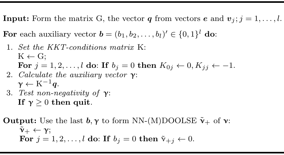 \n",
"\n",
"$~$\n",
">$\n",
"\\qquad \\mathbf{q} = \n",
"\\left(\\begin{array}{c}\n",
"\\mathbf{e}' \\mathbf{e}\\\\\n",
"(\\mathbf{e}' \\mathbf{v}_{1})^2 \\\\\n",
"\\vdots \\\\\n",
"(\\mathbf{e}' \\mathbf{v}_{l})^2\n",
"\\end{array}\\right)\n",
"$\n",
">\n",
"> $\\qquad\\mathrm{G} = \\left(\\begin{array}{ccccc}\n",
"\\small\n",
"n^* & ||\\mathbf{v}_{1}||^2 & ||\\mathbf{v}_{2}||^2 & \\ldots & ||\\mathbf{v}_{l}||^2 \\\\\n",
"||\\mathbf{v}_{1}||^2 & ||\\mathbf{v}_{1}||^4 & 0 & \\ldots & 0 \\\\\n",
"||\\mathbf{v}_{2}||^2 & 0 & ||\\mathbf{v}_{2}||^4 & \\ldots & 0 \\\\\n",
"\\vdots & \\vdots & \\vdots & \\ldots & \\vdots \\\\\n",
"||\\mathbf{v}_{l}||^2 & 0 & 0 & \\ldots & ||\\mathbf{v}_{l}||^4\n",
"\\end{array}\\right)\n",
"$"
]
},
{
"cell_type": "code",
"execution_count": 13,
"metadata": {
"ExecuteTime": {
"end_time": "2019-05-19T17:02:07.457000Z",
"start_time": "2019-05-19T17:02:01.325Z"
}
},
"outputs": [],
"source": [
"NNMDOOLSE_kkt <- function(X, F, V, method = \"NNDOOLSE\") {\n",
" n_star <- length(X)\n",
" k <- ncol(F)\n",
" l <- ncol(V)\n",
" if(method == \"NNMDOOLSE\") {\n",
" n_star <- n_star - k\n",
" }\n",
" \n",
" MF <- makeM_F(F)\n",
" u <- diag(t(V) %*% V)\n",
" G <- rbind(c(n_star,u),cbind(u, diag(u^2)))\n",
" b_comb <- expand.grid(rep(list(0:1), l))\n",
" \n",
" eps <- c(MF %*% X)\n",
" q <- c(eps %*% eps, (eps %*% V)^2)\n",
" K <- G\n",
" s <- vector()\n",
" \n",
" for(i in 1:nrow(b_comb)) {\n",
" K_inv <- matrix()\n",
" b <- as.vector(unlist(b_comb[i,]))\n",
" for(j in 1:length(b)) {\n",
" if(b[j] == 0) {\n",
" K[1,j+1] <- 0\n",
" K[j+1,j+1] <- -1\n",
" }\n",
" K_inv <- solve(K)\n",
" }\n",
" beta <- c(K_inv %*% q)\n",
" if(all(beta >= 0)) {\n",
" s <- beta[1]\n",
" for(m in 1:l) {\n",
" if(b[m] == 0) {\n",
" s <- c(s, 0)\n",
" } else {\n",
" s <- c(s, beta[m+1])\n",
" }\n",
" }\n",
" break\n",
" } else {\n",
" K <- G\n",
" }\n",
" }\n",
" return(list(\"estimates\" = s, \"b\" = b))\n",
"}"
]
},
{
"cell_type": "code",
"execution_count": 14,
"metadata": {
"ExecuteTime": {
"end_time": "2019-05-19T17:02:07.545000Z",
"start_time": "2019-05-19T17:02:01.327Z"
}
},
"outputs": [
{
"name": "stdout",
"output_type": "stream",
"text": [
"[1] 0.05595104 0.02392048 0.01394113\n",
"[1] 0.06242647\n",
"[1] 1 1\n"
]
}
],
"source": [
"NN_DOOLSE <- NNMDOOLSE_kkt(x, F, V)\n",
"print(NN_DOOLSE$estimates)\n",
"print(norm_vec(NN_DOOLSE$estimates))\n",
"print(NN_DOOLSE$b)"
]
},
{
"cell_type": "markdown",
"metadata": {},
"source": [
"## CVXR\n",
"\n",
"nonnegative DOOLSE as a convex optimization problem\n",
"\n",
">$\n",
"\\begin{array}{ll} \n",
"\\textit{minimize} & f_0(\\boldsymbol{\\nu})=||\\mathbf{e}\\mathbf{e}'-\\Sigma_\\boldsymbol{\\nu}||^2 \\\\[6pt]\n",
"\\textit{subject to} & \\boldsymbol{\\nu} = \\left(\\nu_0, \\ldots, \\nu_l\\right)'\\in [0, \\infty)^{l+1} \n",
"\\end{array}\n",
"$"
]
},
{
"cell_type": "code",
"execution_count": 15,
"metadata": {
"ExecuteTime": {
"end_time": "2019-05-19T17:02:07.584000Z",
"start_time": "2019-05-19T17:02:01.330Z"
},
"scrolled": true
},
"outputs": [],
"source": [
"NNDOOLSE_CVXR <- function(X, F, V) {\n",
" n <- length(X)\n",
" k <- ncol(F)\n",
" l <- ncol(V)\n",
"\n",
" # GF <- t(F) %*% F\n",
" # InvGF <- solve(GF)\n",
" I <- diag(n)\n",
" # PF <- F %*% InvGF %*% t(F)\n",
" #MF <- I - PF\n",
" MF <- makeM_F(F)\n",
" MFV <- MF %*% V\n",
"\n",
" SX <- MF %*% X %*% t(X) %*% MF\n",
" s <- Variable(l+1)\n",
" p_obj <- Minimize(sum_squares(SX - (s[1] %*% I) - (V %*% diag(s[2:(l+1)]) %*% t(V))))\n",
" constr <- list(s >= 0)\n",
" prob <- Problem(p_obj, constr)\n",
"\n",
" sol <- solve(prob)\n",
"\n",
" return(as.vector(sol$getValue(s)))\n",
"}"
]
},
{
"cell_type": "code",
"execution_count": 16,
"metadata": {
"ExecuteTime": {
"end_time": "2019-05-19T17:02:08.938000Z",
"start_time": "2019-05-19T17:02:01.335Z"
}
},
"outputs": [
{
"name": "stdout",
"output_type": "stream",
"text": [
"[1] 0.05595096 0.02392044 0.01394109\n",
"[1] 0.06242637\n"
]
}
],
"source": [
"NN_DOOLSEcvxr <- NNDOOLSE_CVXR(x, F, V)\n",
"print(NN_DOOLSEcvxr)\n",
"print(norm_vec(NN_DOOLSEcvxr))"
]
},
{
"cell_type": "markdown",
"metadata": {},
"source": [
"## CVXR\n",
"\n",
"using equivalent (RE)MLE convex problem (proposition 5, _Hancova et al 2019_)\n",
"\n",
"\n",
">$\n",
"\\begin{array}{ll} \n",
"\\textit{minimize} & \\quad f_0(\\mathbf{d})=-(n^*\\!-l)\\ln d_0 - \\displaystyle\\sum\\limits_{j=1}^{l} \n",
"\t\t\\ln(d_0-d_j||\\mathbf{v}_j||^2+d_0\\mathbf{e}'\\mathbf{e}-\\mathbf{e}'\\mathrm{V}\\,\\mathrm{diag}\\{d_j\\}\\mathrm{V}'\\mathbf{e} \\\\[6pt]\n",
"\\textit{subject to} & \\quad d_0 > \\max\\{d_j||\\mathbf{v}_j||^2, j = 1, \\ldots, l\\} \\\\\n",
" & \\quad d_j \\geq 0, j=1,\\ldots l \\\\\n",
" & \\\\\n",
"& \\quad\\text{for MLE: } n^* = n, \\text{ for REMLE: } n^* = n-k \\\\\n",
"\\textit{back transformation:} & \\quad \\nu_0 = \\dfrac{1}{d_0}, \\nu_j = \\dfrac{d_j}{d_0\\left(d_0 -d_j||\\mathbf{v}_j||^2\\right)}\n",
"\\end{array}\n",
"$"
]
},
{
"cell_type": "code",
"execution_count": 17,
"metadata": {
"ExecuteTime": {
"end_time": "2019-05-19T17:02:08.973000Z",
"start_time": "2019-05-19T17:02:01.339Z"
}
},
"outputs": [],
"source": [
"MLE_CVXR <- function(X, F, V){\n",
"\n",
" n <- length(X)\n",
" l <- ncol(V)\n",
"\n",
" MF <- makeM_F(F)\n",
" GV <- t(V) %*% V\n",
" p <- n - l\n",
"\n",
" e <- as.vector(MF %*% X)\n",
" ee <- as.numeric(t(e) %*% e)\n",
" eV <- t(e) %*% V\n",
" Ve <- t(V) %*% e\n",
" d <- Variable(l+1)\n",
" logdetS <- p * log(d[1]) + sum(log(d[1] - GV %*% d[2:(l+1)]))\n",
" obj <- Maximize(logdetS - ((d[1] * ee) - (eV %*% diag(d[2:(l+1)]) %*% Ve)))\n",
" constr <- list(d[2:(l+1)] >= 0, d[1] >= max_entries(GV %*% d[2:(l+1)]))\n",
" p_MLE <- Problem(obj, constr)\n",
"\n",
" sol <- solve(p_MLE)\n",
"\n",
" s <- 1 / sol$getValue(d)[1]\n",
" sj <- vector()\n",
" for(j in 2:(l+1)) {\n",
" sj <- c(sj, sol$getValue(d)[j]/(sol$getValue(d)[1] * (sol$getValue(d)[1] - sol$getValue(d)[j] * GV[j-1,j-1])))\n",
" }\n",
" result <- c(s, sj)\n",
"\n",
" return(as.vector(result))\n",
"\n",
"}"
]
},
{
"cell_type": "code",
"execution_count": 18,
"metadata": {
"ExecuteTime": {
"end_time": "2019-05-19T17:02:13.110000Z",
"start_time": "2019-05-19T17:02:01.342Z"
}
},
"outputs": [
{
"name": "stdout",
"output_type": "stream",
"text": [
"[1] 0.05595104 0.02392050 0.01394115\n",
"[1] 0.06242648\n"
]
}
],
"source": [
"MLEcvxr <- MLE_CVXR(x, F, V)\n",
"print(MLEcvxr)\n",
"print(norm_vec(MLEcvxr))"
]
},
{
"cell_type": "markdown",
"metadata": {},
"source": [
"## $\\boldsymbol{2^{nd}}$ stage of EBLUP-NE"
]
},
{
"cell_type": "code",
"execution_count": 19,
"metadata": {
"ExecuteTime": {
"end_time": "2019-05-19T17:02:13.156000Z",
"start_time": "2019-05-19T17:02:01.345Z"
}
},
"outputs": [
{
"name": "stdout",
"output_type": "stream",
"text": [
"[1] 1.0000000 0.8817033 0.8094585\n"
]
}
],
"source": [
"# numerical results\n",
"print(rho2(NN_DOOLSE$estimates))"
]
},
{
"cell_type": "code",
"execution_count": 20,
"metadata": {
"ExecuteTime": {
"end_time": "2019-05-19T17:02:13.198000Z",
"start_time": "2019-05-19T17:02:01.348Z"
}
},
"outputs": [
{
"name": "stdout",
"output_type": "stream",
"text": [
"[1] 0.05934201 0.02246111 0.01254283\n",
"[1] 0.06467842\n"
]
}
],
"source": [
"print(EBLUPNE(NN_DOOLSE$estimates)) \n",
"print(norm_vec(EBLUPNE(NN_DOOLSE$estimates)))"
]
},
{
"cell_type": "markdown",
"metadata": {},
"source": [
"***\n",
"\n",
"# NN-DOOLSE or REMLE\n",
"using the KKT algorithm (tab.3, _Hancova et al 2019_)\n",
"\n",
"## $\\boldsymbol{1^{st}}$ stage of EBLUP-NE "
]
},
{
"cell_type": "markdown",
"metadata": {},
"source": [
"## KKT algorithm"
]
},
{
"cell_type": "code",
"execution_count": 21,
"metadata": {
"ExecuteTime": {
"end_time": "2019-05-19T17:02:13.237000Z",
"start_time": "2019-05-19T17:02:01.351Z"
}
},
"outputs": [],
"source": [
"NN_MDOOLSE <- NNMDOOLSE_kkt(x, F, V, method = \"NNMDOOLSE\")"
]
},
{
"cell_type": "code",
"execution_count": 22,
"metadata": {
"ExecuteTime": {
"end_time": "2019-05-19T17:02:13.279000Z",
"start_time": "2019-05-19T17:02:01.354Z"
}
},
"outputs": [
{
"name": "stdout",
"output_type": "stream",
"text": [
"[1] 0.05934201 0.02382629 0.01384694\n",
"[1] 0.06542862\n",
"[1] 1 1\n"
]
}
],
"source": [
"print(NN_MDOOLSE$estimates)\n",
"print(norm_vec(NN_MDOOLSE$estimates))\n",
"print(NN_MDOOLSE$b)"
]
},
{
"cell_type": "markdown",
"metadata": {},
"source": [
"## CVXR\n",
"\n",
"nonnegative DOOLSE as a convex optimization problem\n",
"\n",
">$\n",
"\\begin{array}{ll} \n",
"\\textit{minimize} & f_0(\\boldsymbol{\\nu})=||\\mathbf{e}\\mathbf{e}'-\\mathrm{M_F}\\Sigma_\\boldsymbol{\\nu}\\mathrm{M_F}||^2 \\\\[6pt]\n",
"\\textit{subject to} & \\boldsymbol{\\nu} = \\left(\\nu_0, \\ldots, \\nu_l\\right)'\\in [0, \\infty)^{l+1} \n",
"\\end{array}\n",
"$"
]
},
{
"cell_type": "code",
"execution_count": 23,
"metadata": {
"ExecuteTime": {
"end_time": "2019-05-19T17:02:13.315000Z",
"start_time": "2019-05-19T17:02:01.356Z"
}
},
"outputs": [],
"source": [
"NNMDOOLSE_CVXR <- function(X, F, V) {\n",
" n <- length(X)\n",
" k <- ncol(F)\n",
" l <- ncol(V)\n",
"\n",
" # GF <- t(F) %*% F\n",
" # InvGF <- solve(GF)\n",
" I <- diag(n)\n",
" # PF <- F %*% InvGF %*% t(F)\n",
" #MF <- I - PF\n",
" MF <- makeM_F(F)\n",
" MFV <- MF %*% V\n",
"\n",
" SX <- MF %*% X %*% t(X) %*% MF\n",
" s <- Variable(l+1)\n",
" p_obj <- Minimize(sum_squares(SX - (s[1] %*% MF) - (MFV %*% diag(s[2:(l+1)]) %*% t(MFV))))\n",
" constr <- list(s >= 0)\n",
" prob <- Problem(p_obj, constr)\n",
"\n",
" sol <- solve(prob)\n",
"\n",
" return(as.vector(sol$getValue(s)))\n",
"}"
]
},
{
"cell_type": "code",
"execution_count": 24,
"metadata": {
"ExecuteTime": {
"end_time": "2019-05-19T17:02:14.668000Z",
"start_time": "2019-05-19T17:02:01.359Z"
}
},
"outputs": [
{
"name": "stdout",
"output_type": "stream",
"text": [
"[1] 0.05934192 0.02382624 0.01384690\n",
"[1] 0.06542851\n"
]
}
],
"source": [
"NN_MDOOLSEcvxr <- NNMDOOLSE_CVXR(x, F, V)\n",
"print(NN_MDOOLSEcvxr)\n",
"print(norm_vec(NN_MDOOLSEcvxr))"
]
},
{
"cell_type": "markdown",
"metadata": {},
"source": [
"## CVXR\n",
"\n",
"using equivalent (RE)MLE convex problem (proposition 5, _Hancova et al 2019_)\n",
"\n",
"\n",
">$\n",
"\\begin{array}{ll} \n",
"\\textit{minimize} & \\quad f_0(\\mathbf{d})=-(n^*\\!-l)\\ln d_0 - \\displaystyle\\sum\\limits_{j=1}^{l} \n",
"\t\t\\ln(d_0-d_j||\\mathbf{v}_j||^2+d_0\\mathbf{e}'\\mathbf{e}-\\mathbf{e}'\\mathrm{V}\\,\\mathrm{diag}\\{d_j\\}\\mathrm{V}'\\mathbf{e} \\\\[6pt]\n",
"\\textit{subject to} & \\quad d_0 > \\max\\{d_j||\\mathbf{v}_j||^2, j = 1, \\ldots, l\\} \\\\\n",
" & \\quad d_j \\geq 0, j=1,\\ldots l \\\\\n",
" & \\\\\n",
"& \\quad\\text{for MLE: } n^* = n, \\text{ for REMLE: } n^* = n-k \\\\\n",
"\\textit{back transformation:} & \\quad \\nu_0 = \\dfrac{1}{d_0}, \\nu_j = \\dfrac{d_j}{d_0\\left(d_0 -d_j||\\mathbf{v}_j||^2\\right)}\n",
"\\end{array}\n",
"$"
]
},
{
"cell_type": "code",
"execution_count": 25,
"metadata": {
"ExecuteTime": {
"end_time": "2019-05-19T17:02:14.712000Z",
"start_time": "2019-05-19T17:02:01.361Z"
}
},
"outputs": [],
"source": [
"REMLE_CVXR <- function(X, F, V){\n",
"\n",
" n <- length(X)\n",
" k <- ncol(F)\n",
" l <- ncol(V)\n",
"\n",
" MF <- makeM_F(F)\n",
" GV <- t(V) %*% V\n",
" p <- n - l - k\n",
"\n",
" e <- as.vector(MF %*% X)\n",
" ee <- as.numeric(t(e) %*% e)\n",
" eV <- t(e) %*% V\n",
" Ve <- t(V) %*% e\n",
" d <- Variable(l+1)\n",
" logdetS <- p * log(d[1]) + sum(log(d[1] - GV %*% d[2:(l+1)]))\n",
" obj <- Maximize(logdetS - ((d[1] * ee) - (eV %*% diag(d[2:(l+1)]) %*% Ve)))\n",
" constr <- list(d[2:(l+1)] >= 0, d[1] >= max_entries(GV %*% d[2:(l+1)]))\n",
" p_remle <- Problem(obj, constr)\n",
"\n",
" sol <- solve(p_remle)\n",
"\n",
" s <- 1 / sol$getValue(d)[1]\n",
" sj <- vector()\n",
" for(j in 2:(l+1)) {\n",
" sj <- c(sj, sol$getValue(d)[j]/(sol$getValue(d)[1] * (sol$getValue(d)[1] - sol$getValue(d)[j] * GV[j-1,j-1])))\n",
" }\n",
"\n",
" result <- c(s, sj)\n",
"\n",
" return(as.vector(result))\n",
"}"
]
},
{
"cell_type": "code",
"execution_count": 26,
"metadata": {
"ExecuteTime": {
"end_time": "2019-05-19T17:02:18.653000Z",
"start_time": "2019-05-19T17:02:01.364Z"
}
},
"outputs": [
{
"name": "stdout",
"output_type": "stream",
"text": [
"[1] 0.05934201 0.02382629 0.01384695\n",
"[1] 0.06542862\n"
]
}
],
"source": [
"REMLEcvxr <- REMLE_CVXR(x, F, V)\n",
"print(REMLEcvxr)\n",
"print(norm_vec(REMLEcvxr))"
]
},
{
"cell_type": "markdown",
"metadata": {},
"source": [
"## $\\boldsymbol{2^{nd}}$ stage of EBLUP-NE"
]
},
{
"cell_type": "code",
"execution_count": 27,
"metadata": {
"ExecuteTime": {
"end_time": "2019-05-19T17:02:18.689000Z",
"start_time": "2019-05-19T17:02:01.366Z"
}
},
"outputs": [
{
"name": "stdout",
"output_type": "stream",
"text": [
"[1] 1.0000000 0.8747730 0.7985572\n"
]
}
],
"source": [
"# numerical results\n",
"print(rho2(NN_MDOOLSE$estimates))"
]
},
{
"cell_type": "code",
"execution_count": 28,
"metadata": {
"ExecuteTime": {
"end_time": "2019-05-19T17:02:18.724000Z",
"start_time": "2019-05-19T17:02:01.369Z"
}
},
"outputs": [
{
"name": "stdout",
"output_type": "stream",
"text": [
"[1] 0.05934201 0.02228456 0.01237391\n",
"[1] 0.06458475\n"
]
}
],
"source": [
"print(EBLUPNE(NN_MDOOLSE$estimates)) \n",
"print(norm_vec(EBLUPNE(NN_MDOOLSE$estimates)))"
]
},
{
"cell_type": "markdown",
"metadata": {},
"source": [
"***\n",
"\n",
"# References \n",
"This notebook belongs to suplementary materials of the paper submitted to Statistical Papers and available at .\n",
"\n",
"* Hančová, M., Vozáriková, G., Gajdoš, A., Hanč, J. (2019). [Estimating variance components in time series\n",
"\tlinear regression models using empirical BLUPs and convex optimization](https://arxiv.org/abs/1905.07771), https://arxiv.org/, 2019.\n",
"\n",
"### Abstract of the paper\n",
"\n",
"We propose a two-stage estimation method of variance components in time series models known as FDSLRMs, whose observations can be described by a linear mixed model (LMM). We based estimating variances, fundamental quantities in a time series forecasting approach called kriging, on the empirical (plug-in) best linear unbiased predictions of unobservable random components in FDSLRM. \n",
"\n",
"The method, providing invariant non-negative quadratic estimators, can be used for any absolutely continuous probability distribution of time series data. As a result of applying the convex optimization and the LMM methodology, we resolved two problems $-$ theoretical existence and equivalence between least squares estimators, non-negative (M)DOOLSE, and maximum likelihood estimators, (RE)MLE, as possible starting points of our method and a \n",
"practical lack of computational implementation for FDSLRM. As for computing (RE)MLE in the case of $ n $ observed time series values, we also discovered a new algorithm of order $\\mathcal{O}(n)$, which at the default precision is $10^7$ times more accurate and $n^2$ times faster than the best current Python(or R)-based computational packages, namely CVXPY, CVXR, nlme, sommer and mixed. \n",
"\n",
"We illustrate our results on three real data sets $-$ electricity consumption, tourism and cyber security $-$ which are easily available, reproducible, sharable and modifiable in the form of interactive Jupyter notebooks."
]
},
{
"cell_type": "markdown",
"metadata": {},
"source": [
"* Sokol P., Gajdoš, A. (2017). [Prediction of Attacks Against Honeynet Based on Time Series Modeling](https://www.springer.com/gp/book/9783319676203). Silhavy, R., Silhavy, P., & Prokopova, Z. (Eds.). (2017). _Applied Computational Intelligence and Mathematical Methods (Vol. 662)_. Cham: Springer International Publishing, pp. 360-371"
]
},
{
"cell_type": "markdown",
"metadata": {},
"source": [
"| [Table of Contents](#table_of_contents) | [Data and model](#data_and_model) | [Natural estimators](#natural_estimators) | [NN-DOOLSE, MLE](#doolse) | [NN-MDOOLSE, REMLE](#mdoolse) | [References](#references) |"
]
}
],
"metadata": {
"kernelspec": {
"display_name": "R",
"language": "R",
"name": "ir"
},
"language_info": {
"codemirror_mode": "r",
"file_extension": ".r",
"mimetype": "text/x-r-source",
"name": "R",
"pygments_lexer": "r",
"version": "3.5.1"
},
"latex_envs": {
"LaTeX_envs_menu_present": true,
"autoclose": false,
"autocomplete": true,
"bibliofile": "biblio.bib",
"cite_by": "apalike",
"current_citInitial": 1,
"eqLabelWithNumbers": true,
"eqNumInitial": 1,
"hotkeys": {
"equation": "Ctrl-E",
"itemize": "Ctrl-I"
},
"labels_anchors": false,
"latex_user_defs": false,
"report_style_numbering": false,
"user_envs_cfg": false
},
"varInspector": {
"cols": {
"lenName": 16,
"lenType": 16,
"lenVar": 40
},
"kernels_config": {
"python": {
"delete_cmd_postfix": "",
"delete_cmd_prefix": "del ",
"library": "var_list.py",
"varRefreshCmd": "print(var_dic_list())"
},
"r": {
"delete_cmd_postfix": ") ",
"delete_cmd_prefix": "rm(",
"library": "var_list.r",
"varRefreshCmd": "cat(var_dic_list()) "
}
},
"types_to_exclude": [
"module",
"function",
"builtin_function_or_method",
"instance",
"_Feature"
],
"window_display": false
}
},
"nbformat": 4,
"nbformat_minor": 1
}
\n",
"\n",
"$~$\n",
">$\n",
"\\qquad \\mathbf{q} = \n",
"\\left(\\begin{array}{c}\n",
"\\mathbf{e}' \\mathbf{e}\\\\\n",
"(\\mathbf{e}' \\mathbf{v}_{1})^2 \\\\\n",
"\\vdots \\\\\n",
"(\\mathbf{e}' \\mathbf{v}_{l})^2\n",
"\\end{array}\\right)\n",
"$\n",
">\n",
"> $\\qquad\\mathrm{G} = \\left(\\begin{array}{ccccc}\n",
"\\small\n",
"n^* & ||\\mathbf{v}_{1}||^2 & ||\\mathbf{v}_{2}||^2 & \\ldots & ||\\mathbf{v}_{l}||^2 \\\\\n",
"||\\mathbf{v}_{1}||^2 & ||\\mathbf{v}_{1}||^4 & 0 & \\ldots & 0 \\\\\n",
"||\\mathbf{v}_{2}||^2 & 0 & ||\\mathbf{v}_{2}||^4 & \\ldots & 0 \\\\\n",
"\\vdots & \\vdots & \\vdots & \\ldots & \\vdots \\\\\n",
"||\\mathbf{v}_{l}||^2 & 0 & 0 & \\ldots & ||\\mathbf{v}_{l}||^4\n",
"\\end{array}\\right)\n",
"$"
]
},
{
"cell_type": "code",
"execution_count": 13,
"metadata": {
"ExecuteTime": {
"end_time": "2019-05-19T17:02:07.457000Z",
"start_time": "2019-05-19T17:02:01.325Z"
}
},
"outputs": [],
"source": [
"NNMDOOLSE_kkt <- function(X, F, V, method = \"NNDOOLSE\") {\n",
" n_star <- length(X)\n",
" k <- ncol(F)\n",
" l <- ncol(V)\n",
" if(method == \"NNMDOOLSE\") {\n",
" n_star <- n_star - k\n",
" }\n",
" \n",
" MF <- makeM_F(F)\n",
" u <- diag(t(V) %*% V)\n",
" G <- rbind(c(n_star,u),cbind(u, diag(u^2)))\n",
" b_comb <- expand.grid(rep(list(0:1), l))\n",
" \n",
" eps <- c(MF %*% X)\n",
" q <- c(eps %*% eps, (eps %*% V)^2)\n",
" K <- G\n",
" s <- vector()\n",
" \n",
" for(i in 1:nrow(b_comb)) {\n",
" K_inv <- matrix()\n",
" b <- as.vector(unlist(b_comb[i,]))\n",
" for(j in 1:length(b)) {\n",
" if(b[j] == 0) {\n",
" K[1,j+1] <- 0\n",
" K[j+1,j+1] <- -1\n",
" }\n",
" K_inv <- solve(K)\n",
" }\n",
" beta <- c(K_inv %*% q)\n",
" if(all(beta >= 0)) {\n",
" s <- beta[1]\n",
" for(m in 1:l) {\n",
" if(b[m] == 0) {\n",
" s <- c(s, 0)\n",
" } else {\n",
" s <- c(s, beta[m+1])\n",
" }\n",
" }\n",
" break\n",
" } else {\n",
" K <- G\n",
" }\n",
" }\n",
" return(list(\"estimates\" = s, \"b\" = b))\n",
"}"
]
},
{
"cell_type": "code",
"execution_count": 14,
"metadata": {
"ExecuteTime": {
"end_time": "2019-05-19T17:02:07.545000Z",
"start_time": "2019-05-19T17:02:01.327Z"
}
},
"outputs": [
{
"name": "stdout",
"output_type": "stream",
"text": [
"[1] 0.05595104 0.02392048 0.01394113\n",
"[1] 0.06242647\n",
"[1] 1 1\n"
]
}
],
"source": [
"NN_DOOLSE <- NNMDOOLSE_kkt(x, F, V)\n",
"print(NN_DOOLSE$estimates)\n",
"print(norm_vec(NN_DOOLSE$estimates))\n",
"print(NN_DOOLSE$b)"
]
},
{
"cell_type": "markdown",
"metadata": {},
"source": [
"## CVXR\n",
"\n",
"nonnegative DOOLSE as a convex optimization problem\n",
"\n",
">$\n",
"\\begin{array}{ll} \n",
"\\textit{minimize} & f_0(\\boldsymbol{\\nu})=||\\mathbf{e}\\mathbf{e}'-\\Sigma_\\boldsymbol{\\nu}||^2 \\\\[6pt]\n",
"\\textit{subject to} & \\boldsymbol{\\nu} = \\left(\\nu_0, \\ldots, \\nu_l\\right)'\\in [0, \\infty)^{l+1} \n",
"\\end{array}\n",
"$"
]
},
{
"cell_type": "code",
"execution_count": 15,
"metadata": {
"ExecuteTime": {
"end_time": "2019-05-19T17:02:07.584000Z",
"start_time": "2019-05-19T17:02:01.330Z"
},
"scrolled": true
},
"outputs": [],
"source": [
"NNDOOLSE_CVXR <- function(X, F, V) {\n",
" n <- length(X)\n",
" k <- ncol(F)\n",
" l <- ncol(V)\n",
"\n",
" # GF <- t(F) %*% F\n",
" # InvGF <- solve(GF)\n",
" I <- diag(n)\n",
" # PF <- F %*% InvGF %*% t(F)\n",
" #MF <- I - PF\n",
" MF <- makeM_F(F)\n",
" MFV <- MF %*% V\n",
"\n",
" SX <- MF %*% X %*% t(X) %*% MF\n",
" s <- Variable(l+1)\n",
" p_obj <- Minimize(sum_squares(SX - (s[1] %*% I) - (V %*% diag(s[2:(l+1)]) %*% t(V))))\n",
" constr <- list(s >= 0)\n",
" prob <- Problem(p_obj, constr)\n",
"\n",
" sol <- solve(prob)\n",
"\n",
" return(as.vector(sol$getValue(s)))\n",
"}"
]
},
{
"cell_type": "code",
"execution_count": 16,
"metadata": {
"ExecuteTime": {
"end_time": "2019-05-19T17:02:08.938000Z",
"start_time": "2019-05-19T17:02:01.335Z"
}
},
"outputs": [
{
"name": "stdout",
"output_type": "stream",
"text": [
"[1] 0.05595096 0.02392044 0.01394109\n",
"[1] 0.06242637\n"
]
}
],
"source": [
"NN_DOOLSEcvxr <- NNDOOLSE_CVXR(x, F, V)\n",
"print(NN_DOOLSEcvxr)\n",
"print(norm_vec(NN_DOOLSEcvxr))"
]
},
{
"cell_type": "markdown",
"metadata": {},
"source": [
"## CVXR\n",
"\n",
"using equivalent (RE)MLE convex problem (proposition 5, _Hancova et al 2019_)\n",
"\n",
"\n",
">$\n",
"\\begin{array}{ll} \n",
"\\textit{minimize} & \\quad f_0(\\mathbf{d})=-(n^*\\!-l)\\ln d_0 - \\displaystyle\\sum\\limits_{j=1}^{l} \n",
"\t\t\\ln(d_0-d_j||\\mathbf{v}_j||^2+d_0\\mathbf{e}'\\mathbf{e}-\\mathbf{e}'\\mathrm{V}\\,\\mathrm{diag}\\{d_j\\}\\mathrm{V}'\\mathbf{e} \\\\[6pt]\n",
"\\textit{subject to} & \\quad d_0 > \\max\\{d_j||\\mathbf{v}_j||^2, j = 1, \\ldots, l\\} \\\\\n",
" & \\quad d_j \\geq 0, j=1,\\ldots l \\\\\n",
" & \\\\\n",
"& \\quad\\text{for MLE: } n^* = n, \\text{ for REMLE: } n^* = n-k \\\\\n",
"\\textit{back transformation:} & \\quad \\nu_0 = \\dfrac{1}{d_0}, \\nu_j = \\dfrac{d_j}{d_0\\left(d_0 -d_j||\\mathbf{v}_j||^2\\right)}\n",
"\\end{array}\n",
"$"
]
},
{
"cell_type": "code",
"execution_count": 17,
"metadata": {
"ExecuteTime": {
"end_time": "2019-05-19T17:02:08.973000Z",
"start_time": "2019-05-19T17:02:01.339Z"
}
},
"outputs": [],
"source": [
"MLE_CVXR <- function(X, F, V){\n",
"\n",
" n <- length(X)\n",
" l <- ncol(V)\n",
"\n",
" MF <- makeM_F(F)\n",
" GV <- t(V) %*% V\n",
" p <- n - l\n",
"\n",
" e <- as.vector(MF %*% X)\n",
" ee <- as.numeric(t(e) %*% e)\n",
" eV <- t(e) %*% V\n",
" Ve <- t(V) %*% e\n",
" d <- Variable(l+1)\n",
" logdetS <- p * log(d[1]) + sum(log(d[1] - GV %*% d[2:(l+1)]))\n",
" obj <- Maximize(logdetS - ((d[1] * ee) - (eV %*% diag(d[2:(l+1)]) %*% Ve)))\n",
" constr <- list(d[2:(l+1)] >= 0, d[1] >= max_entries(GV %*% d[2:(l+1)]))\n",
" p_MLE <- Problem(obj, constr)\n",
"\n",
" sol <- solve(p_MLE)\n",
"\n",
" s <- 1 / sol$getValue(d)[1]\n",
" sj <- vector()\n",
" for(j in 2:(l+1)) {\n",
" sj <- c(sj, sol$getValue(d)[j]/(sol$getValue(d)[1] * (sol$getValue(d)[1] - sol$getValue(d)[j] * GV[j-1,j-1])))\n",
" }\n",
" result <- c(s, sj)\n",
"\n",
" return(as.vector(result))\n",
"\n",
"}"
]
},
{
"cell_type": "code",
"execution_count": 18,
"metadata": {
"ExecuteTime": {
"end_time": "2019-05-19T17:02:13.110000Z",
"start_time": "2019-05-19T17:02:01.342Z"
}
},
"outputs": [
{
"name": "stdout",
"output_type": "stream",
"text": [
"[1] 0.05595104 0.02392050 0.01394115\n",
"[1] 0.06242648\n"
]
}
],
"source": [
"MLEcvxr <- MLE_CVXR(x, F, V)\n",
"print(MLEcvxr)\n",
"print(norm_vec(MLEcvxr))"
]
},
{
"cell_type": "markdown",
"metadata": {},
"source": [
"## $\\boldsymbol{2^{nd}}$ stage of EBLUP-NE"
]
},
{
"cell_type": "code",
"execution_count": 19,
"metadata": {
"ExecuteTime": {
"end_time": "2019-05-19T17:02:13.156000Z",
"start_time": "2019-05-19T17:02:01.345Z"
}
},
"outputs": [
{
"name": "stdout",
"output_type": "stream",
"text": [
"[1] 1.0000000 0.8817033 0.8094585\n"
]
}
],
"source": [
"# numerical results\n",
"print(rho2(NN_DOOLSE$estimates))"
]
},
{
"cell_type": "code",
"execution_count": 20,
"metadata": {
"ExecuteTime": {
"end_time": "2019-05-19T17:02:13.198000Z",
"start_time": "2019-05-19T17:02:01.348Z"
}
},
"outputs": [
{
"name": "stdout",
"output_type": "stream",
"text": [
"[1] 0.05934201 0.02246111 0.01254283\n",
"[1] 0.06467842\n"
]
}
],
"source": [
"print(EBLUPNE(NN_DOOLSE$estimates)) \n",
"print(norm_vec(EBLUPNE(NN_DOOLSE$estimates)))"
]
},
{
"cell_type": "markdown",
"metadata": {},
"source": [
"***\n",
"\n",
"# NN-DOOLSE or REMLE\n",
"using the KKT algorithm (tab.3, _Hancova et al 2019_)\n",
"\n",
"## $\\boldsymbol{1^{st}}$ stage of EBLUP-NE "
]
},
{
"cell_type": "markdown",
"metadata": {},
"source": [
"## KKT algorithm"
]
},
{
"cell_type": "code",
"execution_count": 21,
"metadata": {
"ExecuteTime": {
"end_time": "2019-05-19T17:02:13.237000Z",
"start_time": "2019-05-19T17:02:01.351Z"
}
},
"outputs": [],
"source": [
"NN_MDOOLSE <- NNMDOOLSE_kkt(x, F, V, method = \"NNMDOOLSE\")"
]
},
{
"cell_type": "code",
"execution_count": 22,
"metadata": {
"ExecuteTime": {
"end_time": "2019-05-19T17:02:13.279000Z",
"start_time": "2019-05-19T17:02:01.354Z"
}
},
"outputs": [
{
"name": "stdout",
"output_type": "stream",
"text": [
"[1] 0.05934201 0.02382629 0.01384694\n",
"[1] 0.06542862\n",
"[1] 1 1\n"
]
}
],
"source": [
"print(NN_MDOOLSE$estimates)\n",
"print(norm_vec(NN_MDOOLSE$estimates))\n",
"print(NN_MDOOLSE$b)"
]
},
{
"cell_type": "markdown",
"metadata": {},
"source": [
"## CVXR\n",
"\n",
"nonnegative DOOLSE as a convex optimization problem\n",
"\n",
">$\n",
"\\begin{array}{ll} \n",
"\\textit{minimize} & f_0(\\boldsymbol{\\nu})=||\\mathbf{e}\\mathbf{e}'-\\mathrm{M_F}\\Sigma_\\boldsymbol{\\nu}\\mathrm{M_F}||^2 \\\\[6pt]\n",
"\\textit{subject to} & \\boldsymbol{\\nu} = \\left(\\nu_0, \\ldots, \\nu_l\\right)'\\in [0, \\infty)^{l+1} \n",
"\\end{array}\n",
"$"
]
},
{
"cell_type": "code",
"execution_count": 23,
"metadata": {
"ExecuteTime": {
"end_time": "2019-05-19T17:02:13.315000Z",
"start_time": "2019-05-19T17:02:01.356Z"
}
},
"outputs": [],
"source": [
"NNMDOOLSE_CVXR <- function(X, F, V) {\n",
" n <- length(X)\n",
" k <- ncol(F)\n",
" l <- ncol(V)\n",
"\n",
" # GF <- t(F) %*% F\n",
" # InvGF <- solve(GF)\n",
" I <- diag(n)\n",
" # PF <- F %*% InvGF %*% t(F)\n",
" #MF <- I - PF\n",
" MF <- makeM_F(F)\n",
" MFV <- MF %*% V\n",
"\n",
" SX <- MF %*% X %*% t(X) %*% MF\n",
" s <- Variable(l+1)\n",
" p_obj <- Minimize(sum_squares(SX - (s[1] %*% MF) - (MFV %*% diag(s[2:(l+1)]) %*% t(MFV))))\n",
" constr <- list(s >= 0)\n",
" prob <- Problem(p_obj, constr)\n",
"\n",
" sol <- solve(prob)\n",
"\n",
" return(as.vector(sol$getValue(s)))\n",
"}"
]
},
{
"cell_type": "code",
"execution_count": 24,
"metadata": {
"ExecuteTime": {
"end_time": "2019-05-19T17:02:14.668000Z",
"start_time": "2019-05-19T17:02:01.359Z"
}
},
"outputs": [
{
"name": "stdout",
"output_type": "stream",
"text": [
"[1] 0.05934192 0.02382624 0.01384690\n",
"[1] 0.06542851\n"
]
}
],
"source": [
"NN_MDOOLSEcvxr <- NNMDOOLSE_CVXR(x, F, V)\n",
"print(NN_MDOOLSEcvxr)\n",
"print(norm_vec(NN_MDOOLSEcvxr))"
]
},
{
"cell_type": "markdown",
"metadata": {},
"source": [
"## CVXR\n",
"\n",
"using equivalent (RE)MLE convex problem (proposition 5, _Hancova et al 2019_)\n",
"\n",
"\n",
">$\n",
"\\begin{array}{ll} \n",
"\\textit{minimize} & \\quad f_0(\\mathbf{d})=-(n^*\\!-l)\\ln d_0 - \\displaystyle\\sum\\limits_{j=1}^{l} \n",
"\t\t\\ln(d_0-d_j||\\mathbf{v}_j||^2+d_0\\mathbf{e}'\\mathbf{e}-\\mathbf{e}'\\mathrm{V}\\,\\mathrm{diag}\\{d_j\\}\\mathrm{V}'\\mathbf{e} \\\\[6pt]\n",
"\\textit{subject to} & \\quad d_0 > \\max\\{d_j||\\mathbf{v}_j||^2, j = 1, \\ldots, l\\} \\\\\n",
" & \\quad d_j \\geq 0, j=1,\\ldots l \\\\\n",
" & \\\\\n",
"& \\quad\\text{for MLE: } n^* = n, \\text{ for REMLE: } n^* = n-k \\\\\n",
"\\textit{back transformation:} & \\quad \\nu_0 = \\dfrac{1}{d_0}, \\nu_j = \\dfrac{d_j}{d_0\\left(d_0 -d_j||\\mathbf{v}_j||^2\\right)}\n",
"\\end{array}\n",
"$"
]
},
{
"cell_type": "code",
"execution_count": 25,
"metadata": {
"ExecuteTime": {
"end_time": "2019-05-19T17:02:14.712000Z",
"start_time": "2019-05-19T17:02:01.361Z"
}
},
"outputs": [],
"source": [
"REMLE_CVXR <- function(X, F, V){\n",
"\n",
" n <- length(X)\n",
" k <- ncol(F)\n",
" l <- ncol(V)\n",
"\n",
" MF <- makeM_F(F)\n",
" GV <- t(V) %*% V\n",
" p <- n - l - k\n",
"\n",
" e <- as.vector(MF %*% X)\n",
" ee <- as.numeric(t(e) %*% e)\n",
" eV <- t(e) %*% V\n",
" Ve <- t(V) %*% e\n",
" d <- Variable(l+1)\n",
" logdetS <- p * log(d[1]) + sum(log(d[1] - GV %*% d[2:(l+1)]))\n",
" obj <- Maximize(logdetS - ((d[1] * ee) - (eV %*% diag(d[2:(l+1)]) %*% Ve)))\n",
" constr <- list(d[2:(l+1)] >= 0, d[1] >= max_entries(GV %*% d[2:(l+1)]))\n",
" p_remle <- Problem(obj, constr)\n",
"\n",
" sol <- solve(p_remle)\n",
"\n",
" s <- 1 / sol$getValue(d)[1]\n",
" sj <- vector()\n",
" for(j in 2:(l+1)) {\n",
" sj <- c(sj, sol$getValue(d)[j]/(sol$getValue(d)[1] * (sol$getValue(d)[1] - sol$getValue(d)[j] * GV[j-1,j-1])))\n",
" }\n",
"\n",
" result <- c(s, sj)\n",
"\n",
" return(as.vector(result))\n",
"}"
]
},
{
"cell_type": "code",
"execution_count": 26,
"metadata": {
"ExecuteTime": {
"end_time": "2019-05-19T17:02:18.653000Z",
"start_time": "2019-05-19T17:02:01.364Z"
}
},
"outputs": [
{
"name": "stdout",
"output_type": "stream",
"text": [
"[1] 0.05934201 0.02382629 0.01384695\n",
"[1] 0.06542862\n"
]
}
],
"source": [
"REMLEcvxr <- REMLE_CVXR(x, F, V)\n",
"print(REMLEcvxr)\n",
"print(norm_vec(REMLEcvxr))"
]
},
{
"cell_type": "markdown",
"metadata": {},
"source": [
"## $\\boldsymbol{2^{nd}}$ stage of EBLUP-NE"
]
},
{
"cell_type": "code",
"execution_count": 27,
"metadata": {
"ExecuteTime": {
"end_time": "2019-05-19T17:02:18.689000Z",
"start_time": "2019-05-19T17:02:01.366Z"
}
},
"outputs": [
{
"name": "stdout",
"output_type": "stream",
"text": [
"[1] 1.0000000 0.8747730 0.7985572\n"
]
}
],
"source": [
"# numerical results\n",
"print(rho2(NN_MDOOLSE$estimates))"
]
},
{
"cell_type": "code",
"execution_count": 28,
"metadata": {
"ExecuteTime": {
"end_time": "2019-05-19T17:02:18.724000Z",
"start_time": "2019-05-19T17:02:01.369Z"
}
},
"outputs": [
{
"name": "stdout",
"output_type": "stream",
"text": [
"[1] 0.05934201 0.02228456 0.01237391\n",
"[1] 0.06458475\n"
]
}
],
"source": [
"print(EBLUPNE(NN_MDOOLSE$estimates)) \n",
"print(norm_vec(EBLUPNE(NN_MDOOLSE$estimates)))"
]
},
{
"cell_type": "markdown",
"metadata": {},
"source": [
"***\n",
"\n",
"# References \n",
"This notebook belongs to suplementary materials of the paper submitted to Statistical Papers and available at .\n",
"\n",
"* Hančová, M., Vozáriková, G., Gajdoš, A., Hanč, J. (2019). [Estimating variance components in time series\n",
"\tlinear regression models using empirical BLUPs and convex optimization](https://arxiv.org/abs/1905.07771), https://arxiv.org/, 2019.\n",
"\n",
"### Abstract of the paper\n",
"\n",
"We propose a two-stage estimation method of variance components in time series models known as FDSLRMs, whose observations can be described by a linear mixed model (LMM). We based estimating variances, fundamental quantities in a time series forecasting approach called kriging, on the empirical (plug-in) best linear unbiased predictions of unobservable random components in FDSLRM. \n",
"\n",
"The method, providing invariant non-negative quadratic estimators, can be used for any absolutely continuous probability distribution of time series data. As a result of applying the convex optimization and the LMM methodology, we resolved two problems $-$ theoretical existence and equivalence between least squares estimators, non-negative (M)DOOLSE, and maximum likelihood estimators, (RE)MLE, as possible starting points of our method and a \n",
"practical lack of computational implementation for FDSLRM. As for computing (RE)MLE in the case of $ n $ observed time series values, we also discovered a new algorithm of order $\\mathcal{O}(n)$, which at the default precision is $10^7$ times more accurate and $n^2$ times faster than the best current Python(or R)-based computational packages, namely CVXPY, CVXR, nlme, sommer and mixed. \n",
"\n",
"We illustrate our results on three real data sets $-$ electricity consumption, tourism and cyber security $-$ which are easily available, reproducible, sharable and modifiable in the form of interactive Jupyter notebooks."
]
},
{
"cell_type": "markdown",
"metadata": {},
"source": [
"* Sokol P., Gajdoš, A. (2017). [Prediction of Attacks Against Honeynet Based on Time Series Modeling](https://www.springer.com/gp/book/9783319676203). Silhavy, R., Silhavy, P., & Prokopova, Z. (Eds.). (2017). _Applied Computational Intelligence and Mathematical Methods (Vol. 662)_. Cham: Springer International Publishing, pp. 360-371"
]
},
{
"cell_type": "markdown",
"metadata": {},
"source": [
"| [Table of Contents](#table_of_contents) | [Data and model](#data_and_model) | [Natural estimators](#natural_estimators) | [NN-DOOLSE, MLE](#doolse) | [NN-MDOOLSE, REMLE](#mdoolse) | [References](#references) |"
]
}
],
"metadata": {
"kernelspec": {
"display_name": "R",
"language": "R",
"name": "ir"
},
"language_info": {
"codemirror_mode": "r",
"file_extension": ".r",
"mimetype": "text/x-r-source",
"name": "R",
"pygments_lexer": "r",
"version": "3.5.1"
},
"latex_envs": {
"LaTeX_envs_menu_present": true,
"autoclose": false,
"autocomplete": true,
"bibliofile": "biblio.bib",
"cite_by": "apalike",
"current_citInitial": 1,
"eqLabelWithNumbers": true,
"eqNumInitial": 1,
"hotkeys": {
"equation": "Ctrl-E",
"itemize": "Ctrl-I"
},
"labels_anchors": false,
"latex_user_defs": false,
"report_style_numbering": false,
"user_envs_cfg": false
},
"varInspector": {
"cols": {
"lenName": 16,
"lenType": 16,
"lenVar": 40
},
"kernels_config": {
"python": {
"delete_cmd_postfix": "",
"delete_cmd_prefix": "del ",
"library": "var_list.py",
"varRefreshCmd": "print(var_dic_list())"
},
"r": {
"delete_cmd_postfix": ") ",
"delete_cmd_prefix": "rm(",
"library": "var_list.r",
"varRefreshCmd": "cat(var_dic_list()) "
}
},
"types_to_exclude": [
"module",
"function",
"builtin_function_or_method",
"instance",
"_Feature"
],
"window_display": false
}
},
"nbformat": 4,
"nbformat_minor": 1
}