{
"cells": [
{
"cell_type": "markdown",
"metadata": {},
"source": [
"| [Table of Contents](#table_of_contents) | [Data and model](#data_and_model) | [Natural estimators](#natural_estimators) | [NN-DOOLSE, MLE](#doolse) | [NN-MDOOLSE, REMLE](#mdoolse) | [References](#references) |"
]
},
{
"cell_type": "markdown",
"metadata": {},
"source": [
"**Authors:** Andrej Gajdoš, Jozef Hanč, Martina Hančová
*[Faculty of Science](https://www.upjs.sk/en/faculty-of-science/?prefferedLang=EN), P. J. Šafárik University in Košice, Slovakia*
email: [andrej.gajdos@student.upjs.sk](mailto:andrej.gajdos@student.upjs.sk)\n",
"***\n",
"** EBLUP-NE for electricity consumption 2** "
]
},
{
"cell_type": "markdown",
"metadata": {},
"source": [
" R-based computational tools - ** CVXR ** \n",
"\n",
"### Table of Contents \n",
"* [Data and model](#data_and_model) - data and model description of empirical data\n",
"* [Natural estimators](#natural_estimators) - EBLUPNE based on NE\n",
"* [NN-DOOLSE, MLE](#doolse) - EBLUPNE based on nonnegative DOOLSE (same as MLE)\n",
"* [NN-MDOOLSE, REMLE](#mdoolse) - EBLUPNE based on nonnegative MDOOLSE (same as REMLE)\n",
"* [References](#references)\n",
"\n",
"**To get back to the contents, use the Home key.**"
]
},
{
"cell_type": "markdown",
"metadata": {},
"source": [
"## R packages"
]
},
{
"cell_type": "markdown",
"metadata": {},
"source": [
"## CVXR: R-Embedded Object-Oriented Modeling Language for Convex Optimization \n",
"\n",
"* _Purpose_: R package for solving convex optimization tasks\n",
"* _Version_: 0.99-5, 2019\n",
"* _URL_: https://cvxr.rbind.io/\n",
"* _Computational parameters_ of CVXR:\n",
"> * *solver* - the convex optimization solver ECOS, OSQP, and SCS chosen according to the given problem\n",
" * **OSQP** for convex quadratic problems\n",
" * `max_iter` - maximum number of iterations (default: 4000).\n",
" * `eps_abs` - absolute accuracy (default: 1e-3).\n",
" * `eps_rel` - relative accuracy (default: 1e-4).\n",
" * **ECOS** for convex second-order cone problems \n",
" * `maxit` - maximum number of iterations (default: 100).\n",
" * `abstol` - absolute accuracy (default: 1e-8).\n",
" * `reltol` - relative accuracy (default: 1e-8).\n",
" * `feastol` - tolerance for feasibility conditions (default: 1e-8).\n",
" * `abstol_inacc` - absolute accuracy for inaccurate solution (default: 5e-5).\n",
" * `reltol_inacc` - relative accuracy for inaccurate solution (default: 5e-5).\n",
" * `feastol_inacc` - tolerance for feasibility condition for inaccurate solution (default: 1e-4).\n",
" * **SCS** for large-scale convex cone problems\n",
" * `max_iters` - maximum number of iterations (default: 5000).\n",
" * `eps` - convergence tolerance (default: 1e-5).\n",
" * `alpha` - relaxation parameter (default: 1.5).\n",
" * `scale` - factor by which the data is rescaled, only used if `normalize` is TRUE (default: 1.0).\n",
" * `normalize` - whether the heuristic data rescaling should be used (default: TRUE)."
]
},
{
"cell_type": "markdown",
"metadata": {},
"source": [
"*Important note:* \n",
"**After our testing, we found that the standard CVXR package installation, unlike a local installation using Anaconda R distribution or CRAN distribution, did not work in a Binder repository. We are intensively communicating with authors of the package to fix it. At this moment, you have to use your local installation of Jupyter with R kernel or you can see our live Binder Python notebooks using CVXPY with the same results and very similar commands.** "
]
},
{
"cell_type": "code",
"execution_count": 1,
"metadata": {
"ExecuteTime": {
"end_time": "2019-05-19T17:18:27.241000Z",
"start_time": "2019-05-19T17:18:25.600Z"
}
},
"outputs": [
{
"name": "stderr",
"output_type": "stream",
"text": [
"Warning message:\n",
"\"package 'CVXR' was built under R version 3.5.3\"\n",
"Attaching package: 'CVXR'\n",
"\n",
"The following object is masked from 'package:stats':\n",
"\n",
" power\n",
"\n"
]
}
],
"source": [
"library(CVXR)"
]
},
{
"cell_type": "markdown",
"metadata": {},
"source": [
"***\n",
"\n",
"# Data and Toy Model 2"
]
},
{
"cell_type": "markdown",
"metadata": {},
"source": [
"In this FDSLRM application, we model the econometric time series data set, representing the hours observations of the consumption of the electric energy in some department store. The number of time series observations is $n=24$. The data and model were adapted from _Štulajter & Witkovský, 2004_.\n",
"\n",
"The consumption data can be fitted by the following Gaussian orthogonal FDSLRM:\n",
"\n",
"$ \n",
"\\begin{array}{rl}\n",
"& X(t) & \\! = \\! & \\beta_1+\\beta_2\\cos\\left(\\tfrac{2\\pi t}{24}\\right)+\\beta_3\\sin\\left(\\tfrac{2\\pi t}{24}\\right) +\\\\\n",
"& & & +Y_1\\cos\\left(\\tfrac{2\\pi t\\cdot 2}{24}\\right)+Y_2\\sin\\left(\\tfrac{2\\pi t\\cdot 2}{24}\\right)+\\\\\n",
"& & & +Y_3\\cos\\left(\\tfrac{2\\pi t\\cdot 3}{24}\\right)+Y_4\\sin\\left(\\tfrac{2\\pi t\\cdot 3}{24}\\right)\n",
"+w(t), \\, t\\in \\mathbb{N},\n",
"\\end{array}\n",
"$ \n",
"\n",
"where $\\boldsymbol{\\beta}=(\\beta_1,\\,\\beta_2,\\,\\beta_3)' \\in \\mathbb{R}^3\\,,\\mathbf{Y} = (Y_1, Y_2, Y_3, Y_4)' \\sim \\mathcal{N}_4(\\boldsymbol{0}, \\mathrm{D})\\,, w(t) \\sim \\mathcal{iid}\\, \\mathcal{N} (0, \\sigma_0^2)\\,, \\boldsymbol{\\nu}= (\\sigma_0^2, \\sigma_1^2, \\sigma_2^2, \\sigma_3^2, \\sigma_4^2) \\in \\mathbb{R}_{+}^5.$ "
]
},
{
"cell_type": "code",
"execution_count": 2,
"metadata": {
"ExecuteTime": {
"end_time": "2019-05-19T17:18:27.319000Z",
"start_time": "2019-05-19T17:18:25.605Z"
}
},
"outputs": [],
"source": [
"# data - time series observation\n",
"x <- c(40.3,40.7,38.5,37.9,38.6,41.1,45.2,45.7,46.7,46.5,\n",
" 45.2,45.1,45.8,46.3,47.5,48.5,49.1,51.7,50.6,48.0,\n",
" 44.7,41.2,40.0,40.3)\n",
"t <- 1:length(x)"
]
},
{
"cell_type": "code",
"execution_count": 3,
"metadata": {
"ExecuteTime": {
"end_time": "2019-05-19T17:18:27.365000Z",
"start_time": "2019-05-19T17:18:25.607Z"
}
},
"outputs": [],
"source": [
"# auxilliary functions to create design matrices F, V and the projection matrix M_F\n",
"makeF <- function(times, freqs) {\n",
"\n",
" n <- length(times)\n",
" f <- length(freqs)\n",
" c1 <- matrix(1, n)\n",
" F <- matrix(c1, n, 1)\n",
"\n",
" for (i in 1:f) {\n",
" F <- cbind(F, cos(2 * pi * freqs[i] * times))\n",
" F <- cbind(F, sin(2 * pi * freqs[i] * times))\n",
" }\n",
"\n",
" return(F)\n",
"}\n",
"\n",
"makeV <- function(times, freqs) {\n",
"\n",
" V <- makeF(times, freqs)\n",
" V <- V[, -1]\n",
"\n",
" return(V)\n",
"}\n",
"\n",
"makeM_F <- function(F) {\n",
"\n",
" n <- nrow(F)\n",
" c1 <- rep(1, n)\n",
" I <- diag(c1)\n",
" M_F <- I - F %*% solve((t(F) %*% F)) %*% t(F)\n",
"\n",
" return(M_F)\n",
"}"
]
},
{
"cell_type": "code",
"execution_count": 4,
"metadata": {
"ExecuteTime": {
"end_time": "2019-05-19T17:18:27.427000Z",
"start_time": "2019-05-19T17:18:25.611Z"
}
},
"outputs": [],
"source": [
"# model parameters\n",
"n <- 24 \n",
"k <- 3 \n",
"l <- 4\n",
"\n",
"# model - design matrices F, V\n",
"F <- makeF(t, c(1/24))\n",
"V <- makeV(t, c(2/24, 3/24))\n",
"\n",
"# columns vj of V and their squared norm ||vj||^2\n",
"nv2 = colSums(V ^ 2)"
]
},
{
"cell_type": "code",
"execution_count": 5,
"metadata": {
"ExecuteTime": {
"end_time": "2019-05-19T17:18:27.478000Z",
"start_time": "2019-05-19T17:18:25.613Z"
}
},
"outputs": [],
"source": [
"# auxiliary matrices and vectors\n",
"\n",
"# Gram matrices GF, GV\n",
"GF <- t(F) %*% F\n",
"GV <- t(V) %*% V\n",
"InvGF <- solve(GF)\n",
"InvGV <- solve(GV)\n",
"\n",
"# projectors PF, MF, PV, MV\n",
"In <- diag(n)\n",
"PF <- F %*% InvGF %*% t(F)\n",
"PV <- V %*% InvGV %*% t(V)\n",
"MF <- In - PF\n",
"MV <- In - PV\n",
"\n",
"# residuals e\n",
"e <- MF %*% x"
]
},
{
"cell_type": "markdown",
"metadata": {},
"source": [
"***\n",
"\n",
"# Natural estimators\n",
"\n",
"## ANALYTICALLY \n",
"using formula (4.1) from _Hancova et al 2019_\n",
"\n",
">$\n",
"\\renewcommand{\\arraystretch}{1.4}\n",
"\\tilde{\\boldsymbol{\\nu}}(\\mathbf{e}) =\n",
"\\begin{pmatrix}\n",
"\\tfrac{1}{n-k-l}\\,\\mathbf{e}'\\,\\mathrm{M_V}\\,\\mathbf{e} \\\\\n",
"(\\mathbf{e}'\\mathbf{v}_1)^2/||\\mathbf{v}_1||^4 \\\\\n",
"\\vdots \\\\\n",
"(\\mathbf{e}'\\mathbf{v}_l)^2/||\\mathbf{v}_l||^4\n",
"\\end{pmatrix} \n",
"$\n",
"\n",
"## $\\boldsymbol{1^{st}}$ stage of EBLUP-NE "
]
},
{
"cell_type": "code",
"execution_count": 6,
"metadata": {
"ExecuteTime": {
"end_time": "2019-05-19T17:18:27.522000Z",
"start_time": "2019-05-19T17:18:25.616Z"
}
},
"outputs": [],
"source": [
"# auxilliary function to calculate the norm of a vector\n",
"norm_vec <- function(x) sqrt(sum(x^2))"
]
},
{
"cell_type": "code",
"execution_count": 7,
"metadata": {
"ExecuteTime": {
"end_time": "2019-05-19T17:18:27.572000Z",
"start_time": "2019-05-19T17:18:25.619Z"
}
},
"outputs": [
{
"name": "stdout",
"output_type": "stream",
"text": [
"[1] 1.093045 2.965717 1.761859 0.371935 1.863479\n",
"[1] 4.087207\n"
]
}
],
"source": [
"# NE according to formula (4.1)\n",
"NE0 <- 1/(n-k-l) * t(e) %*% MV %*% (e)\n",
"NEj <- (t(e) %*% V) ^ 2 / nv2 ^ 2\n",
"NE <- c(NE0, NEj) \n",
"print(NE)\n",
"print(norm_vec(NE))"
]
},
{
"cell_type": "markdown",
"metadata": {},
"source": [
"## CVXR\n",
"\n",
"\n",
"NE as a convex optimization problem\n",
"\n",
">$\n",
"\\begin{array}{ll} \n",
"\\textit{minimize} & \\quad \n",
"f_0(\\boldsymbol{\\nu})=||\\mathbf{e}\\mathbf{e}' - \\mathrm{VDV'}||^2+||\\mathrm{M_V}\\mathbf{e}\\mathbf{e}'\\mathrm{M_V}-\\nu_0\\mathrm{M_F}\\mathrm{M_V}||^2 \\\\[6pt]\n",
"\\textit{subject to} & \\quad \\boldsymbol{\\nu} = \\left(\\nu_0, \\ldots, \\nu_l\\right)'\\in [0, \\infty)^{l+1} \n",
"\\end{array}\n",
"$"
]
},
{
"cell_type": "code",
"execution_count": 8,
"metadata": {
"ExecuteTime": {
"end_time": "2019-05-19T17:18:30.569000Z",
"start_time": "2019-05-19T17:18:25.622Z"
}
},
"outputs": [
{
"name": "stdout",
"output_type": "stream",
"text": [
"NEcvxr = 1.093047 2.965724 1.761866 0.3719285 1.863487\n",
"norm = 4.087219"
]
}
],
"source": [
"# the optimization variable, objective function\n",
"v <- Variable(l+1) \n",
"fv <- sum_squares(e%*%t(e)-V%*%diag(v[2:(l+1)])%*%t(V)) + sum_squares(MV%*%e%*%t(e)%*%MV-v[1]%*%MF%*%MV)\n",
"\n",
"# the optimization problem for NE\n",
"objective <- Minimize(fv)\n",
"constraints <- list(v >= 0)\n",
"prob <- Problem(objective, constraints)\n",
"\n",
"# solve the NE problem\n",
"sol <- solve(prob) \n",
"cat(\"NEcvxr =\",as.vector(sol$getValue(v)))\n",
"cat(\"\\n\")\n",
"cat(\"norm =\", norm_vec(as.vector(sol$getValue(v))))"
]
},
{
"cell_type": "markdown",
"metadata": {},
"source": [
"## $\\boldsymbol{2^{nd}}$ stage of EBLUP-NE\n",
"using formula (3.9) from _Hancova et al 2019_.\n",
">$\n",
"\\mathring{\\nu}_j = \\rho_j^2 \\tilde{\\nu}_j; j = 0,1 \\ldots, l\\\\\n",
"\\rho_0 = 1, \\rho_j = \\dfrac{\\hat{\\nu}_j||\\mathbf{v}_j||^2}{\\hat{\\nu}_0+\\hat{\\nu}_j||\\mathbf{v}_j||^2} \n",
"$\n",
">\n",
">where $\\boldsymbol{\\tilde{\\nu}}$ are NE, $\\boldsymbol{\\hat{\\nu}}$ are initial estimates for EBLUP-NE"
]
},
{
"cell_type": "code",
"execution_count": 9,
"metadata": {
"ExecuteTime": {
"end_time": "2019-05-19T17:18:30.602000Z",
"start_time": "2019-05-19T17:18:25.625Z"
}
},
"outputs": [],
"source": [
"# EBLUP-NE based on formula (3.9)\n",
"rho2 <- function(est) {\n",
" result <- c(1)\n",
" for(j in 2:length(est)) {\n",
" result <- c(result, (est[j]*nv2[j-1]/(est[1]+est[j]*nv2[j-1])) ^ 2)\n",
" }\n",
" return(result)\n",
"}"
]
},
{
"cell_type": "code",
"execution_count": 10,
"metadata": {
"ExecuteTime": {
"end_time": "2019-05-19T17:18:30.641000Z",
"start_time": "2019-05-19T17:18:25.628Z"
}
},
"outputs": [],
"source": [
"EBLUPNE <- function(est) {\n",
" result <- NE * rho2(est)\n",
" return(result)\n",
" }"
]
},
{
"cell_type": "code",
"execution_count": 11,
"metadata": {
"ExecuteTime": {
"end_time": "2019-05-19T17:18:30.694000Z",
"start_time": "2019-05-19T17:18:25.630Z"
}
},
"outputs": [
{
"name": "stdout",
"output_type": "stream",
"text": [
"[1] 1.0000000 0.9412917 0.9041006 0.6452540 0.9089674\n"
]
}
],
"source": [
"# numerical results\n",
"print(rho2(NE))"
]
},
{
"cell_type": "code",
"execution_count": 12,
"metadata": {
"ExecuteTime": {
"end_time": "2019-05-19T17:18:30.741000Z",
"start_time": "2019-05-19T17:18:25.633Z"
}
},
"outputs": [
{
"name": "stdout",
"output_type": "stream",
"text": [
"[1] 1.0930447 2.7916050 1.5928975 0.2399925 1.6938421\n",
"[1] 3.801556\n"
]
}
],
"source": [
"print(EBLUPNE(NE))\n",
"print(norm_vec(EBLUPNE(NE)))"
]
},
{
"cell_type": "markdown",
"metadata": {},
"source": [
"***\n",
"\n",
"# NN-DOOLSE or MLE\n",
"\n",
"## $\\boldsymbol{1^{st}}$ stage of EBLUP-NE "
]
},
{
"cell_type": "markdown",
"metadata": {},
"source": [
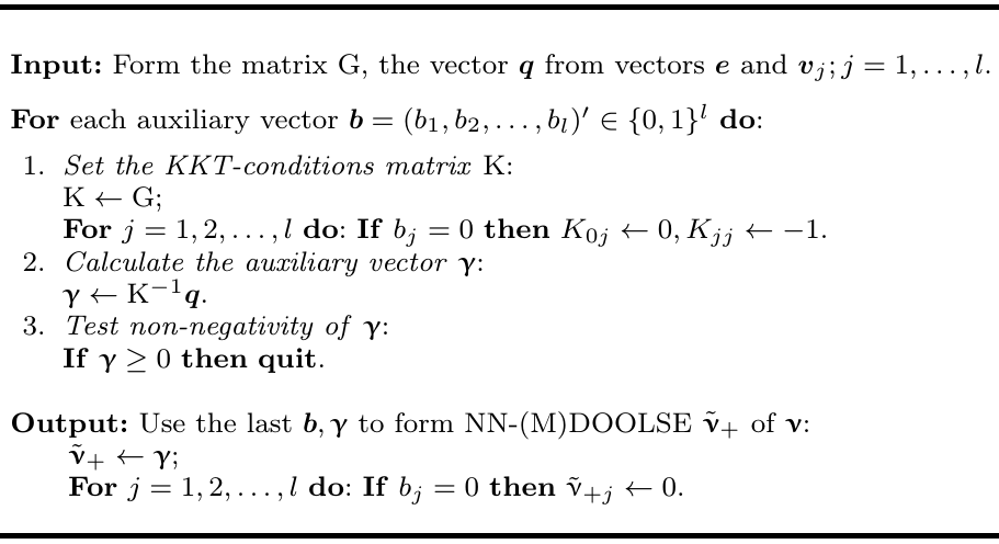
"## KKT algorithm\n",
"using the the KKT algorithm (tab.3, _Hancova et al 2019_) \n",
" \n",
"\n",
"$~$\n",
">$\n",
"\\qquad \\mathbf{q} = \n",
"\\left(\\begin{array}{c}\n",
"\\mathbf{e}' \\mathbf{e}\\\\\n",
"(\\mathbf{e}' \\mathbf{v}_{1})^2 \\\\\n",
"\\vdots \\\\\n",
"(\\mathbf{e}' \\mathbf{v}_{l})^2\n",
"\\end{array}\\right)\n",
"$\n",
">\n",
"> $\\qquad\\mathrm{G} = \\left(\\begin{array}{ccccc}\n",
"\\small\n",
"n^* & ||\\mathbf{v}_{1}||^2 & ||\\mathbf{v}_{2}||^2 & \\ldots & ||\\mathbf{v}_{l}||^2 \\\\\n",
"||\\mathbf{v}_{1}||^2 & ||\\mathbf{v}_{1}||^4 & 0 & \\ldots & 0 \\\\\n",
"||\\mathbf{v}_{2}||^2 & 0 & ||\\mathbf{v}_{2}||^4 & \\ldots & 0 \\\\\n",
"\\vdots & \\vdots & \\vdots & \\ldots & \\vdots \\\\\n",
"||\\mathbf{v}_{l}||^2 & 0 & 0 & \\ldots & ||\\mathbf{v}_{l}||^4\n",
"\\end{array}\\right)\n",
"$"
]
},
{
"cell_type": "code",
"execution_count": 13,
"metadata": {
"ExecuteTime": {
"end_time": "2019-05-19T17:18:30.773000Z",
"start_time": "2019-05-19T17:18:25.636Z"
}
},
"outputs": [],
"source": [
"NNMDOOLSE_kkt <- function(X, F, V, method = \"NNDOOLSE\") {\n",
" n_star <- length(X)\n",
" k <- ncol(F)\n",
" l <- ncol(V)\n",
" if(method == \"NNMDOOLSE\") {\n",
" n_star <- n_star - k\n",
" }\n",
" \n",
" MF <- makeM_F(F)\n",
" u <- diag(t(V) %*% V)\n",
" G <- rbind(c(n_star,u),cbind(u, diag(u^2)))\n",
" b_comb <- expand.grid(rep(list(0:1), l))\n",
" \n",
" eps <- c(MF %*% X)\n",
" q <- c(eps %*% eps, (eps %*% V)^2)\n",
" K <- G\n",
" s <- vector()\n",
" \n",
" for(i in 1:nrow(b_comb)) {\n",
" K_inv <- matrix()\n",
" b <- as.vector(unlist(b_comb[i,]))\n",
" for(j in 1:length(b)) {\n",
" if(b[j] == 0) {\n",
" K[1,j+1] <- 0\n",
" K[j+1,j+1] <- -1\n",
" }\n",
" K_inv <- solve(K)\n",
" }\n",
" beta <- c(K_inv %*% q)\n",
" if(all(beta >= 0)) {\n",
" s <- beta[1]\n",
" for(m in 1:l) {\n",
" if(b[m] == 0) {\n",
" s <- c(s, 0)\n",
" } else {\n",
" s <- c(s, beta[m+1])\n",
" }\n",
" }\n",
" break\n",
" } else {\n",
" K <- G\n",
" }\n",
" }\n",
" return(list(\"estimates\" = s, \"b\" = b))\n",
"}"
]
},
{
"cell_type": "code",
"execution_count": 14,
"metadata": {
"ExecuteTime": {
"end_time": "2019-05-19T17:18:30.853000Z",
"start_time": "2019-05-19T17:18:25.639Z"
}
},
"outputs": [
{
"name": "stdout",
"output_type": "stream",
"text": [
"[1] 0.929088 2.888293 1.684435 0.294511 1.786055\n",
"[1] 3.914013\n",
"[1] 1 1 1 1\n"
]
}
],
"source": [
"NN_DOOLSE <- NNMDOOLSE_kkt(x, F, V)\n",
"print(NN_DOOLSE$estimates)\n",
"print(norm_vec(NN_DOOLSE$estimates))\n",
"print(NN_DOOLSE$b)"
]
},
{
"cell_type": "markdown",
"metadata": {},
"source": [
"## CVXR\n",
"\n",
"nonnegative DOOLSE as a convex optimization problem\n",
"\n",
">$\n",
"\\begin{array}{ll} \n",
"\\textit{minimize} & f_0(\\boldsymbol{\\nu})=||\\mathbf{e}\\mathbf{e}'-\\Sigma_\\boldsymbol{\\nu}||^2 \\\\[6pt]\n",
"\\textit{subject to} & \\boldsymbol{\\nu} = \\left(\\nu_0, \\ldots, \\nu_l\\right)'\\in [0, \\infty)^{l+1} \n",
"\\end{array}\n",
"$"
]
},
{
"cell_type": "code",
"execution_count": 15,
"metadata": {
"ExecuteTime": {
"end_time": "2019-05-19T17:18:30.885000Z",
"start_time": "2019-05-19T17:18:25.642Z"
},
"scrolled": true
},
"outputs": [],
"source": [
"NNDOOLSE_CVXR <- function(X, F, V) {\n",
" n <- length(X)\n",
" k <- ncol(F)\n",
" l <- ncol(V)\n",
"\n",
" # GF <- t(F) %*% F\n",
" # InvGF <- solve(GF)\n",
" I <- diag(n)\n",
" # PF <- F %*% InvGF %*% t(F)\n",
" #MF <- I - PF\n",
" MF <- makeM_F(F)\n",
" MFV <- MF %*% V\n",
"\n",
" SX <- MF %*% X %*% t(X) %*% MF\n",
" s <- Variable(l+1)\n",
" p_obj <- Minimize(sum_squares(SX - (s[1] %*% I) - (V %*% diag(s[2:(l+1)]) %*% t(V))))\n",
" constr <- list(s >= 0)\n",
" prob <- Problem(p_obj, constr)\n",
"\n",
" sol <- solve(prob)\n",
"\n",
" return(as.vector(sol$getValue(s)))\n",
"}"
]
},
{
"cell_type": "code",
"execution_count": 16,
"metadata": {
"ExecuteTime": {
"end_time": "2019-05-19T17:18:32.182000Z",
"start_time": "2019-05-19T17:18:25.644Z"
}
},
"outputs": [
{
"name": "stdout",
"output_type": "stream",
"text": [
"[1] 0.9289981 2.8882994 1.6844382 0.2944570 1.7860596\n",
"[1] 3.913995\n"
]
}
],
"source": [
"NN_DOOLSEcvxr <- NNDOOLSE_CVXR(x, F, V)\n",
"print(NN_DOOLSEcvxr)\n",
"print(norm_vec(NN_DOOLSEcvxr))"
]
},
{
"cell_type": "markdown",
"metadata": {},
"source": [
"## CVXR\n",
"\n",
"using equivalent (RE)MLE convex problem (proposition 5, _Hancova et al 2019_)\n",
"\n",
"\n",
">$\n",
"\\begin{array}{ll} \n",
"\\textit{minimize} & \\quad f_0(\\mathbf{d})=-(n^*\\!-l)\\ln d_0 - \\displaystyle\\sum\\limits_{j=1}^{l} \n",
"\t\t\\ln(d_0-d_j||\\mathbf{v}_j||^2+d_0\\mathbf{e}'\\mathbf{e}-\\mathbf{e}'\\mathrm{V}\\,\\mathrm{diag}\\{d_j\\}\\mathrm{V}'\\mathbf{e} \\\\[6pt]\n",
"\\textit{subject to} & \\quad d_0 > \\max\\{d_j||\\mathbf{v}_j||^2, j = 1, \\ldots, l\\} \\\\\n",
" & \\quad d_j \\geq 0, j=1,\\ldots l \\\\\n",
" & \\\\\n",
"& \\quad\\text{for MLE: } n^* = n, \\text{ for REMLE: } n^* = n-k \\\\\n",
"\\textit{back transformation:} & \\quad \\nu_0 = \\dfrac{1}{d_0}, \\nu_j = \\dfrac{d_j}{d_0\\left(d_0 -d_j||\\mathbf{v}_j||^2\\right)}\n",
"\\end{array}\n",
"$"
]
},
{
"cell_type": "code",
"execution_count": 17,
"metadata": {
"ExecuteTime": {
"end_time": "2019-05-19T17:18:32.227000Z",
"start_time": "2019-05-19T17:18:25.647Z"
}
},
"outputs": [],
"source": [
"MLE_CVXR <- function(X, F, V){\n",
"\n",
" n <- length(X)\n",
" l <- ncol(V)\n",
"\n",
" MF <- makeM_F(F)\n",
" GV <- t(V) %*% V\n",
" p <- n - l\n",
"\n",
" e <- as.vector(MF %*% X)\n",
" ee <- as.numeric(t(e) %*% e)\n",
" eV <- t(e) %*% V\n",
" Ve <- t(V) %*% e\n",
" d <- Variable(l+1)\n",
" logdetS <- p * log(d[1]) + sum(log(d[1] - GV %*% d[2:(l+1)]))\n",
" obj <- Maximize(logdetS - ((d[1] * ee) - (eV %*% diag(d[2:(l+1)]) %*% Ve)))\n",
" constr <- list(d[2:(l+1)] >= 0, d[1] >= max_entries(GV %*% d[2:(l+1)]))\n",
" p_MLE <- Problem(obj, constr)\n",
"\n",
" sol <- solve(p_MLE)\n",
"\n",
" s <- 1 / sol$getValue(d)[1]\n",
" sj <- vector()\n",
" for(j in 2:(l+1)) {\n",
" sj <- c(sj, sol$getValue(d)[j]/(sol$getValue(d)[1] * (sol$getValue(d)[1] - sol$getValue(d)[j] * GV[j-1,j-1])))\n",
" }\n",
" result <- c(s, sj)\n",
"\n",
" return(as.vector(result))\n",
"\n",
"}"
]
},
{
"cell_type": "code",
"execution_count": 18,
"metadata": {
"ExecuteTime": {
"end_time": "2019-05-19T17:18:36.237000Z",
"start_time": "2019-05-19T17:18:25.650Z"
}
},
"outputs": [
{
"name": "stdout",
"output_type": "stream",
"text": [
"[1] 0.929088 2.888294 1.684435 0.294511 1.786056\n",
"[1] 3.914013\n"
]
}
],
"source": [
"MLEcvxr <- MLE_CVXR(x, F, V)\n",
"print(MLEcvxr)\n",
"print(norm_vec(MLEcvxr))"
]
},
{
"cell_type": "markdown",
"metadata": {},
"source": [
"## $\\boldsymbol{2^{nd}}$ stage of EBLUP-NE"
]
},
{
"cell_type": "code",
"execution_count": 19,
"metadata": {
"ExecuteTime": {
"end_time": "2019-05-19T17:18:36.274000Z",
"start_time": "2019-05-19T17:18:25.652Z"
}
},
"outputs": [
{
"name": "stdout",
"output_type": "stream",
"text": [
"[1] 1.0000000 0.9484689 0.9140421 0.6270020 0.9186301\n"
]
}
],
"source": [
"# numerical results\n",
"print(rho2(NN_DOOLSE$estimates))"
]
},
{
"cell_type": "code",
"execution_count": 20,
"metadata": {
"ExecuteTime": {
"end_time": "2019-05-19T17:18:36.318000Z",
"start_time": "2019-05-19T17:18:25.656Z"
}
},
"outputs": [
{
"name": "stdout",
"output_type": "stream",
"text": [
"[1] 1.093045 2.812891 1.610413 0.233204 1.711848\n",
"[1] 3.832146\n"
]
}
],
"source": [
"print(EBLUPNE(NN_DOOLSE$estimates)) \n",
"print(norm_vec(EBLUPNE(NN_DOOLSE$estimates)))"
]
},
{
"cell_type": "markdown",
"metadata": {},
"source": [
"***\n",
"\n",
"# NN-MDOOLSE or REMLE\n",
"using the KKT algorithm (tab.3, _Hancova et al 2019_)\n",
"\n",
"## $\\boldsymbol{1^{st}}$ stage of EBLUP-NE "
]
},
{
"cell_type": "markdown",
"metadata": {},
"source": [
"## KKT algorithm"
]
},
{
"cell_type": "code",
"execution_count": 21,
"metadata": {
"ExecuteTime": {
"end_time": "2019-05-19T17:18:36.355000Z",
"start_time": "2019-05-19T17:18:25.659Z"
}
},
"outputs": [],
"source": [
"NN_MDOOLSE <- NNMDOOLSE_kkt(x, F, V, method = \"NNMDOOLSE\")"
]
},
{
"cell_type": "code",
"execution_count": 22,
"metadata": {
"ExecuteTime": {
"end_time": "2019-05-19T17:18:36.400000Z",
"start_time": "2019-05-19T17:18:25.662Z"
}
},
"outputs": [
{
"name": "stdout",
"output_type": "stream",
"text": [
"[1] 1.0930447 2.8746303 1.6707717 0.2808479 1.7723924\n",
"[1] 3.933189\n",
"[1] 1 1 1 1\n"
]
}
],
"source": [
"print(NN_MDOOLSE$estimates)\n",
"print(norm_vec(NN_MDOOLSE$estimates))\n",
"print(NN_MDOOLSE$b)"
]
},
{
"cell_type": "markdown",
"metadata": {},
"source": [
"## CVXR\n",
"\n",
"nonnegative DOOLSE as a convex optimization problem\n",
"\n",
">$\n",
"\\begin{array}{ll} \n",
"\\textit{minimize} & f_0(\\boldsymbol{\\nu})=||\\mathbf{e}\\mathbf{e}'-\\mathrm{M_F}\\Sigma_\\boldsymbol{\\nu}\\mathrm{M_F}||^2 \\\\[6pt]\n",
"\\textit{subject to} & \\boldsymbol{\\nu} = \\left(\\nu_0, \\ldots, \\nu_l\\right)'\\in [0, \\infty)^{l+1} \n",
"\\end{array}\n",
"$"
]
},
{
"cell_type": "code",
"execution_count": 23,
"metadata": {
"ExecuteTime": {
"end_time": "2019-05-19T17:18:36.432000Z",
"start_time": "2019-05-19T17:18:25.665Z"
},
"scrolled": true
},
"outputs": [],
"source": [
"NNMDOOLSE_CVXR <- function(X, F, V) {\n",
" n <- length(X)\n",
" k <- ncol(F)\n",
" l <- ncol(V)\n",
"\n",
" # GF <- t(F) %*% F\n",
" # InvGF <- solve(GF)\n",
" I <- diag(n)\n",
" # PF <- F %*% InvGF %*% t(F)\n",
" #MF <- I - PF\n",
" MF <- makeM_F(F)\n",
" MFV <- MF %*% V\n",
"\n",
" SX <- MF %*% X %*% t(X) %*% MF\n",
" s <- Variable(l+1)\n",
" p_obj <- Minimize(sum_squares(SX - (s[1] %*% MF) - (MFV %*% diag(s[2:(l+1)]) %*% t(MFV))))\n",
" constr <- list(s >= 0)\n",
" prob <- Problem(p_obj, constr)\n",
"\n",
" sol <- solve(prob)\n",
"\n",
" return(as.vector(sol$getValue(s)))\n",
"}"
]
},
{
"cell_type": "code",
"execution_count": 24,
"metadata": {
"ExecuteTime": {
"end_time": "2019-05-19T17:18:37.630000Z",
"start_time": "2019-05-19T17:18:25.667Z"
}
},
"outputs": [
{
"name": "stdout",
"output_type": "stream",
"text": [
"[1] 1.0930430 2.8746304 1.6707717 0.2808461 1.7723924\n",
"[1] 3.933188\n"
]
}
],
"source": [
"NN_MDOOLSEcvxr <- NNMDOOLSE_CVXR(x, F, V)\n",
"print(NN_MDOOLSEcvxr)\n",
"print(norm_vec(NN_MDOOLSEcvxr))"
]
},
{
"cell_type": "markdown",
"metadata": {},
"source": [
"## CVXR\n",
"\n",
"using equivalent (RE)MLE convex problem (proposition 5, _Hancova et al 2019_)\n",
"\n",
"\n",
">$\n",
"\\begin{array}{ll} \n",
"\\textit{minimize} & \\quad f_0(\\mathbf{d})=-(n^*\\!-l)\\ln d_0 - \\displaystyle\\sum\\limits_{j=1}^{l} \n",
"\t\t\\ln(d_0-d_j||\\mathbf{v}_j||^2+d_0\\mathbf{e}'\\mathbf{e}-\\mathbf{e}'\\mathrm{V}\\,\\mathrm{diag}\\{d_j\\}\\mathrm{V}'\\mathbf{e} \\\\[6pt]\n",
"\\textit{subject to} & \\quad d_0 > \\max\\{d_j||\\mathbf{v}_j||^2, j = 1, \\ldots, l\\} \\\\\n",
" & \\quad d_j \\geq 0, j=1,\\ldots l \\\\\n",
" & \\\\\n",
"& \\quad\\text{for MLE: } n^* = n, \\text{ for REMLE: } n^* = n-k \\\\\n",
"\\textit{back transformation:} & \\quad \\nu_0 = \\dfrac{1}{d_0}, \\nu_j = \\dfrac{d_j}{d_0\\left(d_0 -d_j||\\mathbf{v}_j||^2\\right)}\n",
"\\end{array}\n",
"$"
]
},
{
"cell_type": "code",
"execution_count": 25,
"metadata": {
"ExecuteTime": {
"end_time": "2019-05-19T17:18:37.663000Z",
"start_time": "2019-05-19T17:18:25.669Z"
}
},
"outputs": [],
"source": [
"REMLE_CVXR <- function(X, F, V){\n",
"\n",
" n <- length(X)\n",
" k <- ncol(F)\n",
" l <- ncol(V)\n",
"\n",
" MF <- makeM_F(F)\n",
" GV <- t(V) %*% V\n",
" p <- n - l - k\n",
"\n",
" e <- as.vector(MF %*% X)\n",
" ee <- as.numeric(t(e) %*% e)\n",
" eV <- t(e) %*% V\n",
" Ve <- t(V) %*% e\n",
" d <- Variable(l+1)\n",
" logdetS <- p * log(d[1]) + sum(log(d[1] - GV %*% d[2:(l+1)]))\n",
" obj <- Maximize(logdetS - ((d[1] * ee) - (eV %*% diag(d[2:(l+1)]) %*% Ve)))\n",
" constr <- list(d[2:(l+1)] >= 0, d[1] >= max_entries(GV %*% d[2:(l+1)]))\n",
" p_remle <- Problem(obj, constr)\n",
"\n",
" sol <- solve(p_remle)\n",
"\n",
" s <- 1 / sol$getValue(d)[1]\n",
" sj <- vector()\n",
" for(j in 2:(l+1)) {\n",
" sj <- c(sj, sol$getValue(d)[j]/(sol$getValue(d)[1] * (sol$getValue(d)[1] - sol$getValue(d)[j] * GV[j-1,j-1])))\n",
" }\n",
"\n",
" result <- c(s, sj)\n",
"\n",
" return(as.vector(result))\n",
"}"
]
},
{
"cell_type": "code",
"execution_count": 26,
"metadata": {
"ExecuteTime": {
"end_time": "2019-05-19T17:18:41.708000Z",
"start_time": "2019-05-19T17:18:25.672Z"
}
},
"outputs": [
{
"name": "stdout",
"output_type": "stream",
"text": [
"[1] 1.0930447 2.8746311 1.6707719 0.2808479 1.7723927\n",
"[1] 3.93319\n"
]
}
],
"source": [
"REMLEcvxr <- REMLE_CVXR(x, F, V)\n",
"print(REMLEcvxr)\n",
"print(norm_vec(REMLEcvxr))"
]
},
{
"cell_type": "markdown",
"metadata": {},
"source": [
"## $\\boldsymbol{2^{nd}}$ stage of EBLUP-NE"
]
},
{
"cell_type": "code",
"execution_count": 27,
"metadata": {
"ExecuteTime": {
"end_time": "2019-05-19T17:18:41.741000Z",
"start_time": "2019-05-19T17:18:25.674Z"
}
},
"outputs": [
{
"name": "stdout",
"output_type": "stream",
"text": [
"[1] 1.0000000 0.9395166 0.8992740 0.5701753 0.9046291\n"
]
}
],
"source": [
"# numerical results\n",
"print(rho2(NN_MDOOLSE$estimates))"
]
},
{
"cell_type": "code",
"execution_count": 28,
"metadata": {
"ExecuteTime": {
"end_time": "2019-05-19T17:18:41.777000Z",
"start_time": "2019-05-19T17:18:25.676Z"
}
},
"outputs": [
{
"name": "stdout",
"output_type": "stream",
"text": [
"[1] 1.0930447 2.7863408 1.5843938 0.2120681 1.6857577\n",
"[1] 3.788865\n"
]
}
],
"source": [
"print(EBLUPNE(NN_MDOOLSE$estimates)) \n",
"print(norm_vec(EBLUPNE(NN_MDOOLSE$estimates)))"
]
},
{
"cell_type": "markdown",
"metadata": {},
"source": [
"***\n",
"\n",
"# References \n",
"This notebook belongs to suplementary materials of the paper submitted to Statistical Papers and available at .\n",
"\n",
"* Hančová, M., Vozáriková, G., Gajdoš, A., Hanč, J. (2019). [Estimating variance components in time series\n",
"\tlinear regression models using empirical BLUPs and convex optimization](https://arxiv.org/abs/1905.07771), https://arxiv.org/, 2019.\n",
"\n",
"### Abstract of the paper\n",
"\n",
"We propose a two-stage estimation method of variance components in time series models known as FDSLRMs, whose observations can be described by a linear mixed model (LMM). We based estimating variances, fundamental quantities in a time series forecasting approach called kriging, on the empirical (plug-in) best linear unbiased predictions of unobservable random components in FDSLRM. \n",
"\n",
"The method, providing invariant non-negative quadratic estimators, can be used for any absolutely continuous probability distribution of time series data. As a result of applying the convex optimization and the LMM methodology, we resolved two problems $-$ theoretical existence and equivalence between least squares estimators, non-negative (M)DOOLSE, and maximum likelihood estimators, (RE)MLE, as possible starting points of our method and a \n",
"practical lack of computational implementation for FDSLRM. As for computing (RE)MLE in the case of $ n $ observed time series values, we also discovered a new algorithm of order $\\mathcal{O}(n)$, which at the default precision is $10^7$ times more accurate and $n^2$ times faster than the best current Python(or R)-based computational packages, namely CVXPY, CVXR, nlme, sommer and mixed. \n",
"\n",
"We illustrate our results on three real data sets $-$ electricity consumption, tourism and cyber security $-$ which are easily available, reproducible, sharable and modifiable in the form of interactive Jupyter notebooks."
]
},
{
"cell_type": "markdown",
"metadata": {},
"source": [
"* Štulajter, F., Witkovský, V. (2004). [Estimation of Variances in Orthogonal Finite\n",
"Discrete Spectrum Linear Regression Models](https://link.springer.com/article/10.1007/s001840300299). _Metrika_, 2004, Vol. 60, No. 2, pp. 105–118"
]
},
{
"cell_type": "markdown",
"metadata": {},
"source": [
"| [Table of Contents](#table_of_contents) | [Data and model](#data_and_model) | [Natural estimators](#natural_estimators) | [NN-DOOLSE, MLE](#doolse) | [NN-MDOOLSE, REMLE](#mdoolse) | [References](#references) |"
]
}
],
"metadata": {
"kernelspec": {
"display_name": "R",
"language": "R",
"name": "ir"
},
"language_info": {
"codemirror_mode": "r",
"file_extension": ".r",
"mimetype": "text/x-r-source",
"name": "R",
"pygments_lexer": "r",
"version": "3.5.1"
},
"varInspector": {
"cols": {
"lenName": 16,
"lenType": 16,
"lenVar": 40
},
"kernels_config": {
"python": {
"delete_cmd_postfix": "",
"delete_cmd_prefix": "del ",
"library": "var_list.py",
"varRefreshCmd": "print(var_dic_list())"
},
"r": {
"delete_cmd_postfix": ") ",
"delete_cmd_prefix": "rm(",
"library": "var_list.r",
"varRefreshCmd": "cat(var_dic_list()) "
}
},
"types_to_exclude": [
"module",
"function",
"builtin_function_or_method",
"instance",
"_Feature"
],
"window_display": false
}
},
"nbformat": 4,
"nbformat_minor": 1
}
\n",
"\n",
"$~$\n",
">$\n",
"\\qquad \\mathbf{q} = \n",
"\\left(\\begin{array}{c}\n",
"\\mathbf{e}' \\mathbf{e}\\\\\n",
"(\\mathbf{e}' \\mathbf{v}_{1})^2 \\\\\n",
"\\vdots \\\\\n",
"(\\mathbf{e}' \\mathbf{v}_{l})^2\n",
"\\end{array}\\right)\n",
"$\n",
">\n",
"> $\\qquad\\mathrm{G} = \\left(\\begin{array}{ccccc}\n",
"\\small\n",
"n^* & ||\\mathbf{v}_{1}||^2 & ||\\mathbf{v}_{2}||^2 & \\ldots & ||\\mathbf{v}_{l}||^2 \\\\\n",
"||\\mathbf{v}_{1}||^2 & ||\\mathbf{v}_{1}||^4 & 0 & \\ldots & 0 \\\\\n",
"||\\mathbf{v}_{2}||^2 & 0 & ||\\mathbf{v}_{2}||^4 & \\ldots & 0 \\\\\n",
"\\vdots & \\vdots & \\vdots & \\ldots & \\vdots \\\\\n",
"||\\mathbf{v}_{l}||^2 & 0 & 0 & \\ldots & ||\\mathbf{v}_{l}||^4\n",
"\\end{array}\\right)\n",
"$"
]
},
{
"cell_type": "code",
"execution_count": 13,
"metadata": {
"ExecuteTime": {
"end_time": "2019-05-19T17:18:30.773000Z",
"start_time": "2019-05-19T17:18:25.636Z"
}
},
"outputs": [],
"source": [
"NNMDOOLSE_kkt <- function(X, F, V, method = \"NNDOOLSE\") {\n",
" n_star <- length(X)\n",
" k <- ncol(F)\n",
" l <- ncol(V)\n",
" if(method == \"NNMDOOLSE\") {\n",
" n_star <- n_star - k\n",
" }\n",
" \n",
" MF <- makeM_F(F)\n",
" u <- diag(t(V) %*% V)\n",
" G <- rbind(c(n_star,u),cbind(u, diag(u^2)))\n",
" b_comb <- expand.grid(rep(list(0:1), l))\n",
" \n",
" eps <- c(MF %*% X)\n",
" q <- c(eps %*% eps, (eps %*% V)^2)\n",
" K <- G\n",
" s <- vector()\n",
" \n",
" for(i in 1:nrow(b_comb)) {\n",
" K_inv <- matrix()\n",
" b <- as.vector(unlist(b_comb[i,]))\n",
" for(j in 1:length(b)) {\n",
" if(b[j] == 0) {\n",
" K[1,j+1] <- 0\n",
" K[j+1,j+1] <- -1\n",
" }\n",
" K_inv <- solve(K)\n",
" }\n",
" beta <- c(K_inv %*% q)\n",
" if(all(beta >= 0)) {\n",
" s <- beta[1]\n",
" for(m in 1:l) {\n",
" if(b[m] == 0) {\n",
" s <- c(s, 0)\n",
" } else {\n",
" s <- c(s, beta[m+1])\n",
" }\n",
" }\n",
" break\n",
" } else {\n",
" K <- G\n",
" }\n",
" }\n",
" return(list(\"estimates\" = s, \"b\" = b))\n",
"}"
]
},
{
"cell_type": "code",
"execution_count": 14,
"metadata": {
"ExecuteTime": {
"end_time": "2019-05-19T17:18:30.853000Z",
"start_time": "2019-05-19T17:18:25.639Z"
}
},
"outputs": [
{
"name": "stdout",
"output_type": "stream",
"text": [
"[1] 0.929088 2.888293 1.684435 0.294511 1.786055\n",
"[1] 3.914013\n",
"[1] 1 1 1 1\n"
]
}
],
"source": [
"NN_DOOLSE <- NNMDOOLSE_kkt(x, F, V)\n",
"print(NN_DOOLSE$estimates)\n",
"print(norm_vec(NN_DOOLSE$estimates))\n",
"print(NN_DOOLSE$b)"
]
},
{
"cell_type": "markdown",
"metadata": {},
"source": [
"## CVXR\n",
"\n",
"nonnegative DOOLSE as a convex optimization problem\n",
"\n",
">$\n",
"\\begin{array}{ll} \n",
"\\textit{minimize} & f_0(\\boldsymbol{\\nu})=||\\mathbf{e}\\mathbf{e}'-\\Sigma_\\boldsymbol{\\nu}||^2 \\\\[6pt]\n",
"\\textit{subject to} & \\boldsymbol{\\nu} = \\left(\\nu_0, \\ldots, \\nu_l\\right)'\\in [0, \\infty)^{l+1} \n",
"\\end{array}\n",
"$"
]
},
{
"cell_type": "code",
"execution_count": 15,
"metadata": {
"ExecuteTime": {
"end_time": "2019-05-19T17:18:30.885000Z",
"start_time": "2019-05-19T17:18:25.642Z"
},
"scrolled": true
},
"outputs": [],
"source": [
"NNDOOLSE_CVXR <- function(X, F, V) {\n",
" n <- length(X)\n",
" k <- ncol(F)\n",
" l <- ncol(V)\n",
"\n",
" # GF <- t(F) %*% F\n",
" # InvGF <- solve(GF)\n",
" I <- diag(n)\n",
" # PF <- F %*% InvGF %*% t(F)\n",
" #MF <- I - PF\n",
" MF <- makeM_F(F)\n",
" MFV <- MF %*% V\n",
"\n",
" SX <- MF %*% X %*% t(X) %*% MF\n",
" s <- Variable(l+1)\n",
" p_obj <- Minimize(sum_squares(SX - (s[1] %*% I) - (V %*% diag(s[2:(l+1)]) %*% t(V))))\n",
" constr <- list(s >= 0)\n",
" prob <- Problem(p_obj, constr)\n",
"\n",
" sol <- solve(prob)\n",
"\n",
" return(as.vector(sol$getValue(s)))\n",
"}"
]
},
{
"cell_type": "code",
"execution_count": 16,
"metadata": {
"ExecuteTime": {
"end_time": "2019-05-19T17:18:32.182000Z",
"start_time": "2019-05-19T17:18:25.644Z"
}
},
"outputs": [
{
"name": "stdout",
"output_type": "stream",
"text": [
"[1] 0.9289981 2.8882994 1.6844382 0.2944570 1.7860596\n",
"[1] 3.913995\n"
]
}
],
"source": [
"NN_DOOLSEcvxr <- NNDOOLSE_CVXR(x, F, V)\n",
"print(NN_DOOLSEcvxr)\n",
"print(norm_vec(NN_DOOLSEcvxr))"
]
},
{
"cell_type": "markdown",
"metadata": {},
"source": [
"## CVXR\n",
"\n",
"using equivalent (RE)MLE convex problem (proposition 5, _Hancova et al 2019_)\n",
"\n",
"\n",
">$\n",
"\\begin{array}{ll} \n",
"\\textit{minimize} & \\quad f_0(\\mathbf{d})=-(n^*\\!-l)\\ln d_0 - \\displaystyle\\sum\\limits_{j=1}^{l} \n",
"\t\t\\ln(d_0-d_j||\\mathbf{v}_j||^2+d_0\\mathbf{e}'\\mathbf{e}-\\mathbf{e}'\\mathrm{V}\\,\\mathrm{diag}\\{d_j\\}\\mathrm{V}'\\mathbf{e} \\\\[6pt]\n",
"\\textit{subject to} & \\quad d_0 > \\max\\{d_j||\\mathbf{v}_j||^2, j = 1, \\ldots, l\\} \\\\\n",
" & \\quad d_j \\geq 0, j=1,\\ldots l \\\\\n",
" & \\\\\n",
"& \\quad\\text{for MLE: } n^* = n, \\text{ for REMLE: } n^* = n-k \\\\\n",
"\\textit{back transformation:} & \\quad \\nu_0 = \\dfrac{1}{d_0}, \\nu_j = \\dfrac{d_j}{d_0\\left(d_0 -d_j||\\mathbf{v}_j||^2\\right)}\n",
"\\end{array}\n",
"$"
]
},
{
"cell_type": "code",
"execution_count": 17,
"metadata": {
"ExecuteTime": {
"end_time": "2019-05-19T17:18:32.227000Z",
"start_time": "2019-05-19T17:18:25.647Z"
}
},
"outputs": [],
"source": [
"MLE_CVXR <- function(X, F, V){\n",
"\n",
" n <- length(X)\n",
" l <- ncol(V)\n",
"\n",
" MF <- makeM_F(F)\n",
" GV <- t(V) %*% V\n",
" p <- n - l\n",
"\n",
" e <- as.vector(MF %*% X)\n",
" ee <- as.numeric(t(e) %*% e)\n",
" eV <- t(e) %*% V\n",
" Ve <- t(V) %*% e\n",
" d <- Variable(l+1)\n",
" logdetS <- p * log(d[1]) + sum(log(d[1] - GV %*% d[2:(l+1)]))\n",
" obj <- Maximize(logdetS - ((d[1] * ee) - (eV %*% diag(d[2:(l+1)]) %*% Ve)))\n",
" constr <- list(d[2:(l+1)] >= 0, d[1] >= max_entries(GV %*% d[2:(l+1)]))\n",
" p_MLE <- Problem(obj, constr)\n",
"\n",
" sol <- solve(p_MLE)\n",
"\n",
" s <- 1 / sol$getValue(d)[1]\n",
" sj <- vector()\n",
" for(j in 2:(l+1)) {\n",
" sj <- c(sj, sol$getValue(d)[j]/(sol$getValue(d)[1] * (sol$getValue(d)[1] - sol$getValue(d)[j] * GV[j-1,j-1])))\n",
" }\n",
" result <- c(s, sj)\n",
"\n",
" return(as.vector(result))\n",
"\n",
"}"
]
},
{
"cell_type": "code",
"execution_count": 18,
"metadata": {
"ExecuteTime": {
"end_time": "2019-05-19T17:18:36.237000Z",
"start_time": "2019-05-19T17:18:25.650Z"
}
},
"outputs": [
{
"name": "stdout",
"output_type": "stream",
"text": [
"[1] 0.929088 2.888294 1.684435 0.294511 1.786056\n",
"[1] 3.914013\n"
]
}
],
"source": [
"MLEcvxr <- MLE_CVXR(x, F, V)\n",
"print(MLEcvxr)\n",
"print(norm_vec(MLEcvxr))"
]
},
{
"cell_type": "markdown",
"metadata": {},
"source": [
"## $\\boldsymbol{2^{nd}}$ stage of EBLUP-NE"
]
},
{
"cell_type": "code",
"execution_count": 19,
"metadata": {
"ExecuteTime": {
"end_time": "2019-05-19T17:18:36.274000Z",
"start_time": "2019-05-19T17:18:25.652Z"
}
},
"outputs": [
{
"name": "stdout",
"output_type": "stream",
"text": [
"[1] 1.0000000 0.9484689 0.9140421 0.6270020 0.9186301\n"
]
}
],
"source": [
"# numerical results\n",
"print(rho2(NN_DOOLSE$estimates))"
]
},
{
"cell_type": "code",
"execution_count": 20,
"metadata": {
"ExecuteTime": {
"end_time": "2019-05-19T17:18:36.318000Z",
"start_time": "2019-05-19T17:18:25.656Z"
}
},
"outputs": [
{
"name": "stdout",
"output_type": "stream",
"text": [
"[1] 1.093045 2.812891 1.610413 0.233204 1.711848\n",
"[1] 3.832146\n"
]
}
],
"source": [
"print(EBLUPNE(NN_DOOLSE$estimates)) \n",
"print(norm_vec(EBLUPNE(NN_DOOLSE$estimates)))"
]
},
{
"cell_type": "markdown",
"metadata": {},
"source": [
"***\n",
"\n",
"# NN-MDOOLSE or REMLE\n",
"using the KKT algorithm (tab.3, _Hancova et al 2019_)\n",
"\n",
"## $\\boldsymbol{1^{st}}$ stage of EBLUP-NE "
]
},
{
"cell_type": "markdown",
"metadata": {},
"source": [
"## KKT algorithm"
]
},
{
"cell_type": "code",
"execution_count": 21,
"metadata": {
"ExecuteTime": {
"end_time": "2019-05-19T17:18:36.355000Z",
"start_time": "2019-05-19T17:18:25.659Z"
}
},
"outputs": [],
"source": [
"NN_MDOOLSE <- NNMDOOLSE_kkt(x, F, V, method = \"NNMDOOLSE\")"
]
},
{
"cell_type": "code",
"execution_count": 22,
"metadata": {
"ExecuteTime": {
"end_time": "2019-05-19T17:18:36.400000Z",
"start_time": "2019-05-19T17:18:25.662Z"
}
},
"outputs": [
{
"name": "stdout",
"output_type": "stream",
"text": [
"[1] 1.0930447 2.8746303 1.6707717 0.2808479 1.7723924\n",
"[1] 3.933189\n",
"[1] 1 1 1 1\n"
]
}
],
"source": [
"print(NN_MDOOLSE$estimates)\n",
"print(norm_vec(NN_MDOOLSE$estimates))\n",
"print(NN_MDOOLSE$b)"
]
},
{
"cell_type": "markdown",
"metadata": {},
"source": [
"## CVXR\n",
"\n",
"nonnegative DOOLSE as a convex optimization problem\n",
"\n",
">$\n",
"\\begin{array}{ll} \n",
"\\textit{minimize} & f_0(\\boldsymbol{\\nu})=||\\mathbf{e}\\mathbf{e}'-\\mathrm{M_F}\\Sigma_\\boldsymbol{\\nu}\\mathrm{M_F}||^2 \\\\[6pt]\n",
"\\textit{subject to} & \\boldsymbol{\\nu} = \\left(\\nu_0, \\ldots, \\nu_l\\right)'\\in [0, \\infty)^{l+1} \n",
"\\end{array}\n",
"$"
]
},
{
"cell_type": "code",
"execution_count": 23,
"metadata": {
"ExecuteTime": {
"end_time": "2019-05-19T17:18:36.432000Z",
"start_time": "2019-05-19T17:18:25.665Z"
},
"scrolled": true
},
"outputs": [],
"source": [
"NNMDOOLSE_CVXR <- function(X, F, V) {\n",
" n <- length(X)\n",
" k <- ncol(F)\n",
" l <- ncol(V)\n",
"\n",
" # GF <- t(F) %*% F\n",
" # InvGF <- solve(GF)\n",
" I <- diag(n)\n",
" # PF <- F %*% InvGF %*% t(F)\n",
" #MF <- I - PF\n",
" MF <- makeM_F(F)\n",
" MFV <- MF %*% V\n",
"\n",
" SX <- MF %*% X %*% t(X) %*% MF\n",
" s <- Variable(l+1)\n",
" p_obj <- Minimize(sum_squares(SX - (s[1] %*% MF) - (MFV %*% diag(s[2:(l+1)]) %*% t(MFV))))\n",
" constr <- list(s >= 0)\n",
" prob <- Problem(p_obj, constr)\n",
"\n",
" sol <- solve(prob)\n",
"\n",
" return(as.vector(sol$getValue(s)))\n",
"}"
]
},
{
"cell_type": "code",
"execution_count": 24,
"metadata": {
"ExecuteTime": {
"end_time": "2019-05-19T17:18:37.630000Z",
"start_time": "2019-05-19T17:18:25.667Z"
}
},
"outputs": [
{
"name": "stdout",
"output_type": "stream",
"text": [
"[1] 1.0930430 2.8746304 1.6707717 0.2808461 1.7723924\n",
"[1] 3.933188\n"
]
}
],
"source": [
"NN_MDOOLSEcvxr <- NNMDOOLSE_CVXR(x, F, V)\n",
"print(NN_MDOOLSEcvxr)\n",
"print(norm_vec(NN_MDOOLSEcvxr))"
]
},
{
"cell_type": "markdown",
"metadata": {},
"source": [
"## CVXR\n",
"\n",
"using equivalent (RE)MLE convex problem (proposition 5, _Hancova et al 2019_)\n",
"\n",
"\n",
">$\n",
"\\begin{array}{ll} \n",
"\\textit{minimize} & \\quad f_0(\\mathbf{d})=-(n^*\\!-l)\\ln d_0 - \\displaystyle\\sum\\limits_{j=1}^{l} \n",
"\t\t\\ln(d_0-d_j||\\mathbf{v}_j||^2+d_0\\mathbf{e}'\\mathbf{e}-\\mathbf{e}'\\mathrm{V}\\,\\mathrm{diag}\\{d_j\\}\\mathrm{V}'\\mathbf{e} \\\\[6pt]\n",
"\\textit{subject to} & \\quad d_0 > \\max\\{d_j||\\mathbf{v}_j||^2, j = 1, \\ldots, l\\} \\\\\n",
" & \\quad d_j \\geq 0, j=1,\\ldots l \\\\\n",
" & \\\\\n",
"& \\quad\\text{for MLE: } n^* = n, \\text{ for REMLE: } n^* = n-k \\\\\n",
"\\textit{back transformation:} & \\quad \\nu_0 = \\dfrac{1}{d_0}, \\nu_j = \\dfrac{d_j}{d_0\\left(d_0 -d_j||\\mathbf{v}_j||^2\\right)}\n",
"\\end{array}\n",
"$"
]
},
{
"cell_type": "code",
"execution_count": 25,
"metadata": {
"ExecuteTime": {
"end_time": "2019-05-19T17:18:37.663000Z",
"start_time": "2019-05-19T17:18:25.669Z"
}
},
"outputs": [],
"source": [
"REMLE_CVXR <- function(X, F, V){\n",
"\n",
" n <- length(X)\n",
" k <- ncol(F)\n",
" l <- ncol(V)\n",
"\n",
" MF <- makeM_F(F)\n",
" GV <- t(V) %*% V\n",
" p <- n - l - k\n",
"\n",
" e <- as.vector(MF %*% X)\n",
" ee <- as.numeric(t(e) %*% e)\n",
" eV <- t(e) %*% V\n",
" Ve <- t(V) %*% e\n",
" d <- Variable(l+1)\n",
" logdetS <- p * log(d[1]) + sum(log(d[1] - GV %*% d[2:(l+1)]))\n",
" obj <- Maximize(logdetS - ((d[1] * ee) - (eV %*% diag(d[2:(l+1)]) %*% Ve)))\n",
" constr <- list(d[2:(l+1)] >= 0, d[1] >= max_entries(GV %*% d[2:(l+1)]))\n",
" p_remle <- Problem(obj, constr)\n",
"\n",
" sol <- solve(p_remle)\n",
"\n",
" s <- 1 / sol$getValue(d)[1]\n",
" sj <- vector()\n",
" for(j in 2:(l+1)) {\n",
" sj <- c(sj, sol$getValue(d)[j]/(sol$getValue(d)[1] * (sol$getValue(d)[1] - sol$getValue(d)[j] * GV[j-1,j-1])))\n",
" }\n",
"\n",
" result <- c(s, sj)\n",
"\n",
" return(as.vector(result))\n",
"}"
]
},
{
"cell_type": "code",
"execution_count": 26,
"metadata": {
"ExecuteTime": {
"end_time": "2019-05-19T17:18:41.708000Z",
"start_time": "2019-05-19T17:18:25.672Z"
}
},
"outputs": [
{
"name": "stdout",
"output_type": "stream",
"text": [
"[1] 1.0930447 2.8746311 1.6707719 0.2808479 1.7723927\n",
"[1] 3.93319\n"
]
}
],
"source": [
"REMLEcvxr <- REMLE_CVXR(x, F, V)\n",
"print(REMLEcvxr)\n",
"print(norm_vec(REMLEcvxr))"
]
},
{
"cell_type": "markdown",
"metadata": {},
"source": [
"## $\\boldsymbol{2^{nd}}$ stage of EBLUP-NE"
]
},
{
"cell_type": "code",
"execution_count": 27,
"metadata": {
"ExecuteTime": {
"end_time": "2019-05-19T17:18:41.741000Z",
"start_time": "2019-05-19T17:18:25.674Z"
}
},
"outputs": [
{
"name": "stdout",
"output_type": "stream",
"text": [
"[1] 1.0000000 0.9395166 0.8992740 0.5701753 0.9046291\n"
]
}
],
"source": [
"# numerical results\n",
"print(rho2(NN_MDOOLSE$estimates))"
]
},
{
"cell_type": "code",
"execution_count": 28,
"metadata": {
"ExecuteTime": {
"end_time": "2019-05-19T17:18:41.777000Z",
"start_time": "2019-05-19T17:18:25.676Z"
}
},
"outputs": [
{
"name": "stdout",
"output_type": "stream",
"text": [
"[1] 1.0930447 2.7863408 1.5843938 0.2120681 1.6857577\n",
"[1] 3.788865\n"
]
}
],
"source": [
"print(EBLUPNE(NN_MDOOLSE$estimates)) \n",
"print(norm_vec(EBLUPNE(NN_MDOOLSE$estimates)))"
]
},
{
"cell_type": "markdown",
"metadata": {},
"source": [
"***\n",
"\n",
"# References \n",
"This notebook belongs to suplementary materials of the paper submitted to Statistical Papers and available at .\n",
"\n",
"* Hančová, M., Vozáriková, G., Gajdoš, A., Hanč, J. (2019). [Estimating variance components in time series\n",
"\tlinear regression models using empirical BLUPs and convex optimization](https://arxiv.org/abs/1905.07771), https://arxiv.org/, 2019.\n",
"\n",
"### Abstract of the paper\n",
"\n",
"We propose a two-stage estimation method of variance components in time series models known as FDSLRMs, whose observations can be described by a linear mixed model (LMM). We based estimating variances, fundamental quantities in a time series forecasting approach called kriging, on the empirical (plug-in) best linear unbiased predictions of unobservable random components in FDSLRM. \n",
"\n",
"The method, providing invariant non-negative quadratic estimators, can be used for any absolutely continuous probability distribution of time series data. As a result of applying the convex optimization and the LMM methodology, we resolved two problems $-$ theoretical existence and equivalence between least squares estimators, non-negative (M)DOOLSE, and maximum likelihood estimators, (RE)MLE, as possible starting points of our method and a \n",
"practical lack of computational implementation for FDSLRM. As for computing (RE)MLE in the case of $ n $ observed time series values, we also discovered a new algorithm of order $\\mathcal{O}(n)$, which at the default precision is $10^7$ times more accurate and $n^2$ times faster than the best current Python(or R)-based computational packages, namely CVXPY, CVXR, nlme, sommer and mixed. \n",
"\n",
"We illustrate our results on three real data sets $-$ electricity consumption, tourism and cyber security $-$ which are easily available, reproducible, sharable and modifiable in the form of interactive Jupyter notebooks."
]
},
{
"cell_type": "markdown",
"metadata": {},
"source": [
"* Štulajter, F., Witkovský, V. (2004). [Estimation of Variances in Orthogonal Finite\n",
"Discrete Spectrum Linear Regression Models](https://link.springer.com/article/10.1007/s001840300299). _Metrika_, 2004, Vol. 60, No. 2, pp. 105–118"
]
},
{
"cell_type": "markdown",
"metadata": {},
"source": [
"| [Table of Contents](#table_of_contents) | [Data and model](#data_and_model) | [Natural estimators](#natural_estimators) | [NN-DOOLSE, MLE](#doolse) | [NN-MDOOLSE, REMLE](#mdoolse) | [References](#references) |"
]
}
],
"metadata": {
"kernelspec": {
"display_name": "R",
"language": "R",
"name": "ir"
},
"language_info": {
"codemirror_mode": "r",
"file_extension": ".r",
"mimetype": "text/x-r-source",
"name": "R",
"pygments_lexer": "r",
"version": "3.5.1"
},
"varInspector": {
"cols": {
"lenName": 16,
"lenType": 16,
"lenVar": 40
},
"kernels_config": {
"python": {
"delete_cmd_postfix": "",
"delete_cmd_prefix": "del ",
"library": "var_list.py",
"varRefreshCmd": "print(var_dic_list())"
},
"r": {
"delete_cmd_postfix": ") ",
"delete_cmd_prefix": "rm(",
"library": "var_list.r",
"varRefreshCmd": "cat(var_dic_list()) "
}
},
"types_to_exclude": [
"module",
"function",
"builtin_function_or_method",
"instance",
"_Feature"
],
"window_display": false
}
},
"nbformat": 4,
"nbformat_minor": 1
}