{
"cells": [
{
"cell_type": "markdown",
"metadata": {},
"source": [
"| [Table of Contents](#table_of_contents) | [Data and model](#data_and_model) | [Natural estimators](#natural_estimators) | [NN-DOOLSE, MLE](#doolse) | [NN-MDOOLSE, REMLE](#mdoolse) | [References](#references) |"
]
},
{
"cell_type": "markdown",
"metadata": {},
"source": [
"**Authors:** Jozef Hanč, Martina Hančová, Andrej Gajdoš
*[Faculty of Science](https://www.upjs.sk/en/faculty-of-science/?prefferedLang=EN), P. J. Šafárik University in Košice, Slovakia*
emails: [martina.hancova@upjs.sk](mailto:martina.hancova@upjs.sk)\n",
"***\n",
"** EBLUP-NE for electricity consumption 2** "
]
},
{
"cell_type": "markdown",
"metadata": {},
"source": [
" Python-based computational tools - **SageMath** \n",
"\n",
"### Table of Contents \n",
"* [Data and model](#data_and_model) - data and model description of empirical data\n",
"* [Natural estimators](#natural_estimators) - EBLUPNE based on NE\n",
"* [NN-DOOLSE, MLE](#doolse) - EBLUPNE based on nonnegative DOOLSE (same as MLE)\n",
"* [NN-MDOOLSE, REMLE](#mdoolse) - EBLUPNE based on nonnegative MDOOLSE (same as REMLE)\n",
"* [References](#references)\n",
"\n",
"**To get back to the contents, use the Home key.**"
]
},
{
"cell_type": "markdown",
"metadata": {},
"source": [
"## SageMath - precision and functions\n",
"SageMath is a free Python-based mathematics software, an open source alternative to the well-known commercial \n",
"computer algebra systems Mathematica or Maple, which is built on top of SciPy ecosystem, Maxima, R, GAP, FLINT and many others open-source packages; http://www.sagemath.org/"
]
},
{
"cell_type": "code",
"execution_count": 1,
"metadata": {},
"outputs": [],
"source": [
"# arbitrary precision in dps decimal places for numerical results \n",
"dps = 20\n",
"\n",
"# precision in bits, real (floating-point) numbers with given precision \n",
"bits = round((dps+1)*ln(10)/ln(2))\n",
"RRk = RealField(bits)\n",
"\n",
"# simplifying any symbolic matrix, vector\n",
"def simplify_matrix(A): return A.apply_map(lambda item: item.expand())\n",
"\n",
"# converting symbolic matrix, vector to numerical in RRk\n",
"def RRk_matrix(A): return A.apply_map(RRk)\n",
"\n",
"from itertools import product"
]
},
{
"cell_type": "markdown",
"metadata": {},
"source": [
"***\n",
"\n",
"# Data and Model"
]
},
{
"cell_type": "markdown",
"metadata": {},
"source": [
"In this FDSLRM application, we model the econometric time series data set, representing the hours observations of the consumption of the electric energy in some department store. The number of time series observations is $n=24$. The data and model were adapted from _Štulajter & Witkovský, 2004_.\n",
"\n",
"The consumption data can be fitted by the following Gaussian orthogonal FDSLRM:\n",
"\n",
"$ \n",
"\\begin{array}{rl}\n",
"& X(t) & \\! = \\! & \\beta_1+\\beta_2\\cos\\left(\\tfrac{2\\pi t}{24}\\right)+\\beta_3\\sin\\left(\\tfrac{2\\pi t}{24}\\right) +\\\\\n",
"& & & +Y_1\\cos\\left(\\tfrac{2\\pi t\\cdot 2}{24}\\right)+Y_2\\sin\\left(\\tfrac{2\\pi t\\cdot 2}{24}\\right)+\\\\\n",
"& & & +Y_3\\cos\\left(\\tfrac{2\\pi t\\cdot 3}{24}\\right)+Y_4\\sin\\left(\\tfrac{2\\pi t\\cdot 3}{24}\\right)\n",
"+w(t), \\, t\\in \\mathbb{N},\n",
"\\end{array}\n",
"$ \n",
"\n",
"where $\\boldsymbol{\\beta}=(\\beta_1,\\,\\beta_2,\\,\\beta_3)' \\in \\mathbb{R}^3\\,,\\mathbf{Y} = (Y_1, Y_2, Y_3, Y_4)' \\sim \\mathcal{N}_4(\\boldsymbol{0}, \\mathrm{D})\\,, w(t) \\sim \\mathcal{iid}\\, \\mathcal{N} (0, \\sigma_0^2)\\,, \\boldsymbol{\\nu}= (\\sigma_0^2, \\sigma_1^2, \\sigma_2^2, \\sigma_3^2, \\sigma_4^2) \\in \\mathbb{R}_{+}^5.$ "
]
},
{
"cell_type": "code",
"execution_count": 2,
"metadata": {},
"outputs": [
{
"data": {
"text/plain": [
"[403/10 407/10 77/2 379/10 193/5 411/10 226/5 457/10 467/10 93/2 226/5 451/10 229/5 463/10 95/2 97/2 491/10 517/10 253/5 48 447/10 206/5 40 403/10]"
]
},
"execution_count": 2,
"metadata": {},
"output_type": "execute_result"
}
],
"source": [
"# data - time series observation x\n",
"data = [40.3,40.7,38.5,37.9,38.6,41.1,45.2,45.7,46.7,46.5,\n",
" 45.2,45.1,45.8,46.3,47.5,48.5,49.1,51.7,50.6,48.0,\n",
" 44.7,41.2,40.0,40.3]\n",
"\n",
"# observation x as a one-column matrix of rational numbers (infinite precision)\n",
"x = matrix(QQ, data).T\n",
"xc = x.T\n",
"xc"
]
},
{
"cell_type": "code",
"execution_count": 3,
"metadata": {},
"outputs": [],
"source": [
"# model parameters\n",
"n, k, l = 24, 3, 4\n",
"\n",
"# significant frequencies\n",
"om1, om2, om3 = 2*pi/24, 2*pi/12, 2*pi/8\n",
"\n",
"# model design matrices F', F, V',V\n",
"Fc = matrix([[1 for t in range(1,n+1)],\n",
" [cos(om1*t) for t in range(1,n+1)],\n",
" [sin(om1*t) for t in range(1,n+1)]])\n",
"Vc = matrix([[cos(om2*t) for t in range(1,n+1)],\n",
" [sin(om2*t) for t in range(1,n+1)],\n",
" [cos(om3*t) for t in range(1,n+1)],\n",
" [sin(om3*t) for t in range(1,n+1)]])\n",
"F, V = Fc.T, Vc.T\n",
"\n",
"# columns vj of V and their squared norm ||vj||^2\n",
"vv = lambda j: V[:,j-1]\n",
"nv2 = lambda j: (vv(j).T*vv(j)).trace().expand()"
]
},
{
"cell_type": "code",
"execution_count": 4,
"metadata": {},
"outputs": [],
"source": [
"# auxiliary matrices and vectors\n",
"\n",
"# Gram matrices GF, GV\n",
"GF, GV = (Fc*F).expand(), (Vc*V).expand()\n",
"InvGF, InvGV = (GF^(-1)).expand(), (GV^(-1)).expand()\n",
"\n",
"# projectors PF, MF, PV, MV\n",
"In = identity_matrix(n)\n",
"PF = (F*InvGF*Fc).canonicalize_radical().expand()\n",
"PV = (V*InvGV*Vc).canonicalize_radical().expand()\n",
"MF, MV = (In-PF).expand(), (In-PV).expand()\n",
"\n",
"# residuals e, e'\n",
"e = MF*x\n",
"ec = e.T"
]
},
{
"cell_type": "code",
"execution_count": 5,
"metadata": {
"ExecuteTime": {
"end_time": "2019-05-12T14:02:10.103000Z",
"start_time": "2019-05-12T14:02:10.091000Z"
}
},
"outputs": [
{
"data": {
"text/html": [
""
],
"text/plain": [
"[0 0 0 0]\n",
"[0 0 0 0]\n",
"[0 0 0 0]"
]
},
"metadata": {},
"output_type": "display_data"
},
{
"data": {
"text/html": [
""
],
"text/plain": [
"[12 0 0 0]\n",
"[ 0 12 0 0]\n",
"[ 0 0 12 0]\n",
"[ 0 0 0 12]"
]
},
"metadata": {},
"output_type": "display_data"
}
],
"source": [
"# orthogonality condition\n",
"show((Fc*V).expand())\n",
"show(GV)"
]
},
{
"cell_type": "markdown",
"metadata": {},
"source": [
"***\n",
"\n",
"# Natural estimators\n",
"\n",
"## ANALYTICALLY \n",
"using formula (4.1) from _Hancova et al 2019_\n",
"\n",
">$\n",
"\\renewcommand{\\arraystretch}{1.4}\n",
"\\breve{\\boldsymbol{\\nu}}(\\mathbf{e}) =\n",
"\\begin{pmatrix}\n",
"\\tfrac{1}{n-k-l}\\,\\mathbf{e}'\\,\\mathrm{M_V}\\,\\mathbf{e} \\\\\n",
"(\\mathbf{e}'\\mathbf{v}_1)^2/||\\mathbf{v}_1||^4 \\\\\n",
"\\vdots \\\\\n",
"(\\mathbf{e}'\\mathbf{v}_l)^2/||\\mathbf{v}_l||^4\n",
"\\end{pmatrix} \n",
"$\n",
"\n",
"## $\\boldsymbol{1^{st}}$ stage of EBLUP-NE "
]
},
{
"cell_type": "code",
"execution_count": 6,
"metadata": {},
"outputs": [],
"source": [
"# NE according to formula (4.1)\n",
"NE0 = [1/(n-k-l)*(ec*MV*e).trace()]\n",
"NEj = [((ec*vv(j)).trace()/nv2(j))^2 for j in [1..l]] \n",
"NE = vector(NE0+NEj)"
]
},
{
"cell_type": "code",
"execution_count": 7,
"metadata": {},
"outputs": [
{
"data": {
"text/html": [
""
],
"text/plain": [
"[-6569/4080*sqrt(3)*sqrt(2) - 13207/4080*sqrt(3) - 22533/6800*sqrt(2) + 312727/20400]\n",
"[ 6161/7200*sqrt(3) + 5341/3600]\n",
"[ 1/2*sqrt(3) + 43/48]\n",
"[ 21/160*sqrt(2) + 2683/14400]\n",
"[ 4429/7200*sqrt(2) + 4769/4800]"
]
},
"metadata": {},
"output_type": "display_data"
}
],
"source": [
"# final NE\n",
"NEsimp = NE.column().expand()\n",
"show(NEsimp)"
]
},
{
"cell_type": "code",
"execution_count": 8,
"metadata": {},
"outputs": [
{
"data": {
"text/plain": [
"[ 1.0930446920400417197]\n",
"[ 2.9657173646433129174]\n",
"[ 1.7618587371177719801]\n",
"[0.37193497450591316960]\n",
"[ 1.8634794260764497182]"
]
},
"execution_count": 8,
"metadata": {},
"output_type": "execute_result"
}
],
"source": [
"# numerical results with given precision in dps\n",
"NEnum = RRk_matrix(NEsimp)\n",
"NEnum"
]
},
{
"cell_type": "code",
"execution_count": 9,
"metadata": {},
"outputs": [
{
"data": {
"text/plain": [
"4.087207309639791"
]
},
"execution_count": 9,
"metadata": {},
"output_type": "execute_result"
}
],
"source": [
"NEnum.norm()"
]
},
{
"cell_type": "markdown",
"metadata": {},
"source": [
"## $\\boldsymbol{2^{nd}}$ stage of EBLUP-NE\n",
"using formula (3.10) from _Hancova et al 2019_.\n",
">$\n",
"\\mathring{\\nu}_j = \\rho_j^2 \\breve{\\nu}_j; j = 0,1 \\ldots, l\\\\\n",
"\\rho_0 = 1, \\rho_j = \\dfrac{\\hat{\\nu}_j||\\mathbf{v}_j||^2}{\\hat{\\nu}_0+\\hat{\\nu}_j||\\mathbf{v}_j||^2} \n",
"$\n",
">\n",
">where $\\boldsymbol{\\breve{\\nu}}$ are NE, $\\boldsymbol{\\hat{\\nu}}$ are initial estimates for EBLUP-NE"
]
},
{
"cell_type": "code",
"execution_count": 10,
"metadata": {},
"outputs": [],
"source": [
"# EBLUP-NE based on formula (3.9)\n",
"rho2 = lambda est: vector( [1] + [ (est[j]*nv2(j)/(est[0]+est[j]*nv2(j)))^2 for j in [1..l] ])\n",
"EBLUPNE = lambda est: vector( rho2(est).pairwise_product(NE).list() )"
]
},
{
"cell_type": "code",
"execution_count": 11,
"metadata": {
"scrolled": true
},
"outputs": [
{
"data": {
"text/html": [
""
],
"text/plain": [
"[ -6569/4080*sqrt(3)*sqrt(2) - 13207/4080*sqrt(3) - 22533/6800*sqrt(2) + 312727/20400]\n",
"[ -54150532290161/720*sqrt(3)/(10632253712*sqrt(3)*sqrt(2) - 33797716665*sqrt(3) + 19941646650*sqrt(2) - 89032890190) - 703436049059737/5400/(10632253712*sqrt(3)*sqrt(2) - 33797716665*sqrt(3) + 19941646650*sqrt(2) - 89032890190)]\n",
"[ -47305687500*sqrt(3)/(21284644450*sqrt(3)*sqrt(2) - 34428280165*sqrt(3) + 41518418448*sqrt(2) - 154097891078) - 163873295625/2/(21284644450*sqrt(3)*sqrt(2) - 34428280165*sqrt(3) + 41518418448*sqrt(2) - 154097891078)]\n",
"[ -58140346341/160*sqrt(2)/(6284944130*sqrt(3)*sqrt(2) + 14221927480*sqrt(3) + 4135421198*sqrt(2) - 50158949997) - 22200174206443/43200/(6284944130*sqrt(3)*sqrt(2) + 14221927480*sqrt(3) + 4135421198*sqrt(2) - 50158949997)]\n",
"[-39474566680703/288*sqrt(2)/(47480185830*sqrt(3)*sqrt(2) + 84326620280*sqrt(3) - 105286098854*sqrt(2) - 342404267079) - 310322553535051/1600/(47480185830*sqrt(3)*sqrt(2) + 84326620280*sqrt(3) - 105286098854*sqrt(2) - 342404267079)]"
]
},
"metadata": {},
"output_type": "display_data"
}
],
"source": [
"# final EBLUPNE based on NE\n",
"EBLUPNEsimp = EBLUPNE(NE).column().expand()\n",
"show(EBLUPNEsimp)"
]
},
{
"cell_type": "code",
"execution_count": 12,
"metadata": {},
"outputs": [
{
"data": {
"text/plain": [
"[ 1]\n",
"[0.94129166721252861086]\n",
"[0.90410056203431227372]\n",
"[0.64525402743480536407]\n",
"[0.90896740457337881883]"
]
},
"execution_count": 12,
"metadata": {},
"output_type": "execute_result"
}
],
"source": [
"# numerical results\n",
"rho2(NEnum).column()"
]
},
{
"cell_type": "code",
"execution_count": 13,
"metadata": {},
"outputs": [
{
"data": {
"text/plain": [
"[ 1.0930446920400417197]\n",
"[ 2.7916050426462506682]\n",
"[ 1.5928974744532412866]\n",
"[0.23999254024380213000]\n",
"[ 1.6938420573966000382]"
]
},
"execution_count": 13,
"metadata": {},
"output_type": "execute_result"
}
],
"source": [
"EBLUPNEnum = RRk_matrix(EBLUPNEsimp)\n",
"EBLUPNEnum "
]
},
{
"cell_type": "code",
"execution_count": 14,
"metadata": {},
"outputs": [
{
"data": {
"text/plain": [
"3.801555617352273"
]
},
"execution_count": 14,
"metadata": {},
"output_type": "execute_result"
}
],
"source": [
"EBLUPNEnum.norm()"
]
},
{
"cell_type": "markdown",
"metadata": {},
"source": [
"***\n",
"\n",
"# NN-DOOLSE or MLE\n",
"\n",
"## $\\boldsymbol{1^{st}}$ stage of EBLUP-NE "
]
},
{
"cell_type": "markdown",
"metadata": {},
"source": [
"## KKT algorithm\n",
"using the the KKT algorithm (tab.3, _Hancova et al 2019_) \n",
"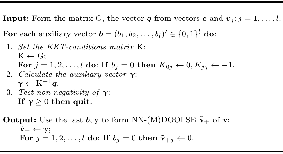 \n",
"\n",
"$~$\n",
">$\n",
"\\qquad \\mathbf{q} = \n",
"\\left(\\begin{array}{c}\n",
"\\mathbf{e}' \\mathbf{e}\\\\\n",
"(\\mathbf{e}' \\mathbf{v}_{1})^2 \\\\\n",
"\\vdots \\\\\n",
"(\\mathbf{e}' \\mathbf{v}_{l})^2\n",
"\\end{array}\\right)\n",
"$\n",
">\n",
"> $\\qquad\\mathrm{G} = \\left(\\begin{array}{ccccc}\n",
"\\small\n",
"n^* & ||\\mathbf{v}_{1}||^2 & ||\\mathbf{v}_{2}||^2 & \\ldots & ||\\mathbf{v}_{l}||^2 \\\\\n",
"||\\mathbf{v}_{1}||^2 & ||\\mathbf{v}_{1}||^4 & 0 & \\ldots & 0 \\\\\n",
"||\\mathbf{v}_{2}||^2 & 0 & ||\\mathbf{v}_{2}||^4 & \\ldots & 0 \\\\\n",
"\\vdots & \\vdots & \\vdots & \\ldots & \\vdots \\\\\n",
"||\\mathbf{v}_{l}||^2 & 0 & 0 & \\ldots & ||\\mathbf{v}_{l}||^4\n",
"\\end{array}\\right)\n",
"$"
]
},
{
"cell_type": "code",
"execution_count": 15,
"metadata": {},
"outputs": [],
"source": [
"# Input: form G\n",
"ns = n\n",
"u, v, Q = ns, matrix([nv2(j) for j in [1..l]]), diagonal_matrix([nv2(j)^2 for j in [1..l]])\n",
"G = block_matrix([[u,v],[v.T,Q]])"
]
},
{
"cell_type": "code",
"execution_count": 16,
"metadata": {},
"outputs": [],
"source": [
"# form q\n",
"e2, Ve2 = ec*e, (Vc*e).elementwise_product(Vc*e)\n",
"q = e2.stack(Ve2).expand()"
]
},
{
"cell_type": "code",
"execution_count": 17,
"metadata": {},
"outputs": [],
"source": [
"# body of the algorithm\n",
"for b in product([0,1], repeat=l+1): \n",
" # set the KKT-conditions matrix K\n",
" K = G*1\n",
" for j in range(l+1): \n",
" if b[j] == 1: K[0,j], K[j,j] = 0,-1\n",
" # calculate the auxiliary vector g\n",
" g = K^(-1)*q\n",
" # test non-negativity g\n",
" if RRk(min(g.list()))>=0: break "
]
},
{
"cell_type": "code",
"execution_count": 18,
"metadata": {},
"outputs": [
{
"data": {
"text/plain": [
"(\n",
"[0.92908798823403546177] \n",
"[ 2.8882933656238099623] \n",
"[ 1.6844347380982690249] \n",
"[0.29451097548641021445] \n",
"[ 1.7860554270569467631], (0, 0, 0, 0, 0)\n",
")"
]
},
"execution_count": 18,
"metadata": {},
"output_type": "execute_result"
}
],
"source": [
"RRk_matrix(K^(-1)*q), b"
]
},
{
"cell_type": "code",
"execution_count": 19,
"metadata": {},
"outputs": [],
"source": [
"# Output: Form estimates nu\n",
"nu = g*1\n",
"for j in range(l+1):\n",
" if b[j] == 1: nu[j] = 0"
]
},
{
"cell_type": "code",
"execution_count": 20,
"metadata": {},
"outputs": [
{
"data": {
"text/html": [
""
],
"text/plain": [
"[ -6569/4800*sqrt(3)*sqrt(2) - 13207/4800*sqrt(3) - 22533/8000*sqrt(2) + 312727/24000]\n",
"[ 6569/57600*sqrt(3)*sqrt(2) + 12499/11520*sqrt(3) + 7511/32000*sqrt(2) + 114553/288000]\n",
"[ 6569/57600*sqrt(3)*sqrt(2) + 42007/57600*sqrt(3) + 7511/32000*sqrt(2) - 54727/288000]\n",
"[ 6569/57600*sqrt(3)*sqrt(2) + 13207/57600*sqrt(3) + 11711/32000*sqrt(2) - 259067/288000]\n",
"[6569/57600*sqrt(3)*sqrt(2) + 13207/57600*sqrt(3) + 244759/288000*sqrt(2) - 26587/288000]"
]
},
"metadata": {},
"output_type": "display_data"
}
],
"source": [
"# final DOOLSE\n",
"DOOLSE = nu\n",
"show(DOOLSE)"
]
},
{
"cell_type": "code",
"execution_count": 21,
"metadata": {
"scrolled": true
},
"outputs": [
{
"name": "stdout",
"output_type": "stream",
"text": [
"([0.92908798823403546177]\n",
"[ 2.8882933656238099623]\n",
"[ 1.6844347380982690249]\n",
"[0.29451097548641021445]\n",
"[ 1.7860554270569467631], 3.9140125377802497, (0, 0, 0, 0, 0))\n"
]
}
],
"source": [
"# numerical results\n",
"DOOLSEnum = RRk_matrix(DOOLSE)\n",
"print(DOOLSEnum, DOOLSE.norm(),b)"
]
},
{
"cell_type": "markdown",
"metadata": {},
"source": [
"## $\\boldsymbol{2^{nd}}$ stage of EBLUP-NE"
]
},
{
"cell_type": "code",
"execution_count": 22,
"metadata": {
"scrolled": true
},
"outputs": [
{
"data": {
"text/html": [
""
],
"text/plain": [
"[ -6569/4080*sqrt(3)*sqrt(2) - 13207/4080*sqrt(3) - 22533/6800*sqrt(2) + 312727/20400]\n",
"[62903880404539/720000*sqrt(3)*sqrt(2)/(131623604*sqrt(3) + 227978887) + 118388172594739/480000*sqrt(3)/(131623604*sqrt(3) + 227978887) + 145262037326489/960000*sqrt(2)/(131623604*sqrt(3) + 227978887) + 2461639439072431/5760000/(131623604*sqrt(3) + 227978887)]\n",
"[ 470569623499/432000000*sqrt(3)*sqrt(2)/(2064*sqrt(3) + 3577) + 1508091636667/864000000*sqrt(3)/(2064*sqrt(3) + 3577) + 135307323803/72000000*sqrt(2)/(2064*sqrt(3) + 3577) + 1368780734167/432000000/(2064*sqrt(3) + 3577)]\n",
"[ -234034914761/28800*sqrt(3)*sqrt(2)/(10141740*sqrt(2) + 14342689) - 6635711343581/576000*sqrt(3)/(10141740*sqrt(2) + 14342689) + 3924718485263/240000*sqrt(2)/(10141740*sqrt(2) + 14342689) + 33727347602137/1440000/(10141740*sqrt(2) + 14342689)]\n",
"[ 5760245177807/48000*sqrt(3)*sqrt(2)/(253462812*sqrt(2) + 361618577) + 95155973057291/576000*sqrt(3)/(253462812*sqrt(2) + 361618577) + 17232911341513/80000*sqrt(2)/(253462812*sqrt(2) + 361618577) + 501009056253409/1440000/(253462812*sqrt(2) + 361618577)]"
]
},
"metadata": {},
"output_type": "display_data"
}
],
"source": [
"# final EBLUPNE based on DOOLSE\n",
"EBLUPNEsimp = EBLUPNE(DOOLSE).column().expand()\n",
"show(EBLUPNEsimp)"
]
},
{
"cell_type": "code",
"execution_count": 23,
"metadata": {},
"outputs": [
{
"data": {
"text/plain": [
"[ 1]\n",
"[0.94846887861963596617]\n",
"[0.91404212152622161047]\n",
"[0.62700200702811399302]\n",
"[0.91863007601174459834]"
]
},
"execution_count": 23,
"metadata": {},
"output_type": "execute_result"
}
],
"source": [
"# numerical results\n",
"rho2(DOOLSEnum).column()"
]
},
{
"cell_type": "code",
"execution_count": 24,
"metadata": {},
"outputs": [
{
"data": {
"text/plain": [
"[ 1.0930446920400417197]\n",
"[ 2.8128906231460250176]\n",
"[ 1.6104130979046378695]\n",
"[0.23320397549915796799]\n",
"[ 1.7118482468229312038]"
]
},
"execution_count": 24,
"metadata": {},
"output_type": "execute_result"
}
],
"source": [
"EBLUPNEnum = RRk_matrix(EBLUPNEsimp)\n",
"EBLUPNEnum "
]
},
{
"cell_type": "code",
"execution_count": 25,
"metadata": {},
"outputs": [
{
"data": {
"text/plain": [
"3.832145510914468"
]
},
"execution_count": 25,
"metadata": {},
"output_type": "execute_result"
}
],
"source": [
"EBLUPNEnum.norm()"
]
},
{
"cell_type": "markdown",
"metadata": {},
"source": [
"***\n",
"\n",
"# NN-DOOLSE or REMLE\n",
"using the KKT algorithm (tab.3, _Hancova et al 2019_)\n",
"\n",
"## $\\boldsymbol{1^{st}}$ stage of EBLUP-NE "
]
},
{
"cell_type": "code",
"execution_count": 26,
"metadata": {},
"outputs": [],
"source": [
"# Input: form G\n",
"ns = n-k\n",
"u, v, Q = ns, matrix([nv2(j) for j in [1..l]]), diagonal_matrix([nv2(j)^2 for j in [1..l]])\n",
"G = block_matrix([[u,v],[v.T,Q]])"
]
},
{
"cell_type": "code",
"execution_count": 27,
"metadata": {},
"outputs": [],
"source": [
"# form q\n",
"e2, Ve2 = ec*e, (Vc*e).elementwise_product(Vc*e)\n",
"q = e2.stack(Ve2).expand()"
]
},
{
"cell_type": "code",
"execution_count": 28,
"metadata": {},
"outputs": [],
"source": [
"# body of the algorithm\n",
"for b in product([0,1], repeat=l+1): \n",
" # set the KKT-conditions matrix K\n",
" K = G*1\n",
" for j in range(l+1): \n",
" if b[j] == 1: K[0,j], K[j,j] = 0,-1\n",
" # calculate the auxiliary vector g\n",
" g = K^(-1)*q\n",
" # test non-negativity g\n",
" if RRk(min(g.list()))>=0: break "
]
},
{
"cell_type": "code",
"execution_count": 29,
"metadata": {},
"outputs": [],
"source": [
"# Output: Form estimates nu\n",
"nu = g*1\n",
"for j in range(l+1):\n",
" if b[j] == 1: nu[j] = 0"
]
},
{
"cell_type": "code",
"execution_count": 30,
"metadata": {},
"outputs": [
{
"data": {
"text/html": [
""
],
"text/plain": [
"[ -6569/4080*sqrt(3)*sqrt(2) - 13207/4080*sqrt(3) - 22533/6800*sqrt(2) + 312727/20400]\n",
"[6569/48960*sqrt(3)*sqrt(2) + 275509/244800*sqrt(3) + 7511/27200*sqrt(2) + 50461/244800]\n",
"[ 6569/48960*sqrt(3)*sqrt(2) + 37687/48960*sqrt(3) + 7511/27200*sqrt(2) - 93427/244800]\n",
"[ 6569/48960*sqrt(3)*sqrt(2) + 13207/48960*sqrt(3) + 11081/27200*sqrt(2) - 66779/61200]\n",
"[ 6569/48960*sqrt(3)*sqrt(2) + 13207/48960*sqrt(3) + 43637/48960*sqrt(2) - 17377/61200]"
]
},
"metadata": {},
"output_type": "display_data"
}
],
"source": [
"# final MDOOLSE\n",
"MDOOLSE = nu\n",
"show(MDOOLSE)"
]
},
{
"cell_type": "code",
"execution_count": 31,
"metadata": {
"scrolled": true
},
"outputs": [
{
"name": "stdout",
"output_type": "stream",
"text": [
"([ 1.0930446920400417197]\n",
"[ 2.8746303069733094408]\n",
"[ 1.6707716794477685035]\n",
"[0.28084791683590969296]\n",
"[ 1.7723923684064462416], 3.933188829103883, (0, 0, 0, 0, 0))\n"
]
}
],
"source": [
"# numerical results\n",
"MDOOLSEnum = RRk_matrix(nu)\n",
"print(MDOOLSEnum, MDOOLSE.norm(),b)"
]
},
{
"cell_type": "markdown",
"metadata": {},
"source": [
"## $\\boldsymbol{2^{nd}}$ stage of EBLUP-NE"
]
},
{
"cell_type": "code",
"execution_count": 32,
"metadata": {
"scrolled": true
},
"outputs": [
{
"data": {
"text/html": [
""
],
"text/plain": [
"[ -6569/4080*sqrt(3)*sqrt(2) - 13207/4080*sqrt(3) - 22533/6800*sqrt(2) + 312727/20400]\n",
"[202458749967223/2080800*sqrt(3)*sqrt(2)/(131623604*sqrt(3) + 227978887) + 79446253773673/346800*sqrt(3)/(131623604*sqrt(3) + 227978887) + 29220340181009/173400*sqrt(2)/(131623604*sqrt(3) + 227978887) + 1652247156325153/4161600/(131623604*sqrt(3) + 227978887)]\n",
"[ 354914718049/312120000*sqrt(3)*sqrt(2)/(2064*sqrt(3) + 3577) + 1004299836367/624240000*sqrt(3)/(2064*sqrt(3) + 3577) + 50959492039/26010000*sqrt(2)/(2064*sqrt(3) + 3577) + 932870373217/312120000/(2064*sqrt(3) + 3577)]\n",
"[ -5365175547883/416160*sqrt(3)*sqrt(2)/(10141740*sqrt(2) + 14342689) - 760370956481/41616*sqrt(3)/(10141740*sqrt(2) + 14342689) + 8448017987833/346800*sqrt(2)/(10141740*sqrt(2) + 14342689) + 145067898730489/4161600/(10141740*sqrt(2) + 14342689)]\n",
"[ 17318024920831/138720*sqrt(3)*sqrt(2)/(253462812*sqrt(2) + 361618577) + 35419150072903/208080*sqrt(3)/(253462812*sqrt(2) + 361618577) + 67634307651191/346800*sqrt(2)/(253462812*sqrt(2) + 361618577) + 1404250908252913/4161600/(253462812*sqrt(2) + 361618577)]"
]
},
"metadata": {},
"output_type": "display_data"
}
],
"source": [
"# final EBLUPNE based on NE\n",
"EBLUPNEsimp = EBLUPNE(MDOOLSE).column().expand()\n",
"show(EBLUPNEsimp)"
]
},
{
"cell_type": "code",
"execution_count": 33,
"metadata": {},
"outputs": [
{
"data": {
"text/plain": [
"[ 1]\n",
"[0.93951664761802805166]\n",
"[0.89927400850167713940]\n",
"[0.57017526933078310576]\n",
"[0.90462906726347676354]"
]
},
"execution_count": 33,
"metadata": {},
"output_type": "execute_result"
}
],
"source": [
"# numerical results\n",
"rho2(MDOOLSEnum).column()"
]
},
{
"cell_type": "code",
"execution_count": 34,
"metadata": {},
"outputs": [
{
"data": {
"text/plain": [
"[ 1.0930446920400417197]\n",
"[ 2.7863408362122582278]\n",
"[ 1.5843937689416014278]\n",
"[0.21206812426244698957]\n",
"[ 1.6857576550762177074]"
]
},
"execution_count": 34,
"metadata": {},
"output_type": "execute_result"
}
],
"source": [
"EBLUPNEnum = RRk_matrix(EBLUPNEsimp)\n",
"EBLUPNEnum "
]
},
{
"cell_type": "code",
"execution_count": 35,
"metadata": {},
"outputs": [
{
"data": {
"text/plain": [
"3.78886491318682"
]
},
"execution_count": 35,
"metadata": {},
"output_type": "execute_result"
}
],
"source": [
"EBLUPNEnum.norm()"
]
},
{
"cell_type": "markdown",
"metadata": {},
"source": [
"***\n",
"\n",
"# References \n",
"This notebook belongs to suplementary materials of the paper submitted to Statistical Papers and available at .\n",
"\n",
"* Hančová, M., Vozáriková, G., Gajdoš, A., Hanč, J. (2019). [Estimating variance components in time series\n",
"\tlinear regression models using empirical BLUPs and convex optimization](https://arxiv.org/abs/1905.07771), https://arxiv.org/, 2019. \n",
"\n",
"### Abstract of the paper\n",
"\n",
"We propose a two-stage estimation method of variance components in time series models known as FDSLRMs, whose observations can be described by a linear mixed model (LMM). We based estimating variances, fundamental quantities in a time series forecasting approach called kriging, on the empirical (plug-in) best linear unbiased predictions of unobservable random components in FDSLRM. \n",
"\n",
"The method, providing invariant non-negative quadratic estimators, can be used for any absolutely continuous probability distribution of time series data. As a result of applying the convex optimization and the LMM methodology, we resolved two problems $-$ theoretical existence and equivalence between least squares estimators, non-negative (M)DOOLSE, and maximum likelihood estimators, (RE)MLE, as possible starting points of our method and a \n",
"practical lack of computational implementation for FDSLRM. As for computing (RE)MLE in the case of $ n $ observed time series values, we also discovered a new algorithm of order $\\mathcal{O}(n)$, which at the default precision is $10^7$ times more accurate and $n^2$ times faster than the best current Python(or R)-based computational packages, namely CVXPY, CVXR, nlme, sommer and mixed. \n",
"\n",
"We illustrate our results on three real data sets $-$ electricity consumption, tourism and cyber security $-$ which are easily available, reproducible, sharable and modifiable in the form of interactive Jupyter notebooks."
]
},
{
"cell_type": "markdown",
"metadata": {},
"source": [
"* Štulajter, F., Witkovský, V. (2004). [Estimation of Variances in Orthogonal Finite\n",
"Discrete Spectrum Linear Regression Models](https://link.springer.com/article/10.1007/s001840300299). _Metrika_, 2004, Vol. 60, No. 2, pp. 105–118"
]
},
{
"cell_type": "markdown",
"metadata": {},
"source": [
"| [Table of Contents](#table_of_contents) | [Data and model](#data_and_model) | [Natural estimators](#natural_estimators) | [NN-DOOLSE, MLE](#doolse) | [NN-MDOOLSE, REMLE](#mdoolse) | [References](#references) |"
]
}
],
"metadata": {
"kernelspec": {
"display_name": "SageMath 8.3",
"language": "",
"name": "sagemath"
},
"language_info": {
"codemirror_mode": {
"name": "ipython",
"version": 2
},
"file_extension": ".py",
"mimetype": "text/x-python",
"name": "python",
"nbconvert_exporter": "python",
"pygments_lexer": "ipython2",
"version": "2.7.15"
},
"varInspector": {
"cols": {
"lenName": 16,
"lenType": 16,
"lenVar": 40
},
"kernels_config": {
"python": {
"delete_cmd_postfix": "",
"delete_cmd_prefix": "del ",
"library": "var_list.py",
"varRefreshCmd": "print(var_dic_list())"
},
"r": {
"delete_cmd_postfix": ") ",
"delete_cmd_prefix": "rm(",
"library": "var_list.r",
"varRefreshCmd": "cat(var_dic_list()) "
}
},
"types_to_exclude": [
"module",
"function",
"builtin_function_or_method",
"instance",
"_Feature"
],
"window_display": false
}
},
"nbformat": 4,
"nbformat_minor": 2
}
\n",
"\n",
"$~$\n",
">$\n",
"\\qquad \\mathbf{q} = \n",
"\\left(\\begin{array}{c}\n",
"\\mathbf{e}' \\mathbf{e}\\\\\n",
"(\\mathbf{e}' \\mathbf{v}_{1})^2 \\\\\n",
"\\vdots \\\\\n",
"(\\mathbf{e}' \\mathbf{v}_{l})^2\n",
"\\end{array}\\right)\n",
"$\n",
">\n",
"> $\\qquad\\mathrm{G} = \\left(\\begin{array}{ccccc}\n",
"\\small\n",
"n^* & ||\\mathbf{v}_{1}||^2 & ||\\mathbf{v}_{2}||^2 & \\ldots & ||\\mathbf{v}_{l}||^2 \\\\\n",
"||\\mathbf{v}_{1}||^2 & ||\\mathbf{v}_{1}||^4 & 0 & \\ldots & 0 \\\\\n",
"||\\mathbf{v}_{2}||^2 & 0 & ||\\mathbf{v}_{2}||^4 & \\ldots & 0 \\\\\n",
"\\vdots & \\vdots & \\vdots & \\ldots & \\vdots \\\\\n",
"||\\mathbf{v}_{l}||^2 & 0 & 0 & \\ldots & ||\\mathbf{v}_{l}||^4\n",
"\\end{array}\\right)\n",
"$"
]
},
{
"cell_type": "code",
"execution_count": 15,
"metadata": {},
"outputs": [],
"source": [
"# Input: form G\n",
"ns = n\n",
"u, v, Q = ns, matrix([nv2(j) for j in [1..l]]), diagonal_matrix([nv2(j)^2 for j in [1..l]])\n",
"G = block_matrix([[u,v],[v.T,Q]])"
]
},
{
"cell_type": "code",
"execution_count": 16,
"metadata": {},
"outputs": [],
"source": [
"# form q\n",
"e2, Ve2 = ec*e, (Vc*e).elementwise_product(Vc*e)\n",
"q = e2.stack(Ve2).expand()"
]
},
{
"cell_type": "code",
"execution_count": 17,
"metadata": {},
"outputs": [],
"source": [
"# body of the algorithm\n",
"for b in product([0,1], repeat=l+1): \n",
" # set the KKT-conditions matrix K\n",
" K = G*1\n",
" for j in range(l+1): \n",
" if b[j] == 1: K[0,j], K[j,j] = 0,-1\n",
" # calculate the auxiliary vector g\n",
" g = K^(-1)*q\n",
" # test non-negativity g\n",
" if RRk(min(g.list()))>=0: break "
]
},
{
"cell_type": "code",
"execution_count": 18,
"metadata": {},
"outputs": [
{
"data": {
"text/plain": [
"(\n",
"[0.92908798823403546177] \n",
"[ 2.8882933656238099623] \n",
"[ 1.6844347380982690249] \n",
"[0.29451097548641021445] \n",
"[ 1.7860554270569467631], (0, 0, 0, 0, 0)\n",
")"
]
},
"execution_count": 18,
"metadata": {},
"output_type": "execute_result"
}
],
"source": [
"RRk_matrix(K^(-1)*q), b"
]
},
{
"cell_type": "code",
"execution_count": 19,
"metadata": {},
"outputs": [],
"source": [
"# Output: Form estimates nu\n",
"nu = g*1\n",
"for j in range(l+1):\n",
" if b[j] == 1: nu[j] = 0"
]
},
{
"cell_type": "code",
"execution_count": 20,
"metadata": {},
"outputs": [
{
"data": {
"text/html": [
""
],
"text/plain": [
"[ -6569/4800*sqrt(3)*sqrt(2) - 13207/4800*sqrt(3) - 22533/8000*sqrt(2) + 312727/24000]\n",
"[ 6569/57600*sqrt(3)*sqrt(2) + 12499/11520*sqrt(3) + 7511/32000*sqrt(2) + 114553/288000]\n",
"[ 6569/57600*sqrt(3)*sqrt(2) + 42007/57600*sqrt(3) + 7511/32000*sqrt(2) - 54727/288000]\n",
"[ 6569/57600*sqrt(3)*sqrt(2) + 13207/57600*sqrt(3) + 11711/32000*sqrt(2) - 259067/288000]\n",
"[6569/57600*sqrt(3)*sqrt(2) + 13207/57600*sqrt(3) + 244759/288000*sqrt(2) - 26587/288000]"
]
},
"metadata": {},
"output_type": "display_data"
}
],
"source": [
"# final DOOLSE\n",
"DOOLSE = nu\n",
"show(DOOLSE)"
]
},
{
"cell_type": "code",
"execution_count": 21,
"metadata": {
"scrolled": true
},
"outputs": [
{
"name": "stdout",
"output_type": "stream",
"text": [
"([0.92908798823403546177]\n",
"[ 2.8882933656238099623]\n",
"[ 1.6844347380982690249]\n",
"[0.29451097548641021445]\n",
"[ 1.7860554270569467631], 3.9140125377802497, (0, 0, 0, 0, 0))\n"
]
}
],
"source": [
"# numerical results\n",
"DOOLSEnum = RRk_matrix(DOOLSE)\n",
"print(DOOLSEnum, DOOLSE.norm(),b)"
]
},
{
"cell_type": "markdown",
"metadata": {},
"source": [
"## $\\boldsymbol{2^{nd}}$ stage of EBLUP-NE"
]
},
{
"cell_type": "code",
"execution_count": 22,
"metadata": {
"scrolled": true
},
"outputs": [
{
"data": {
"text/html": [
""
],
"text/plain": [
"[ -6569/4080*sqrt(3)*sqrt(2) - 13207/4080*sqrt(3) - 22533/6800*sqrt(2) + 312727/20400]\n",
"[62903880404539/720000*sqrt(3)*sqrt(2)/(131623604*sqrt(3) + 227978887) + 118388172594739/480000*sqrt(3)/(131623604*sqrt(3) + 227978887) + 145262037326489/960000*sqrt(2)/(131623604*sqrt(3) + 227978887) + 2461639439072431/5760000/(131623604*sqrt(3) + 227978887)]\n",
"[ 470569623499/432000000*sqrt(3)*sqrt(2)/(2064*sqrt(3) + 3577) + 1508091636667/864000000*sqrt(3)/(2064*sqrt(3) + 3577) + 135307323803/72000000*sqrt(2)/(2064*sqrt(3) + 3577) + 1368780734167/432000000/(2064*sqrt(3) + 3577)]\n",
"[ -234034914761/28800*sqrt(3)*sqrt(2)/(10141740*sqrt(2) + 14342689) - 6635711343581/576000*sqrt(3)/(10141740*sqrt(2) + 14342689) + 3924718485263/240000*sqrt(2)/(10141740*sqrt(2) + 14342689) + 33727347602137/1440000/(10141740*sqrt(2) + 14342689)]\n",
"[ 5760245177807/48000*sqrt(3)*sqrt(2)/(253462812*sqrt(2) + 361618577) + 95155973057291/576000*sqrt(3)/(253462812*sqrt(2) + 361618577) + 17232911341513/80000*sqrt(2)/(253462812*sqrt(2) + 361618577) + 501009056253409/1440000/(253462812*sqrt(2) + 361618577)]"
]
},
"metadata": {},
"output_type": "display_data"
}
],
"source": [
"# final EBLUPNE based on DOOLSE\n",
"EBLUPNEsimp = EBLUPNE(DOOLSE).column().expand()\n",
"show(EBLUPNEsimp)"
]
},
{
"cell_type": "code",
"execution_count": 23,
"metadata": {},
"outputs": [
{
"data": {
"text/plain": [
"[ 1]\n",
"[0.94846887861963596617]\n",
"[0.91404212152622161047]\n",
"[0.62700200702811399302]\n",
"[0.91863007601174459834]"
]
},
"execution_count": 23,
"metadata": {},
"output_type": "execute_result"
}
],
"source": [
"# numerical results\n",
"rho2(DOOLSEnum).column()"
]
},
{
"cell_type": "code",
"execution_count": 24,
"metadata": {},
"outputs": [
{
"data": {
"text/plain": [
"[ 1.0930446920400417197]\n",
"[ 2.8128906231460250176]\n",
"[ 1.6104130979046378695]\n",
"[0.23320397549915796799]\n",
"[ 1.7118482468229312038]"
]
},
"execution_count": 24,
"metadata": {},
"output_type": "execute_result"
}
],
"source": [
"EBLUPNEnum = RRk_matrix(EBLUPNEsimp)\n",
"EBLUPNEnum "
]
},
{
"cell_type": "code",
"execution_count": 25,
"metadata": {},
"outputs": [
{
"data": {
"text/plain": [
"3.832145510914468"
]
},
"execution_count": 25,
"metadata": {},
"output_type": "execute_result"
}
],
"source": [
"EBLUPNEnum.norm()"
]
},
{
"cell_type": "markdown",
"metadata": {},
"source": [
"***\n",
"\n",
"# NN-DOOLSE or REMLE\n",
"using the KKT algorithm (tab.3, _Hancova et al 2019_)\n",
"\n",
"## $\\boldsymbol{1^{st}}$ stage of EBLUP-NE "
]
},
{
"cell_type": "code",
"execution_count": 26,
"metadata": {},
"outputs": [],
"source": [
"# Input: form G\n",
"ns = n-k\n",
"u, v, Q = ns, matrix([nv2(j) for j in [1..l]]), diagonal_matrix([nv2(j)^2 for j in [1..l]])\n",
"G = block_matrix([[u,v],[v.T,Q]])"
]
},
{
"cell_type": "code",
"execution_count": 27,
"metadata": {},
"outputs": [],
"source": [
"# form q\n",
"e2, Ve2 = ec*e, (Vc*e).elementwise_product(Vc*e)\n",
"q = e2.stack(Ve2).expand()"
]
},
{
"cell_type": "code",
"execution_count": 28,
"metadata": {},
"outputs": [],
"source": [
"# body of the algorithm\n",
"for b in product([0,1], repeat=l+1): \n",
" # set the KKT-conditions matrix K\n",
" K = G*1\n",
" for j in range(l+1): \n",
" if b[j] == 1: K[0,j], K[j,j] = 0,-1\n",
" # calculate the auxiliary vector g\n",
" g = K^(-1)*q\n",
" # test non-negativity g\n",
" if RRk(min(g.list()))>=0: break "
]
},
{
"cell_type": "code",
"execution_count": 29,
"metadata": {},
"outputs": [],
"source": [
"# Output: Form estimates nu\n",
"nu = g*1\n",
"for j in range(l+1):\n",
" if b[j] == 1: nu[j] = 0"
]
},
{
"cell_type": "code",
"execution_count": 30,
"metadata": {},
"outputs": [
{
"data": {
"text/html": [
""
],
"text/plain": [
"[ -6569/4080*sqrt(3)*sqrt(2) - 13207/4080*sqrt(3) - 22533/6800*sqrt(2) + 312727/20400]\n",
"[6569/48960*sqrt(3)*sqrt(2) + 275509/244800*sqrt(3) + 7511/27200*sqrt(2) + 50461/244800]\n",
"[ 6569/48960*sqrt(3)*sqrt(2) + 37687/48960*sqrt(3) + 7511/27200*sqrt(2) - 93427/244800]\n",
"[ 6569/48960*sqrt(3)*sqrt(2) + 13207/48960*sqrt(3) + 11081/27200*sqrt(2) - 66779/61200]\n",
"[ 6569/48960*sqrt(3)*sqrt(2) + 13207/48960*sqrt(3) + 43637/48960*sqrt(2) - 17377/61200]"
]
},
"metadata": {},
"output_type": "display_data"
}
],
"source": [
"# final MDOOLSE\n",
"MDOOLSE = nu\n",
"show(MDOOLSE)"
]
},
{
"cell_type": "code",
"execution_count": 31,
"metadata": {
"scrolled": true
},
"outputs": [
{
"name": "stdout",
"output_type": "stream",
"text": [
"([ 1.0930446920400417197]\n",
"[ 2.8746303069733094408]\n",
"[ 1.6707716794477685035]\n",
"[0.28084791683590969296]\n",
"[ 1.7723923684064462416], 3.933188829103883, (0, 0, 0, 0, 0))\n"
]
}
],
"source": [
"# numerical results\n",
"MDOOLSEnum = RRk_matrix(nu)\n",
"print(MDOOLSEnum, MDOOLSE.norm(),b)"
]
},
{
"cell_type": "markdown",
"metadata": {},
"source": [
"## $\\boldsymbol{2^{nd}}$ stage of EBLUP-NE"
]
},
{
"cell_type": "code",
"execution_count": 32,
"metadata": {
"scrolled": true
},
"outputs": [
{
"data": {
"text/html": [
""
],
"text/plain": [
"[ -6569/4080*sqrt(3)*sqrt(2) - 13207/4080*sqrt(3) - 22533/6800*sqrt(2) + 312727/20400]\n",
"[202458749967223/2080800*sqrt(3)*sqrt(2)/(131623604*sqrt(3) + 227978887) + 79446253773673/346800*sqrt(3)/(131623604*sqrt(3) + 227978887) + 29220340181009/173400*sqrt(2)/(131623604*sqrt(3) + 227978887) + 1652247156325153/4161600/(131623604*sqrt(3) + 227978887)]\n",
"[ 354914718049/312120000*sqrt(3)*sqrt(2)/(2064*sqrt(3) + 3577) + 1004299836367/624240000*sqrt(3)/(2064*sqrt(3) + 3577) + 50959492039/26010000*sqrt(2)/(2064*sqrt(3) + 3577) + 932870373217/312120000/(2064*sqrt(3) + 3577)]\n",
"[ -5365175547883/416160*sqrt(3)*sqrt(2)/(10141740*sqrt(2) + 14342689) - 760370956481/41616*sqrt(3)/(10141740*sqrt(2) + 14342689) + 8448017987833/346800*sqrt(2)/(10141740*sqrt(2) + 14342689) + 145067898730489/4161600/(10141740*sqrt(2) + 14342689)]\n",
"[ 17318024920831/138720*sqrt(3)*sqrt(2)/(253462812*sqrt(2) + 361618577) + 35419150072903/208080*sqrt(3)/(253462812*sqrt(2) + 361618577) + 67634307651191/346800*sqrt(2)/(253462812*sqrt(2) + 361618577) + 1404250908252913/4161600/(253462812*sqrt(2) + 361618577)]"
]
},
"metadata": {},
"output_type": "display_data"
}
],
"source": [
"# final EBLUPNE based on NE\n",
"EBLUPNEsimp = EBLUPNE(MDOOLSE).column().expand()\n",
"show(EBLUPNEsimp)"
]
},
{
"cell_type": "code",
"execution_count": 33,
"metadata": {},
"outputs": [
{
"data": {
"text/plain": [
"[ 1]\n",
"[0.93951664761802805166]\n",
"[0.89927400850167713940]\n",
"[0.57017526933078310576]\n",
"[0.90462906726347676354]"
]
},
"execution_count": 33,
"metadata": {},
"output_type": "execute_result"
}
],
"source": [
"# numerical results\n",
"rho2(MDOOLSEnum).column()"
]
},
{
"cell_type": "code",
"execution_count": 34,
"metadata": {},
"outputs": [
{
"data": {
"text/plain": [
"[ 1.0930446920400417197]\n",
"[ 2.7863408362122582278]\n",
"[ 1.5843937689416014278]\n",
"[0.21206812426244698957]\n",
"[ 1.6857576550762177074]"
]
},
"execution_count": 34,
"metadata": {},
"output_type": "execute_result"
}
],
"source": [
"EBLUPNEnum = RRk_matrix(EBLUPNEsimp)\n",
"EBLUPNEnum "
]
},
{
"cell_type": "code",
"execution_count": 35,
"metadata": {},
"outputs": [
{
"data": {
"text/plain": [
"3.78886491318682"
]
},
"execution_count": 35,
"metadata": {},
"output_type": "execute_result"
}
],
"source": [
"EBLUPNEnum.norm()"
]
},
{
"cell_type": "markdown",
"metadata": {},
"source": [
"***\n",
"\n",
"# References \n",
"This notebook belongs to suplementary materials of the paper submitted to Statistical Papers and available at .\n",
"\n",
"* Hančová, M., Vozáriková, G., Gajdoš, A., Hanč, J. (2019). [Estimating variance components in time series\n",
"\tlinear regression models using empirical BLUPs and convex optimization](https://arxiv.org/abs/1905.07771), https://arxiv.org/, 2019. \n",
"\n",
"### Abstract of the paper\n",
"\n",
"We propose a two-stage estimation method of variance components in time series models known as FDSLRMs, whose observations can be described by a linear mixed model (LMM). We based estimating variances, fundamental quantities in a time series forecasting approach called kriging, on the empirical (plug-in) best linear unbiased predictions of unobservable random components in FDSLRM. \n",
"\n",
"The method, providing invariant non-negative quadratic estimators, can be used for any absolutely continuous probability distribution of time series data. As a result of applying the convex optimization and the LMM methodology, we resolved two problems $-$ theoretical existence and equivalence between least squares estimators, non-negative (M)DOOLSE, and maximum likelihood estimators, (RE)MLE, as possible starting points of our method and a \n",
"practical lack of computational implementation for FDSLRM. As for computing (RE)MLE in the case of $ n $ observed time series values, we also discovered a new algorithm of order $\\mathcal{O}(n)$, which at the default precision is $10^7$ times more accurate and $n^2$ times faster than the best current Python(or R)-based computational packages, namely CVXPY, CVXR, nlme, sommer and mixed. \n",
"\n",
"We illustrate our results on three real data sets $-$ electricity consumption, tourism and cyber security $-$ which are easily available, reproducible, sharable and modifiable in the form of interactive Jupyter notebooks."
]
},
{
"cell_type": "markdown",
"metadata": {},
"source": [
"* Štulajter, F., Witkovský, V. (2004). [Estimation of Variances in Orthogonal Finite\n",
"Discrete Spectrum Linear Regression Models](https://link.springer.com/article/10.1007/s001840300299). _Metrika_, 2004, Vol. 60, No. 2, pp. 105–118"
]
},
{
"cell_type": "markdown",
"metadata": {},
"source": [
"| [Table of Contents](#table_of_contents) | [Data and model](#data_and_model) | [Natural estimators](#natural_estimators) | [NN-DOOLSE, MLE](#doolse) | [NN-MDOOLSE, REMLE](#mdoolse) | [References](#references) |"
]
}
],
"metadata": {
"kernelspec": {
"display_name": "SageMath 8.3",
"language": "",
"name": "sagemath"
},
"language_info": {
"codemirror_mode": {
"name": "ipython",
"version": 2
},
"file_extension": ".py",
"mimetype": "text/x-python",
"name": "python",
"nbconvert_exporter": "python",
"pygments_lexer": "ipython2",
"version": "2.7.15"
},
"varInspector": {
"cols": {
"lenName": 16,
"lenType": 16,
"lenVar": 40
},
"kernels_config": {
"python": {
"delete_cmd_postfix": "",
"delete_cmd_prefix": "del ",
"library": "var_list.py",
"varRefreshCmd": "print(var_dic_list())"
},
"r": {
"delete_cmd_postfix": ") ",
"delete_cmd_prefix": "rm(",
"library": "var_list.r",
"varRefreshCmd": "cat(var_dic_list()) "
}
},
"types_to_exclude": [
"module",
"function",
"builtin_function_or_method",
"instance",
"_Feature"
],
"window_display": false
}
},
"nbformat": 4,
"nbformat_minor": 2
}