### A Pluto.jl notebook ###
# v0.20.4

using Markdown
using InteractiveUtils

# This Pluto notebook uses @bind for interactivity. When running this notebook outside of Pluto, the following 'mock version' of @bind gives bound variables a default value (instead of an error).
macro bind(def, element)
    #! format: off
    quote
        local iv = try Base.loaded_modules[Base.PkgId(Base.UUID("6e696c72-6542-2067-7265-42206c756150"), "AbstractPlutoDingetjes")].Bonds.initial_value catch; b -> missing; end
        local el = $(esc(element))
        global $(esc(def)) = Core.applicable(Base.get, el) ? Base.get(el) : iv(el)
        el
    end
    #! format: on
end

# ╔═╡ 36610294-87dc-11eb-21e8-5b1dd06c6020
begin
	using PlutoUI
	using Interpolations
	using Roots
	using LaTeXStrings
	using Plots
	using Optim
end

# ╔═╡ d367efe3-f2e1-40b2-8bd1-47bb827424d0
html"""
<style>
	main {
		margin: 0 auto;
		max-width: 2000px;
    	padding-left: max(160px, 10%);
    	padding-right: max(160px, 10%);
		font-size: x-large
	}
</style>
"""

# ╔═╡ 5fab5e80-87ce-11eb-111a-d5288227b97c
html"<button onclick='present()'>present</button>"

# ╔═╡ 705e96f2-87ce-11eb-3f5a-eb6cdb8c49d4
md"
# Dynamic Programming 2

> Florian Oswald, Carlo Alberto 2025


* In this notebook we'll add uncertainty to our simple setup from the last time.
* We'll stay in the finite time framework, but everything we say will be easily portable to infinite time. 
* We'll write code (of course). We won't worry about performance so far, but try to be as explicit as possible.
* We'll do something that looks reasonable but works terribly. 
* Then we'll fix it and celebrate! 🎉


"

# ╔═╡ 34403942-87d2-11eb-1172-7bd285bf7d75
md"
#

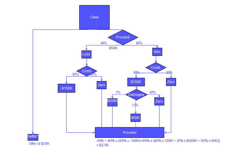
* A good place to start is a so called decision tree. 
![](https://upload.wikimedia.org/wikipedia/commons/4/48/DecisionCalcs.jpg)"

# ╔═╡ b9ed265e-87d2-11eb-1028-05b4c4ccbc74
md"

## Markov Decision Problems (MDPs)

* Assume a finite set of states $S$
* A finite set of actions $A$
* For state $s\in S$ and action $a \in A$ we can compute the *cost* or the *contribution* $C(s,a)$
* There is a *transition matrix* $p_t(S_{t+1} | S_{t}, a_t)$ which tells us with which probability we go from state $S_{t}$ to $S_{t+1}$ upen taking decision $a_t$
* Even though many problems have *continuous* state and action spaces, this is a very useful class of problems to study.
"

# ╔═╡ 07992abe-87d4-11eb-0fd7-1bef7fc2ada8
md"
## Optimality (Bellman) Equations

* But let's start with _no uncertainty_. If we are at state $S_t$, we know how $S_{t+1}$ will look like with certainty if we choose a certain action $a_t$ 
* Then we just choose the best action:
$$a_t^*(S_t) = \arg \max_{a_t \in A_t} \left(C_t(S_t,a_t) + \beta V_{t+1}(S_{t+1}(S_t,a_t)) \right)$$
* The associated *value* of this choice is then the same Bellman Equation we know from last time,
$$\begin{align}V_t(S_t) &= \max_{a_t \in A_t} \left(C_t(S_t,a_t) + \beta V_{t+1}(S_{t+1}(S_t,a_t)) \right) \\ &= C_t(S_t,a^*_t(S_t)) + \beta V_{t+1}(S_{t+1}(S_t,a^*_t(S_t)))\end{align}$$
"

# ╔═╡ 93148b06-87d2-11eb-2356-fb460acf8e66
md"

## Enter Uncertainty

* Uncertainty comes into play if we *don't know exactly what state* $S_{t+1}$ we'll end up in.
* We may have partial information on the likelihood of each state occuring, like a belief, or prior information.
* We have our transition matrix $p_t(S_{t+1} | S_{t}, a_t)$, and can define the *standard form of the Bellman Equation*:

$$V_t(S_t) = \max_{a_t \in A_t} \left(C_t(S_t,a_t) + \beta \sum_{s' \in S} p_t\left( S_{t+1} = s' | S_t, a_t \right)V_{t+1}(s') \right)$$
"

# ╔═╡ 3d97787a-87d2-11eb-3713-ab3dad6e5e8b
md"
#

* we can also write it more general without the summation
$$V_t(S_t) = \max_{a_t \in A_t} \left(C_t(S_t,a_t) + \beta \mathbb{E} \left[ V_{t+1}(S_{t+1}(S_t,a_t)) | S_t \right] \right)$$"

# ╔═╡ a41aff3a-87d8-11eb-00fe-e16c14870ba2
md"

## Let's Do it!

* Let's look at this specific problem where the *action* is *consumption*, and $u$ is a *utility function* and the state is $R_t$:
$$V_t(R_t) = \max_{0 \leq c_t \leq R_t} \left(u(c_t) + \beta \mathbb{E} \left[ V_{t+1}(R_{t+1}(R_t,c_t)) |R_t \right] \right)$$

* Here $R_t$ could be available cash on hand of the consumer.
* Let us specify a *law of motion* for the state as 
$$R_{t+1} = R_t - c_t + y_{t+1}$$ where $y_t$ is a random variable.
* We have to compute expectations wrt to $y$

"

# ╔═╡ c6ed3824-87d9-11eb-3e0a-b5a473fdb952
md"

## I.I.D. Shock

* Let's start with the simplest case: $y_t \in \{\overline{y}, \underline{y}\}, 0 < \overline{y} < \underline{y}$
* There is a probability π associated to $P(y = \overline{y}) = \pi$
* There is *no state dependence* in the $y$ process: the current $y_t$ does not matter for the future $y_{t+1}$

"

# ╔═╡ 51983542-87f9-11eb-226a-81fe383f0763
md"
#
"

# ╔═╡ 6ddfc91c-87da-11eb-3b5c-dfe006576f29
"""
	Bellman(grid::Vector,vplus::Vector,π::Float64,yvec::Vector)

Given a grid and a next period value function `vplus`, and a probability distribution
calculate current period optimal value and actions.
"""
function Bellman(grid::Vector,vplus::Vector,π::Float64,yvec::Vector{Float64},β::Float64)
	points = length(grid)
	w = zeros(points) # temporary vector for each choice or R'
	Vt = zeros(points) # optimal value in T-1 at each state of R
	ix = 0 # optimal action index in T-1 at each state of R
	at = zeros(points) # optimal action in T-1 at each state of R

	for (ir,r) in enumerate(grid) # for all possible R-values
		# loop over all possible action choices
		for (ia,achoice) in enumerate(grid)
			if r <= achoice   # check whether that choice is feasible
				w[ia] = -Inf
			else
				rlow = r - achoice + yvec[1] # tomorrow's R if y is low
				rhigh  = r - achoice + yvec[2] # tomorrow's R if y is high
				jlow = argmin(abs.(grid .- rlow))  # index of that value in Rspace
				jhigh = argmin(abs.(grid .- rhigh))  # index of that value in Rspace
				w[ia] = sqrt(achoice) + β * ((1-π) * vplus[jlow] + (π) * vplus[jhigh] ) # value of that achoice
			end
		end
		# find best action
		Vt[ir], ix = findmax(w) # stores Value und policy (index of optimal choice)
		at[ir] = grid[ix]  # record optimal action level
	end
	return (Vt, at)
end

# ╔═╡ aeb2b692-87db-11eb-3c9a-114acdc3d159
md"
#
"

# ╔═╡ b3f20522-87db-11eb-325d-7ba201c66452
begin
	points = 500
	lowR = 0.01
	highR = 10.0
	# more points towards zero to make nicer plot
	Rspace = exp.(range(log(lowR), stop = log(highR), length = points))
	aT = Rspace # consume whatever is left
	VT = sqrt.(aT)  # utility of that consumption
	yvec = [1.0, 3.0]
	nperiods = 10
	β = 1.0  # irrelevant for now
	π = 0.7
end

# ╔═╡ 6e8aec5e-87f9-11eb-2e53-bf5ba90fa750
md"
#
"

# ╔═╡ f00890ee-87db-11eb-153d-bb9244b46e89
# identical
function backwards(grid, nperiods, β, π, yvec)
	points = length(grid)
	V = zeros(nperiods,points)
	c = zeros(nperiods,points)
	V[end,:] = sqrt.(grid)  # from before: final period
	c[end,:] = collect(grid)

	for it in (nperiods-1):-1:1
		x = Bellman(grid, V[it+1,:], π, yvec, β)	
		V[it,:] = x[1]
		c[it,:] = x[2]
	end
	return (V,c)
end

# ╔═╡ 4da91e08-87dc-11eb-3238-433fbdda7df7
V,a = backwards(Rspace, nperiods, β, π, yvec);

# ╔═╡ 7a97ba6a-87f9-11eb-1c88-a999bcff4647
md"
#
"

# ╔═╡ ca3e6b12-87dc-11eb-31c6-8d3be744def0
let
	cg = cgrad(:viridis)
    cols = cg[range(0.0,stop=1.0,length = nperiods)]
	pa = plot(Rspace, a[1,:], xlab = "R", ylab = "Action",label = L"a_1",leg = :topleft, color = cols[1])
	for it in 2:nperiods
		plot!(pa, Rspace, a[it,:], label = L"a_{%$(it)}", color = cols[it])
	end
	pv = plot(Rspace, V[1,:], xlab = "R", ylab = "Value",label = L"V_1",leg = :bottomright, color = cols[1])
	for it in 2:nperiods
		plot!(pv, Rspace, V[it,:], label = L"V_{%$(it)}", color = cols[it])
	end
	plot(pv,pa, layout = (1,2))
end

# ╔═╡ 027875e0-87e0-11eb-0ca5-317b58b0f8fc
PlutoUI.Resource("https://i.ytimg.com/vi/wAbnNZDhYrA/maxresdefault.jpg")

# ╔═╡ 48cc5fa2-87dd-11eb-309b-9708941fd8d5
md"
#

* Oh wow! That's like...total disaster!
* 😩
* This way of interpolating the future value function does *not work very well*
* Let's use proper interpolation instead!
* Instead of `vplus[jlow]` we want to have `vplus[Rprime]` where `Rprime` $\in \mathbb{R}$!

#

"

# ╔═╡ 04b6c4b8-87df-11eb-21dd-15a443042bd1
"""
	Bellman(grid::Vector,vplus::Vector,π::Float64,yvec::Vector)

Given a grid and a next period value function `vplus`, and a probability distribution
calculate current period optimal value and actions.
"""
function Bellman2(grid::Vector,vplus::Vector,π::Float64,yvec::Vector,β::Float64)
	points = length(grid)
	w = zeros(points) # temporary vector for each choice or R'
	Vt = zeros(points) # optimal value in T-1 at each state of R
	ix = 0 # optimal action index in T-1 at each state of R
	at = zeros(points) # optimal action in T-1 at each state of R
	
	# interpolator
	vitp = interpolate((grid,), vplus, Gridded(Linear()))
	vitp = extrapolate(vitp, Interpolations.Flat())

	for (ir,r) in enumerate(grid) # for all possible R-values
		# loop over all possible action choices
		for (ia,achoice) in enumerate(grid)
			if r <= achoice   # check whether that choice is feasible
				w[ia] = -Inf
			else
				rlow = r - achoice + yvec[1] # tomorrow's R if y is low
				rhigh  = r - achoice + yvec[2] # tomorrow's R if y is high
				w[ia] = sqrt(achoice) + (1-π) * vitp(rlow) + (π) * vitp(rhigh)  # value of that achoice
			end
		end
		# find best action
		Vt[ir], ix = findmax(w) # stores Value und policy (index of optimal choice)
		at[ir] = grid[ix]  # record optimal action level
	end
	return (Vt, at)
end

# ╔═╡ 99b19ed4-92c8-11eb-2daa-2df3db8736bd
md"
#
"

# ╔═╡ 43539482-87e0-11eb-22c8-b9380ae1ebdb
function backwards2(grid, nperiods, π, yvec, β)
	points = length(grid)
	V = zeros(nperiods,points)
	a = zeros(nperiods,points)
	V[end,:] = sqrt.(grid)  # from before: final period
	a[end,:] = collect(grid)

	for it in (nperiods-1):-1:1
		x = Bellman2(grid, V[it+1,:], π, yvec, β)	
		V[it,:] = x[1]
		a[it,:] = x[2]
	end
	return (V,a)
end

# ╔═╡ a361963a-92c8-11eb-0543-7decc61720a8
md"
#
"

# ╔═╡ 5f764692-87df-11eb-3b9d-e5823eb4d1b3
let
	V,a = backwards2(Rspace,nperiods,π,yvec,β)
	cg = cgrad(:viridis)
    cols = cg[range(0.0,stop=1.0,length = nperiods)]
	pa = plot(Rspace, a[1,:], xlab = "R", ylab = "Action",label = L"a_1",leg = :topleft, color = cols[1])
	for it in 2:nperiods
		plot!(pa, Rspace, a[it,:], label = L"a_{%$(it)}", color = cols[it])
	end
	pv = plot(Rspace, V[1,:], xlab = "R", ylab = "Value",label = L"V_1",leg = :bottomright, color = cols[1])
	for it in 2:nperiods
		plot!(pv, Rspace, V[it,:], label = L"V_{%$(it)}", color = cols[it])
	end
	plot(pv,pa, layout = (1,2))
end

# ╔═╡ 8eb731f6-87e0-11eb-35dd-61ba070afc8b
md"

#

* Well at least a little bit better. 
* Still, what about those steps in there? What's going on?
"

# ╔═╡ 02d26410-87e2-11eb-0278-99ee0bbd2923
md"

## Continuous Choice

* In fact our action space is continuous here:
$$V_t(R_t) = \max_{0 \leq a_t \leq R_t} \left(u(a_t) + \beta \mathbb{E} \left[ V_{t+1}(R_{t+1}(R_t,a_t)) |R_t \right] \right)$$

* So let's treat it as such. We could direct optimization for the Bellman Operator!

#

"

# ╔═╡ 3b1f5120-87e2-11eb-1b10-85900b6fbeb6
function bellman3(grid,v0,β::Float64, π, yvec)
    n = length(v0)
    v1  = zeros(n)     # next guess
    pol = zeros(n)     # consumption policy function

    Interp = interpolate((collect(grid),), v0, Gridded(Linear()) ) 
    Interp = extrapolate(Interp,Interpolations.Flat())

    # loop over current states
    # of current resources
    for (i,r) in enumerate(grid)

        objective(c) = - (sqrt.(c) + β * (π * Interp(r - c + yvec[2]) + (1-π) * Interp(r - c + yvec[1])) )
        res = optimize(objective, 1e-6, r)  # search in [1e-6,r]
        pol[i] = res.minimizer
        v1[i] = -res.minimum
    end
    return (v1,pol)   # return both value and policy function
end


# ╔═╡ c6990bb0-92c8-11eb-2523-9f8a7ec1cd4a
md"
#
"

# ╔═╡ 0b83e920-87e3-11eb-0792-479eb843b429
function backwards3(grid, nperiods,β, π, yvec)
	points = length(grid)
	V = zeros(nperiods,points)
	a = zeros(nperiods,points)
	V[end,:] = sqrt.(grid)  # from before: final period
	a[end,:] = collect(grid)

	for it in (nperiods-1):-1:1
		x = bellman3(grid, V[it+1,:],β,  π, yvec)	
		V[it,:] = x[1]
		a[it,:] = x[2]
	end
	return (V,a)
end

# ╔═╡ d391139e-92c8-11eb-0888-b325a75fb10f
md"
#
"

# ╔═╡ 7003b4e8-87e3-11eb-28a9-f7e3668beac3
let
	V,a = backwards3(Rspace,nperiods,β,π,yvec)
	cg = cgrad(:viridis)
    cols = cg[range(0.0,stop=1.0,length = nperiods)]
	pa = plot(Rspace, a[1,:], xlab = "R", ylab = "Action",label = L"a_1",leg = :topleft, color = cols[1])
	for it in 2:nperiods
		plot!(pa, Rspace, a[it,:], label = L"a_{%$(it)}", color = cols[it])
	end
	pv = plot(Rspace, V[1,:], xlab = "R", ylab = "Value",label = L"V_1",leg = :bottomright, color = cols[1])
	for it in 2:nperiods
		plot!(pv, Rspace, V[it,:], label = L"V_{%$(it)}", color = cols[it])
	end
	plot(pv,pa, layout = (1,2))
end

# ╔═╡ 4504d988-87e4-11eb-05d5-c9f9f215f785
md"

#

* It's getting there!
* Much fewer wiggles in the consumption function.
* But we can do even better than that.
* Let's do *Policy Iteration* rather than *Value Iteration*!
"

# ╔═╡ 6828b538-87e4-11eb-3cdd-71c31dad5a6e
md"

## Policy Iteration

* In most economic contexts, there is more structure on a problem.
* In our consumption example, we know that the Euler Equation must hold.
* Sometimes there are other *optimality conditions* that one could leverage.
* In our case, we have this equation at an optimal policy $c^*(R_t)$:
$$\begin{align}
u'(c^*(R_t)) & = \beta \mathbb{E} \left[ u'(c(R_{t+1})) \right] \\
             & = \beta \mathbb{E} \left[ u'(R_t - c^*(R_t) + y)   \right]
\end{align}$$
* So: We *just* have to find the function $c^*(R_t)$!
"

# ╔═╡ ba19759c-87eb-11eb-1bec-51de9ac10e31
md"

## *Just*?

* There is a slight issue here. The Euler Equation in itself does not enforce the contraint that we cannot borrow any $R$. 
* In particular, $R_{t} \geq 0$ is missing from the above equation.
* look back above at the last plot of the consumption function. It has a kink!
* The Euler Equation applies only to the *right* of that kink!
* If tomorrow's consumption is low (we are saving a lot), today's consumption is relatively high, implying that we consume more than we have in terms of $R_t$.
* Satisfying the Euler Equation would require to set $R_t <0$ sometimes, which is ruled out.


"

# ╔═╡ a4018f28-87ec-11eb-07f0-af86523dd26e
md"
#

* So if we want to use the Euler Equation, we need to manually adjust for that.
* 😩
* Alright, let's do it. It's not too bad in the end.

#

* First, let's put down the marginal utility function and it's inverse:

"

# ╔═╡ 027fda74-87f1-11eb-1441-55d6e410bf4c
u_prime(c) = 0.5 .* c.^(-0.5)

# ╔═╡ 540d8814-87f1-11eb-0b8c-23357c46f93c
u_primeinv(u) = (2 .* u).^(-2)

# ╔═╡ d2788ffe-92c4-11eb-19e7-4b41d9f9ebdd
md"

#

* We need the _inverse_ of the marginal utility function?
* Yes. Here is why. For any candidate consumption level $c_t$
$$\begin{align}
u'(c_t) & = \beta \mathbb{E} \left[ u'(c(R_{t+1})) \right] \\
u'(c_t) & = \text{RHS}
\end{align}$$
* So, if we have computed the RHS, current period optimal consumption is just
$$c_t  = \left( u' \right)^{-1}\left(\text{RHS}\right)\hspace{1cm}(\text{EEresid})$$

where $\left( u' \right)^{-1}(z)$ denotes the _inverse_ of function $u'(x)$. 

#

### Example

* Suppose tomorrow's consumption function _does_ have the kink at $R_{t+1} = 1.5$
* I.e. $c_{t+1}^*(R_{t+1}) = R_{t+1},\forall R_{t+1} \leq 1.5$
* Let $y_{t+1} = 1.5, R_t = 1$. Now try out consumption choice $c_t = 1$!

$$\begin{align}
R_{t+1} &= R_t - c_t+ y_{t+1} \\
        &= 1 - 1 + 1.5 = 1.5 \\
\Rightarrow c_{t+1}^*(1.5) &= 1.5
\end{align}$$ 

because right at the kink! 
* Then, the Euler equation says: 
$$\begin{align}
u'(c_t) & = u'(c_{t+1}) \\
c_t & = (u')^{-1}\left(u'(c_{t+1})\right) \\
c_t & = c_{t+1} = 1.5
\end{align}$$
* Well, that in turn means that $R_t - c_t = 1 - 1.5 < 0$, i.e. we would have to borrow 0.5 units of $R$ in order to satisfy that Euler Equation!

#
"

# ╔═╡ c75eed74-87ee-11eb-3e9a-3b893294baec
function EEresid(ct::Number,        # candidate current (t) consumption choice 
		         Rt::Number,        # current level of resources
				 cfunplus::Vector,  # next period's consumption *function*
		         grid::Vector,      # grid values on which cfunplus is defined
				 yvec::Vector,      # vector of values for shock
		         β::Number,         # discount factor
				 π::Number)         # prob of high y
	
	# next period resources, given candidate choice ct
	Rplus = Rt - ct .+ yvec  # a (2,1) vector: Rplus for each income level

	# get implied next period consumption from cplus
	# we add point (0,0) here to make sure that this is part of the grid.
	citp = extrapolate(
				interpolate(([0.0, grid...],), [0.0,cfunplus...], Gridded(Linear())), Interpolations.Flat())
	cplus = citp.(Rplus)
	RHS = β * [1-π  π] * u_prime(cplus) # expecte marginal utility of tomorrows consumption
	
	# euler residual: expression EEresid from above
	r = ct .- u_primeinv(RHS)
	r[1]  # array of size 1
end    

# ╔═╡ ae56f4e2-87f9-11eb-10fc-e3eda66e8a1f
md"
#
"

# ╔═╡ 17ea7f6a-87e7-11eb-2d3e-b9a1e771b08e
function policy_iter(grid,c0,u_prime,β::Float64, π, yvec)
    
    c1  = zeros(length(grid))     # next guess
    # loop over current states
    # of current resources
    for (i,r) in enumerate(grid)
		# get euler residual if we consume all resources
		res = EEresid(r,r,c0, grid, yvec,β , π)
		if res < 0
			# we consume too little today, c_t is too small for the Euler Equation.
			# could only make it bigger by borrowing next period.
			# but we cant! so really we are consuming all we have:
			c1[i] = r
		else
			# no problem here: Euler Equation holds
			# just need to find that ct that makes it zero:
			c1[i] = fzero( x-> EEresid(x,r,c0, grid, yvec, β, π) , 1e-6, r)
		end
    end
    return c1
end

# ╔═╡ bcca454c-87f9-11eb-0670-0d85db6b6e37
md"
#
"

# ╔═╡ c1e65340-87f9-11eb-3cd7-05f14edf71d2
md"
#
"

# ╔═╡ 6fbaac56-87e0-11eb-3d09-39a4fd293e88
PlutoUI.Resource("https://s3.getstickerpack.com/storage/uploads/sticker-pack/meme-pack-1/sticker_19.png?363e7ee56d4d8ad53813dae0907ef4c0&d=200x200")

# ╔═╡ a510ff40-9302-11eb-091e-6929367f6783
md"

# Infinite Time Problems

* Let's now introduce the infinite time version of this.
* For that purpose, let's rely on the well known Optimal Growth model:

$$\begin{align}
   V(k) &= \max_{0<k'<f(k)} u(f(k) - k') + \beta V(k')\\
  f(k)  & = k^\alpha\\
  k_0   & \text{ given} 
\end{align}$$

* The solution in finite time was simple by going backwards.
* Here, we need to rely on results from Functional Analysis: Remember the Contraction Mapping Theorem?
* The Contraction Mapping Theorem or the [Banache Fixed Point Theoreom](https://en.wikipedia.org/wiki/Banach_fixed-point_theorem) says there is a unique fixed point in an appropriately chosen function space. We arrive at it from an *arbitrary* starting point by just iterating on the operator $T(V)$ until $V = T(V)$
"


# ╔═╡ 06ff3932-9304-11eb-07cc-d798d56c0931
md"

# Implementing Value Function Iteration

### Checklist

1. Set parameter values
1. define a grid for state variable $k \in [0,2]$
1. initialize value function $V$
1. start iteration, repeatedly computing a new version of $V$.
1. stop if $d(V^{r},V^{r-1}) < \text{tol}$.
1. plot value and policy function 
1. report the maximum error of both wrt to analytic solution

#
"

# ╔═╡ 2e121c60-9304-11eb-29c4-afd0a289343f
begin
	alpha     = 0.65
	beta      = 0.95
	grid_max  = 2  # upper bound of capital grid
	n         = 150  # number of grid points
	N_iter    = 3000  # number of iterations
	kgrid     = 1e-2:(grid_max-1e-2)/(n-1):grid_max  # equispaced grid
	f(x) = x^alpha  # defines the production function f(k)
	tol = 1e-9
end

# ╔═╡ 3c8e560a-9304-11eb-2c45-7df67768f75b
md"

## Analytic Solution

* If we choose $u(x)=\ln(x)$, the problem has a closed form solution.
* We can use this to check accuracy of our solution.
"

# ╔═╡ 4849479a-9304-11eb-1c06-4b53a4163f85
begin 
	ab        = alpha * beta
	c1        = (log(1 - ab) + log(ab) * ab / (1 - ab)) / (1 - beta)
	c2        = alpha / (1 - ab)
	# optimal analytical values
	v_star(k) = c1 .+ c2 .* log.(k)  
	k_star(k) = ab * k.^alpha   
	c_star(k) = (1-ab) * k.^alpha  
	ufun(x) = log.(x)
end

# ╔═╡ 5984cd7a-9304-11eb-0bd4-ebac2da4f300
md"
#
"

# ╔═╡ 5d642bca-9304-11eb-2b23-dfa47b04bb22
# Bellman Operator
# inputs
# `grid`: grid of values of state variable
# `v0`: current guess of value function

# output
# `v1`: next guess of value function
# `pol`: corresponding policy function 

#takes a grid of state variables and computes the next iterate of the value function.
function bellman_operator(grid,v0)
    
    v1  = zeros(n)     # next guess
    pol = zeros(Int,n)     # policy function
    w   = zeros(n)   # temporary vector 

    # loop over current states
    # current capital
    for (i,k) in enumerate(grid)

        # loop over all possible kprime choices
        for (iprime,kprime) in enumerate(grid)
            if f(k) - kprime < 0   #check for negative consumption
                w[iprime] = -Inf
            else
                w[iprime] = ufun(f(k) - kprime) + beta * v0[iprime]
            end
        end
        # find maximal choice
        v1[i], pol[i] = findmax(w)     # stores Value und policy (index of optimal choice)
    end
    return (v1,grid[pol])   # return both value and policy function
end

# ╔═╡ 67d367c4-9304-11eb-0bfc-21b9bfec2fb9
md"
#
"

# ╔═╡ 6b33c6ca-9304-11eb-3766-fdcc42b64f2d
# VFI iterator
#
## input
# `n`: number of grid points
# output
# `v_next`: tuple with value and policy functions after `n` iterations.
function VFI(op::Function)
    v_init = zeros(n)     # initial guess
    for iter in 1:N_iter
        v_next = op(kgrid,v_init)  # returns a tuple: (v1,pol)
        # check convergence
        if maximum(abs,v_init.-v_next[1]) < tol
            verrors = maximum(abs,v_next[1].-v_star(kgrid))
            perrors = maximum(abs,v_next[2].-k_star(kgrid))
            return (v = v_next[1], p =v_next[2], errv = verrors, errp = perrors, iter = iter)
        elseif iter==N_iter
            @warn "No solution found after $iter iterations"
            return (v = v_next[1], p =v_next[2], errv = verrors, errp = perrors, iter = iter)
        end
        v_init = v_next[1]  # update guess 
    end
end



# ╔═╡ 72cc3cdc-9304-11eb-3548-95962c3513ec
md"
#
"

# ╔═╡ 776c4712-9304-11eb-1824-a14cde26b895
function plotVFI(v::NamedTuple)
    
    p = Any[]
	    # errors of both
	if eltype(v.p) == Int
		policy = kgrid[v.p]
	else
		policy = v.p
	end
    
    # value and policy functions
	if !isnan(v.v[1])
		push!(p,plot(kgrid,v.v,
            leg = false,title = "Vfun iterations: $(v.iter)",
            ylim=(-50,-30)))
		push!(p,plot(kgrid,v.v .- v_star(kgrid),
        title = "max Vfun error: $(round(v.errv,digits=3))"))
		perrors = policy .- k_star(kgrid)
	else
		push!(p,plot(title = "Vfun iterations: $(v.iter)"), plot())
		perrors = policy .- c_star(kgrid)
		
	end
    push!(p,plot(kgrid,policy,
            title = "policy function"))
    push!(p,plot(kgrid,perrors,
        title = "max policy error: $(round(v.errp,digits=3))"))

    plot(p...,layout=grid(2,2) , leg = false)
    
end

# ╔═╡ 7999a272-9304-11eb-254c-af591bae0620
plotVFI(VFI(bellman_operator))

# ╔═╡ a4ba5a96-ad59-4319-bd94-636f525853c6
function VFI_converge(op::Function,steps)
    v_init = zeros(n)     # initial guess
	pl = plot(kgrid, v_star(kgrid), color = :red, label = "true")
    for iter in 1:steps
		plot!(pl, kgrid, v_init, label = "", color = :grey)
        v_next = op(kgrid,v_init)  # returns a tuple: (v1,pol)
        # check convergence
        if maximum(abs,v_init.-v_next[1]) < tol
            verrors = maximum(abs,v_next[1].-v_star(kgrid))
            perrors = maximum(abs,v_next[2].-k_star(kgrid))
            return (v = v_next[1], p =v_next[2], errv = verrors, errp = perrors, iter = iter)
        elseif iter==N_iter
            @warn "No solution found after $iter iterations"
            return (v = v_next[1], p =v_next[2], errv = verrors, errp = perrors, iter = iter)
        end
        v_init = v_next[1]  # update guess 
    end
	pl
end

# ╔═╡ d52d3d31-e447-4120-92ae-3d4da7a02219
md"""
steps = $(@bind stps Slider(1:100, show_value = true, default = 1))
"""

# ╔═╡ c881819e-ca81-40b0-9e0f-93abcb43a2b4
VFI_converge(bellman_operator, stps)

# ╔═╡ 84e23d2a-9388-11eb-2483-3342d1683129
md"

## continous choice

* like before, now let's treat the choice dimension as a continuous variable
* This is almost identical to before with finite time.

#
"

# ╔═╡ 7e0a9d82-9304-11eb-1d3d-bb47fc55d033
function bellman_operator2(grid,v0)
    
    v1  = zeros(n)     # next guess
    pol = zeros(n)     # consumption policy function

    Interp = interpolate((collect(grid),), v0, Gridded(Linear()) ) 
    Interp = extrapolate(Interp,Interpolations.Flat())

    # loop over current states
    # of current capital
    for (i,k) in enumerate(grid)

        objective(c) = - (log.(c) + beta * Interp(f(k) - c))
        # find max of ojbective between [0,k^alpha]
        res = optimize(objective, 1e-6, f(k))  # Optim.jl
        pol[i] = f(k) - res.minimizer   # k'
        v1[i] = -res.minimum
    end
    return (v1,pol)   # return both value and policy function
end

# ╔═╡ aa891724-9388-11eb-32bb-8f8d15dc3761
md"
#
"

# ╔═╡ 597080ba-9307-11eb-2780-87474bfc5cff
plotVFI(VFI(bellman_operator2))

# ╔═╡ 6f9b2b8a-9389-11eb-2731-398e1342538a
md"
#

* Finally, policy function iteration!
* Again, remember the euler Equation here.

#
"

# ╔═╡ 710a0212-9307-11eb-2cf3-e75b9c5eddab
begin
	uprime(x) = 1.0 ./ x
	fprime(x) = alpha * x.^(alpha-1)
end

# ╔═╡ 67c4bbb8-9307-11eb-3ecb-13d7af9d899a
function policy_iter(grid,c0,u_prime,f_prime)

	c1  = zeros(length(grid))     # next guess
	pol_fun = extrapolate(interpolate((collect(grid),), c0, Gridded(Linear()) ) , Interpolations.Flat())

	# loop over current states
	# of current capital
	for (i,k) in enumerate(grid)
		objective(c) = u_prime(c) - beta * u_prime(pol_fun(f(k)-c)) * f_prime(f(k)-c)
		c1[i] = fzero(objective, 1e-10, f(k)-1e-10) 
	end
	return c1
end



# ╔═╡ d18511ea-87e7-11eb-08ce-a9176a32fbd1
function backwards_pol(grid, nperiods,β, π, yvec)
	u_prime(c) = 0.5 * c^(-0.5)
	points = length(grid)
	V = zeros(nperiods,points)
	c = zeros(nperiods,points)
	c[end,:] = collect(grid)
	V[end,:] = sqrt.(c[end,:] )  

	for it in (nperiods-1):-1:1
		c[it,:] = policy_iter(grid, c[it+1,:], u_prime, β,  π, yvec)
		# now calulate implied value function
		v_fun = extrapolate(interpolate((collect(grid),), V[it+1,:], Gridded(Linear()) ) , Interpolations.Flat())
		V[it,:] = sqrt.(c[it,:]) + β * ((1-π) * v_fun(grid .- c[it,:] .+ yvec[1]) + (π) * v_fun(grid .- c[it,:] .+ yvec[2]))
	end
	return (V,c)
end

# ╔═╡ c339ad8a-87e7-11eb-2802-0991af7b2a78
let
	V,a = backwards_pol(Rspace,nperiods,β,π,yvec)
	cg = cgrad(:viridis)
    cols = cg[range(0.0,stop=1.0,length = nperiods)]
	pa = plot(Rspace, a[1,:], xlab = "R", ylab = "Action",label = L"a_1",leg = :topleft, color = cols[1])
	for it in 2:nperiods
		plot!(pa, Rspace, a[it,:], label = L"a_{%$(it)}", color = cols[it])
	end
	pv = plot(Rspace, V[1,:], xlab = "R", ylab = "Value",label = L"V_1",leg = :bottomright, color = cols[1])
	for it in 2:nperiods
		plot!(pv, Rspace, V[it,:], label = L"V_{%$(it)}", color = cols[it])
	end
	plot(pv,pa, layout = (1,2))
end

# ╔═╡ 96a55b70-9389-11eb-13a1-3146098e9cb9
md"

#

"

# ╔═╡ 7b137330-9307-11eb-2644-390cd9c1e569
function PFI()
    c_init = kgrid
    for iter in 1:N_iter
        c_next = policy_iter(kgrid,c_init,uprime,fprime)  
        # check convergence
        if maximum(abs,c_init.-c_next) < tol
            perrors =  maximum(abs,c_next.-c_star(kgrid))
            return (v = fill(NaN,n), p =c_next, errv = 0.0, errp = perrors, iter = iter)

        elseif iter==N_iter
            warn("No solution found after $iter iterations")
            return (v = fill(NaN,n), p =c_next, errv = 0.0, errp = perrors, iter = iter)
        end
        c_init = c_next  # update guess 
    end
end

# ╔═╡ 9d4211e6-9389-11eb-03a4-559460e28c44
md"
#
"

# ╔═╡ 3b50f766-9386-11eb-2101-97a38644fda8
plotVFI(PFI())

# ╔═╡ 00000000-0000-0000-0000-000000000001
PLUTO_PROJECT_TOML_CONTENTS = """
[deps]
Interpolations = "a98d9a8b-a2ab-59e6-89dd-64a1c18fca59"
LaTeXStrings = "b964fa9f-0449-5b57-a5c2-d3ea65f4040f"
Optim = "429524aa-4258-5aef-a3af-852621145aeb"
Plots = "91a5bcdd-55d7-5caf-9e0b-520d859cae80"
PlutoUI = "7f904dfe-b85e-4ff6-b463-dae2292396a8"
Roots = "f2b01f46-fcfa-551c-844a-d8ac1e96c665"

[compat]
Interpolations = "~0.15.1"
LaTeXStrings = "~1.3.1"
Optim = "~1.9.3"
Plots = "~1.40.2"
PlutoUI = "~0.7.58"
Roots = "~2.1.5"
"""

# ╔═╡ 00000000-0000-0000-0000-000000000002
PLUTO_MANIFEST_TOML_CONTENTS = """
# This file is machine-generated - editing it directly is not advised

julia_version = "1.11.3"
manifest_format = "2.0"
project_hash = "f4838b632704daf6274629a2255fe274e10391fc"

[[deps.AbstractPlutoDingetjes]]
deps = ["Pkg"]
git-tree-sha1 = "6e1d2a35f2f90a4bc7c2ed98079b2ba09c35b83a"
uuid = "6e696c72-6542-2067-7265-42206c756150"
version = "1.3.2"

[[deps.Accessors]]
deps = ["CompositionsBase", "ConstructionBase", "InverseFunctions", "LinearAlgebra", "MacroTools", "Markdown"]
git-tree-sha1 = "b392ede862e506d451fc1616e79aa6f4c673dab8"
uuid = "7d9f7c33-5ae7-4f3b-8dc6-eff91059b697"
version = "0.1.38"

    [deps.Accessors.extensions]
    AccessorsAxisKeysExt = "AxisKeys"
    AccessorsDatesExt = "Dates"
    AccessorsIntervalSetsExt = "IntervalSets"
    AccessorsStaticArraysExt = "StaticArrays"
    AccessorsStructArraysExt = "StructArrays"
    AccessorsTestExt = "Test"
    AccessorsUnitfulExt = "Unitful"

    [deps.Accessors.weakdeps]
    AxisKeys = "94b1ba4f-4ee9-5380-92f1-94cde586c3c5"
    Dates = "ade2ca70-3891-5945-98fb-dc099432e06a"
    IntervalSets = "8197267c-284f-5f27-9208-e0e47529a953"
    Requires = "ae029012-a4dd-5104-9daa-d747884805df"
    StaticArrays = "90137ffa-7385-5640-81b9-e52037218182"
    StructArrays = "09ab397b-f2b6-538f-b94a-2f83cf4a842a"
    Test = "8dfed614-e22c-5e08-85e1-65c5234f0b40"
    Unitful = "1986cc42-f94f-5a68-af5c-568840ba703d"

[[deps.Adapt]]
deps = ["LinearAlgebra", "Requires"]
git-tree-sha1 = "50c3c56a52972d78e8be9fd135bfb91c9574c140"
uuid = "79e6a3ab-5dfb-504d-930d-738a2a938a0e"
version = "4.1.1"
weakdeps = ["StaticArrays"]

    [deps.Adapt.extensions]
    AdaptStaticArraysExt = "StaticArrays"

[[deps.ArgTools]]
uuid = "0dad84c5-d112-42e6-8d28-ef12dabb789f"
version = "1.1.2"

[[deps.ArrayInterface]]
deps = ["Adapt", "LinearAlgebra"]
git-tree-sha1 = "3640d077b6dafd64ceb8fd5c1ec76f7ca53bcf76"
uuid = "4fba245c-0d91-5ea0-9b3e-6abc04ee57a9"
version = "7.16.0"

    [deps.ArrayInterface.extensions]
    ArrayInterfaceBandedMatricesExt = "BandedMatrices"
    ArrayInterfaceBlockBandedMatricesExt = "BlockBandedMatrices"
    ArrayInterfaceCUDAExt = "CUDA"
    ArrayInterfaceCUDSSExt = "CUDSS"
    ArrayInterfaceChainRulesExt = "ChainRules"
    ArrayInterfaceGPUArraysCoreExt = "GPUArraysCore"
    ArrayInterfaceReverseDiffExt = "ReverseDiff"
    ArrayInterfaceSparseArraysExt = "SparseArrays"
    ArrayInterfaceStaticArraysCoreExt = "StaticArraysCore"
    ArrayInterfaceTrackerExt = "Tracker"

    [deps.ArrayInterface.weakdeps]
    BandedMatrices = "aae01518-5342-5314-be14-df237901396f"
    BlockBandedMatrices = "ffab5731-97b5-5995-9138-79e8c1846df0"
    CUDA = "052768ef-5323-5732-b1bb-66c8b64840ba"
    CUDSS = "45b445bb-4962-46a0-9369-b4df9d0f772e"
    ChainRules = "082447d4-558c-5d27-93f4-14fc19e9eca2"
    GPUArraysCore = "46192b85-c4d5-4398-a991-12ede77f4527"
    ReverseDiff = "37e2e3b7-166d-5795-8a7a-e32c996b4267"
    SparseArrays = "2f01184e-e22b-5df5-ae63-d93ebab69eaf"
    StaticArraysCore = "1e83bf80-4336-4d27-bf5d-d5a4f845583c"
    Tracker = "9f7883ad-71c0-57eb-9f7f-b5c9e6d3789c"

[[deps.Artifacts]]
uuid = "56f22d72-fd6d-98f1-02f0-08ddc0907c33"
version = "1.11.0"

[[deps.AxisAlgorithms]]
deps = ["LinearAlgebra", "Random", "SparseArrays", "WoodburyMatrices"]
git-tree-sha1 = "01b8ccb13d68535d73d2b0c23e39bd23155fb712"
uuid = "13072b0f-2c55-5437-9ae7-d433b7a33950"
version = "1.1.0"

[[deps.Base64]]
uuid = "2a0f44e3-6c83-55bd-87e4-b1978d98bd5f"
version = "1.11.0"

[[deps.BitFlags]]
git-tree-sha1 = "0691e34b3bb8be9307330f88d1a3c3f25466c24d"
uuid = "d1d4a3ce-64b1-5f1a-9ba4-7e7e69966f35"
version = "0.1.9"

[[deps.Bzip2_jll]]
deps = ["Artifacts", "JLLWrappers", "Libdl", "Pkg"]
git-tree-sha1 = "8873e196c2eb87962a2048b3b8e08946535864a1"
uuid = "6e34b625-4abd-537c-b88f-471c36dfa7a0"
version = "1.0.8+2"

[[deps.Cairo_jll]]
deps = ["Artifacts", "Bzip2_jll", "CompilerSupportLibraries_jll", "Fontconfig_jll", "FreeType2_jll", "Glib_jll", "JLLWrappers", "LZO_jll", "Libdl", "Pixman_jll", "Xorg_libXext_jll", "Xorg_libXrender_jll", "Zlib_jll", "libpng_jll"]
git-tree-sha1 = "009060c9a6168704143100f36ab08f06c2af4642"
uuid = "83423d85-b0ee-5818-9007-b63ccbeb887a"
version = "1.18.2+1"

[[deps.ChainRulesCore]]
deps = ["Compat", "LinearAlgebra"]
git-tree-sha1 = "3e4b134270b372f2ed4d4d0e936aabaefc1802bc"
uuid = "d360d2e6-b24c-11e9-a2a3-2a2ae2dbcce4"
version = "1.25.0"
weakdeps = ["SparseArrays"]

    [deps.ChainRulesCore.extensions]
    ChainRulesCoreSparseArraysExt = "SparseArrays"

[[deps.CodecZlib]]
deps = ["TranscodingStreams", "Zlib_jll"]
git-tree-sha1 = "bce6804e5e6044c6daab27bb533d1295e4a2e759"
uuid = "944b1d66-785c-5afd-91f1-9de20f533193"
version = "0.7.6"

[[deps.ColorSchemes]]
deps = ["ColorTypes", "ColorVectorSpace", "Colors", "FixedPointNumbers", "PrecompileTools", "Random"]
git-tree-sha1 = "13951eb68769ad1cd460cdb2e64e5e95f1bf123d"
uuid = "35d6a980-a343-548e-a6ea-1d62b119f2f4"
version = "3.27.0"

[[deps.ColorTypes]]
deps = ["FixedPointNumbers", "Random"]
git-tree-sha1 = "b10d0b65641d57b8b4d5e234446582de5047050d"
uuid = "3da002f7-5984-5a60-b8a6-cbb66c0b333f"
version = "0.11.5"

[[deps.ColorVectorSpace]]
deps = ["ColorTypes", "FixedPointNumbers", "LinearAlgebra", "Requires", "Statistics", "TensorCore"]
git-tree-sha1 = "a1f44953f2382ebb937d60dafbe2deea4bd23249"
uuid = "c3611d14-8923-5661-9e6a-0046d554d3a4"
version = "0.10.0"
weakdeps = ["SpecialFunctions"]

    [deps.ColorVectorSpace.extensions]
    SpecialFunctionsExt = "SpecialFunctions"

[[deps.Colors]]
deps = ["ColorTypes", "FixedPointNumbers", "Reexport"]
git-tree-sha1 = "64e15186f0aa277e174aa81798f7eb8598e0157e"
uuid = "5ae59095-9a9b-59fe-a467-6f913c188581"
version = "0.13.0"

[[deps.CommonSolve]]
git-tree-sha1 = "0eee5eb66b1cf62cd6ad1b460238e60e4b09400c"
uuid = "38540f10-b2f7-11e9-35d8-d573e4eb0ff2"
version = "0.2.4"

[[deps.CommonSubexpressions]]
deps = ["MacroTools"]
git-tree-sha1 = "cda2cfaebb4be89c9084adaca7dd7333369715c5"
uuid = "bbf7d656-a473-5ed7-a52c-81e309532950"
version = "0.3.1"

[[deps.Compat]]
deps = ["TOML", "UUIDs"]
git-tree-sha1 = "8ae8d32e09f0dcf42a36b90d4e17f5dd2e4c4215"
uuid = "34da2185-b29b-5c13-b0c7-acf172513d20"
version = "4.16.0"
weakdeps = ["Dates", "LinearAlgebra"]

    [deps.Compat.extensions]
    CompatLinearAlgebraExt = "LinearAlgebra"

[[deps.CompilerSupportLibraries_jll]]
deps = ["Artifacts", "Libdl"]
uuid = "e66e0078-7015-5450-92f7-15fbd957f2ae"
version = "1.1.1+0"

[[deps.CompositionsBase]]
git-tree-sha1 = "802bb88cd69dfd1509f6670416bd4434015693ad"
uuid = "a33af91c-f02d-484b-be07-31d278c5ca2b"
version = "0.1.2"
weakdeps = ["InverseFunctions"]

    [deps.CompositionsBase.extensions]
    CompositionsBaseInverseFunctionsExt = "InverseFunctions"

[[deps.ConcurrentUtilities]]
deps = ["Serialization", "Sockets"]
git-tree-sha1 = "ea32b83ca4fefa1768dc84e504cc0a94fb1ab8d1"
uuid = "f0e56b4a-5159-44fe-b623-3e5288b988bb"
version = "2.4.2"

[[deps.ConstructionBase]]
git-tree-sha1 = "76219f1ed5771adbb096743bff43fb5fdd4c1157"
uuid = "187b0558-2788-49d3-abe0-74a17ed4e7c9"
version = "1.5.8"

    [deps.ConstructionBase.extensions]
    ConstructionBaseIntervalSetsExt = "IntervalSets"
    ConstructionBaseLinearAlgebraExt = "LinearAlgebra"
    ConstructionBaseStaticArraysExt = "StaticArrays"

    [deps.ConstructionBase.weakdeps]
    IntervalSets = "8197267c-284f-5f27-9208-e0e47529a953"
    LinearAlgebra = "37e2e46d-f89d-539d-b4ee-838fcccc9c8e"
    StaticArrays = "90137ffa-7385-5640-81b9-e52037218182"

[[deps.Contour]]
git-tree-sha1 = "439e35b0b36e2e5881738abc8857bd92ad6ff9a8"
uuid = "d38c429a-6771-53c6-b99e-75d170b6e991"
version = "0.6.3"

[[deps.DataAPI]]
git-tree-sha1 = "abe83f3a2f1b857aac70ef8b269080af17764bbe"
uuid = "9a962f9c-6df0-11e9-0e5d-c546b8b5ee8a"
version = "1.16.0"

[[deps.DataStructures]]
deps = ["Compat", "InteractiveUtils", "OrderedCollections"]
git-tree-sha1 = "1d0a14036acb104d9e89698bd408f63ab58cdc82"
uuid = "864edb3b-99cc-5e75-8d2d-829cb0a9cfe8"
version = "0.18.20"

[[deps.Dates]]
deps = ["Printf"]
uuid = "ade2ca70-3891-5945-98fb-dc099432e06a"
version = "1.11.0"

[[deps.Dbus_jll]]
deps = ["Artifacts", "Expat_jll", "JLLWrappers", "Libdl"]
git-tree-sha1 = "fc173b380865f70627d7dd1190dc2fce6cc105af"
uuid = "ee1fde0b-3d02-5ea6-8484-8dfef6360eab"
version = "1.14.10+0"

[[deps.DelimitedFiles]]
deps = ["Mmap"]
git-tree-sha1 = "9e2f36d3c96a820c678f2f1f1782582fcf685bae"
uuid = "8bb1440f-4735-579b-a4ab-409b98df4dab"
version = "1.9.1"

[[deps.DiffResults]]
deps = ["StaticArraysCore"]
git-tree-sha1 = "782dd5f4561f5d267313f23853baaaa4c52ea621"
uuid = "163ba53b-c6d8-5494-b064-1a9d43ac40c5"
version = "1.1.0"

[[deps.DiffRules]]
deps = ["IrrationalConstants", "LogExpFunctions", "NaNMath", "Random", "SpecialFunctions"]
git-tree-sha1 = "23163d55f885173722d1e4cf0f6110cdbaf7e272"
uuid = "b552c78f-8df3-52c6-915a-8e097449b14b"
version = "1.15.1"

[[deps.Distributed]]
deps = ["Random", "Serialization", "Sockets"]
uuid = "8ba89e20-285c-5b6f-9357-94700520ee1b"
version = "1.11.0"

[[deps.DocStringExtensions]]
deps = ["LibGit2"]
git-tree-sha1 = "2fb1e02f2b635d0845df5d7c167fec4dd739b00d"
uuid = "ffbed154-4ef7-542d-bbb7-c09d3a79fcae"
version = "0.9.3"

[[deps.Downloads]]
deps = ["ArgTools", "FileWatching", "LibCURL", "NetworkOptions"]
uuid = "f43a241f-c20a-4ad4-852c-f6b1247861c6"
version = "1.6.0"

[[deps.EpollShim_jll]]
deps = ["Artifacts", "JLLWrappers", "Libdl"]
git-tree-sha1 = "8e9441ee83492030ace98f9789a654a6d0b1f643"
uuid = "2702e6a9-849d-5ed8-8c21-79e8b8f9ee43"
version = "0.0.20230411+0"

[[deps.ExceptionUnwrapping]]
deps = ["Test"]
git-tree-sha1 = "dcb08a0d93ec0b1cdc4af184b26b591e9695423a"
uuid = "460bff9d-24e4-43bc-9d9f-a8973cb893f4"
version = "0.1.10"

[[deps.Expat_jll]]
deps = ["Artifacts", "JLLWrappers", "Libdl"]
git-tree-sha1 = "1c6317308b9dc757616f0b5cb379db10494443a7"
uuid = "2e619515-83b5-522b-bb60-26c02a35a201"
version = "2.6.2+0"

[[deps.FFMPEG]]
deps = ["FFMPEG_jll"]
git-tree-sha1 = "53ebe7511fa11d33bec688a9178fac4e49eeee00"
uuid = "c87230d0-a227-11e9-1b43-d7ebe4e7570a"
version = "0.4.2"

[[deps.FFMPEG_jll]]
deps = ["Artifacts", "Bzip2_jll", "FreeType2_jll", "FriBidi_jll", "JLLWrappers", "LAME_jll", "Libdl", "Ogg_jll", "OpenSSL_jll", "Opus_jll", "PCRE2_jll", "Zlib_jll", "libaom_jll", "libass_jll", "libfdk_aac_jll", "libvorbis_jll", "x264_jll", "x265_jll"]
git-tree-sha1 = "466d45dc38e15794ec7d5d63ec03d776a9aff36e"
uuid = "b22a6f82-2f65-5046-a5b2-351ab43fb4e5"
version = "4.4.4+1"

[[deps.FileWatching]]
uuid = "7b1f6079-737a-58dc-b8bc-7a2ca5c1b5ee"
version = "1.11.0"

[[deps.FillArrays]]
deps = ["LinearAlgebra"]
git-tree-sha1 = "6a70198746448456524cb442b8af316927ff3e1a"
uuid = "1a297f60-69ca-5386-bcde-b61e274b549b"
version = "1.13.0"

    [deps.FillArrays.extensions]
    FillArraysPDMatsExt = "PDMats"
    FillArraysSparseArraysExt = "SparseArrays"
    FillArraysStatisticsExt = "Statistics"

    [deps.FillArrays.weakdeps]
    PDMats = "90014a1f-27ba-587c-ab20-58faa44d9150"
    SparseArrays = "2f01184e-e22b-5df5-ae63-d93ebab69eaf"
    Statistics = "10745b16-79ce-11e8-11f9-7d13ad32a3b2"

[[deps.FiniteDiff]]
deps = ["ArrayInterface", "LinearAlgebra", "Setfield"]
git-tree-sha1 = "b10bdafd1647f57ace3885143936749d61638c3b"
uuid = "6a86dc24-6348-571c-b903-95158fe2bd41"
version = "2.26.0"

    [deps.FiniteDiff.extensions]
    FiniteDiffBandedMatricesExt = "BandedMatrices"
    FiniteDiffBlockBandedMatricesExt = "BlockBandedMatrices"
    FiniteDiffSparseArraysExt = "SparseArrays"
    FiniteDiffStaticArraysExt = "StaticArrays"

    [deps.FiniteDiff.weakdeps]
    BandedMatrices = "aae01518-5342-5314-be14-df237901396f"
    BlockBandedMatrices = "ffab5731-97b5-5995-9138-79e8c1846df0"
    SparseArrays = "2f01184e-e22b-5df5-ae63-d93ebab69eaf"
    StaticArrays = "90137ffa-7385-5640-81b9-e52037218182"

[[deps.FixedPointNumbers]]
deps = ["Statistics"]
git-tree-sha1 = "05882d6995ae5c12bb5f36dd2ed3f61c98cbb172"
uuid = "53c48c17-4a7d-5ca2-90c5-79b7896eea93"
version = "0.8.5"

[[deps.Fontconfig_jll]]
deps = ["Artifacts", "Bzip2_jll", "Expat_jll", "FreeType2_jll", "JLLWrappers", "Libdl", "Libuuid_jll", "Zlib_jll"]
git-tree-sha1 = "db16beca600632c95fc8aca29890d83788dd8b23"
uuid = "a3f928ae-7b40-5064-980b-68af3947d34b"
version = "2.13.96+0"

[[deps.Format]]
git-tree-sha1 = "9c68794ef81b08086aeb32eeaf33531668d5f5fc"
uuid = "1fa38f19-a742-5d3f-a2b9-30dd87b9d5f8"
version = "1.3.7"

[[deps.ForwardDiff]]
deps = ["CommonSubexpressions", "DiffResults", "DiffRules", "LinearAlgebra", "LogExpFunctions", "NaNMath", "Preferences", "Printf", "Random", "SpecialFunctions"]
git-tree-sha1 = "a9ce73d3c827adab2d70bf168aaece8cce196898"
uuid = "f6369f11-7733-5829-9624-2563aa707210"
version = "0.10.37"
weakdeps = ["StaticArrays"]

    [deps.ForwardDiff.extensions]
    ForwardDiffStaticArraysExt = "StaticArrays"

[[deps.FreeType2_jll]]
deps = ["Artifacts", "Bzip2_jll", "JLLWrappers", "Libdl", "Zlib_jll"]
git-tree-sha1 = "5c1d8ae0efc6c2e7b1fc502cbe25def8f661b7bc"
uuid = "d7e528f0-a631-5988-bf34-fe36492bcfd7"
version = "2.13.2+0"

[[deps.FriBidi_jll]]
deps = ["Artifacts", "JLLWrappers", "Libdl"]
git-tree-sha1 = "1ed150b39aebcc805c26b93a8d0122c940f64ce2"
uuid = "559328eb-81f9-559d-9380-de523a88c83c"
version = "1.0.14+0"

[[deps.Future]]
deps = ["Random"]
uuid = "9fa8497b-333b-5362-9e8d-4d0656e87820"
version = "1.11.0"

[[deps.GLFW_jll]]
deps = ["Artifacts", "JLLWrappers", "Libdl", "Libglvnd_jll", "Xorg_libXcursor_jll", "Xorg_libXi_jll", "Xorg_libXinerama_jll", "Xorg_libXrandr_jll", "libdecor_jll", "xkbcommon_jll"]
git-tree-sha1 = "532f9126ad901533af1d4f5c198867227a7bb077"
uuid = "0656b61e-2033-5cc2-a64a-77c0f6c09b89"
version = "3.4.0+1"

[[deps.GR]]
deps = ["Artifacts", "Base64", "DelimitedFiles", "Downloads", "GR_jll", "HTTP", "JSON", "Libdl", "LinearAlgebra", "Preferences", "Printf", "Qt6Wayland_jll", "Random", "Serialization", "Sockets", "TOML", "Tar", "Test", "p7zip_jll"]
git-tree-sha1 = "ee28ddcd5517d54e417182fec3886e7412d3926f"
uuid = "28b8d3ca-fb5f-59d9-8090-bfdbd6d07a71"
version = "0.73.8"

[[deps.GR_jll]]
deps = ["Artifacts", "Bzip2_jll", "Cairo_jll", "FFMPEG_jll", "Fontconfig_jll", "FreeType2_jll", "GLFW_jll", "JLLWrappers", "JpegTurbo_jll", "Libdl", "Libtiff_jll", "Pixman_jll", "Qt6Base_jll", "Zlib_jll", "libpng_jll"]
git-tree-sha1 = "f31929b9e67066bee48eec8b03c0df47d31a74b3"
uuid = "d2c73de3-f751-5644-a686-071e5b155ba9"
version = "0.73.8+0"

[[deps.Gettext_jll]]
deps = ["Artifacts", "CompilerSupportLibraries_jll", "JLLWrappers", "Libdl", "Libiconv_jll", "Pkg", "XML2_jll"]
git-tree-sha1 = "9b02998aba7bf074d14de89f9d37ca24a1a0b046"
uuid = "78b55507-aeef-58d4-861c-77aaff3498b1"
version = "0.21.0+0"

[[deps.Glib_jll]]
deps = ["Artifacts", "Gettext_jll", "JLLWrappers", "Libdl", "Libffi_jll", "Libiconv_jll", "Libmount_jll", "PCRE2_jll", "Zlib_jll"]
git-tree-sha1 = "674ff0db93fffcd11a3573986e550d66cd4fd71f"
uuid = "7746bdde-850d-59dc-9ae8-88ece973131d"
version = "2.80.5+0"

[[deps.Graphite2_jll]]
deps = ["Artifacts", "JLLWrappers", "Libdl", "Pkg"]
git-tree-sha1 = "344bf40dcab1073aca04aa0df4fb092f920e4011"
uuid = "3b182d85-2403-5c21-9c21-1e1f0cc25472"
version = "1.3.14+0"

[[deps.Grisu]]
git-tree-sha1 = "53bb909d1151e57e2484c3d1b53e19552b887fb2"
uuid = "42e2da0e-8278-4e71-bc24-59509adca0fe"
version = "1.0.2"

[[deps.HTTP]]
deps = ["Base64", "CodecZlib", "ConcurrentUtilities", "Dates", "ExceptionUnwrapping", "Logging", "LoggingExtras", "MbedTLS", "NetworkOptions", "OpenSSL", "Random", "SimpleBufferStream", "Sockets", "URIs", "UUIDs"]
git-tree-sha1 = "bc3f416a965ae61968c20d0ad867556367f2817d"
uuid = "cd3eb016-35fb-5094-929b-558a96fad6f3"
version = "1.10.9"

[[deps.HarfBuzz_jll]]
deps = ["Artifacts", "Cairo_jll", "Fontconfig_jll", "FreeType2_jll", "Glib_jll", "Graphite2_jll", "JLLWrappers", "Libdl", "Libffi_jll"]
git-tree-sha1 = "401e4f3f30f43af2c8478fc008da50096ea5240f"
uuid = "2e76f6c2-a576-52d4-95c1-20adfe4de566"
version = "8.3.1+0"

[[deps.Hyperscript]]
deps = ["Test"]
git-tree-sha1 = "179267cfa5e712760cd43dcae385d7ea90cc25a4"
uuid = "47d2ed2b-36de-50cf-bf87-49c2cf4b8b91"
version = "0.0.5"

[[deps.HypertextLiteral]]
deps = ["Tricks"]
git-tree-sha1 = "7134810b1afce04bbc1045ca1985fbe81ce17653"
uuid = "ac1192a8-f4b3-4bfe-ba22-af5b92cd3ab2"
version = "0.9.5"

[[deps.IOCapture]]
deps = ["Logging", "Random"]
git-tree-sha1 = "b6d6bfdd7ce25b0f9b2f6b3dd56b2673a66c8770"
uuid = "b5f81e59-6552-4d32-b1f0-c071b021bf89"
version = "0.2.5"

[[deps.InteractiveUtils]]
deps = ["Markdown"]
uuid = "b77e0a4c-d291-57a0-90e8-8db25a27a240"
version = "1.11.0"

[[deps.Interpolations]]
deps = ["Adapt", "AxisAlgorithms", "ChainRulesCore", "LinearAlgebra", "OffsetArrays", "Random", "Ratios", "Requires", "SharedArrays", "SparseArrays", "StaticArrays", "WoodburyMatrices"]
git-tree-sha1 = "88a101217d7cb38a7b481ccd50d21876e1d1b0e0"
uuid = "a98d9a8b-a2ab-59e6-89dd-64a1c18fca59"
version = "0.15.1"
weakdeps = ["Unitful"]

    [deps.Interpolations.extensions]
    InterpolationsUnitfulExt = "Unitful"

[[deps.InverseFunctions]]
git-tree-sha1 = "a779299d77cd080bf77b97535acecd73e1c5e5cb"
uuid = "3587e190-3f89-42d0-90ee-14403ec27112"
version = "0.1.17"
weakdeps = ["Dates", "Test"]

    [deps.InverseFunctions.extensions]
    InverseFunctionsDatesExt = "Dates"
    InverseFunctionsTestExt = "Test"

[[deps.IrrationalConstants]]
git-tree-sha1 = "630b497eafcc20001bba38a4651b327dcfc491d2"
uuid = "92d709cd-6900-40b7-9082-c6be49f344b6"
version = "0.2.2"

[[deps.JLFzf]]
deps = ["Pipe", "REPL", "Random", "fzf_jll"]
git-tree-sha1 = "39d64b09147620f5ffbf6b2d3255be3c901bec63"
uuid = "1019f520-868f-41f5-a6de-eb00f4b6a39c"
version = "0.1.8"

[[deps.JLLWrappers]]
deps = ["Artifacts", "Preferences"]
git-tree-sha1 = "be3dc50a92e5a386872a493a10050136d4703f9b"
uuid = "692b3bcd-3c85-4b1f-b108-f13ce0eb3210"
version = "1.6.1"

[[deps.JSON]]
deps = ["Dates", "Mmap", "Parsers", "Unicode"]
git-tree-sha1 = "31e996f0a15c7b280ba9f76636b3ff9e2ae58c9a"
uuid = "682c06a0-de6a-54ab-a142-c8b1cf79cde6"
version = "0.21.4"

[[deps.JpegTurbo_jll]]
deps = ["Artifacts", "JLLWrappers", "Libdl"]
git-tree-sha1 = "25ee0be4d43d0269027024d75a24c24d6c6e590c"
uuid = "aacddb02-875f-59d6-b918-886e6ef4fbf8"
version = "3.0.4+0"

[[deps.LAME_jll]]
deps = ["Artifacts", "JLLWrappers", "Libdl"]
git-tree-sha1 = "170b660facf5df5de098d866564877e119141cbd"
uuid = "c1c5ebd0-6772-5130-a774-d5fcae4a789d"
version = "3.100.2+0"

[[deps.LERC_jll]]
deps = ["Artifacts", "JLLWrappers", "Libdl"]
git-tree-sha1 = "36bdbc52f13a7d1dcb0f3cd694e01677a515655b"
uuid = "88015f11-f218-50d7-93a8-a6af411a945d"
version = "4.0.0+0"

[[deps.LLVMOpenMP_jll]]
deps = ["Artifacts", "JLLWrappers", "Libdl"]
git-tree-sha1 = "78211fb6cbc872f77cad3fc0b6cf647d923f4929"
uuid = "1d63c593-3942-5779-bab2-d838dc0a180e"
version = "18.1.7+0"

[[deps.LZO_jll]]
deps = ["Artifacts", "JLLWrappers", "Libdl"]
git-tree-sha1 = "854a9c268c43b77b0a27f22d7fab8d33cdb3a731"
uuid = "dd4b983a-f0e5-5f8d-a1b7-129d4a5fb1ac"
version = "2.10.2+1"

[[deps.LaTeXStrings]]
git-tree-sha1 = "50901ebc375ed41dbf8058da26f9de442febbbec"
uuid = "b964fa9f-0449-5b57-a5c2-d3ea65f4040f"
version = "1.3.1"

[[deps.Latexify]]
deps = ["Format", "InteractiveUtils", "LaTeXStrings", "MacroTools", "Markdown", "OrderedCollections", "Requires"]
git-tree-sha1 = "ce5f5621cac23a86011836badfedf664a612cee4"
uuid = "23fbe1c1-3f47-55db-b15f-69d7ec21a316"
version = "0.16.5"

    [deps.Latexify.extensions]
    DataFramesExt = "DataFrames"
    SparseArraysExt = "SparseArrays"
    SymEngineExt = "SymEngine"

    [deps.Latexify.weakdeps]
    DataFrames = "a93c6f00-e57d-5684-b7b6-d8193f3e46c0"
    SparseArrays = "2f01184e-e22b-5df5-ae63-d93ebab69eaf"
    SymEngine = "123dc426-2d89-5057-bbad-38513e3affd8"

[[deps.LibCURL]]
deps = ["LibCURL_jll", "MozillaCACerts_jll"]
uuid = "b27032c2-a3e7-50c8-80cd-2d36dbcbfd21"
version = "0.6.4"

[[deps.LibCURL_jll]]
deps = ["Artifacts", "LibSSH2_jll", "Libdl", "MbedTLS_jll", "Zlib_jll", "nghttp2_jll"]
uuid = "deac9b47-8bc7-5906-a0fe-35ac56dc84c0"
version = "8.6.0+0"

[[deps.LibGit2]]
deps = ["Base64", "LibGit2_jll", "NetworkOptions", "Printf", "SHA"]
uuid = "76f85450-5226-5b5a-8eaa-529ad045b433"
version = "1.11.0"

[[deps.LibGit2_jll]]
deps = ["Artifacts", "LibSSH2_jll", "Libdl", "MbedTLS_jll"]
uuid = "e37daf67-58a4-590a-8e99-b0245dd2ffc5"
version = "1.7.2+0"

[[deps.LibSSH2_jll]]
deps = ["Artifacts", "Libdl", "MbedTLS_jll"]
uuid = "29816b5a-b9ab-546f-933c-edad1886dfa8"
version = "1.11.0+1"

[[deps.Libdl]]
uuid = "8f399da3-3557-5675-b5ff-fb832c97cbdb"
version = "1.11.0"

[[deps.Libffi_jll]]
deps = ["Artifacts", "JLLWrappers", "Libdl", "Pkg"]
git-tree-sha1 = "0b4a5d71f3e5200a7dff793393e09dfc2d874290"
uuid = "e9f186c6-92d2-5b65-8a66-fee21dc1b490"
version = "3.2.2+1"

[[deps.Libgcrypt_jll]]
deps = ["Artifacts", "JLLWrappers", "Libdl", "Libgpg_error_jll"]
git-tree-sha1 = "8be878062e0ffa2c3f67bb58a595375eda5de80b"
uuid = "d4300ac3-e22c-5743-9152-c294e39db1e4"
version = "1.11.0+0"

[[deps.Libglvnd_jll]]
deps = ["Artifacts", "JLLWrappers", "Libdl", "Pkg", "Xorg_libX11_jll", "Xorg_libXext_jll"]
git-tree-sha1 = "6f73d1dd803986947b2c750138528a999a6c7733"
uuid = "7e76a0d4-f3c7-5321-8279-8d96eeed0f29"
version = "1.6.0+0"

[[deps.Libgpg_error_jll]]
deps = ["Artifacts", "JLLWrappers", "Libdl"]
git-tree-sha1 = "c6ce1e19f3aec9b59186bdf06cdf3c4fc5f5f3e6"
uuid = "7add5ba3-2f88-524e-9cd5-f83b8a55f7b8"
version = "1.50.0+0"

[[deps.Libiconv_jll]]
deps = ["Artifacts", "JLLWrappers", "Libdl"]
git-tree-sha1 = "61dfdba58e585066d8bce214c5a51eaa0539f269"
uuid = "94ce4f54-9a6c-5748-9c1c-f9c7231a4531"
version = "1.17.0+1"

[[deps.Libmount_jll]]
deps = ["Artifacts", "JLLWrappers", "Libdl"]
git-tree-sha1 = "0c4f9c4f1a50d8f35048fa0532dabbadf702f81e"
uuid = "4b2f31a3-9ecc-558c-b454-b3730dcb73e9"
version = "2.40.1+0"

[[deps.Libtiff_jll]]
deps = ["Artifacts", "JLLWrappers", "JpegTurbo_jll", "LERC_jll", "Libdl", "XZ_jll", "Zlib_jll", "Zstd_jll"]
git-tree-sha1 = "b404131d06f7886402758c9ce2214b636eb4d54a"
uuid = "89763e89-9b03-5906-acba-b20f662cd828"
version = "4.7.0+0"

[[deps.Libuuid_jll]]
deps = ["Artifacts", "JLLWrappers", "Libdl"]
git-tree-sha1 = "5ee6203157c120d79034c748a2acba45b82b8807"
uuid = "38a345b3-de98-5d2b-a5d3-14cd9215e700"
version = "2.40.1+0"

[[deps.LineSearches]]
deps = ["LinearAlgebra", "NLSolversBase", "NaNMath", "Parameters", "Printf"]
git-tree-sha1 = "e4c3be53733db1051cc15ecf573b1042b3a712a1"
uuid = "d3d80556-e9d4-5f37-9878-2ab0fcc64255"
version = "7.3.0"

[[deps.LinearAlgebra]]
deps = ["Libdl", "OpenBLAS_jll", "libblastrampoline_jll"]
uuid = "37e2e46d-f89d-539d-b4ee-838fcccc9c8e"
version = "1.11.0"

[[deps.LogExpFunctions]]
deps = ["DocStringExtensions", "IrrationalConstants", "LinearAlgebra"]
git-tree-sha1 = "a2d09619db4e765091ee5c6ffe8872849de0feea"
uuid = "2ab3a3ac-af41-5b50-aa03-7779005ae688"
version = "0.3.28"

    [deps.LogExpFunctions.extensions]
    LogExpFunctionsChainRulesCoreExt = "ChainRulesCore"
    LogExpFunctionsChangesOfVariablesExt = "ChangesOfVariables"
    LogExpFunctionsInverseFunctionsExt = "InverseFunctions"

    [deps.LogExpFunctions.weakdeps]
    ChainRulesCore = "d360d2e6-b24c-11e9-a2a3-2a2ae2dbcce4"
    ChangesOfVariables = "9e997f8a-9a97-42d5-a9f1-ce6bfc15e2c0"
    InverseFunctions = "3587e190-3f89-42d0-90ee-14403ec27112"

[[deps.Logging]]
uuid = "56ddb016-857b-54e1-b83d-db4d58db5568"
version = "1.11.0"

[[deps.LoggingExtras]]
deps = ["Dates", "Logging"]
git-tree-sha1 = "f02b56007b064fbfddb4c9cd60161b6dd0f40df3"
uuid = "e6f89c97-d47a-5376-807f-9c37f3926c36"
version = "1.1.0"

[[deps.MIMEs]]
git-tree-sha1 = "65f28ad4b594aebe22157d6fac869786a255b7eb"
uuid = "6c6e2e6c-3030-632d-7369-2d6c69616d65"
version = "0.1.4"

[[deps.MacroTools]]
deps = ["Markdown", "Random"]
git-tree-sha1 = "2fa9ee3e63fd3a4f7a9a4f4744a52f4856de82df"
uuid = "1914dd2f-81c6-5fcd-8719-6d5c9610ff09"
version = "0.5.13"

[[deps.Markdown]]
deps = ["Base64"]
uuid = "d6f4376e-aef5-505a-96c1-9c027394607a"
version = "1.11.0"

[[deps.MbedTLS]]
deps = ["Dates", "MbedTLS_jll", "MozillaCACerts_jll", "NetworkOptions", "Random", "Sockets"]
git-tree-sha1 = "c067a280ddc25f196b5e7df3877c6b226d390aaf"
uuid = "739be429-bea8-5141-9913-cc70e7f3736d"
version = "1.1.9"

[[deps.MbedTLS_jll]]
deps = ["Artifacts", "Libdl"]
uuid = "c8ffd9c3-330d-5841-b78e-0817d7145fa1"
version = "2.28.6+0"

[[deps.Measures]]
git-tree-sha1 = "c13304c81eec1ed3af7fc20e75fb6b26092a1102"
uuid = "442fdcdd-2543-5da2-b0f3-8c86c306513e"
version = "0.3.2"

[[deps.Missings]]
deps = ["DataAPI"]
git-tree-sha1 = "ec4f7fbeab05d7747bdf98eb74d130a2a2ed298d"
uuid = "e1d29d7a-bbdc-5cf2-9ac0-f12de2c33e28"
version = "1.2.0"

[[deps.Mmap]]
uuid = "a63ad114-7e13-5084-954f-fe012c677804"
version = "1.11.0"

[[deps.MozillaCACerts_jll]]
uuid = "14a3606d-f60d-562e-9121-12d972cd8159"
version = "2023.12.12"

[[deps.NLSolversBase]]
deps = ["DiffResults", "Distributed", "FiniteDiff", "ForwardDiff"]
git-tree-sha1 = "a0b464d183da839699f4c79e7606d9d186ec172c"
uuid = "d41bc354-129a-5804-8e4c-c37616107c6c"
version = "7.8.3"

[[deps.NaNMath]]
deps = ["OpenLibm_jll"]
git-tree-sha1 = "0877504529a3e5c3343c6f8b4c0381e57e4387e4"
uuid = "77ba4419-2d1f-58cd-9bb1-8ffee604a2e3"
version = "1.0.2"

[[deps.NetworkOptions]]
uuid = "ca575930-c2e3-43a9-ace4-1e988b2c1908"
version = "1.2.0"

[[deps.OffsetArrays]]
git-tree-sha1 = "1a27764e945a152f7ca7efa04de513d473e9542e"
uuid = "6fe1bfb0-de20-5000-8ca7-80f57d26f881"
version = "1.14.1"
weakdeps = ["Adapt"]

    [deps.OffsetArrays.extensions]
    OffsetArraysAdaptExt = "Adapt"

[[deps.Ogg_jll]]
deps = ["Artifacts", "JLLWrappers", "Libdl", "Pkg"]
git-tree-sha1 = "887579a3eb005446d514ab7aeac5d1d027658b8f"
uuid = "e7412a2a-1a6e-54c0-be00-318e2571c051"
version = "1.3.5+1"

[[deps.OpenBLAS_jll]]
deps = ["Artifacts", "CompilerSupportLibraries_jll", "Libdl"]
uuid = "4536629a-c528-5b80-bd46-f80d51c5b363"
version = "0.3.27+1"

[[deps.OpenLibm_jll]]
deps = ["Artifacts", "Libdl"]
uuid = "05823500-19ac-5b8b-9628-191a04bc5112"
version = "0.8.1+2"

[[deps.OpenSSL]]
deps = ["BitFlags", "Dates", "MozillaCACerts_jll", "OpenSSL_jll", "Sockets"]
git-tree-sha1 = "38cb508d080d21dc1128f7fb04f20387ed4c0af4"
uuid = "4d8831e6-92b7-49fb-bdf8-b643e874388c"
version = "1.4.3"

[[deps.OpenSSL_jll]]
deps = ["Artifacts", "JLLWrappers", "Libdl"]
git-tree-sha1 = "7493f61f55a6cce7325f197443aa80d32554ba10"
uuid = "458c3c95-2e84-50aa-8efc-19380b2a3a95"
version = "3.0.15+1"

[[deps.OpenSpecFun_jll]]
deps = ["Artifacts", "CompilerSupportLibraries_jll", "JLLWrappers", "Libdl", "Pkg"]
git-tree-sha1 = "13652491f6856acfd2db29360e1bbcd4565d04f1"
uuid = "efe28fd5-8261-553b-a9e1-b2916fc3738e"
version = "0.5.5+0"

[[deps.Optim]]
deps = ["Compat", "FillArrays", "ForwardDiff", "LineSearches", "LinearAlgebra", "NLSolversBase", "NaNMath", "Parameters", "PositiveFactorizations", "Printf", "SparseArrays", "StatsBase"]
git-tree-sha1 = "d9b79c4eed437421ac4285148fcadf42e0700e89"
uuid = "429524aa-4258-5aef-a3af-852621145aeb"
version = "1.9.4"

    [deps.Optim.extensions]
    OptimMOIExt = "MathOptInterface"

    [deps.Optim.weakdeps]
    MathOptInterface = "b8f27783-ece8-5eb3-8dc8-9495eed66fee"

[[deps.Opus_jll]]
deps = ["Artifacts", "JLLWrappers", "Libdl"]
git-tree-sha1 = "6703a85cb3781bd5909d48730a67205f3f31a575"
uuid = "91d4177d-7536-5919-b921-800302f37372"
version = "1.3.3+0"

[[deps.OrderedCollections]]
git-tree-sha1 = "dfdf5519f235516220579f949664f1bf44e741c5"
uuid = "bac558e1-5e72-5ebc-8fee-abe8a469f55d"
version = "1.6.3"

[[deps.PCRE2_jll]]
deps = ["Artifacts", "Libdl"]
uuid = "efcefdf7-47ab-520b-bdef-62a2eaa19f15"
version = "10.42.0+1"

[[deps.Pango_jll]]
deps = ["Artifacts", "Cairo_jll", "Fontconfig_jll", "FreeType2_jll", "FriBidi_jll", "Glib_jll", "HarfBuzz_jll", "JLLWrappers", "Libdl"]
git-tree-sha1 = "e127b609fb9ecba6f201ba7ab753d5a605d53801"
uuid = "36c8627f-9965-5494-a995-c6b170f724f3"
version = "1.54.1+0"

[[deps.Parameters]]
deps = ["OrderedCollections", "UnPack"]
git-tree-sha1 = "34c0e9ad262e5f7fc75b10a9952ca7692cfc5fbe"
uuid = "d96e819e-fc66-5662-9728-84c9c7592b0a"
version = "0.12.3"

[[deps.Parsers]]
deps = ["Dates", "PrecompileTools", "UUIDs"]
git-tree-sha1 = "8489905bcdbcfac64d1daa51ca07c0d8f0283821"
uuid = "69de0a69-1ddd-5017-9359-2bf0b02dc9f0"
version = "2.8.1"

[[deps.Pipe]]
git-tree-sha1 = "6842804e7867b115ca9de748a0cf6b364523c16d"
uuid = "b98c9c47-44ae-5843-9183-064241ee97a0"
version = "1.3.0"

[[deps.Pixman_jll]]
deps = ["Artifacts", "CompilerSupportLibraries_jll", "JLLWrappers", "LLVMOpenMP_jll", "Libdl"]
git-tree-sha1 = "35621f10a7531bc8fa58f74610b1bfb70a3cfc6b"
uuid = "30392449-352a-5448-841d-b1acce4e97dc"
version = "0.43.4+0"

[[deps.Pkg]]
deps = ["Artifacts", "Dates", "Downloads", "FileWatching", "LibGit2", "Libdl", "Logging", "Markdown", "Printf", "Random", "SHA", "TOML", "Tar", "UUIDs", "p7zip_jll"]
uuid = "44cfe95a-1eb2-52ea-b672-e2afdf69b78f"
version = "1.11.0"
weakdeps = ["REPL"]

    [deps.Pkg.extensions]
    REPLExt = "REPL"

[[deps.PlotThemes]]
deps = ["PlotUtils", "Statistics"]
git-tree-sha1 = "41031ef3a1be6f5bbbf3e8073f210556daeae5ca"
uuid = "ccf2f8ad-2431-5c83-bf29-c5338b663b6a"
version = "3.3.0"

[[deps.PlotUtils]]
deps = ["ColorSchemes", "Colors", "Dates", "PrecompileTools", "Printf", "Random", "Reexport", "StableRNGs", "Statistics"]
git-tree-sha1 = "3ca9a356cd2e113c420f2c13bea19f8d3fb1cb18"
uuid = "995b91a9-d308-5afd-9ec6-746e21dbc043"
version = "1.4.3"

[[deps.Plots]]
deps = ["Base64", "Contour", "Dates", "Downloads", "FFMPEG", "FixedPointNumbers", "GR", "JLFzf", "JSON", "LaTeXStrings", "Latexify", "LinearAlgebra", "Measures", "NaNMath", "Pkg", "PlotThemes", "PlotUtils", "PrecompileTools", "Printf", "REPL", "Random", "RecipesBase", "RecipesPipeline", "Reexport", "RelocatableFolders", "Requires", "Scratch", "Showoff", "SparseArrays", "Statistics", "StatsBase", "TOML", "UUIDs", "UnicodeFun", "UnitfulLatexify", "Unzip"]
git-tree-sha1 = "45470145863035bb124ca51b320ed35d071cc6c2"
uuid = "91a5bcdd-55d7-5caf-9e0b-520d859cae80"
version = "1.40.8"

    [deps.Plots.extensions]
    FileIOExt = "FileIO"
    GeometryBasicsExt = "GeometryBasics"
    IJuliaExt = "IJulia"
    ImageInTerminalExt = "ImageInTerminal"
    UnitfulExt = "Unitful"

    [deps.Plots.weakdeps]
    FileIO = "5789e2e9-d7fb-5bc7-8068-2c6fae9b9549"
    GeometryBasics = "5c1252a2-5f33-56bf-86c9-59e7332b4326"
    IJulia = "7073ff75-c697-5162-941a-fcdaad2a7d2a"
    ImageInTerminal = "d8c32880-2388-543b-8c61-d9f865259254"
    Unitful = "1986cc42-f94f-5a68-af5c-568840ba703d"

[[deps.PlutoUI]]
deps = ["AbstractPlutoDingetjes", "Base64", "ColorTypes", "Dates", "FixedPointNumbers", "Hyperscript", "HypertextLiteral", "IOCapture", "InteractiveUtils", "JSON", "Logging", "MIMEs", "Markdown", "Random", "Reexport", "URIs", "UUIDs"]
git-tree-sha1 = "eba4810d5e6a01f612b948c9fa94f905b49087b0"
uuid = "7f904dfe-b85e-4ff6-b463-dae2292396a8"
version = "0.7.60"

[[deps.PositiveFactorizations]]
deps = ["LinearAlgebra"]
git-tree-sha1 = "17275485f373e6673f7e7f97051f703ed5b15b20"
uuid = "85a6dd25-e78a-55b7-8502-1745935b8125"
version = "0.2.4"

[[deps.PrecompileTools]]
deps = ["Preferences"]
git-tree-sha1 = "5aa36f7049a63a1528fe8f7c3f2113413ffd4e1f"
uuid = "aea7be01-6a6a-4083-8856-8a6e6704d82a"
version = "1.2.1"

[[deps.Preferences]]
deps = ["TOML"]
git-tree-sha1 = "9306f6085165d270f7e3db02af26a400d580f5c6"
uuid = "21216c6a-2e73-6563-6e65-726566657250"
version = "1.4.3"

[[deps.Printf]]
deps = ["Unicode"]
uuid = "de0858da-6303-5e67-8744-51eddeeeb8d7"
version = "1.11.0"

[[deps.Qt6Base_jll]]
deps = ["Artifacts", "CompilerSupportLibraries_jll", "Fontconfig_jll", "Glib_jll", "JLLWrappers", "Libdl", "Libglvnd_jll", "OpenSSL_jll", "Vulkan_Loader_jll", "Xorg_libSM_jll", "Xorg_libXext_jll", "Xorg_libXrender_jll", "Xorg_libxcb_jll", "Xorg_xcb_util_cursor_jll", "Xorg_xcb_util_image_jll", "Xorg_xcb_util_keysyms_jll", "Xorg_xcb_util_renderutil_jll", "Xorg_xcb_util_wm_jll", "Zlib_jll", "libinput_jll", "xkbcommon_jll"]
git-tree-sha1 = "492601870742dcd38f233b23c3ec629628c1d724"
uuid = "c0090381-4147-56d7-9ebc-da0b1113ec56"
version = "6.7.1+1"

[[deps.Qt6Declarative_jll]]
deps = ["Artifacts", "JLLWrappers", "Libdl", "Qt6Base_jll", "Qt6ShaderTools_jll"]
git-tree-sha1 = "e5dd466bf2569fe08c91a2cc29c1003f4797ac3b"
uuid = "629bc702-f1f5-5709-abd5-49b8460ea067"
version = "6.7.1+2"

[[deps.Qt6ShaderTools_jll]]
deps = ["Artifacts", "JLLWrappers", "Libdl", "Qt6Base_jll"]
git-tree-sha1 = "1a180aeced866700d4bebc3120ea1451201f16bc"
uuid = "ce943373-25bb-56aa-8eca-768745ed7b5a"
version = "6.7.1+1"

[[deps.Qt6Wayland_jll]]
deps = ["Artifacts", "JLLWrappers", "Libdl", "Qt6Base_jll", "Qt6Declarative_jll"]
git-tree-sha1 = "729927532d48cf79f49070341e1d918a65aba6b0"
uuid = "e99dba38-086e-5de3-a5b1-6e4c66e897c3"
version = "6.7.1+1"

[[deps.REPL]]
deps = ["InteractiveUtils", "Markdown", "Sockets", "StyledStrings", "Unicode"]
uuid = "3fa0cd96-eef1-5676-8a61-b3b8758bbffb"
version = "1.11.0"

[[deps.Random]]
deps = ["SHA"]
uuid = "9a3f8284-a2c9-5f02-9a11-845980a1fd5c"
version = "1.11.0"

[[deps.Ratios]]
deps = ["Requires"]
git-tree-sha1 = "1342a47bf3260ee108163042310d26f2be5ec90b"
uuid = "c84ed2f1-dad5-54f0-aa8e-dbefe2724439"
version = "0.4.5"
weakdeps = ["FixedPointNumbers"]

    [deps.Ratios.extensions]
    RatiosFixedPointNumbersExt = "FixedPointNumbers"

[[deps.RecipesBase]]
deps = ["PrecompileTools"]
git-tree-sha1 = "5c3d09cc4f31f5fc6af001c250bf1278733100ff"
uuid = "3cdcf5f2-1ef4-517c-9805-6587b60abb01"
version = "1.3.4"

[[deps.RecipesPipeline]]
deps = ["Dates", "NaNMath", "PlotUtils", "PrecompileTools", "RecipesBase"]
git-tree-sha1 = "45cf9fd0ca5839d06ef333c8201714e888486342"
uuid = "01d81517-befc-4cb6-b9ec-a95719d0359c"
version = "0.6.12"

[[deps.Reexport]]
git-tree-sha1 = "45e428421666073eab6f2da5c9d310d99bb12f9b"
uuid = "189a3867-3050-52da-a836-e630ba90ab69"
version = "1.2.2"

[[deps.RelocatableFolders]]
deps = ["SHA", "Scratch"]
git-tree-sha1 = "ffdaf70d81cf6ff22c2b6e733c900c3321cab864"
uuid = "05181044-ff0b-4ac5-8273-598c1e38db00"
version = "1.0.1"

[[deps.Requires]]
deps = ["UUIDs"]
git-tree-sha1 = "838a3a4188e2ded87a4f9f184b4b0d78a1e91cb7"
uuid = "ae029012-a4dd-5104-9daa-d747884805df"
version = "1.3.0"

[[deps.Roots]]
deps = ["Accessors", "ChainRulesCore", "CommonSolve", "Printf"]
git-tree-sha1 = "48a7925c1d971b03bb81183b99d82c1dc7a3562f"
uuid = "f2b01f46-fcfa-551c-844a-d8ac1e96c665"
version = "2.1.8"

    [deps.Roots.extensions]
    RootsForwardDiffExt = "ForwardDiff"
    RootsIntervalRootFindingExt = "IntervalRootFinding"
    RootsSymPyExt = "SymPy"
    RootsSymPyPythonCallExt = "SymPyPythonCall"

    [deps.Roots.weakdeps]
    ForwardDiff = "f6369f11-7733-5829-9624-2563aa707210"
    IntervalRootFinding = "d2bf35a9-74e0-55ec-b149-d360ff49b807"
    SymPy = "24249f21-da20-56a4-8eb1-6a02cf4ae2e6"
    SymPyPythonCall = "bc8888f7-b21e-4b7c-a06a-5d9c9496438c"

[[deps.SHA]]
uuid = "ea8e919c-243c-51af-8825-aaa63cd721ce"
version = "0.7.0"

[[deps.Scratch]]
deps = ["Dates"]
git-tree-sha1 = "3bac05bc7e74a75fd9cba4295cde4045d9fe2386"
uuid = "6c6a2e73-6563-6170-7368-637461726353"
version = "1.2.1"

[[deps.Serialization]]
uuid = "9e88b42a-f829-5b0c-bbe9-9e923198166b"
version = "1.11.0"

[[deps.Setfield]]
deps = ["ConstructionBase", "Future", "MacroTools", "StaticArraysCore"]
git-tree-sha1 = "e2cc6d8c88613c05e1defb55170bf5ff211fbeac"
uuid = "efcf1570-3423-57d1-acb7-fd33fddbac46"
version = "1.1.1"

[[deps.SharedArrays]]
deps = ["Distributed", "Mmap", "Random", "Serialization"]
uuid = "1a1011a3-84de-559e-8e89-a11a2f7dc383"
version = "1.11.0"

[[deps.Showoff]]
deps = ["Dates", "Grisu"]
git-tree-sha1 = "91eddf657aca81df9ae6ceb20b959ae5653ad1de"
uuid = "992d4aef-0814-514b-bc4d-f2e9a6c4116f"
version = "1.0.3"

[[deps.SimpleBufferStream]]
git-tree-sha1 = "f305871d2f381d21527c770d4788c06c097c9bc1"
uuid = "777ac1f9-54b0-4bf8-805c-2214025038e7"
version = "1.2.0"

[[deps.Sockets]]
uuid = "6462fe0b-24de-5631-8697-dd941f90decc"
version = "1.11.0"

[[deps.SortingAlgorithms]]
deps = ["DataStructures"]
git-tree-sha1 = "66e0a8e672a0bdfca2c3f5937efb8538b9ddc085"
uuid = "a2af1166-a08f-5f64-846c-94a0d3cef48c"
version = "1.2.1"

[[deps.SparseArrays]]
deps = ["Libdl", "LinearAlgebra", "Random", "Serialization", "SuiteSparse_jll"]
uuid = "2f01184e-e22b-5df5-ae63-d93ebab69eaf"
version = "1.11.0"

[[deps.SpecialFunctions]]
deps = ["IrrationalConstants", "LogExpFunctions", "OpenLibm_jll", "OpenSpecFun_jll"]
git-tree-sha1 = "2f5d4697f21388cbe1ff299430dd169ef97d7e14"
uuid = "276daf66-3868-5448-9aa4-cd146d93841b"
version = "2.4.0"
weakdeps = ["ChainRulesCore"]

    [deps.SpecialFunctions.extensions]
    SpecialFunctionsChainRulesCoreExt = "ChainRulesCore"

[[deps.StableRNGs]]
deps = ["Random"]
git-tree-sha1 = "83e6cce8324d49dfaf9ef059227f91ed4441a8e5"
uuid = "860ef19b-820b-49d6-a774-d7a799459cd3"
version = "1.0.2"

[[deps.StaticArrays]]
deps = ["LinearAlgebra", "PrecompileTools", "Random", "StaticArraysCore"]
git-tree-sha1 = "777657803913ffc7e8cc20f0fd04b634f871af8f"
uuid = "90137ffa-7385-5640-81b9-e52037218182"
version = "1.9.8"
weakdeps = ["ChainRulesCore", "Statistics"]

    [deps.StaticArrays.extensions]
    StaticArraysChainRulesCoreExt = "ChainRulesCore"
    StaticArraysStatisticsExt = "Statistics"

[[deps.StaticArraysCore]]
git-tree-sha1 = "192954ef1208c7019899fbf8049e717f92959682"
uuid = "1e83bf80-4336-4d27-bf5d-d5a4f845583c"
version = "1.4.3"

[[deps.Statistics]]
deps = ["LinearAlgebra"]
git-tree-sha1 = "ae3bb1eb3bba077cd276bc5cfc337cc65c3075c0"
uuid = "10745b16-79ce-11e8-11f9-7d13ad32a3b2"
version = "1.11.1"
weakdeps = ["SparseArrays"]

    [deps.Statistics.extensions]
    SparseArraysExt = ["SparseArrays"]

[[deps.StatsAPI]]
deps = ["LinearAlgebra"]
git-tree-sha1 = "1ff449ad350c9c4cbc756624d6f8a8c3ef56d3ed"
uuid = "82ae8749-77ed-4fe6-ae5f-f523153014b0"
version = "1.7.0"

[[deps.StatsBase]]
deps = ["DataAPI", "DataStructures", "LinearAlgebra", "LogExpFunctions", "Missings", "Printf", "Random", "SortingAlgorithms", "SparseArrays", "Statistics", "StatsAPI"]
git-tree-sha1 = "5cf7606d6cef84b543b483848d4ae08ad9832b21"
uuid = "2913bbd2-ae8a-5f71-8c99-4fb6c76f3a91"
version = "0.34.3"

[[deps.StyledStrings]]
uuid = "f489334b-da3d-4c2e-b8f0-e476e12c162b"
version = "1.11.0"

[[deps.SuiteSparse_jll]]
deps = ["Artifacts", "Libdl", "libblastrampoline_jll"]
uuid = "bea87d4a-7f5b-5778-9afe-8cc45184846c"
version = "7.7.0+0"

[[deps.TOML]]
deps = ["Dates"]
uuid = "fa267f1f-6049-4f14-aa54-33bafae1ed76"
version = "1.0.3"

[[deps.Tar]]
deps = ["ArgTools", "SHA"]
uuid = "a4e569a6-e804-4fa4-b0f3-eef7a1d5b13e"
version = "1.10.0"

[[deps.TensorCore]]
deps = ["LinearAlgebra"]
git-tree-sha1 = "1feb45f88d133a655e001435632f019a9a1bcdb6"
uuid = "62fd8b95-f654-4bbd-a8a5-9c27f68ccd50"
version = "0.1.1"

[[deps.Test]]
deps = ["InteractiveUtils", "Logging", "Random", "Serialization"]
uuid = "8dfed614-e22c-5e08-85e1-65c5234f0b40"
version = "1.11.0"

[[deps.TranscodingStreams]]
git-tree-sha1 = "0c45878dcfdcfa8480052b6ab162cdd138781742"
uuid = "3bb67fe8-82b1-5028-8e26-92a6c54297fa"
version = "0.11.3"

[[deps.Tricks]]
git-tree-sha1 = "7822b97e99a1672bfb1b49b668a6d46d58d8cbcb"
uuid = "410a4b4d-49e4-4fbc-ab6d-cb71b17b3775"
version = "0.1.9"

[[deps.URIs]]
git-tree-sha1 = "67db6cc7b3821e19ebe75791a9dd19c9b1188f2b"
uuid = "5c2747f8-b7ea-4ff2-ba2e-563bfd36b1d4"
version = "1.5.1"

[[deps.UUIDs]]
deps = ["Random", "SHA"]
uuid = "cf7118a7-6976-5b1a-9a39-7adc72f591a4"
version = "1.11.0"

[[deps.UnPack]]
git-tree-sha1 = "387c1f73762231e86e0c9c5443ce3b4a0a9a0c2b"
uuid = "3a884ed6-31ef-47d7-9d2a-63182c4928ed"
version = "1.0.2"

[[deps.Unicode]]
uuid = "4ec0a83e-493e-50e2-b9ac-8f72acf5a8f5"
version = "1.11.0"

[[deps.UnicodeFun]]
deps = ["REPL"]
git-tree-sha1 = "53915e50200959667e78a92a418594b428dffddf"
uuid = "1cfade01-22cf-5700-b092-accc4b62d6e1"
version = "0.4.1"

[[deps.Unitful]]
deps = ["Dates", "LinearAlgebra", "Random"]
git-tree-sha1 = "d95fe458f26209c66a187b1114df96fd70839efd"
uuid = "1986cc42-f94f-5a68-af5c-568840ba703d"
version = "1.21.0"
weakdeps = ["ConstructionBase", "InverseFunctions"]

    [deps.Unitful.extensions]
    ConstructionBaseUnitfulExt = "ConstructionBase"
    InverseFunctionsUnitfulExt = "InverseFunctions"

[[deps.UnitfulLatexify]]
deps = ["LaTeXStrings", "Latexify", "Unitful"]
git-tree-sha1 = "975c354fcd5f7e1ddcc1f1a23e6e091d99e99bc8"
uuid = "45397f5d-5981-4c77-b2b3-fc36d6e9b728"
version = "1.6.4"

[[deps.Unzip]]
git-tree-sha1 = "ca0969166a028236229f63514992fc073799bb78"
uuid = "41fe7b60-77ed-43a1-b4f0-825fd5a5650d"
version = "0.2.0"

[[deps.Vulkan_Loader_jll]]
deps = ["Artifacts", "JLLWrappers", "Libdl", "Wayland_jll", "Xorg_libX11_jll", "Xorg_libXrandr_jll", "xkbcommon_jll"]
git-tree-sha1 = "2f0486047a07670caad3a81a075d2e518acc5c59"
uuid = "a44049a8-05dd-5a78-86c9-5fde0876e88c"
version = "1.3.243+0"

[[deps.Wayland_jll]]
deps = ["Artifacts", "EpollShim_jll", "Expat_jll", "JLLWrappers", "Libdl", "Libffi_jll", "Pkg", "XML2_jll"]
git-tree-sha1 = "7558e29847e99bc3f04d6569e82d0f5c54460703"
uuid = "a2964d1f-97da-50d4-b82a-358c7fce9d89"
version = "1.21.0+1"

[[deps.Wayland_protocols_jll]]
deps = ["Artifacts", "JLLWrappers", "Libdl", "Pkg"]
git-tree-sha1 = "93f43ab61b16ddfb2fd3bb13b3ce241cafb0e6c9"
uuid = "2381bf8a-dfd0-557d-9999-79630e7b1b91"
version = "1.31.0+0"

[[deps.WoodburyMatrices]]
deps = ["LinearAlgebra", "SparseArrays"]
git-tree-sha1 = "c1a7aa6219628fcd757dede0ca95e245c5cd9511"
uuid = "efce3f68-66dc-5838-9240-27a6d6f5f9b6"
version = "1.0.0"

[[deps.XML2_jll]]
deps = ["Artifacts", "JLLWrappers", "Libdl", "Libiconv_jll", "Zlib_jll"]
git-tree-sha1 = "6a451c6f33a176150f315726eba8b92fbfdb9ae7"
uuid = "02c8fc9c-b97f-50b9-bbe4-9be30ff0a78a"
version = "2.13.4+0"

[[deps.XSLT_jll]]
deps = ["Artifacts", "JLLWrappers", "Libdl", "Libgcrypt_jll", "Libgpg_error_jll", "Libiconv_jll", "XML2_jll", "Zlib_jll"]
git-tree-sha1 = "a54ee957f4c86b526460a720dbc882fa5edcbefc"
uuid = "aed1982a-8fda-507f-9586-7b0439959a61"
version = "1.1.41+0"

[[deps.XZ_jll]]
deps = ["Artifacts", "JLLWrappers", "Libdl"]
git-tree-sha1 = "15e637a697345f6743674f1322beefbc5dcd5cfc"
uuid = "ffd25f8a-64ca-5728-b0f7-c24cf3aae800"
version = "5.6.3+0"

[[deps.Xorg_libICE_jll]]
deps = ["Artifacts", "JLLWrappers", "Libdl"]
git-tree-sha1 = "326b4fea307b0b39892b3e85fa451692eda8d46c"
uuid = "f67eecfb-183a-506d-b269-f58e52b52d7c"
version = "1.1.1+0"

[[deps.Xorg_libSM_jll]]
deps = ["Artifacts", "JLLWrappers", "Libdl", "Xorg_libICE_jll"]
git-tree-sha1 = "3796722887072218eabafb494a13c963209754ce"
uuid = "c834827a-8449-5923-a945-d239c165b7dd"
version = "1.2.4+0"

[[deps.Xorg_libX11_jll]]
deps = ["Artifacts", "JLLWrappers", "Libdl", "Xorg_libxcb_jll", "Xorg_xtrans_jll"]
git-tree-sha1 = "afead5aba5aa507ad5a3bf01f58f82c8d1403495"
uuid = "4f6342f7-b3d2-589e-9d20-edeb45f2b2bc"
version = "1.8.6+0"

[[deps.Xorg_libXau_jll]]
deps = ["Artifacts", "JLLWrappers", "Libdl"]
git-tree-sha1 = "6035850dcc70518ca32f012e46015b9beeda49d8"
uuid = "0c0b7dd1-d40b-584c-a123-a41640f87eec"
version = "1.0.11+0"

[[deps.Xorg_libXcursor_jll]]
deps = ["Artifacts", "JLLWrappers", "Libdl", "Pkg", "Xorg_libXfixes_jll", "Xorg_libXrender_jll"]
git-tree-sha1 = "12e0eb3bc634fa2080c1c37fccf56f7c22989afd"
uuid = "935fb764-8cf2-53bf-bb30-45bb1f8bf724"
version = "1.2.0+4"

[[deps.Xorg_libXdmcp_jll]]
deps = ["Artifacts", "JLLWrappers", "Libdl"]
git-tree-sha1 = "34d526d318358a859d7de23da945578e8e8727b7"
uuid = "a3789734-cfe1-5b06-b2d0-1dd0d9d62d05"
version = "1.1.4+0"

[[deps.Xorg_libXext_jll]]
deps = ["Artifacts", "JLLWrappers", "Libdl", "Xorg_libX11_jll"]
git-tree-sha1 = "d2d1a5c49fae4ba39983f63de6afcbea47194e85"
uuid = "1082639a-0dae-5f34-9b06-72781eeb8cb3"
version = "1.3.6+0"

[[deps.Xorg_libXfixes_jll]]
deps = ["Artifacts", "JLLWrappers", "Libdl", "Pkg", "Xorg_libX11_jll"]
git-tree-sha1 = "0e0dc7431e7a0587559f9294aeec269471c991a4"
uuid = "d091e8ba-531a-589c-9de9-94069b037ed8"
version = "5.0.3+4"

[[deps.Xorg_libXi_jll]]
deps = ["Artifacts", "JLLWrappers", "Libdl", "Pkg", "Xorg_libXext_jll", "Xorg_libXfixes_jll"]
git-tree-sha1 = "89b52bc2160aadc84d707093930ef0bffa641246"
uuid = "a51aa0fd-4e3c-5386-b890-e753decda492"
version = "1.7.10+4"

[[deps.Xorg_libXinerama_jll]]
deps = ["Artifacts", "JLLWrappers", "Libdl", "Pkg", "Xorg_libXext_jll"]
git-tree-sha1 = "26be8b1c342929259317d8b9f7b53bf2bb73b123"
uuid = "d1454406-59df-5ea1-beac-c340f2130bc3"
version = "1.1.4+4"

[[deps.Xorg_libXrandr_jll]]
deps = ["Artifacts", "JLLWrappers", "Libdl", "Pkg", "Xorg_libXext_jll", "Xorg_libXrender_jll"]
git-tree-sha1 = "34cea83cb726fb58f325887bf0612c6b3fb17631"
uuid = "ec84b674-ba8e-5d96-8ba1-2a689ba10484"
version = "1.5.2+4"

[[deps.Xorg_libXrender_jll]]
deps = ["Artifacts", "JLLWrappers", "Libdl", "Xorg_libX11_jll"]
git-tree-sha1 = "47e45cd78224c53109495b3e324df0c37bb61fbe"
uuid = "ea2f1a96-1ddc-540d-b46f-429655e07cfa"
version = "0.9.11+0"

[[deps.Xorg_libpthread_stubs_jll]]
deps = ["Artifacts", "JLLWrappers", "Libdl"]
git-tree-sha1 = "8fdda4c692503d44d04a0603d9ac0982054635f9"
uuid = "14d82f49-176c-5ed1-bb49-ad3f5cbd8c74"
version = "0.1.1+0"

[[deps.Xorg_libxcb_jll]]
deps = ["Artifacts", "JLLWrappers", "Libdl", "XSLT_jll", "Xorg_libXau_jll", "Xorg_libXdmcp_jll", "Xorg_libpthread_stubs_jll"]
git-tree-sha1 = "bcd466676fef0878338c61e655629fa7bbc69d8e"
uuid = "c7cfdc94-dc32-55de-ac96-5a1b8d977c5b"
version = "1.17.0+0"

[[deps.Xorg_libxkbfile_jll]]
deps = ["Artifacts", "JLLWrappers", "Libdl", "Xorg_libX11_jll"]
git-tree-sha1 = "730eeca102434283c50ccf7d1ecdadf521a765a4"
uuid = "cc61e674-0454-545c-8b26-ed2c68acab7a"
version = "1.1.2+0"

[[deps.Xorg_xcb_util_cursor_jll]]
deps = ["Artifacts", "JLLWrappers", "Libdl", "Xorg_xcb_util_image_jll", "Xorg_xcb_util_jll", "Xorg_xcb_util_renderutil_jll"]
git-tree-sha1 = "04341cb870f29dcd5e39055f895c39d016e18ccd"
uuid = "e920d4aa-a673-5f3a-b3d7-f755a4d47c43"
version = "0.1.4+0"

[[deps.Xorg_xcb_util_image_jll]]
deps = ["Artifacts", "JLLWrappers", "Libdl", "Pkg", "Xorg_xcb_util_jll"]
git-tree-sha1 = "0fab0a40349ba1cba2c1da699243396ff8e94b97"
uuid = "12413925-8142-5f55-bb0e-6d7ca50bb09b"
version = "0.4.0+1"

[[deps.Xorg_xcb_util_jll]]
deps = ["Artifacts", "JLLWrappers", "Libdl", "Pkg", "Xorg_libxcb_jll"]
git-tree-sha1 = "e7fd7b2881fa2eaa72717420894d3938177862d1"
uuid = "2def613f-5ad1-5310-b15b-b15d46f528f5"
version = "0.4.0+1"

[[deps.Xorg_xcb_util_keysyms_jll]]
deps = ["Artifacts", "JLLWrappers", "Libdl", "Pkg", "Xorg_xcb_util_jll"]
git-tree-sha1 = "d1151e2c45a544f32441a567d1690e701ec89b00"
uuid = "975044d2-76e6-5fbe-bf08-97ce7c6574c7"
version = "0.4.0+1"

[[deps.Xorg_xcb_util_renderutil_jll]]
deps = ["Artifacts", "JLLWrappers", "Libdl", "Pkg", "Xorg_xcb_util_jll"]
git-tree-sha1 = "dfd7a8f38d4613b6a575253b3174dd991ca6183e"
uuid = "0d47668e-0667-5a69-a72c-f761630bfb7e"
version = "0.3.9+1"

[[deps.Xorg_xcb_util_wm_jll]]
deps = ["Artifacts", "JLLWrappers", "Libdl", "Pkg", "Xorg_xcb_util_jll"]
git-tree-sha1 = "e78d10aab01a4a154142c5006ed44fd9e8e31b67"
uuid = "c22f9ab0-d5fe-5066-847c-f4bb1cd4e361"
version = "0.4.1+1"

[[deps.Xorg_xkbcomp_jll]]
deps = ["Artifacts", "JLLWrappers", "Libdl", "Xorg_libxkbfile_jll"]
git-tree-sha1 = "330f955bc41bb8f5270a369c473fc4a5a4e4d3cb"
uuid = "35661453-b289-5fab-8a00-3d9160c6a3a4"
version = "1.4.6+0"

[[deps.Xorg_xkeyboard_config_jll]]
deps = ["Artifacts", "JLLWrappers", "Libdl", "Xorg_xkbcomp_jll"]
git-tree-sha1 = "691634e5453ad362044e2ad653e79f3ee3bb98c3"
uuid = "33bec58e-1273-512f-9401-5d533626f822"
version = "2.39.0+0"

[[deps.Xorg_xtrans_jll]]
deps = ["Artifacts", "JLLWrappers", "Libdl"]
git-tree-sha1 = "e92a1a012a10506618f10b7047e478403a046c77"
uuid = "c5fb5394-a638-5e4d-96e5-b29de1b5cf10"
version = "1.5.0+0"

[[deps.Zlib_jll]]
deps = ["Libdl"]
uuid = "83775a58-1f1d-513f-b197-d71354ab007a"
version = "1.2.13+1"

[[deps.Zstd_jll]]
deps = ["Artifacts", "JLLWrappers", "Libdl"]
git-tree-sha1 = "555d1076590a6cc2fdee2ef1469451f872d8b41b"
uuid = "3161d3a3-bdf6-5164-811a-617609db77b4"
version = "1.5.6+1"

[[deps.eudev_jll]]
deps = ["Artifacts", "JLLWrappers", "Libdl", "Pkg", "gperf_jll"]
git-tree-sha1 = "431b678a28ebb559d224c0b6b6d01afce87c51ba"
uuid = "35ca27e7-8b34-5b7f-bca9-bdc33f59eb06"
version = "3.2.9+0"

[[deps.fzf_jll]]
deps = ["Artifacts", "JLLWrappers", "Libdl"]
git-tree-sha1 = "936081b536ae4aa65415d869287d43ef3cb576b2"
uuid = "214eeab7-80f7-51ab-84ad-2988db7cef09"
version = "0.53.0+0"

[[deps.gperf_jll]]
deps = ["Artifacts", "JLLWrappers", "Libdl", "Pkg"]
git-tree-sha1 = "3516a5630f741c9eecb3720b1ec9d8edc3ecc033"
uuid = "1a1c6b14-54f6-533d-8383-74cd7377aa70"
version = "3.1.1+0"

[[deps.libaom_jll]]
deps = ["Artifacts", "JLLWrappers", "Libdl"]
git-tree-sha1 = "1827acba325fdcdf1d2647fc8d5301dd9ba43a9d"
uuid = "a4ae2306-e953-59d6-aa16-d00cac43593b"
version = "3.9.0+0"

[[deps.libass_jll]]
deps = ["Artifacts", "Bzip2_jll", "FreeType2_jll", "FriBidi_jll", "HarfBuzz_jll", "JLLWrappers", "Libdl", "Zlib_jll"]
git-tree-sha1 = "e17c115d55c5fbb7e52ebedb427a0dca79d4484e"
uuid = "0ac62f75-1d6f-5e53-bd7c-93b484bb37c0"
version = "0.15.2+0"

[[deps.libblastrampoline_jll]]
deps = ["Artifacts", "Libdl"]
uuid = "8e850b90-86db-534c-a0d3-1478176c7d93"
version = "5.11.0+0"

[[deps.libdecor_jll]]
deps = ["Artifacts", "Dbus_jll", "JLLWrappers", "Libdl", "Libglvnd_jll", "Pango_jll", "Wayland_jll", "xkbcommon_jll"]
git-tree-sha1 = "9bf7903af251d2050b467f76bdbe57ce541f7f4f"
uuid = "1183f4f0-6f2a-5f1a-908b-139f9cdfea6f"
version = "0.2.2+0"

[[deps.libevdev_jll]]
deps = ["Artifacts", "JLLWrappers", "Libdl", "Pkg"]
git-tree-sha1 = "141fe65dc3efabb0b1d5ba74e91f6ad26f84cc22"
uuid = "2db6ffa8-e38f-5e21-84af-90c45d0032cc"
version = "1.11.0+0"

[[deps.libfdk_aac_jll]]
deps = ["Artifacts", "JLLWrappers", "Libdl"]
git-tree-sha1 = "8a22cf860a7d27e4f3498a0fe0811a7957badb38"
uuid = "f638f0a6-7fb0-5443-88ba-1cc74229b280"
version = "2.0.3+0"

[[deps.libinput_jll]]
deps = ["Artifacts", "JLLWrappers", "Libdl", "Pkg", "eudev_jll", "libevdev_jll", "mtdev_jll"]
git-tree-sha1 = "ad50e5b90f222cfe78aa3d5183a20a12de1322ce"
uuid = "36db933b-70db-51c0-b978-0f229ee0e533"
version = "1.18.0+0"

[[deps.libpng_jll]]
deps = ["Artifacts", "JLLWrappers", "Libdl", "Zlib_jll"]
git-tree-sha1 = "b70c870239dc3d7bc094eb2d6be9b73d27bef280"
uuid = "b53b4c65-9356-5827-b1ea-8c7a1a84506f"
version = "1.6.44+0"

[[deps.libvorbis_jll]]
deps = ["Artifacts", "JLLWrappers", "Libdl", "Ogg_jll", "Pkg"]
git-tree-sha1 = "490376214c4721cdaca654041f635213c6165cb3"
uuid = "f27f6e37-5d2b-51aa-960f-b287f2bc3b7a"
version = "1.3.7+2"

[[deps.mtdev_jll]]
deps = ["Artifacts", "JLLWrappers", "Libdl", "Pkg"]
git-tree-sha1 = "814e154bdb7be91d78b6802843f76b6ece642f11"
uuid = "009596ad-96f7-51b1-9f1b-5ce2d5e8a71e"
version = "1.1.6+0"

[[deps.nghttp2_jll]]
deps = ["Artifacts", "Libdl"]
uuid = "8e850ede-7688-5339-a07c-302acd2aaf8d"
version = "1.59.0+0"

[[deps.p7zip_jll]]
deps = ["Artifacts", "Libdl"]
uuid = "3f19e933-33d8-53b3-aaab-bd5110c3b7a0"
version = "17.4.0+2"

[[deps.x264_jll]]
deps = ["Artifacts", "JLLWrappers", "Libdl", "Pkg"]
git-tree-sha1 = "4fea590b89e6ec504593146bf8b988b2c00922b2"
uuid = "1270edf5-f2f9-52d2-97e9-ab00b5d0237a"
version = "2021.5.5+0"

[[deps.x265_jll]]
deps = ["Artifacts", "JLLWrappers", "Libdl", "Pkg"]
git-tree-sha1 = "ee567a171cce03570d77ad3a43e90218e38937a9"
uuid = "dfaa095f-4041-5dcd-9319-2fabd8486b76"
version = "3.5.0+0"

[[deps.xkbcommon_jll]]
deps = ["Artifacts", "JLLWrappers", "Libdl", "Pkg", "Wayland_jll", "Wayland_protocols_jll", "Xorg_libxcb_jll", "Xorg_xkeyboard_config_jll"]
git-tree-sha1 = "9c304562909ab2bab0262639bd4f444d7bc2be37"
uuid = "d8fb68d0-12a3-5cfd-a85a-d49703b185fd"
version = "1.4.1+1"
"""

# ╔═╡ Cell order:
# ╟─d367efe3-f2e1-40b2-8bd1-47bb827424d0
# ╟─36610294-87dc-11eb-21e8-5b1dd06c6020
# ╟─5fab5e80-87ce-11eb-111a-d5288227b97c
# ╟─705e96f2-87ce-11eb-3f5a-eb6cdb8c49d4
# ╟─34403942-87d2-11eb-1172-7bd285bf7d75
# ╟─b9ed265e-87d2-11eb-1028-05b4c4ccbc74
# ╟─07992abe-87d4-11eb-0fd7-1bef7fc2ada8
# ╟─93148b06-87d2-11eb-2356-fb460acf8e66
# ╟─3d97787a-87d2-11eb-3713-ab3dad6e5e8b
# ╟─a41aff3a-87d8-11eb-00fe-e16c14870ba2
# ╟─c6ed3824-87d9-11eb-3e0a-b5a473fdb952
# ╟─51983542-87f9-11eb-226a-81fe383f0763
# ╠═6ddfc91c-87da-11eb-3b5c-dfe006576f29
# ╟─aeb2b692-87db-11eb-3c9a-114acdc3d159
# ╠═b3f20522-87db-11eb-325d-7ba201c66452
# ╟─6e8aec5e-87f9-11eb-2e53-bf5ba90fa750
# ╠═f00890ee-87db-11eb-153d-bb9244b46e89
# ╠═4da91e08-87dc-11eb-3238-433fbdda7df7
# ╟─7a97ba6a-87f9-11eb-1c88-a999bcff4647
# ╟─ca3e6b12-87dc-11eb-31c6-8d3be744def0
# ╟─027875e0-87e0-11eb-0ca5-317b58b0f8fc
# ╟─48cc5fa2-87dd-11eb-309b-9708941fd8d5
# ╠═04b6c4b8-87df-11eb-21dd-15a443042bd1
# ╟─99b19ed4-92c8-11eb-2daa-2df3db8736bd
# ╠═43539482-87e0-11eb-22c8-b9380ae1ebdb
# ╟─a361963a-92c8-11eb-0543-7decc61720a8
# ╟─5f764692-87df-11eb-3b9d-e5823eb4d1b3
# ╟─8eb731f6-87e0-11eb-35dd-61ba070afc8b
# ╟─02d26410-87e2-11eb-0278-99ee0bbd2923
# ╠═3b1f5120-87e2-11eb-1b10-85900b6fbeb6
# ╟─c6990bb0-92c8-11eb-2523-9f8a7ec1cd4a
# ╠═0b83e920-87e3-11eb-0792-479eb843b429
# ╟─d391139e-92c8-11eb-0888-b325a75fb10f
# ╟─7003b4e8-87e3-11eb-28a9-f7e3668beac3
# ╟─4504d988-87e4-11eb-05d5-c9f9f215f785
# ╟─6828b538-87e4-11eb-3cdd-71c31dad5a6e
# ╟─ba19759c-87eb-11eb-1bec-51de9ac10e31
# ╟─a4018f28-87ec-11eb-07f0-af86523dd26e
# ╠═027fda74-87f1-11eb-1441-55d6e410bf4c
# ╠═540d8814-87f1-11eb-0b8c-23357c46f93c
# ╟─d2788ffe-92c4-11eb-19e7-4b41d9f9ebdd
# ╠═c75eed74-87ee-11eb-3e9a-3b893294baec
# ╟─ae56f4e2-87f9-11eb-10fc-e3eda66e8a1f
# ╠═17ea7f6a-87e7-11eb-2d3e-b9a1e771b08e
# ╟─bcca454c-87f9-11eb-0670-0d85db6b6e37
# ╠═d18511ea-87e7-11eb-08ce-a9176a32fbd1
# ╟─c1e65340-87f9-11eb-3cd7-05f14edf71d2
# ╟─c339ad8a-87e7-11eb-2802-0991af7b2a78
# ╟─6fbaac56-87e0-11eb-3d09-39a4fd293e88
# ╟─a510ff40-9302-11eb-091e-6929367f6783
# ╟─06ff3932-9304-11eb-07cc-d798d56c0931
# ╠═2e121c60-9304-11eb-29c4-afd0a289343f
# ╟─3c8e560a-9304-11eb-2c45-7df67768f75b
# ╠═4849479a-9304-11eb-1c06-4b53a4163f85
# ╟─5984cd7a-9304-11eb-0bd4-ebac2da4f300
# ╠═5d642bca-9304-11eb-2b23-dfa47b04bb22
# ╟─67d367c4-9304-11eb-0bfc-21b9bfec2fb9
# ╠═6b33c6ca-9304-11eb-3766-fdcc42b64f2d
# ╟─72cc3cdc-9304-11eb-3548-95962c3513ec
# ╟─776c4712-9304-11eb-1824-a14cde26b895
# ╠═7999a272-9304-11eb-254c-af591bae0620
# ╟─a4ba5a96-ad59-4319-bd94-636f525853c6
# ╟─d52d3d31-e447-4120-92ae-3d4da7a02219
# ╠═c881819e-ca81-40b0-9e0f-93abcb43a2b4
# ╟─84e23d2a-9388-11eb-2483-3342d1683129
# ╠═7e0a9d82-9304-11eb-1d3d-bb47fc55d033
# ╟─aa891724-9388-11eb-32bb-8f8d15dc3761
# ╠═597080ba-9307-11eb-2780-87474bfc5cff
# ╟─6f9b2b8a-9389-11eb-2731-398e1342538a
# ╠═710a0212-9307-11eb-2cf3-e75b9c5eddab
# ╠═67c4bbb8-9307-11eb-3ecb-13d7af9d899a
# ╟─96a55b70-9389-11eb-13a1-3146098e9cb9
# ╠═7b137330-9307-11eb-2644-390cd9c1e569
# ╟─9d4211e6-9389-11eb-03a4-559460e28c44
# ╠═3b50f766-9386-11eb-2101-97a38644fda8
# ╟─00000000-0000-0000-0000-000000000001
# ╟─00000000-0000-0000-0000-000000000002