 \n",
"
\n",
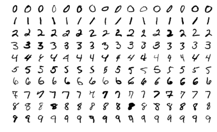
"Figure 1: A few digits from the MNIST dataset. Figure reference: en.wikipedia.org/wiki/MNIST_database.
\n", "\n",
"Figure 1: A few digits from the MNIST dataset. Figure reference: en.wikipedia.org/wiki/MNIST_database.
\n", "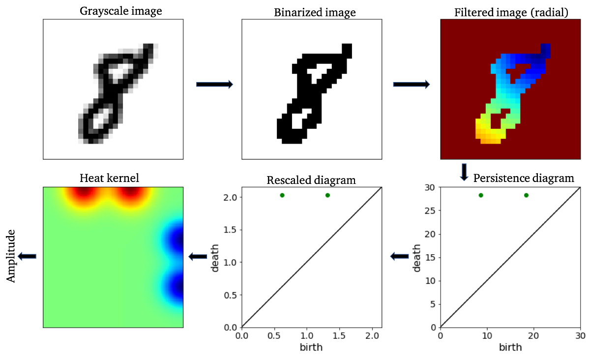 \n",
"
\n",
"Figure 2: An example of a topological feature extraction pipeline. Figure reference: arXiv:1910.08345.
\n", "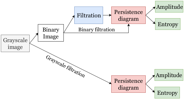 \n",
"
\n",
"Figure 3: A full-blown topological feature extraction pipeline
\n", " \n",
"
\n",
"