{
"cells": [
{
"cell_type": "markdown",
"source": [
"# Tutorial 23: Low-level API - Geometry"
],
"metadata": {}
},
{
"cell_type": "markdown",
"source": [
"In this tutorial, we will learn\n",
"\n",
" - How the `DiscreteModel` and its components work.\n",
" - How to extract topological information from a `GridTopology`.\n",
" - How to extract geometrical information from a `Grid`.\n",
" - How periodicity is handled in Gridap, and the difference between nodes and vertices.\n",
" - How to create a periodic model from scratch, use the example of a Mobius strip.\n",
"\n",
"## Required Packages"
],
"metadata": {}
},
{
"outputs": [],
"cell_type": "code",
"source": [
"using Gridap\n",
"using Gridap.Geometry, Gridap.ReferenceFEs, Gridap.Arrays\n",
"using Plots"
],
"metadata": {},
"execution_count": null
},
{
"cell_type": "markdown",
"source": [
"## Table of Contents\n",
"1. Utility Functions\n",
"2. The DiscreteModel Structure\n",
"3. Working with Topology\n",
"4. Geometric Mappings\n",
"5. High-order Grids\n",
"6. Periodicity in Gridap\n",
"\n",
"## 1. Utility Functions\n",
"We begin by defining helper functions that will be essential throughout this tutorial.\n",
"These functions help us visualize and work with our mesh structures."
],
"metadata": {}
},
{
"cell_type": "markdown",
"source": [
"Convert a CartesianDiscreteModel to an UnstructuredDiscreteModel for more generic handling"
],
"metadata": {}
},
{
"outputs": [],
"cell_type": "code",
"source": [
"function cartesian_model(args...; kwargs...)\n",
" UnstructuredDiscreteModel(CartesianDiscreteModel(args...; kwargs...))\n",
"end"
],
"metadata": {},
"execution_count": null
},
{
"cell_type": "markdown",
"source": [
"Visualization function to plot nodes with their IDs\n",
"Input: node_coords - Array of node coordinates\n",
" node_ids - Array of corresponding node IDs"
],
"metadata": {}
},
{
"outputs": [],
"cell_type": "code",
"source": [
"function plot_node_numbering(node_coords, node_ids)\n",
" x = map(c -> c[1], node_coords)\n",
" y = map(c -> c[2], node_coords)\n",
" a = text.(node_ids, halign=:left, valign=:bottom)\n",
" scatter(x, y, series_annotations = a, legend=false)\n",
" hline!(unique(x), linestyle=:dash, color=:grey)\n",
" vline!(unique(y), linestyle=:dash, color=:grey)\n",
"end"
],
"metadata": {},
"execution_count": null
},
{
"cell_type": "markdown",
"source": [
"Overloaded method to plot node numbering directly from a model\n",
"This function extracts the necessary information from the model and calls the base plotting function"
],
"metadata": {}
},
{
"outputs": [],
"cell_type": "code",
"source": [
"function plot_node_numbering(model)\n",
" D = num_cell_dims(model)\n",
" topo = get_grid_topology(model)\n",
" node_coords = Geometry.get_node_coordinates(model)\n",
" cell_node_ids = get_cell_node_ids(model)\n",
" cell_vertex_ids = Geometry.get_faces(topo, D, 0)\n",
"\n",
" node_to_vertex = zeros(Int, length(node_coords))\n",
" for (nodes,vertices) in zip(cell_node_ids, cell_vertex_ids)\n",
" node_to_vertex[nodes] .= vertices\n",
" end\n",
"\n",
" plot_node_numbering(node_coords, node_to_vertex)\n",
"end"
],
"metadata": {},
"execution_count": null
},
{
"cell_type": "markdown",
"source": [
"## 2. The DiscreteModel Structure\n",
"\n",
"The `DiscreteModel` in Gridap is a fundamental structure that represents a discretized\n",
"computational domain. It consists of three main components, each serving a specific purpose:\n",
"\n",
" - The `GridTopology`: Defines the connectivity of the mesh elements\n",
" * Stores how vertices, edges, faces, and cells are connected\n",
" * Enables neighbor queries and traversal of the mesh\n",
" * Pure topological information, no geometric data\n",
"\n",
" - The `Grid`: Contains the geometric information of the mesh\n",
" * Stores coordinates of mesh nodes\n",
" * Provides mappings between reference and physical elements\n",
" * Handles curved elements and high-order geometries\n",
"\n",
" - The `FaceLabeling`: Manages mesh labels and markers\n",
" * Identifies boundary regions\n",
" * Tags different material regions\n",
" * Essential for applying boundary conditions\n",
"\n",
"### Key Concept: Nodes vs. Vertices\n",
"\n",
"One of the most important distinctions in Gridap is between nodes and vertices:\n",
"\n",
" - **Vertices** (Topological entities):\n",
" * 0-dimensional entities in the `GridTopology`\n",
" * Define the connectivity of the mesh\n",
" * Used for neighbor queries and mesh traversal\n",
" * Number of vertices depends only on topology\n",
"\n",
" - **Nodes** (Geometric entities):\n",
" * Control points stored in the `Grid`\n",
" * Define the geometry of elements\n",
" * Used for interpolation and mapping\n",
" * Number of nodes depends on the geometric order\n",
"\n",
"While nodes and vertices often coincide in simple meshes, they differ in two important cases:\n",
"1. Periodic meshes: Where multiple nodes may correspond to the same vertex\n",
"2. High-order meshes: Where additional nodes are needed to represent curved geometries\n",
"\n",
"## 3. Working with Topology\n",
"\n",
"Let's explore how to extract and work with topological information. We'll start by creating\n",
"a simple 3x3 cartesian mesh:"
],
"metadata": {}
},
{
"outputs": [],
"cell_type": "code",
"source": [
"model = cartesian_model((0,1,0,1),(3,3))"
],
"metadata": {},
"execution_count": null
},
{
"cell_type": "markdown",
"source": [
"First, let's get the topology component and count the mesh entities:"
],
"metadata": {}
},
{
"outputs": [],
"cell_type": "code",
"source": [
"topo = get_grid_topology(model)\n",
"\n",
"n_vertices = num_faces(topo,0) # Number of vertices (0-dimensional entities)\n",
"n_edges = num_faces(topo,1) # Number of edges (1-dimensional entities)\n",
"n_cells = num_faces(topo,2) # Number of cells (2-dimensional entities)"
],
"metadata": {},
"execution_count": null
},
{
"cell_type": "markdown",
"source": [
"### Connectivity Queries\n",
"Gridap provides various methods to query the connectivity between different mesh entities.\n",
"Here are some common queries:"
],
"metadata": {}
},
{
"cell_type": "markdown",
"source": [
"Get vertices of each cell (cell → vertex connectivity)"
],
"metadata": {}
},
{
"outputs": [],
"cell_type": "code",
"source": [
"cell_to_vertices = get_faces(topo,2,0)"
],
"metadata": {},
"execution_count": null
},
{
"cell_type": "markdown",
"source": [
"Get edges of each cell (cell → edge connectivity)"
],
"metadata": {}
},
{
"outputs": [],
"cell_type": "code",
"source": [
"cell_to_edges = get_faces(topo,2,1)"
],
"metadata": {},
"execution_count": null
},
{
"cell_type": "markdown",
"source": [
"Get cells adjacent to each edge (edge → cell connectivity)"
],
"metadata": {}
},
{
"outputs": [],
"cell_type": "code",
"source": [
"edge_to_cells = get_faces(topo,1,2)"
],
"metadata": {},
"execution_count": null
},
{
"cell_type": "markdown",
"source": [
"Get vertices of each edge (edge → vertex connectivity)"
],
"metadata": {}
},
{
"outputs": [],
"cell_type": "code",
"source": [
"edge_to_vertices = get_faces(topo,1,0)"
],
"metadata": {},
"execution_count": null
},
{
"cell_type": "markdown",
"source": [
"### Advanced Connectivity: Finding Cell Neighbors\n",
"\n",
"Finding cells that share entities (like vertices or edges) requires more work.\n",
"A direct query for cell-to-cell connectivity returns an identity map:"
],
"metadata": {}
},
{
"outputs": [],
"cell_type": "code",
"source": [
"cell_to_cells = get_faces(topo,2,2) # Returns identity table"
],
"metadata": {},
"execution_count": null
},
{
"cell_type": "markdown",
"source": [
"To find actual cell neighbors, we need to traverse through lower-dimensional entities.\n",
"Here's a utility function that builds a face-to-face connectivity graph:"
],
"metadata": {}
},
{
"outputs": [],
"cell_type": "code",
"source": [
"function get_face_to_face_graph(topo,Df)\n",
" n_faces = num_faces(topo,Df)\n",
" face_to_vertices = get_faces(topo,Df,0) # Get vertices of each face\n",
" vertex_to_faces = get_faces(topo,0,Df) # Get faces incident to each vertex\n",
"\n",
" face_to_face = Vector{Vector{Int}}(undef,n_faces)\n",
" for face in 1:n_faces\n",
" nbors = Int[]\n",
" for vertex in face_to_vertices[face]\n",
" append!(nbors,vertex_to_faces[vertex]) # Add incident faces\n",
" end\n",
" face_to_face[face] = filter(!isequal(face),unique(nbors)) # Remove self-reference and duplicates\n",
" end\n",
"\n",
" return face_to_face\n",
"end"
],
"metadata": {},
"execution_count": null
},
{
"cell_type": "markdown",
"source": [
"Now we can find neighboring cells and edges:"
],
"metadata": {}
},
{
"outputs": [],
"cell_type": "code",
"source": [
"cell_to_cells = get_face_to_face_graph(topo,2) # Cells sharing vertices\n",
"edge_to_edges = get_face_to_face_graph(topo,1) # Edges sharing vertices"
],
"metadata": {},
"execution_count": null
},
{
"cell_type": "markdown",
"source": [
"## 4. Geometric Mappings\n",
"\n",
"The geometry of our mesh is defined by mappings from reference elements to physical space.\n",
"Let's explore how these mappings work in Gridap:"
],
"metadata": {}
},
{
"outputs": [],
"cell_type": "code",
"source": [
"grid = get_grid(model)"
],
"metadata": {},
"execution_count": null
},
{
"cell_type": "markdown",
"source": [
"First, we extract the basic geometric information:"
],
"metadata": {}
},
{
"outputs": [],
"cell_type": "code",
"source": [
"cell_map = get_cell_map(grid) # Mapping from reference to physical space\n",
"cell_to_nodes = get_cell_node_ids(grid) # Node IDs for each cell\n",
"node_coordinates = get_node_coordinates(grid) # Physical coordinates of nodes"
],
"metadata": {},
"execution_count": null
},
{
"cell_type": "markdown",
"source": [
"### Computing Cell-wise Node Coordinates\n",
"\n",
"There are two ways to get the coordinates of nodes for each cell:\n",
"\n",
"1. Using standard Julia mapping:"
],
"metadata": {}
},
{
"outputs": [],
"cell_type": "code",
"source": [
"cell_to_node_coords = map(nodes -> node_coordinates[nodes], cell_to_nodes)"
],
"metadata": {},
"execution_count": null
},
{
"cell_type": "markdown",
"source": [
"2. Using Gridap's lazy evaluation system (more efficient for large meshes):"
],
"metadata": {}
},
{
"outputs": [],
"cell_type": "code",
"source": [
"cell_to_node_coords = lazy_map(Broadcasting(Reindex(node_coordinates)),cell_to_nodes)"
],
"metadata": {},
"execution_count": null
},
{
"cell_type": "markdown",
"source": [
"### Geometric Mappings\n",
"\n",
"The mapping from reference to physical space is defined by cell-wise linear combination of:\n",
"1. Reference element shape functions (basis)\n",
"2. Physical node coordinates (coefficients)"
],
"metadata": {}
},
{
"outputs": [],
"cell_type": "code",
"source": [
"cell_reffes = get_cell_reffe(grid) # Get reference elements for each cell\n",
"cell_basis = lazy_map(get_shapefuns,cell_reffes) # Get basis functions\n",
"cell_map = lazy_map(linear_combination,cell_to_node_coords,cell_basis)"
],
"metadata": {},
"execution_count": null
},
{
"cell_type": "markdown",
"source": [
"## 5. High-order Grids\n",
"\n",
"High-order geometric representations are essential for accurately modeling curved boundaries\n",
"and complex geometries. Let's explore this by creating a curved mesh:\n",
"\n",
"### Example: Creating a Half-Cylinder\n",
"\n",
"First, we define a mapping that transforms our planar mesh into a half-cylinder:"
],
"metadata": {}
},
{
"outputs": [],
"cell_type": "code",
"source": [
"function F(x)\n",
" θ = x[1]*pi # Map x-coordinate to angle [0,π]\n",
" z = x[2] # Keep y-coordinate as height\n",
" VectorValue(cos(θ),sin(θ),z) # Convert to cylindrical coordinates\n",
"end"
],
"metadata": {},
"execution_count": null
},
{
"cell_type": "markdown",
"source": [
"Apply the mapping to our node coordinates:"
],
"metadata": {}
},
{
"outputs": [],
"cell_type": "code",
"source": [
"new_node_coordinates = map(F,node_coordinates)"
],
"metadata": {},
"execution_count": null
},
{
"cell_type": "markdown",
"source": [
"Create new cell mappings with the transformed coordinates:"
],
"metadata": {}
},
{
"outputs": [],
"cell_type": "code",
"source": [
"new_cell_to_node_coords = lazy_map(Broadcasting(Reindex(new_node_coordinates)),cell_to_nodes)\n",
"new_cell_map = lazy_map(linear_combination,new_cell_to_node_coords,cell_basis)"
],
"metadata": {},
"execution_count": null
},
{
"cell_type": "markdown",
"source": [
"Create a new grid with the transformed geometry:"
],
"metadata": {}
},
{
"outputs": [],
"cell_type": "code",
"source": [
"reffes, cell_types = compress_cell_data(cell_reffes)\n",
"new_grid = UnstructuredGrid(new_node_coordinates,cell_to_nodes,reffes,cell_types)"
],
"metadata": {},
"execution_count": null
},
{
"cell_type": "markdown",
"source": [
"Save for visualization:"
],
"metadata": {}
},
{
"outputs": [],
"cell_type": "code",
"source": [
"writevtk(new_grid,\"half_cylinder_linear\")"
],
"metadata": {},
"execution_count": null
},
{
"cell_type": "markdown",
"source": [
"If we visualize the result, we'll notice that despite applying a curved mapping,\n",
"our half-cylinder looks faceted. This is because we're still using linear elements\n",
"(straight edges) to approximate the curved geometry.\n",
"\n",
"### Solution: High-order Elements\n",
"\n",
"To accurately represent curved geometries, we need high-order elements:"
],
"metadata": {}
},
{
"cell_type": "markdown",
"source": [
"Create quadratic reference elements:"
],
"metadata": {}
},
{
"outputs": [],
"cell_type": "code",
"source": [
"order = 2 # Polynomial order\n",
"new_reffes = [LagrangianRefFE(Float64,QUAD,order)] # Quadratic quadrilateral elements\n",
"new_cell_reffes = expand_cell_data(new_reffes,cell_types)"
],
"metadata": {},
"execution_count": null
},
{
"cell_type": "markdown",
"source": [
"Create a finite element space to handle the high-order geometry:"
],
"metadata": {}
},
{
"outputs": [],
"cell_type": "code",
"source": [
"space = FESpace(model,new_cell_reffes)\n",
"new_cell_to_nodes = get_cell_dof_ids(space)"
],
"metadata": {},
"execution_count": null
},
{
"cell_type": "markdown",
"source": [
"Get the quadratic nodes in the reference element:"
],
"metadata": {}
},
{
"outputs": [],
"cell_type": "code",
"source": [
"cell_dofs = lazy_map(get_dof_basis,new_cell_reffes)\n",
"cell_basis = lazy_map(get_shapefuns,new_cell_reffes)\n",
"cell_to_ref_coordinates = lazy_map(get_nodes,cell_dofs)"
],
"metadata": {},
"execution_count": null
},
{
"cell_type": "markdown",
"source": [
"Map the reference nodes to the physical space:"
],
"metadata": {}
},
{
"outputs": [],
"cell_type": "code",
"source": [
"cell_to_phys_coordinates = lazy_map(evaluate,cell_map,cell_to_ref_coordinates)"
],
"metadata": {},
"execution_count": null
},
{
"cell_type": "markdown",
"source": [
"Create the high-order node coordinates:"
],
"metadata": {}
},
{
"outputs": [],
"cell_type": "code",
"source": [
"new_n_nodes = maximum(maximum,new_cell_to_nodes)\n",
"new_node_coordinates = zeros(VectorValue{2,Float64},new_n_nodes)\n",
"for (cell,nodes) in enumerate(new_cell_to_nodes)\n",
" for (i,node) in enumerate(nodes)\n",
" new_node_coordinates[node] = cell_to_phys_coordinates[cell][i]\n",
" end\n",
"end"
],
"metadata": {},
"execution_count": null
},
{
"cell_type": "markdown",
"source": [
"Apply our cylindrical mapping to the high-order nodes:"
],
"metadata": {}
},
{
"outputs": [],
"cell_type": "code",
"source": [
"new_node_coordinates = map(F,new_node_coordinates)"
],
"metadata": {},
"execution_count": null
},
{
"cell_type": "markdown",
"source": [
"Create the high-order grid:"
],
"metadata": {}
},
{
"outputs": [],
"cell_type": "code",
"source": [
"new_grid = UnstructuredGrid(new_node_coordinates,new_cell_to_nodes,new_reffes,cell_types)\n",
"writevtk(new_grid,\"half_cylinder_quadratic\")"
],
"metadata": {},
"execution_count": null
},
{
"cell_type": "markdown",
"source": [
"The resulting mesh now accurately represents the curved geometry of the half-cylinder,\n",
"with quadratic elements properly capturing the curvature (despite paraview still showing\n",
"a linear interpolation between the nodes)."
],
"metadata": {}
},
{
"cell_type": "markdown",
"source": [
"## 6. Periodicity in Gridap\n",
"\n",
"Periodic boundary conditions are essential in many applications, such as:\n",
"- Modeling crystalline materials\n",
"- Simulating fluid flow in periodic domains\n",
"- Analyzing electromagnetic wave propagation\n",
"\n",
"Gridap handles periodicity through a clever approach:\n",
"1. In the topology: Periodic vertices are \"glued\" together, creating a single topological entity\n",
"2. In the geometry: The corresponding nodes maintain their distinct physical positions\n",
"\n",
"This separation between topology and geometry allows us to:\n",
"- Maintain the correct geometric representation\n",
"- Automatically enforce periodic boundary conditions\n",
"- Avoid mesh distortion at periodic boundaries\n",
"\n",
"### Visualizing Periodicity\n",
"\n",
"Let's examine how periodicity affects the mesh structure through three examples:"
],
"metadata": {}
},
{
"cell_type": "markdown",
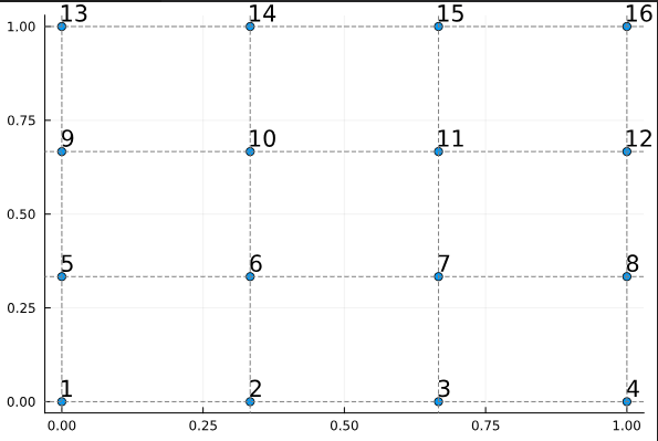
"source": [
"1. Standard non-periodic mesh:"
],
"metadata": {}
},
{
"outputs": [],
"cell_type": "code",
"source": [
"model = cartesian_model((0,1,0,1),(3,3))\n",
"plot_node_numbering(model)"
],
"metadata": {},
"execution_count": null
},
{
"cell_type": "markdown",
"source": [
""
],
"metadata": {}
},
{
"cell_type": "markdown",
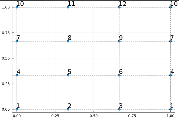
"source": [
"2. Mesh with periodicity in x-direction:"
],
"metadata": {}
},
{
"outputs": [],
"cell_type": "code",
"source": [
"model = cartesian_model((0,1,0,1),(3,3),isperiodic=(true,false))\n",
"plot_node_numbering(model)"
],
"metadata": {},
"execution_count": null
},
{
"cell_type": "markdown",
"source": [
""
],
"metadata": {}
},
{
"cell_type": "markdown",
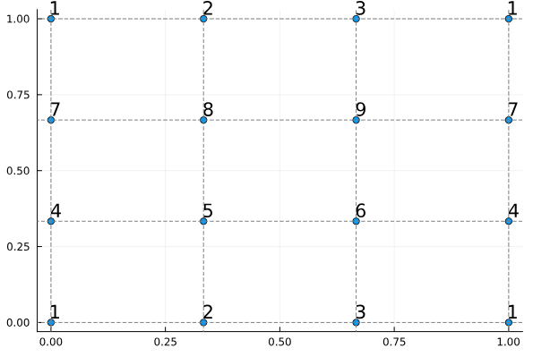
"source": [
"3. Mesh with periodicity in both directions:"
],
"metadata": {}
},
{
"outputs": [],
"cell_type": "code",
"source": [
"model = cartesian_model((0,1,0,1),(3,3),isperiodic=(true,true))\n",
"plot_node_numbering(model)"
],
"metadata": {},
"execution_count": null
},
{
"cell_type": "markdown",
"source": [
""
],
"metadata": {}
},
{
"cell_type": "markdown",
"source": [
"Notice how the vertex numbers (displayed at node positions) show the topological\n",
"connectivity, while the nodes remain at their physical positions.\n",
"\n",
"### Creating a Möbius Strip\n",
"\n",
"We'll create it by:\n",
"1. Starting with a rectangular mesh\n",
"2. Making it periodic in one direction\n",
"3. Adding a twist before connecting the ends\n",
"\n",
"#### Step 1: Create Base Mesh\n",
"\n",
"Start with a 3x3 cartesian mesh:"
],
"metadata": {}
},
{
"outputs": [],
"cell_type": "code",
"source": [
"nc = (3,3) # Number of cells in each direction\n",
"model = cartesian_model((0,1,0,1),nc)"
],
"metadata": {},
"execution_count": null
},
{
"cell_type": "markdown",
"source": [
"Extract geometric and topological information:"
],
"metadata": {}
},
{
"outputs": [],
"cell_type": "code",
"source": [
"node_coords = get_node_coordinates(model) # Physical positions\n",
"cell_node_ids = get_cell_node_ids(model) # Node connectivity\n",
"cell_type = get_cell_type(model) # Element type\n",
"reffes = get_reffes(model) # Reference elements"
],
"metadata": {},
"execution_count": null
},
{
"cell_type": "markdown",
"source": [
"#### Step 2: Create Periodic Topology\n",
"\n",
"To create the Möbius strip, we need to:\n",
"1. Identify vertices to be connected\n",
"2. Reverse one edge to create the twist\n",
"3. Ensure proper connectivity"
],
"metadata": {}
},
{
"cell_type": "markdown",
"source": [
"Create initial vertex numbering:"
],
"metadata": {}
},
{
"outputs": [],
"cell_type": "code",
"source": [
"np = nc .+ 1 # Number of points in each direction\n",
"mobius_ids = collect(LinearIndices(np))"
],
"metadata": {},
"execution_count": null
},
{
"cell_type": "markdown",
"source": [
"Create the twist by reversing the last row:"
],
"metadata": {}
},
{
"outputs": [],
"cell_type": "code",
"source": [
"mobius_ids[end,:] = reverse(mobius_ids[1,:])"
],
"metadata": {},
"execution_count": null
},
{
"cell_type": "markdown",
"source": [
"Map cell nodes to the new vertex numbering:"
],
"metadata": {}
},
{
"outputs": [],
"cell_type": "code",
"source": [
"cell_vertex_ids = map(nodes -> mobius_ids[nodes], cell_node_ids)"
],
"metadata": {},
"execution_count": null
},
{
"cell_type": "markdown",
"source": [
"#### Step 3: Clean Up Vertex Numbering\n",
"\n",
"The new vertex IDs aren't contiguous (some numbers are duplicated due to periodicity).\n",
"We need to create a clean mapping:"
],
"metadata": {}
},
{
"cell_type": "markdown",
"source": [
"Find unique vertices and create bidirectional mappings:"
],
"metadata": {}
},
{
"outputs": [],
"cell_type": "code",
"source": [
"vertex_to_node = unique(vcat(cell_vertex_ids...))\n",
"node_to_vertex = find_inverse_index_map(vertex_to_node)"
],
"metadata": {},
"execution_count": null
},
{
"cell_type": "markdown",
"source": [
"Renumber vertices to be contiguous:"
],
"metadata": {}
},
{
"outputs": [],
"cell_type": "code",
"source": [
"cell_vertex_ids = map(nodes -> node_to_vertex[nodes], cell_vertex_ids)"
],
"metadata": {},
"execution_count": null
},
{
"cell_type": "markdown",
"source": [
"Convert to the Table format required by Gridap:"
],
"metadata": {}
},
{
"outputs": [],
"cell_type": "code",
"source": [
"cell_vertex_ids = Table(cell_vertex_ids)"
],
"metadata": {},
"execution_count": null
},
{
"cell_type": "markdown",
"source": [
"Get coordinates for the vertices:"
],
"metadata": {}
},
{
"outputs": [],
"cell_type": "code",
"source": [
"vertex_coords = node_coords[vertex_to_node]\n",
"polytopes = map(get_polytope,reffes)"
],
"metadata": {},
"execution_count": null
},
{
"cell_type": "markdown",
"source": [
"#### Step 4: Create the Model\n",
"\n",
"Now we can create our Möbius strip model:"
],
"metadata": {}
},
{
"cell_type": "markdown",
"source": [
"Create topology with periodic connections:"
],
"metadata": {}
},
{
"outputs": [],
"cell_type": "code",
"source": [
"topo = UnstructuredGridTopology(\n",
" vertex_coords, cell_vertex_ids, cell_type, polytopes\n",
")"
],
"metadata": {},
"execution_count": null
},
{
"cell_type": "markdown",
"source": [
"Create grid (geometry remains unchanged):"
],
"metadata": {}
},
{
"outputs": [],
"cell_type": "code",
"source": [
"grid = UnstructuredGrid(\n",
" node_coords, cell_node_ids, reffes, cell_type\n",
")"
],
"metadata": {},
"execution_count": null
},
{
"cell_type": "markdown",
"source": [
"Add basic face labels:"
],
"metadata": {}
},
{
"outputs": [],
"cell_type": "code",
"source": [
"labels = FaceLabeling(topo)"
],
"metadata": {},
"execution_count": null
},
{
"cell_type": "markdown",
"source": [
"Combine into final model:"
],
"metadata": {}
},
{
"outputs": [],
"cell_type": "code",
"source": [
"mobius = UnstructuredDiscreteModel(grid,topo,labels)"
],
"metadata": {},
"execution_count": null
},
{
"cell_type": "markdown",
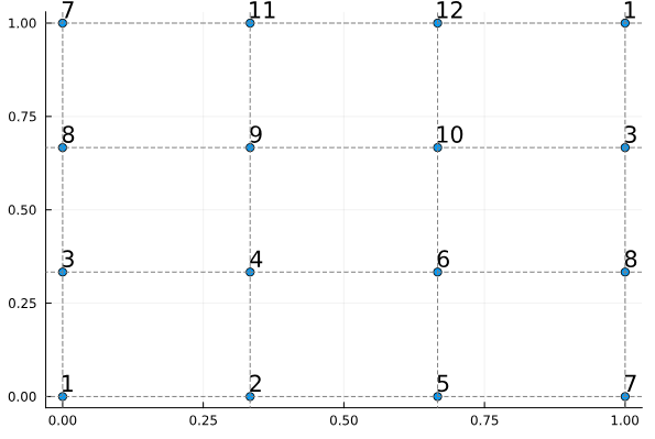
"source": [
"Visualize the vertex numbering:"
],
"metadata": {}
},
{
"outputs": [],
"cell_type": "code",
"source": [
"plot_node_numbering(mobius)"
],
"metadata": {},
"execution_count": null
},
{
"cell_type": "markdown",
"source": [
""
],
"metadata": {}
},
{
"cell_type": "markdown",
"source": [
"---\n",
"\n",
"*This notebook was generated using [Literate.jl](https://github.com/fredrikekre/Literate.jl).*"
],
"metadata": {}
}
],
"nbformat_minor": 3,
"metadata": {
"language_info": {
"file_extension": ".jl",
"mimetype": "application/julia",
"name": "julia",
"version": "1.10.8"
},
"kernelspec": {
"name": "julia-1.10",
"display_name": "Julia 1.10.8",
"language": "julia"
}
},
"nbformat": 4
}