# gdalio

[](https://github.com/hypertidy/gdalio/actions)
The goal of gdalio is to read data direct with GDAL warp, with a simple
configuration - specify the *target grid* once. This saves us from a lot
of complication, juggling of formats, objects, and extra code.
We have these functions to easily read raster data via the GDAL warp
library:
- `gdalio_data()` read data directly from a *data source name*
i.e. file path, url, or database connection
- `gdalio_set_default_grid()` specify a grid (extent, dimension,
projection) to use for all subsequent operations
- `gdalio_get_default_grid()` get the grid currently in use
- `vrt()` simple function (not actually VRT, but doing similar in a
limited way) to *augment* data sources that have missing or
incorrect *extent* or *projection* metadata
- `gdalio_matrix()`, `gdalio_array()`, and `gdalio_graphics()` which
reformat the data into commonly used R types for images
- `gdalio_data_hex()`, `gdalio_data_rgb()` special cases of
gdalio_data() to read 3 or 4 bands, convert to text hex codes
- `gdalio_local_grid()` a helper to create a local projected region
around a longlat (optional width extent, dimension, projection
family)
- `gdalio_format_source()` a helper to *return the file path* to
source code, to define formatters for spatial package types (raster,
stars, terra, spatstat).
In this readme we illustrate the use of these from some online and local
raster data sources, and provide helpers for reading into particular
formats used in R (base matrix, raster package, stars package, spatstat
package, terra package).
## Installation
You can install gdalio with:
``` r
#install.packages("remotes")
## currently need this branch to avoid dev problems in vapour
remotes::install_github("hypertidy/vapour@stable-2022")
remotes::install_github("hypertidy/gdalio")
```
## Target grid specification
Key is having a *target grid*, we nominate it upfront and then any data
we request from GDAL will *fill that grid* by GDAL’s warp magic.
A *grid* is an abstract description of an *image* data set:
- extent `(xmin, xmax, ymin, ymax)` in some coordinate system
- dimension (number of columns, number of rows)
- projection - the actual coordinate system
Often we have an actual object in some format that records this
information, but this can be much simpler by working with just 6 numbers
and one character string.
## Example
This works best for data you have access to locally, and in the simplest
case you could use gdalio like this, but more nuanced use requires some
effort to define the structure of the output data (which we explore
below).
``` r
library(gdalio)
vals <- gdal_data("myhugefile.tif")
```
For a real example we use a file that’s on the internet and requires a
little extra prep.
A sea surface temperature data set, we need GDAL’s subdataset syntax for
a file at a URL and *augment* our file address with what we know is the
projection of the data.
``` r
library(gdalio)
## online data, daily ocean temperature surface product, one layer in longlat 0.25 degree res
f <- vrt('NETCDF:"/vsicurl/https://www.ncei.noaa.gov/data/sea-surface-temperature-optimum-interpolation/v2.1/access/avhrr/201809/oisst-avhrr-v02r01.20180929.nc":sst',
projection = "+proj=longlat +datum=WGS84")
```
``` r
## we set up a grid (this is a *raster* in abstraction)
grid0 <- list(extent = c(-1e6, 1e6, -5e5, 5e5 ),
dimension = c(512, 256),
projection = "+proj=laea +lon_0=147 +lat_0=-42")
gdalio_set_default_grid(grid0)
```
And now start reading data.
``` r
## then we get GDAL to get a value for every pixel in our grid
pix <- gdalio_data(f)
## we have a list vector for each band (just one here)
plot(pix[[1]], pch = ".")
```
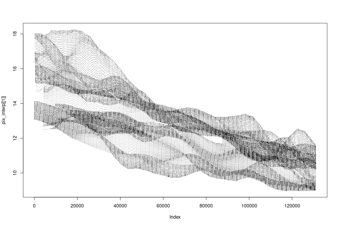
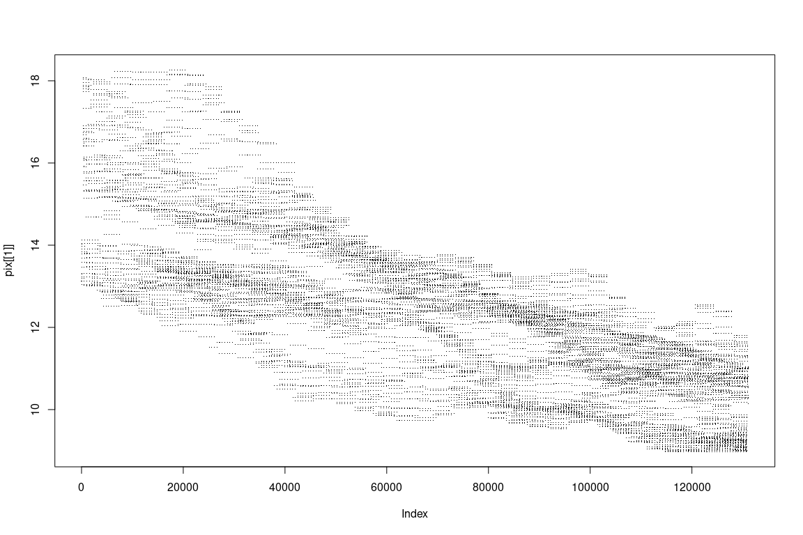 Those look a little simplified (it’s because we are asking for quite
high resolution from a low resolution source). So let’s use a different
*resampling* algorithm (default is nearest neighbour, no interpolation).
``` r
pix_interp <- gdalio_data(f, resample = "bilinear")
## use resampling we get quite a different result
plot(pix_interp[[1]], pch = ".")
```
Those look a little simplified (it’s because we are asking for quite
high resolution from a low resolution source). So let’s use a different
*resampling* algorithm (default is nearest neighbour, no interpolation).
``` r
pix_interp <- gdalio_data(f, resample = "bilinear")
## use resampling we get quite a different result
plot(pix_interp[[1]], pch = ".")
```
 Normally of course we want a bit more convenience, and actually fill a
format in R or some package that has spatial types. So we define those
helpers here.
## Raster formats
This function is equivalent to a number of others defined just below, to
format the data into objects used by various packages.
``` r
## simple list format used by graphics::image() - we can only handle one band/layer
gdalio_base <- function(dsn, ...) {
v <- gdalio_data(dsn, ...)
g <- gdalio_get_default_grid()
list(x = seq(g$extent[1], g$extent[2], length.out = g$dimension[1]),
y = seq(g$extent[3], g$extent[4], length.out = g$dimension[2]),
z = matrix(v[[1]], g$dimension[1])[, g$dimension[2]:1])
}
```
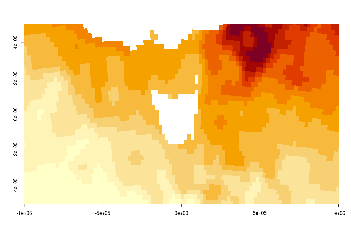
R for a long time had this powerful list(x,y,z) format for `image()`:
``` r
xyz <- gdalio_base(f)
image(xyz)
```
Normally of course we want a bit more convenience, and actually fill a
format in R or some package that has spatial types. So we define those
helpers here.
## Raster formats
This function is equivalent to a number of others defined just below, to
format the data into objects used by various packages.
``` r
## simple list format used by graphics::image() - we can only handle one band/layer
gdalio_base <- function(dsn, ...) {
v <- gdalio_data(dsn, ...)
g <- gdalio_get_default_grid()
list(x = seq(g$extent[1], g$extent[2], length.out = g$dimension[1]),
y = seq(g$extent[3], g$extent[4], length.out = g$dimension[2]),
z = matrix(v[[1]], g$dimension[1])[, g$dimension[2]:1])
}
```
R for a long time had this powerful list(x,y,z) format for `image()`:
``` r
xyz <- gdalio_base(f)
image(xyz)
```
 There are now several different formats used by various packages that
are equivalent. At root they specify *extent*, *dimension*, *projection*
the core concepts of our *target grid* (the less specialized ones ignore
the projection). Some of these kinds of functions require those
format-specific packages, but they are easy enough to write so we list
these here as examples.
There are functions `gdalio_matrix()`, `gdalio_array()`, and
`gdalio_graphics()` in this package that put the data into the native R
image form.
``` r
## {spatstat.geom}
gdalio_im <- function(dsn, ..., band_output_type = "numeric") {
v <- gdalio_data(dsn, ..., band_output_type = band_output_type)
g <- gdalio_get_default_grid()
## can we have a list of im?
if (length(v) > 1) message("only returning one image layer im, for now")
m <- matrix(v[[1]], g$dimension[1])
spatstat.geom::im(t(m[,ncol(m):1]), xrange = g$extent[1:2], yrange = g$extent[3:4])
}
## {raster}
gdalio_raster <-
function(dsn, ..., band_output_type = "numeric") {
v <- gdalio_data(dsn, ..., band_output_type = band_output_type)
g <- gdalio_get_default_grid()
r <- raster::raster(raster::extent(g$extent), nrows = g$dimension[2], ncols = g$dimension[1], crs = g$projection)
if (length(v) > 1) {
r <- raster::brick(replicate(length(v), r, simplify = FALSE))
}
raster::setValues(r, do.call(cbind, v))
}
## {terra}
gdalio_terra <- function(dsn, ..., band_output_type = "numeric") {
v <- gdalio_data(dsn, ..., band_output_type = band_output_type)
g <- gdalio_get_default_grid()
r <- terra::rast(terra::ext(g$extent), nrows = g$dimension[2], ncols = g$dimension[1], crs = g$projection)
if (length(v) > 1) terra::nlyr(r) <- length(v)
terra::setValues(r, do.call(cbind, v))
}
## {stars}
gdalio_stars <- function(dsn, ..., band_output_type = "numeric") {
v <- gdalio_data(dsn, ..., band_output_type = band_output_type)
g <- gdalio_get_default_grid()
aa <- array(unlist(v, use.names = FALSE), c(g$dimension[1], g$dimension[2], length(v)))#[,g$dimension[2]:1, , drop = FALSE]
if (length(v) == 1) aa <- aa[,,1, drop = TRUE]
r <- stars::st_as_stars(sf::st_bbox(c(xmin = g$extent[1], ymin = g$extent[3], xmax = g$extent[2], ymax = g$extent[4])),
nx = g$dimension[1], ny = g$dimension[2], values = aa)
r <- sf::st_set_crs(r, g$projection)
r
}
```
To obtain all of those functions you can do, but note the entire
dependency requirement includes at least raster, stars, spatstat.geom,
terra, so simply use the definitions as needed.
``` r
source(gdalio_format_source())
```
Note that for each format there is nothing of consequence that is
different, from the perspective of gdalio they all take the same set of
pixel values, there are just tiny differences in how the extent and
projection metadata are handled, and in storage orientation for the data
itself.
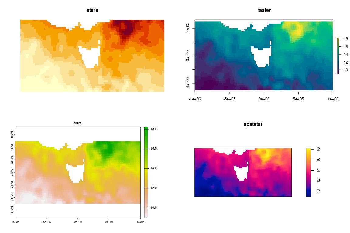
To prove the point we now read the same data but into our format of
choice. We are *re-reading* data here (it all exists in `pix` above, but
you get the idea).
``` r
op <- par(mfrow = c(2, 2))
#plot(matrix(g$extent, ncol = 2), type = "n", asp = 1, xlab = "x", ylab = "y", main = "stars")
image(gdalio_stars(f), main = "stars")
raster::plot(gdalio_raster(f), col = hcl.colors(26), main = "raster")
terra::plot(gdalio_terra(f), main = "terra")
plot(gdalio_im(f), main = "\nspatstat")
```
There are now several different formats used by various packages that
are equivalent. At root they specify *extent*, *dimension*, *projection*
the core concepts of our *target grid* (the less specialized ones ignore
the projection). Some of these kinds of functions require those
format-specific packages, but they are easy enough to write so we list
these here as examples.
There are functions `gdalio_matrix()`, `gdalio_array()`, and
`gdalio_graphics()` in this package that put the data into the native R
image form.
``` r
## {spatstat.geom}
gdalio_im <- function(dsn, ..., band_output_type = "numeric") {
v <- gdalio_data(dsn, ..., band_output_type = band_output_type)
g <- gdalio_get_default_grid()
## can we have a list of im?
if (length(v) > 1) message("only returning one image layer im, for now")
m <- matrix(v[[1]], g$dimension[1])
spatstat.geom::im(t(m[,ncol(m):1]), xrange = g$extent[1:2], yrange = g$extent[3:4])
}
## {raster}
gdalio_raster <-
function(dsn, ..., band_output_type = "numeric") {
v <- gdalio_data(dsn, ..., band_output_type = band_output_type)
g <- gdalio_get_default_grid()
r <- raster::raster(raster::extent(g$extent), nrows = g$dimension[2], ncols = g$dimension[1], crs = g$projection)
if (length(v) > 1) {
r <- raster::brick(replicate(length(v), r, simplify = FALSE))
}
raster::setValues(r, do.call(cbind, v))
}
## {terra}
gdalio_terra <- function(dsn, ..., band_output_type = "numeric") {
v <- gdalio_data(dsn, ..., band_output_type = band_output_type)
g <- gdalio_get_default_grid()
r <- terra::rast(terra::ext(g$extent), nrows = g$dimension[2], ncols = g$dimension[1], crs = g$projection)
if (length(v) > 1) terra::nlyr(r) <- length(v)
terra::setValues(r, do.call(cbind, v))
}
## {stars}
gdalio_stars <- function(dsn, ..., band_output_type = "numeric") {
v <- gdalio_data(dsn, ..., band_output_type = band_output_type)
g <- gdalio_get_default_grid()
aa <- array(unlist(v, use.names = FALSE), c(g$dimension[1], g$dimension[2], length(v)))#[,g$dimension[2]:1, , drop = FALSE]
if (length(v) == 1) aa <- aa[,,1, drop = TRUE]
r <- stars::st_as_stars(sf::st_bbox(c(xmin = g$extent[1], ymin = g$extent[3], xmax = g$extent[2], ymax = g$extent[4])),
nx = g$dimension[1], ny = g$dimension[2], values = aa)
r <- sf::st_set_crs(r, g$projection)
r
}
```
To obtain all of those functions you can do, but note the entire
dependency requirement includes at least raster, stars, spatstat.geom,
terra, so simply use the definitions as needed.
``` r
source(gdalio_format_source())
```
Note that for each format there is nothing of consequence that is
different, from the perspective of gdalio they all take the same set of
pixel values, there are just tiny differences in how the extent and
projection metadata are handled, and in storage orientation for the data
itself.
To prove the point we now read the same data but into our format of
choice. We are *re-reading* data here (it all exists in `pix` above, but
you get the idea).
``` r
op <- par(mfrow = c(2, 2))
#plot(matrix(g$extent, ncol = 2), type = "n", asp = 1, xlab = "x", ylab = "y", main = "stars")
image(gdalio_stars(f), main = "stars")
raster::plot(gdalio_raster(f), col = hcl.colors(26), main = "raster")
terra::plot(gdalio_terra(f), main = "terra")
plot(gdalio_im(f), main = "\nspatstat")
```
 ``` r
par(op)
```
### Resampling algorithm
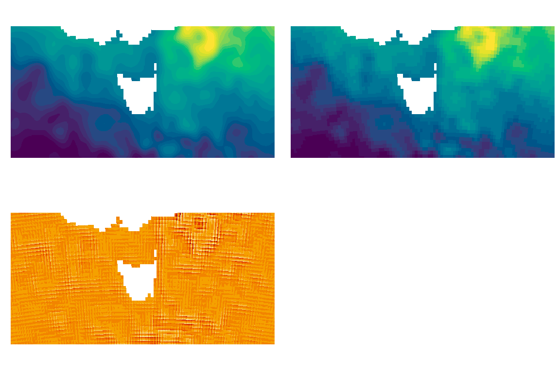
In the same way, we can also use different methods of resampling and
easily see the effect.
``` r
op <- par(mfrow = c(2, 2), mar = par("mar")/3)
image(cs <- gdalio_stars(f, resample = "cubicspline"), col = hcl.colors(26))
image(lz <- gdalio_stars(f, resample = "near"), col = hcl.colors(26))
image(cs - lz)
par(op)
```
``` r
par(op)
```
### Resampling algorithm
In the same way, we can also use different methods of resampling and
easily see the effect.
``` r
op <- par(mfrow = c(2, 2), mar = par("mar")/3)
image(cs <- gdalio_stars(f, resample = "cubicspline"), col = hcl.colors(26))
image(lz <- gdalio_stars(f, resample = "near"), col = hcl.colors(26))
image(cs - lz)
par(op)
```
 ## Imagery
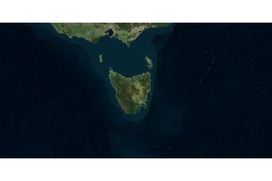
This works as well for online image sources (like photos or street
maps).
``` r
virtualearth_imagery <- tempfile(fileext = ".xml")
writeLines('
http://a${server_num}.ortho.tiles.virtualearth.net/tiles/a${quadkey}.jpeg?g=90
4
', virtualearth_imagery)
img <- gdalio_raster(virtualearth_imagery, bands = 1:3)
raster::plotRGB(img)
```
## Imagery
This works as well for online image sources (like photos or street
maps).
``` r
virtualearth_imagery <- tempfile(fileext = ".xml")
writeLines('
http://a${server_num}.ortho.tiles.virtualearth.net/tiles/a${quadkey}.jpeg?g=90
4
', virtualearth_imagery)
img <- gdalio_raster(virtualearth_imagery, bands = 1:3)
raster::plotRGB(img)
```
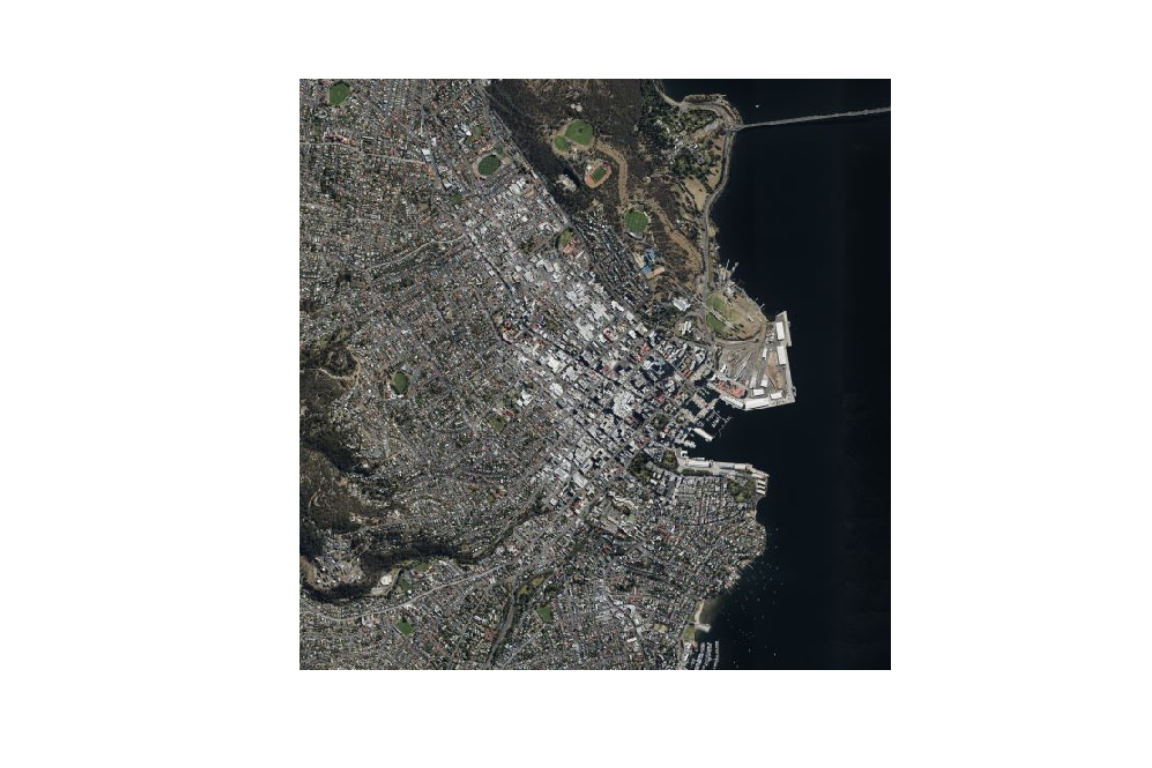
 ``` r
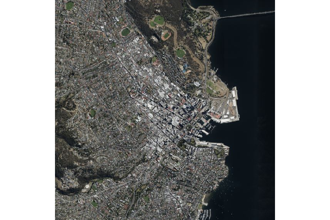
## let's really zoom in on somewhere cool
grid1 <- list(extent = c(-1, 1, -1, 1) * 2e3,
dimension = c(512, 512),
projection = "+proj=laea +lon_0=147.325 +lat_0=-42.880556")
gdalio_set_default_grid(grid1)
img <- gdalio_raster(virtualearth_imagery, bands = 1:3)
raster::plotRGB(img)
```
``` r
## let's really zoom in on somewhere cool
grid1 <- list(extent = c(-1, 1, -1, 1) * 2e3,
dimension = c(512, 512),
projection = "+proj=laea +lon_0=147.325 +lat_0=-42.880556")
gdalio_set_default_grid(grid1)
img <- gdalio_raster(virtualearth_imagery, bands = 1:3)
raster::plotRGB(img)
```
 To obtain the raw data values we can use `gdalio_data_rgb()` or
`gdalio_data_hex()` without specifying the number of bands, but these
are a little experimental for now.
``` r
rgbvals <- gdalio_data_rgb(virtualearth_imagery)
hexvals <- gdalio_data_hex(virtualearth_imagery)
```
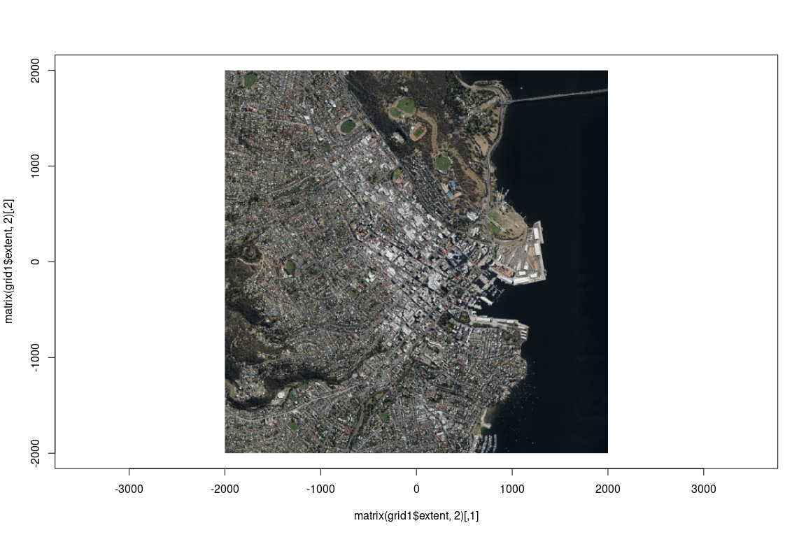
We can use this to drive R’s own raster type, the
`grDevices::as.raster()` array.
``` r
arr <- gdalio_graphics(virtualearth_imagery)
grid1 <- gdalio_get_default_grid()
plot(matrix(grid1$extent, 2), type = "n", asp = 1)
graphics::rasterImage(arr, grid1$extent[1], grid1$extent[3], grid1$extent[2], grid1$extent[4])
```
To obtain the raw data values we can use `gdalio_data_rgb()` or
`gdalio_data_hex()` without specifying the number of bands, but these
are a little experimental for now.
``` r
rgbvals <- gdalio_data_rgb(virtualearth_imagery)
hexvals <- gdalio_data_hex(virtualearth_imagery)
```
We can use this to drive R’s own raster type, the
`grDevices::as.raster()` array.
``` r
arr <- gdalio_graphics(virtualearth_imagery)
grid1 <- gdalio_get_default_grid()
plot(matrix(grid1$extent, 2), type = "n", asp = 1)
graphics::rasterImage(arr, grid1$extent[1], grid1$extent[3], grid1$extent[2], grid1$extent[4])
```
 Using R itself we can `plot()` but we must use a different idiom for the
extent.
*Don’t use `plot(arr, xlim = ,ylim = )` it does not work as claimed we
can only get sensible extents at R version 4.1.0 with `rasterImage()`.*
``` r
plot(arr)
```
Using R itself we can `plot()` but we must use a different idiom for the
extent.
*Don’t use `plot(arr, xlim = ,ylim = )` it does not work as claimed we
can only get sensible extents at R version 4.1.0 with `rasterImage()`.*
``` r
plot(arr)
```
 ``` r
par("usr")
#> [1] -191.1688 703.1688 0.0000 512.0000
```
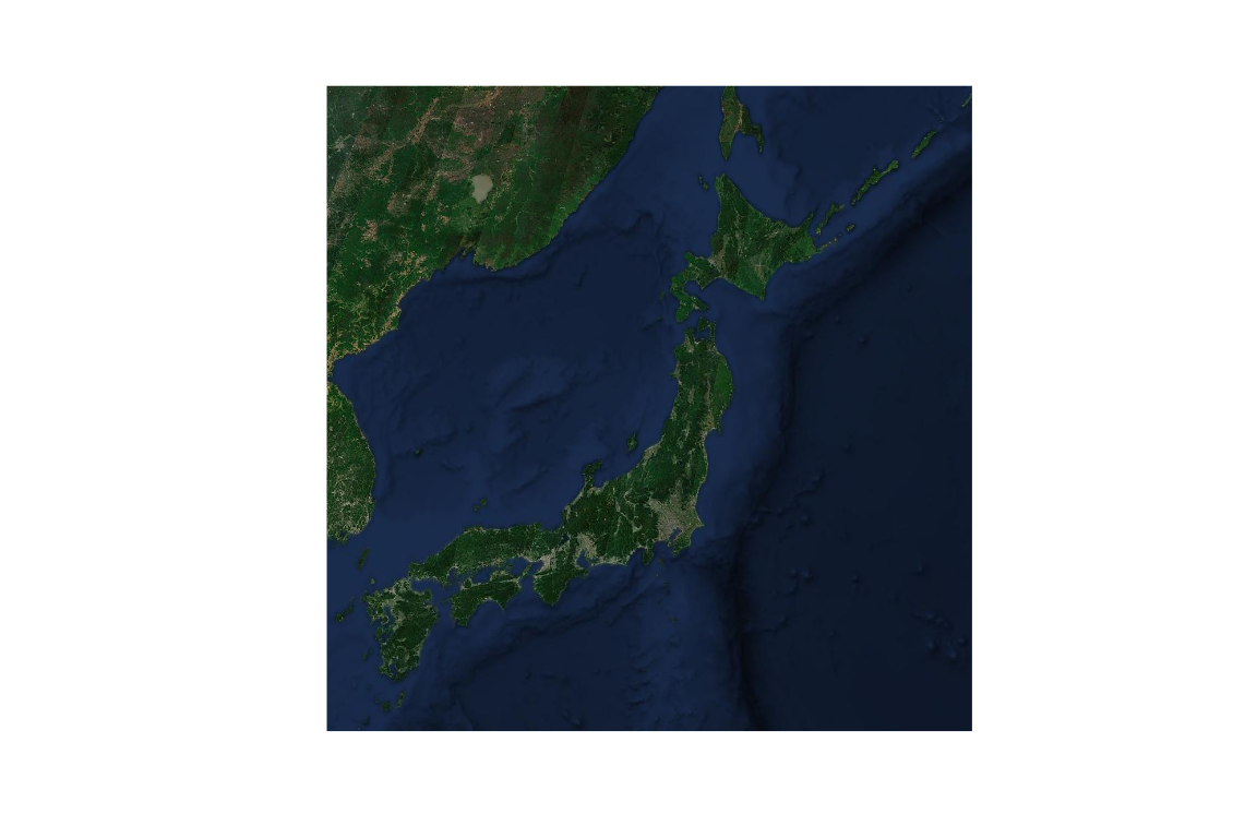
Another great example off twitter.
``` r
u <- "WMS:https://tiles.maps.eox.at/?SERVICE=WMS&VERSION=1.1.1&REQUEST=GetMap&LAYERS=s2cloudless-2019&SRS=EPSG:4326&BBOX=-180.000000,-90.000000,180.000000,90.000000&FORMAT=image/png&TILESIZE=256&OVERVIEWCOUNT=17&MINRESOLUTION=0.0000053644180298&TILED=true"
library(gdalio) ## https://github.com/hypertidy/gdalio
gdalio_set_default_grid(list(extent = c(-1, 1, -1, 1) * 1e6,
dimension = c(1024, 1024),
projection = "+proj=laea +lon_0=139 +lat_0=39"))
x <- gdalio_graphics(u)
plot(x)
```
``` r
par("usr")
#> [1] -191.1688 703.1688 0.0000 512.0000
```
Another great example off twitter.
``` r
u <- "WMS:https://tiles.maps.eox.at/?SERVICE=WMS&VERSION=1.1.1&REQUEST=GetMap&LAYERS=s2cloudless-2019&SRS=EPSG:4326&BBOX=-180.000000,-90.000000,180.000000,90.000000&FORMAT=image/png&TILESIZE=256&OVERVIEWCOUNT=17&MINRESOLUTION=0.0000053644180298&TILED=true"
library(gdalio) ## https://github.com/hypertidy/gdalio
gdalio_set_default_grid(list(extent = c(-1, 1, -1, 1) * 1e6,
dimension = c(1024, 1024),
projection = "+proj=laea +lon_0=139 +lat_0=39"))
x <- gdalio_graphics(u)
plot(x)
```
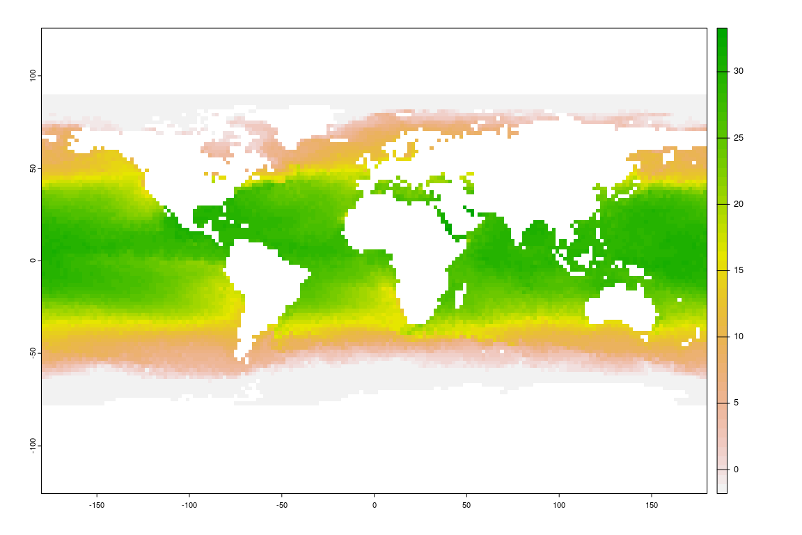
 ## Default grid (there is one)
Say we don’t set a grid at all, just go a default. Currently gdalio has
a default for an entire world longlat grid. This means we can read from
any source and we’ll get something (though we might not see anything if
the source is a tiny region).
``` r
gdalio_set_default_grid()
terra::plot(gdalio_terra(f))
```
## Default grid (there is one)
Say we don’t set a grid at all, just go a default. Currently gdalio has
a default for an entire world longlat grid. This means we can read from
any source and we’ll get something (though we might not see anything if
the source is a tiny region).
``` r
gdalio_set_default_grid()
terra::plot(gdalio_terra(f))
```
 ## Miscellaneous
Some sources, files in spData, image servers, etc.
``` r
elevation.tiles.prod <- tempfile(fileext = ".xml")
writeLines('
https://s3.amazonaws.com/elevation-tiles-prod/geotiff/${z}/${x}/${y}.tif
-20037508.34
20037508.34
20037508.34
-20037508.34
14
1
1
top
EPSG:3857
512
512
1
Int16
403,404
-32768
', elevation.tiles.prod)
## we'll use this as a grid specification, not the actual data for anything
sfiles <- list.files(system.file("raster", package = "spDataLarge", mustWork = TRUE), full.names = TRUE)
## we don't take raster objects, just the spec: extent, dim, projection
ri <- vapour::vapour_raster_info(sfiles[1])
gdalio_set_default_grid(list(extent = ri$extent,
dimension = ri$dimXY,
projection = ri$projection))
s <- gdalio_stars(elevation.tiles.prod)
library(stars); plot(s)
#> Loading required package: abind
#> Loading required package: sf
#> Linking to GEOS 3.10.1, GDAL 3.4.0, PROJ 8.2.0; sf_use_s2() is TRUE
```
## Miscellaneous
Some sources, files in spData, image servers, etc.
``` r
elevation.tiles.prod <- tempfile(fileext = ".xml")
writeLines('
https://s3.amazonaws.com/elevation-tiles-prod/geotiff/${z}/${x}/${y}.tif
-20037508.34
20037508.34
20037508.34
-20037508.34
14
1
1
top
EPSG:3857
512
512
1
Int16
403,404
-32768
', elevation.tiles.prod)
## we'll use this as a grid specification, not the actual data for anything
sfiles <- list.files(system.file("raster", package = "spDataLarge", mustWork = TRUE), full.names = TRUE)
## we don't take raster objects, just the spec: extent, dim, projection
ri <- vapour::vapour_raster_info(sfiles[1])
gdalio_set_default_grid(list(extent = ri$extent,
dimension = ri$dimXY,
projection = ri$projection))
s <- gdalio_stars(elevation.tiles.prod)
library(stars); plot(s)
#> Loading required package: abind
#> Loading required package: sf
#> Linking to GEOS 3.10.1, GDAL 3.4.0, PROJ 8.2.0; sf_use_s2() is TRUE
```
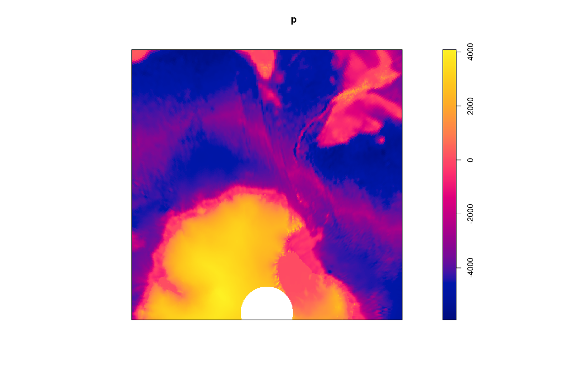
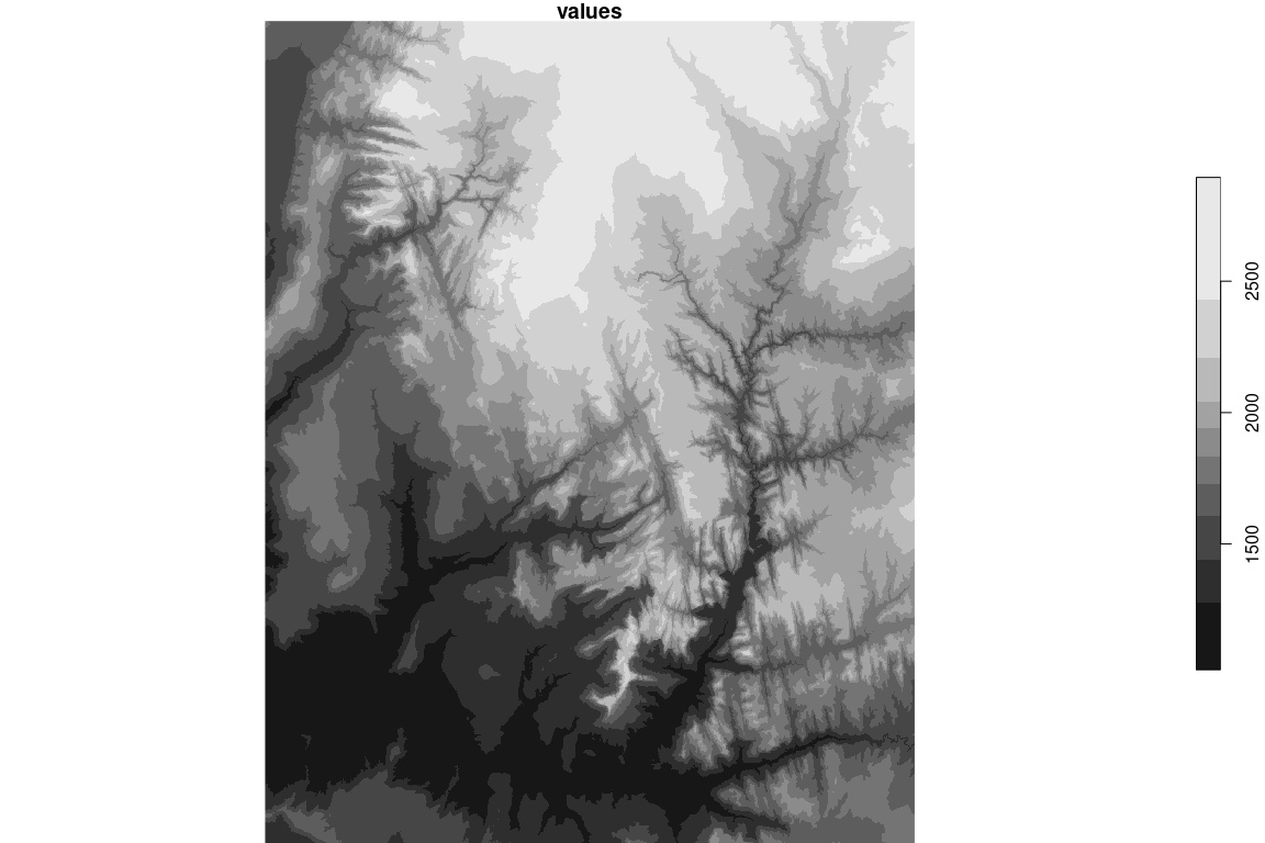 ``` r
## we can do this anywhere, in any projection but it depends on what our source *has* of course
## but, it's pretty general and powerful
gdalio_set_default_grid(list(extent = c(-1, 1, -1, 1) * 3e6,
dimension = c(768, 813),
projection = "+proj=stere +lat_0=-65 +lon_0=147"))
p <- gdalio_im(elevation.tiles.prod)
plot(p)
```
``` r
## we can do this anywhere, in any projection but it depends on what our source *has* of course
## but, it's pretty general and powerful
gdalio_set_default_grid(list(extent = c(-1, 1, -1, 1) * 3e6,
dimension = c(768, 813),
projection = "+proj=stere +lat_0=-65 +lon_0=147"))
p <- gdalio_im(elevation.tiles.prod)
plot(p)
```
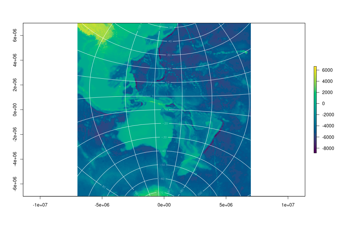
 My favourite projection family (I think) is Oblique Mercator. For a long
time I’ve wanted this kind of freedom and convenience for working with
spatial data … rather than constantly juggling objects and formats and
plumbing, more to come. :)
``` r
omerc <- "+proj=omerc +lonc=147 +gamma=9 +alpha=9 +lat_0=-10 +ellps=WGS84"
gdalio_set_default_grid(list(extent = c(-1, 1, -1, 1) * 7e6,
dimension = c(768, 813),
projection = omerc))
o <- gdalio_raster(elevation.tiles.prod)
raster::plot(o, col = hcl.colors(52))
xy <- reproj::reproj(raster::coordinates(o), "+proj=longlat", source = raster::projection(o))
xy[xy[,1] < 0, 1] <- xy[xy[,1] < 0, 1] + 360
library(raster)
#> Loading required package: sp
contour(raster::setValues(o, xy[,1]), add = TRUE, col = "white")
contour(setValues(o, xy[,2]), add = TRUE, col = "white")
```
My favourite projection family (I think) is Oblique Mercator. For a long
time I’ve wanted this kind of freedom and convenience for working with
spatial data … rather than constantly juggling objects and formats and
plumbing, more to come. :)
``` r
omerc <- "+proj=omerc +lonc=147 +gamma=9 +alpha=9 +lat_0=-10 +ellps=WGS84"
gdalio_set_default_grid(list(extent = c(-1, 1, -1, 1) * 7e6,
dimension = c(768, 813),
projection = omerc))
o <- gdalio_raster(elevation.tiles.prod)
raster::plot(o, col = hcl.colors(52))
xy <- reproj::reproj(raster::coordinates(o), "+proj=longlat", source = raster::projection(o))
xy[xy[,1] < 0, 1] <- xy[xy[,1] < 0, 1] + 360
library(raster)
#> Loading required package: sp
contour(raster::setValues(o, xy[,1]), add = TRUE, col = "white")
contour(setValues(o, xy[,2]), add = TRUE, col = "white")
```
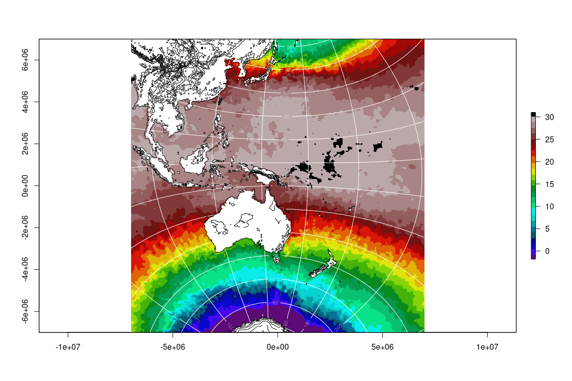
 The fun part is I can now change the source, I’ve already set up the map
I want and I can simply ask for a new set of pixels. The topography data
happens to be in Mercator from a tiled and level of detail image
service, while the SST is from a model output format (NetCDF) at a
single resolution. GDAL doesn’t care! Let’s make them the same:
``` r
sst <- gdalio_raster(f)
raster::plot(sst, col = palr::sst_pal(26))
contour(setValues(o, xy[,1]), add = TRUE, col = "white")
contour(setValues(o, xy[,2]), add = TRUE, col = "white")
contour(o, add = TRUE, labels = "", col = "black", levels = seq(0, 4500, by = 500))
```
The fun part is I can now change the source, I’ve already set up the map
I want and I can simply ask for a new set of pixels. The topography data
happens to be in Mercator from a tiled and level of detail image
service, while the SST is from a model output format (NetCDF) at a
single resolution. GDAL doesn’t care! Let’s make them the same:
``` r
sst <- gdalio_raster(f)
raster::plot(sst, col = palr::sst_pal(26))
contour(setValues(o, xy[,1]), add = TRUE, col = "white")
contour(setValues(o, xy[,2]), add = TRUE, col = "white")
contour(o, add = TRUE, labels = "", col = "black", levels = seq(0, 4500, by = 500))
```
 ## Code of Conduct
Please note that the gdalio project is released with a [Contributor Code
of
Conduct](https://contributor-covenant.org/version/2/0/CODE_OF_CONDUCT.html).
By contributing to this project, you agree to abide by its terms.
## Code of Conduct
Please note that the gdalio project is released with a [Contributor Code
of
Conduct](https://contributor-covenant.org/version/2/0/CODE_OF_CONDUCT.html).
By contributing to this project, you agree to abide by its terms.