---
title: "Introduction to Data Science"
subtitle: "Session 4: Functions and debugging"
author: "Simon Munzert"
institute: "Hertie School | [GRAD-C11/E1339](https://github.com/intro-to-data-science-23)" #"`r format(Sys.time(), '%d %B %Y')`"
output:
xaringan::moon_reader:
css: [default, 'simons-touch.css', metropolis, metropolis-fonts]
lib_dir: libs
nature:
highlightStyle: github
highlightLines: true
countIncrementalSlides: false
ratio: '16:9'
hash: true
---
```{css, echo=FALSE}
@media print { # print out incremental slides; see https://stackoverflow.com/questions/56373198/get-xaringan-incremental-animations-to-print-to-pdf/56374619#56374619
.has-continuation {
display: block !important;
}
}
```
```{r setup, include=FALSE}
# figures formatting setup
options(htmltools.dir.version = FALSE)
library(knitr)
opts_chunk$set(
comment = " ",
prompt = T,
fig.align="center", #fig.width=6, fig.height=4.5,
# out.width="748px", #out.length="520.75px",
dpi=300, #fig.path='Figs/',
cache=F, #echo=F, warning=F, message=F
engine.opts = list(bash = "-l")
)
## Next hook based on this SO answer: https://stackoverflow.com/a/39025054
knit_hooks$set(
prompt = function(before, options, envir) {
options(
prompt = if (options$engine %in% c('sh','bash')) '$ ' else 'R> ',
continue = if (options$engine %in% c('sh','bash')) '$ ' else '+ '
)
})
library(tidyverse)
library(nycflights13)
library(kableExtra)
```
# Table of contents
1. [Functions](#functions)
2. [Iteration](#iteration)
3. [Strategies for debugging](#debugging)
4. [Debugging R](#debuggingr)
---
class: inverse, center, middle
name: functions
# Functions
---
# Tidy programming basics
"Tidy programming" is not a strictly defined practice in the tidyverse. However, there are some common programming strategies that help you keep your code and workflow tidy. These include:
- Pipes (you already learned how to use them ✅)
- User-generated functions
- Functional programming with `purrr`
--
The latter two are extremely helpful - in particular when you are confronted with iterative tasks.
--
We will now learn the basics of creating your own functions and functional programming with R. There is much more to learn about these topics, so we will revisit them as the course progresses.
---
# Functional programming
R is a functional programming (FP) language. As Hadley Wickham puts it in [Advanced R](http://adv-r.had.co.nz/Functional-programming.html):
> This means that it provides many tools for the creation and manipulation of functions. In particular, R has what’s known as first-class functions. You can do anything with functions that you can do with vectors: you can assign them to variables, store them in lists, pass them as arguments to other functions, create them inside functions, and even return them as the result of a function.
R encourages you to use and build your own functions to solve problems. Often, this implies decomposing a large problem into small pieces, and solving each of them with independent functions.
There is much more to learn about functions and [functional programming](https://en.wikipedia.org/wiki/Functional_programming). Useful resources include:
- The chapter on functions in [R for Data Science](https://r4ds.had.co.nz/functions.html).
- The section on functional programming in [Advanced R](https://adv-r.hadley.nz/fp.html).
- The [R packages](https://r-pkgs.org/) book. In a way, bundling functions in a package is sometimes the next logical step.
---
# Creating functions
### Why creating functions?
That's a legit question. There are 18,000+ **packages** on CRAN (and many, many more on GitHub and other repositories) containing zillions of functions. Why should you create yet another one?
- Every data science project is unique. There are problems only you have to solve.
- For problems that are repetitive, you'll quickly look for options to automate the task.
- Functions are a great way to automate.
--
### Examples where creating functions makes sense
--
1. You want to scrape thousands of websites. This implies multiple steps, from downloading to parsing and cleaning. All these steps can be achieved with existing functions, but the fine-tuning is specific to the set of websites. You build one (or a set of) scraping functions that take the websites as input and return a cleaned data frame ready to be analyzed.
--
2. You want to estimate not one but multiple models on your dataset. The models vary both in terms of data input and specification. Again, based on existing modeling functions you tailor your own, allowing you to run all these models automatically and to parse the results into one clean data frame.
---
# Basic syntax
.pull-left[
Writing your own function in R is easy with the `function()` function1. The basic syntax is as follows:
```{r, eval = FALSE}
my_func <- function(ARGUMENTS) {
OPERATIONS
return(VALUE)
}
```
.footnote[1 Yes, a function to create functions. 🤯]
]
---
# Basic syntax
.pull-left[
Writing your own function in R is easy with the `function()` function1. The basic syntax is as follows:
```{r, eval = FALSE}
my_func <- function(ARGUMENTS) { #<<
OPERATIONS
return(VALUE)
}
```
- We write functions to apply them later. So, we have to give them a name. Here, we name it "`my_func`".
- Also, our function (almost) always needs input, plus we want to specify how exactly the function should behave. We can use arguments for this, which are specified as arguments of the `function()` function.
.footnote[1 Yes, a function to create functions. 🤯]
]
---
# Basic syntax
.pull-left[
Writing your own function in R is easy with the `function()` function1. The basic syntax is as follows:
```{r, eval = FALSE}
my_func <- function(ARGUMENTS) {
OPERATIONS #<<
return(VALUE)
}
```
- Next, we specify anything we want the function to do.
- This comes in between curly brackets, `{...}`.
- Importantly, we can recycle arguments by calling them by their name.
.footnote[1 Yes, a function to create functions. 🤯]
]
---
# Basic syntax
.pull-left[
Writing your own function in R is easy with the `function()` function1. The basic syntax is as follows:
```{r, eval = FALSE}
my_func <- function(ARGUMENTS) {
OPERATIONS
return(VALUE) #<<
}
```
- Finally, we specify what the function should return.
- This could be a list, data.frame, vector, sentence - or anything else really.
- Note that R automatically returns the final object that is written (not: assigned!) in your function by default. Still, my recommendation is that you get into the habit of assigning the return object(s) explicitly with `return()`.
.footnote[1 Yes, a function to create functions. 🤯]
]
---
# Basic syntax
.pull-left[
Writing your own function in R is easy with the `function()` function1. The basic syntax is as follows:
```{r, eval = FALSE}
my_func <- function(ARGUMENTS) {
OPERATIONS
return(VALUE)
} #<<
```
- Oh, and don't forget to close the curly brackets...
.footnote[1 Yes, a function to create functions. 🤯]
]
---
# Basic syntax
.pull-left[
Writing your own function in R is easy with the `function()` function1. The basic syntax is as follows:
```{r, eval = FALSE}
my_func <- function(ARGUMENTS) {
OPERATIONS
return(VALUE)
}
```
.footnote[1 Yes, a function to create functions. 🤯]
]
.pull-right[
Let's try it out with a simple example function - one that converts temperatures from [Fahrenheit to Celsius](https://en.wikipedia.org/wiki/Conversion_of_scales_of_temperature#Fahrenheit):2
```{r, eval = FALSE}
fahrenheit_to_celsius <- function(temp_F) {
temp_C <- (temp_F - 32) * (5/9)
return(temp_C)
}
```
.footnote[2 Courtesy of [Software Carpentry](https://swcarpentry.github.io/r-novice-inflammation/02-func-R/).]
]
---
# Basic syntax
.pull-left[
Writing your own function in R is easy with the `function()` function1. The basic syntax is as follows:
```{r, eval = FALSE}
my_func <- function(ARGUMENTS) {
OPERATIONS
return(VALUE)
}
```
.footnote[1 Yes, a function to create functions. 🤯]
]
.pull-right[
Let's try it out with a simple example function - one that converts temperatures from [Fahrenheit to Celsius](https://en.wikipedia.org/wiki/Conversion_of_scales_of_temperature#Fahrenheit):2
```{r, eval = FALSE}
fahrenheit_to_celsius <- function(temp_F) { #<<
temp_C <- (temp_F - 32) * (5/9)
return(temp_C)
}
```
- Our function has an intuitive name.
- Also, it takes just one thing as input, which we call `temp_F`.
.footnote[2 Courtesy of [Software Carpentry](https://swcarpentry.github.io/r-novice-inflammation/02-func-R/).]
]
---
# Basic syntax
.pull-left[
Writing your own function in R is easy with the `function()` function1. The basic syntax is as follows:
```{r, eval = FALSE}
my_func <- function(ARGUMENTS) {
OPERATIONS
return(VALUE)
}
```
.footnote[1 Yes, a function to create functions. 🤯]
]
.pull-right[
Let's try it out with a simple example function - one that converts temperatures from [Fahrenheit to Celsius](https://en.wikipedia.org/wiki/Conversion_of_scales_of_temperature#Fahrenheit):2
```{r, eval = FALSE}
fahrenheit_to_celsius <- function(temp_F) {
temp_C <- (temp_F - 32) * (5/9) #<<
return(temp_C)
}
```
- We now take up the argument `temp_F`, do something with it, and store the output in a new object, `temp_C`.
- Importantly, that object only lives within the function. When the function is run, we cannot access it from the environment.
.footnote[2 Courtesy of [Software Carpentry](https://swcarpentry.github.io/r-novice-inflammation/02-func-R/).]
]
---
# Basic syntax
.pull-left[
Writing your own function in R is easy with the `function()` function1. The basic syntax is as follows:
```{r, eval = FALSE}
my_func <- function(ARGUMENTS) {
OPERATIONS
return(VALUE)
}
```
.footnote[1 Yes, a function to create functions. 🤯]
]
.pull-right[
Let's try it out with a simple example function - one that converts temperatures from [Fahrenheit to Celsius](https://en.wikipedia.org/wiki/Conversion_of_scales_of_temperature#Fahrenheit):2
```{r, eval = FALSE}
fahrenheit_to_celsius <- function(temp_F) {
temp_C <- (temp_F - 32) * (5/9)
return(temp_C) #<<
}
```
- Finally, the output is returned.
.footnote[2 Courtesy of [Software Carpentry](https://swcarpentry.github.io/r-novice-inflammation/02-func-R/).]
]
---
# Basic syntax
.pull-left[
Writing your own function in R is easy with the `function()` function1. The basic syntax is as follows:
```{r, eval = FALSE}
my_func <- function(ARGUMENTS) {
OPERATIONS
return(VALUE)
}
```
.footnote[1 Yes, a function to create functions. 🤯]
]
.pull-right[
Let's try it out with a simple example function - one that converts temperatures from [Fahrenheit to Celsius](https://en.wikipedia.org/wiki/Conversion_of_scales_of_temperature#Fahrenheit):
```{r, eval = TRUE}
fahrenheit_to_celsius <- function(temp_F) {
temp_C <- (temp_F - 32) * (5/9)
return(temp_C)
}
```
Now, let's try out the function:
{{content}}
]
--
```{r, eval = TRUE}
fahrenheit_to_celsius(451)
```
{{content}}
--
Pretty hot, isn't it?
{{content}}
---
# Functions: default argument values, if(), else()
.pull-left[
Let's make the function a bit more complex, but also more fun.
]
.pull-right[
```{r, eval = FALSE}
temp_convert <-
function(temp, from = "f") {
if (!(from %in% c("f", "c"))){
stop("No valid input
temperature specified.")
}
if (from == "f") {
out <- (temp - 32) * (5/9)
} else {
out <- temp * (9/5) + 32
}
if((from == "c" & temp > 30) |
(from == "f" & out > 30)) {
message("That's damn hot!")
}else{
message("That's not so hot.")
}
return(out) # return temperature
}
```
]
---
# Functions: default argument values, if(), else()
.pull-left[
Let's make the function a bit more complex, but also more fun.
- By giving `from` a default value (`"f"`), we ensure that the function returns valid output when only the key input, `temp`, is provided.
]
.pull-right[
```{r, eval = FALSE}
temp_convert <-
function(temp, from = "f") { #<<
if (!(from %in% c("f", "c"))){
stop("No valid input
temperature specified.")
}
if (from == "f") {
out <- (temp - 32) * (5/9)
} else {
out <- temp * (9/5) + 32
}
if((from == "c" & temp > 30) |
(from == "f" & out > 30)) {
message("That's damn hot!")
}else{
message("That's not so hot.")
}
return(out) # return temperature
}
```
]
---
# Functions: default argument values, if(), else()
.pull-left[
Let's make the function a bit more complex, but also more fun.
- By giving `from` a default value (`"f"`), we ensure that the function returns valid output when only the key input, `temp`, is provided.
- `if() {...}` allows us to make conditional statements. Here, we test for the validity of the input for argument `from`.
]
.pull-right[
```{r, eval = FALSE}
temp_convert <-
function(temp, from = "f") {
if (!(from %in% c("f", "c"))){ #<<
stop("No valid input
temperature specified.")
}
if (from == "f") {
out <- (temp - 32) * (5/9)
} else {
out <- temp * (9/5) + 32
}
if((from == "c" & temp > 30) |
(from == "f" & out > 30)) {
message("That's damn hot!")
}else{
message("That's not so hot.")
}
return(out) # return temperature
}
```
]
---
# Functions: default argument values, if(), else()
.pull-left[
Let's make the function a bit more complex, but also more fun.
- By giving `from` a default value (`"f"`), we ensure that the function returns valid output when only the key input, `temp`, is provided.
- `if() {...}` allows us to make conditional statements. Here, we test for the validity of the input for argument `from`.
- If the condition is not met, the function breaks and prints a message.
]
.pull-right[
```{r, eval = FALSE}
temp_convert <-
function(temp, from = "f") {
if (!(from %in% c("f", "c"))){
stop("No valid input
temperature specified.") #<<
}
if (from == "f") {
out <- (temp - 32) * (5/9)
} else {
out <- temp * (9/5) + 32
}
if((from == "c" & temp > 30) |
(from == "f" & out > 30)) {
message("That's damn hot!")
}else{
message("That's not so hot.")
}
return(out) # return temperature
}
```
]
---
# Functions: default argument values, if(), else()
.pull-left[
Let's make the function a bit more complex, but also more fun.
- By giving `from` a default value (`"f"`), we ensure that the function returns valid output when only the key input, `temp`, is provided.
- `if() {...}` allows us to make conditional statements. Here, we test for the validity of the input for argument `from`.
- If the condition is not met, the function breaks and prints a message.
- With `else()`, we specify what to do if the `if()` condition is not met.
]
.pull-right[
```{r, eval = FALSE}
temp_convert <-
function(temp, from = "f") {
if (!(from %in% c("f", "c"))){
stop("No valid input
temperature specified.")
}
if (from == "f") {
out <- (temp - 32) * (5/9)
} else { #<<
out <- temp * (9/5) + 32
}
if((from == "c" & temp > 30) |
(from == "f" & out > 30)) {
message("That's damn hot!")
}else{
message("That's not so hot.")
}
return(out) # return temperature
}
```
]
---
# Functions: default argument values, if(), else()
.pull-left[
Let's make the function a bit more complex, but also more fun.
- By giving `from` a default value (`"f"`), we ensure that the function returns valid output when only the key input, `temp`, is provided.
- `if() {...}` allows us to make conditional statements. Here, we test for the validity of the input for argument `from`.
- If the condition is not met, the function breaks and prints a message.
- We `else()` we specify what to do if the `if()` condition is not met.
- Make R more talkative with `message()`. Future-You will like it!
]
.pull-right[
```{r, eval = FALSE}
temp_convert <-
function(temp, from = "f") {
if (!(from %in% c("f", "c"))){
stop("No valid input
temperature specified.")
}
if (from == "f") {
out <- (temp - 32) * (5/9)
} else {
out <- temp * (9/5) + 32
}
if((from == "c" & temp > 30) |
(from == "f" & out > 30)) {
message("That's damn hot!") #<<
}else{
message("That's not so hot.") #<<
}
return(out) # return temperature
}
```
]
---
# Anonymous functions
In R, functions are objects in their own right. They aren’t automatically bound to a name. If you choose not to give the function a name, you get an **anonymous function**. You use an anonymous function when it’s not worth the effort to give it a name.
--
**Examples:**
```{r, eval = FALSE}
map(char_vec, function(x) paste(x, collapse = "|"))
integrate(function(x) sin(x) ^ 2, 0, pi)
```
---
# Anonymous functions
In R, functions are objects in their own right. They aren’t automatically bound to a name. If you choose not to give the function a name, you get an **anonymous function**. You use an anonymous function when it’s not worth the effort to give it a name.
As of `R 4.1.0`, there's a new shorthand syntax for anonymous functions: `\(x)`.
--
**Example:**
```{r, eval = TRUE}
(function (x) {paste(x, 'is awesome!')})('Data science') # old syntax
(\(x) {paste(x, 'is awesome!')})('Data science') # new syntax
```
---
# Anonymous functions
In R, functions are objects in their own right. They aren’t automatically bound to a name. If you choose not to give the function a name, you get an **anonymous function**. You use an anonymous function when it’s not worth the effort to give it a name.
As of `R 4.1.0`, there's a new shorthand syntax for anonymous functions: `\(x)`. This plays along nicely with the (native) pipe when we want to pass content to the RHS but not to the first argument.
**Example:**
```{r, eval = FALSE}
mtcars |> subset(cyl == 4) |> (\(x) lm(mpg ~ disp, data = x))()
```
---
# `...` (Dot-dot-dot)
Functions can have a special argument `...` (pronounced *dot-dot-dot*). In other programming languages, this type of argument is often called varargs (short for variable arguments), or ellipsis. With it, a function can take any number of additional arguments. That is potentially very powerful!
A common application is to use `...` to pass those additional arguments on to another function.
--
.pull-left[
**Toy example:**
```{r, eval = TRUE}
my_list_generator <- function(y, z) {
list(y = y, z = z)
}
my_list_generator_2 <- function(x, ...) {
my_list_generator(...)
}
str(my_list_generator_2(x = 1, y = 2, z = 3))
```
]
--
.pull-right[
**Real-life example:**
```{r, eval = FALSE}
map(.x, .f, ...)
map(mtcars, mean, na.rm = TRUE)
```
Arguments:
- `.x`: A list or atomic vector
- `.f`: A function
- `...`: Additional arguments passed on to the mapped function.
]
---
# Writing functions with ChatGPT
.pull-left-wide[
Not every function you plan to write is unique, nor is every problem you want to solve functionally.
ChatGPT and other AI-based coding tools can help you a lot in finding functional solutions you can describe but not verbalize (yet).
I encourage you to use AI for this purpose, but be aware of the necessity to (a) debug and (b) assign credit where due.
**Let's try it out with one of the following prompts:**
- *Write an R function that capitalizes the first letter of each word in a character vector.*
- *Write an R function that allows me to play one round of black jack.*
]
.pull-right-small[
]
---
class: inverse, center, middle
name: iteration
# Iteration
---
# Iteration
### The ubiquity of iteration
- Often we have to run the same task over and over again, with minor variations. Examples:
- Standardize values of a variable
- Recode all numeric variables in a dataset
- Running multiple models with varying covariate sets
- A benefit of scripting languages in data (as opposed to point-and-click solutions) is that we can easily automate the process of iteration
--
### Ways to iterate
- A simple approach is to copy-and-paste code with minor modifications (→ "[duplicate code](https://en.wikipedia.org/wiki/Duplicate_code)", → "[copy-and-paste programming](https://en.wikipedia.org/wiki/Copy-and-paste_programming)"). This is lazy, error-prone, not very efficient, and violates the "[Don't repeat yourself](https://en.wikipedia.org/wiki/Don%27t_repeat_yourself)" (DRY) principle.
- In R, [vectorization](https://adv-r.hadley.nz/perf-improve.html#vectorise), that is applying a function to every element of a vector at once, already does a good share of iteration for us.
- `for()` [loops](https://r4ds.had.co.nz/iteration.html) are intuitive and straightforward to build, but sometimes not very efficient.
- Finally, we learned about functions. Now, we learn how to unleash their power by applying them to anything we interact with in R at scale.
---
# Iteration with purrr
.pull-left-wide[
### The tidyverse way to iterate
- For *real* functional programming in base R, we can use the `*apply()` family of functions (`lapply()`, `sapply()`, etc.). See [here](https://nsaunders.wordpress.com/2010/08/20/a-brief-introduction-to-apply-in-r/) for an excellent summary.
- In the tidyverse, this functionality comes with the `purrr` package.
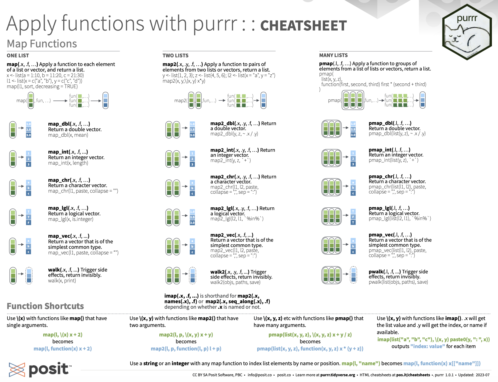
- At its core is the `map*()` family of functions.
### How `purrr` works
- The idea is always to **apply** a function to **x**, where x can be a list, vector, data.frame, or something more complex.
- The output is then returned as output of a pre-defined type (e.g., a list).
]
.pull-right-small-center[
]
---
# Iteration with purrr: map()
The `map*()` functions all follow a similar syntax:
`map(.x, .f, ...)`
We use it to apply a function `.f` to each piece in `.x`. Additional arguments to `.f` can be passed on in `...`.
--
For instance, if we want to identify the object class of every column of a data.frame, we can write:
```{r}
map(starwars, class)
```
---
# Iteration with purrr: map() *cont.*
By default, `map()` returns a list. But we can also use other `map*()` functions to give us an atomic vector of an indicated type (e.g., `map_int()` to return an integer vector, or `map_vec()` to return a vector that is the simplest common type).
Going back to the previous example, we can also use `map_chr()`, which returns a character vector:
```{r}
map_chr(starwars, class)
```
--
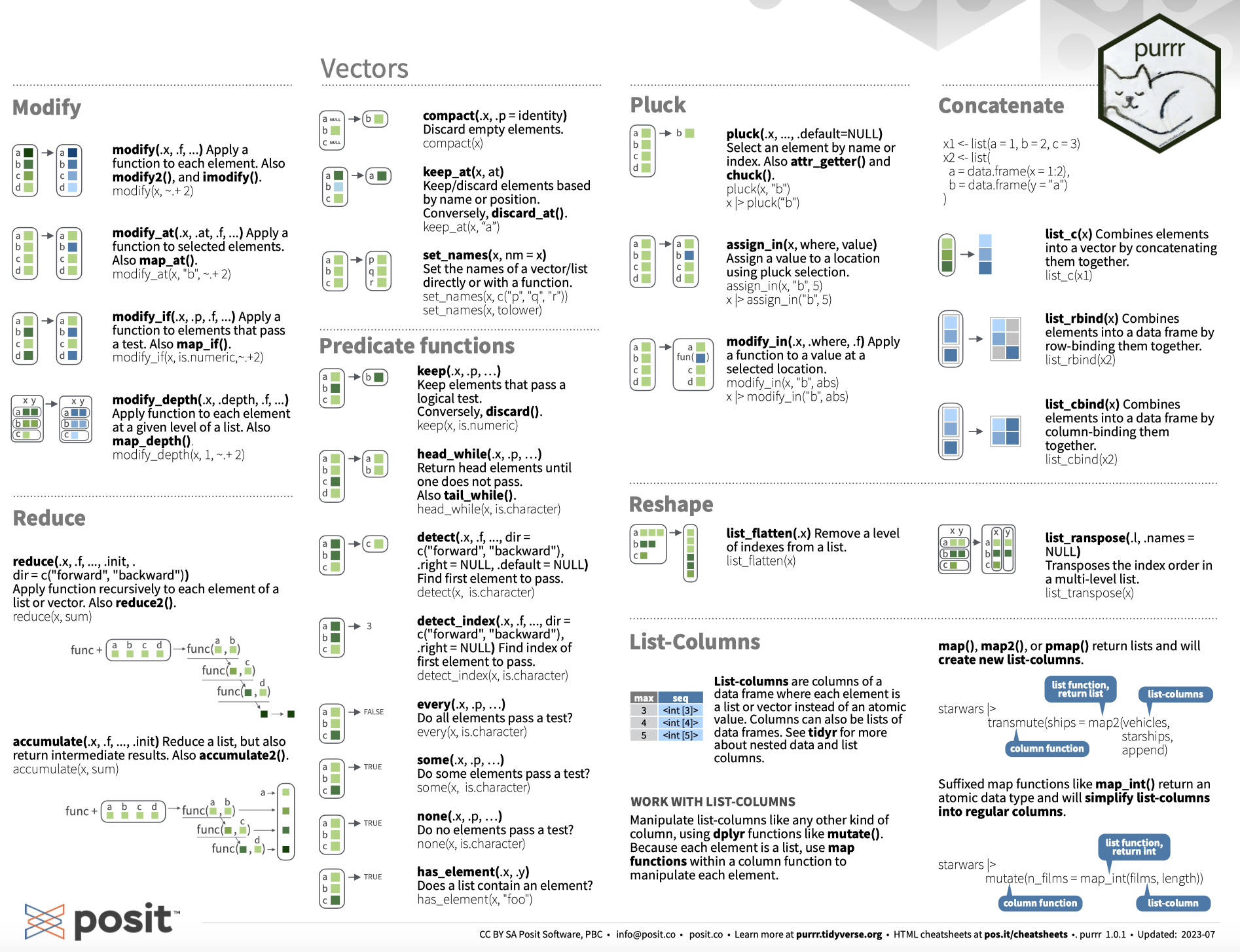
The `purrr` function set is quite comprehensive. Be sure to check out the [cheat sheet](https://github.com/rstudio/cheatsheets/blob/master/purrr.pdf) and the [tutorials](https://jennybc.github.io/purrr-tutorial/index.html). You'll survive without `purrr` but you probably don't want to live without it. Together with `dplyr` it's easily the most powerful package for data wrangling in the tidyverse. If you master it, it will save you a lot of time and headaches.
---
# Iteration with purrr: map() *cont.*
---
# Iteration with purrr: map() *cont.*
---
class: inverse, center, middle
name: debugging
# Strategies for debugging
---
# What's debugging?
.pull-left[
### Straight from the [Wikipedia](https://en.wikipedia.org/wiki/Debugging)
"Debugging is the process of finding and resolving bugs (defects or problems that prevent correct operation) within computer programs, software, or systems."
### A famous (yet not the first) bug:
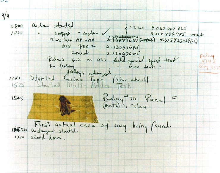
The term "bug" was used in an account by computer pioneer [Grace Hopper](https://en.wikipedia.org/wiki/Grace_Hopper) (see on the right). While she was working on a [Mark II](https://en.wikipedia.org/wiki/Harvard_Mark_II) computer at Harvard University, her associates discovered a moth stuck in a relay and thereby impeding operation, whereupon she remarked that they were "debugging" the system. This bug was carefully removed and taped to the log book (see on the right).
]
.pull-right-center[
 Above:
 Grace Hopper,
Below: The bug

]
---
# Why debugging matters
.pull-left-wide[
The Wikipedia [list of software bugs](https://en.wikipedia.org/wiki/List_of_software_bugs) with significant consequences is growing and you don't want to be on it.
NASA software engineers are [famous for producing bug-free code](https://www.bugsplat.com/blog/less-serious/why-nasa-code-doesnt-crash/). This was learned the hard and costly way though. Some highlights from space:
- 1962: A booster went off course during launch, resulting in the [destruction of NASA Mariner 1](https://www.youtube.com/watch?v=CkOOazEJcUc) . This was the result of the failure of a transcriber to notice an overbar in a handwritten specification for the guidance program, resulting in an incorrect formula the FORTRAN code.
- 1999: [NASA's Mars Climate Orbiter was destroyed](https://www.youtube.com/watch?v=lcYkOh4nweE), due to software on the ground generating commands based on parameters in pound-force (lbf) rather than newtons (N)
- 2004: [NASA's Spirit rover became unresponsive](https://www.youtube.com/watch?v=7V54LRRJaGk) on January 21, 2004, a few weeks after landing on Mars. Engineers found that too many files had accumulated in the rover's flash memory (the problem could be fixed though by deleting unnecessary files, and the Rover lived happily ever after. Until it [froze to death in 2011](https://en.wikipedia.org/wiki/Spirit_(rover)).
]
.pull-right-small[
]
---
# Why debugging matters (cont.)
---
# Why debugging matters (cont.)
.pull-left-center[
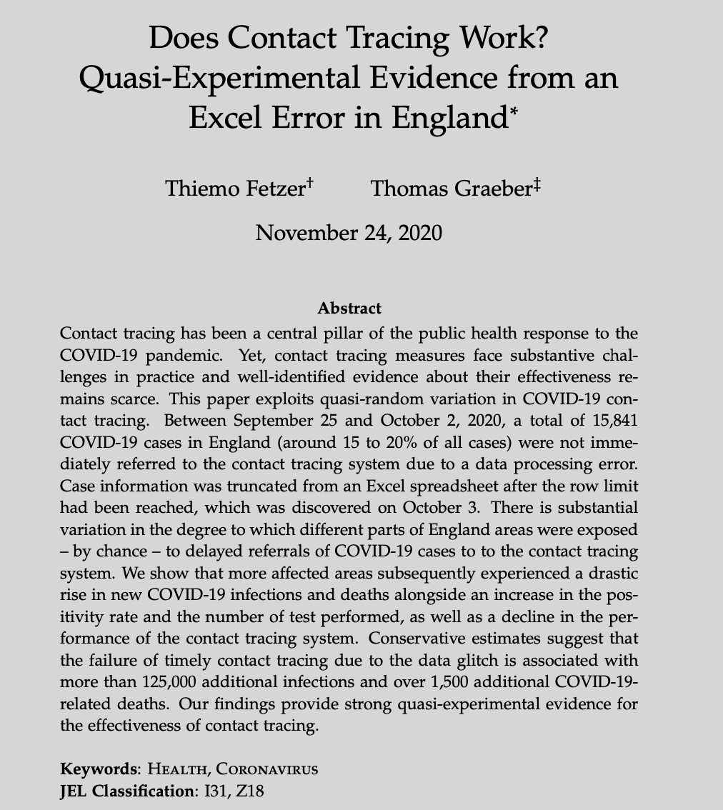
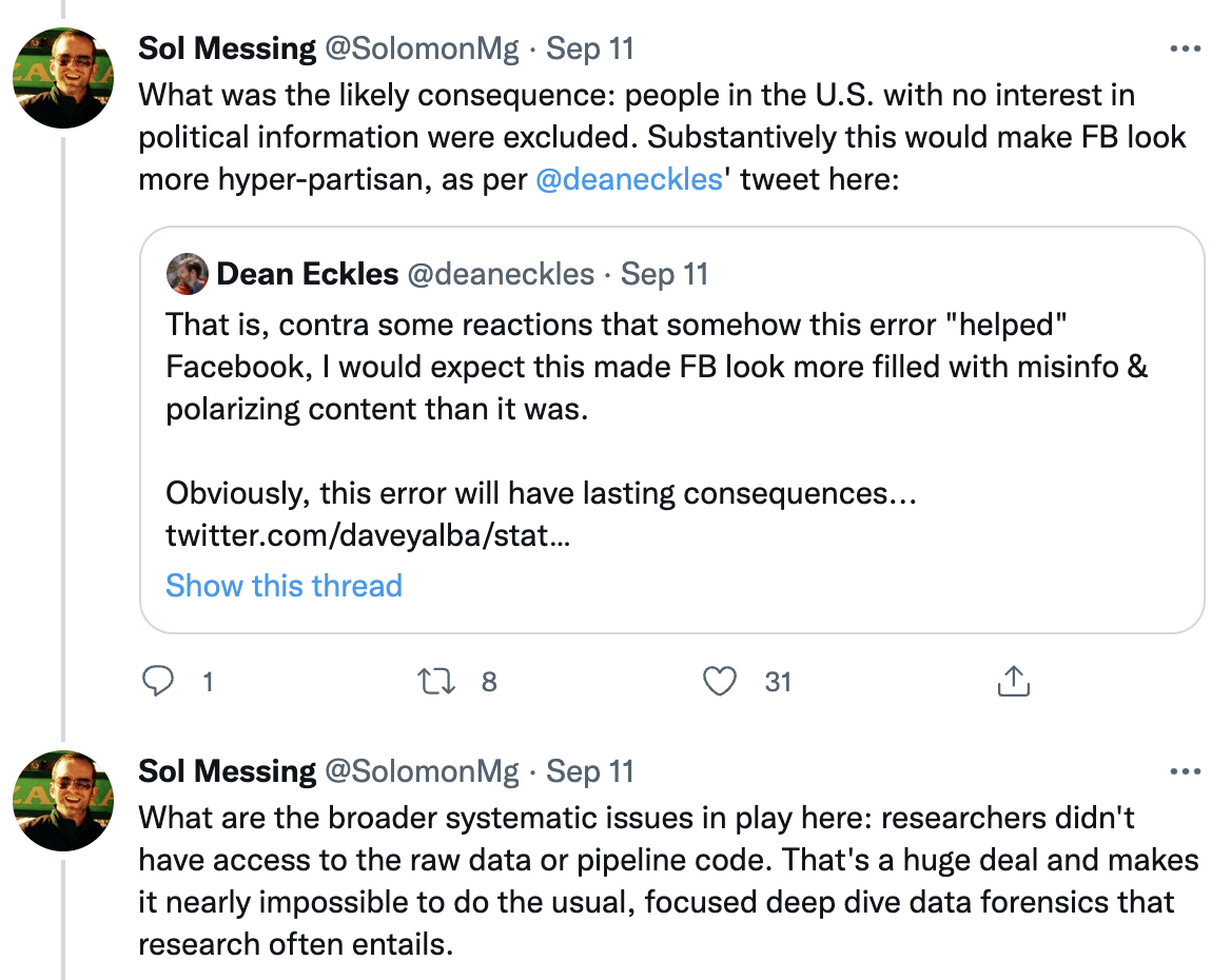
`Source` [Washington Post](https://www.washingtonpost.com/technology/2021/09/10/facebook-error-data-social-scientists/)
]
.pull-right-center[
`Source` [Solomon Messing / Twitter](https://twitter.com/solomonmg/status/1436742352039669760)
]
---
# A general strategy for debugging
.pull-left-vsmall[]
.pull-right-wide[
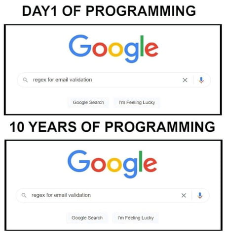
## 1. Google
## 2. Reset
## 3. Debug
## 4. Deter
]
---
# Google
.footnote[1Do you get an error message you don't understand? That's good news actually, because the really nasty bugs come without errors. ]
.pull-left-wide2[
According to [this analysis](https://github.com/noamross/zero-dependency-problems/blob/master/misc/stack-overflow-common-r-errors.md), the most common error types in R are:1
1. `Could not find function` errors, usually caused by typos or not loading a required package.
2. `Error in if` errors, caused by non-logical data or missing values passed to R's `if` conditional statement.
3. `Error in eval` errors, caused by references to objects that don't exist.
4. `Cannot open` errors, caused by attempts to read a file that doesn't exist or can't be accessed.
5. `no applicable method` errors, caused by using an object-oriented function on a data type it doesn't support.
6. `subscript out of bounds` errors, caused by trying to access an element or dimension that doesn't exist
7. Package errors caused by being unable to install, compile or load a package.
]
--
.pull-right-small2[
Whenever you see an error message, start by [googling](https://lmgtfy.app/?q=Error+in+interpretative_method+%3A+%20+%20could+not+find+function+%22interpretative_method%22&iie=1) it. Improve your chances of a good match by removing any variable names or values that are specific to your problem. Also, look for [Stack Overflow](https://stackoverflow.com/questions/tagged/r) posts and list of answers.
]
---
# Reset
.pull-left[
- If at first you don't succeed, try exactly the same thing again.
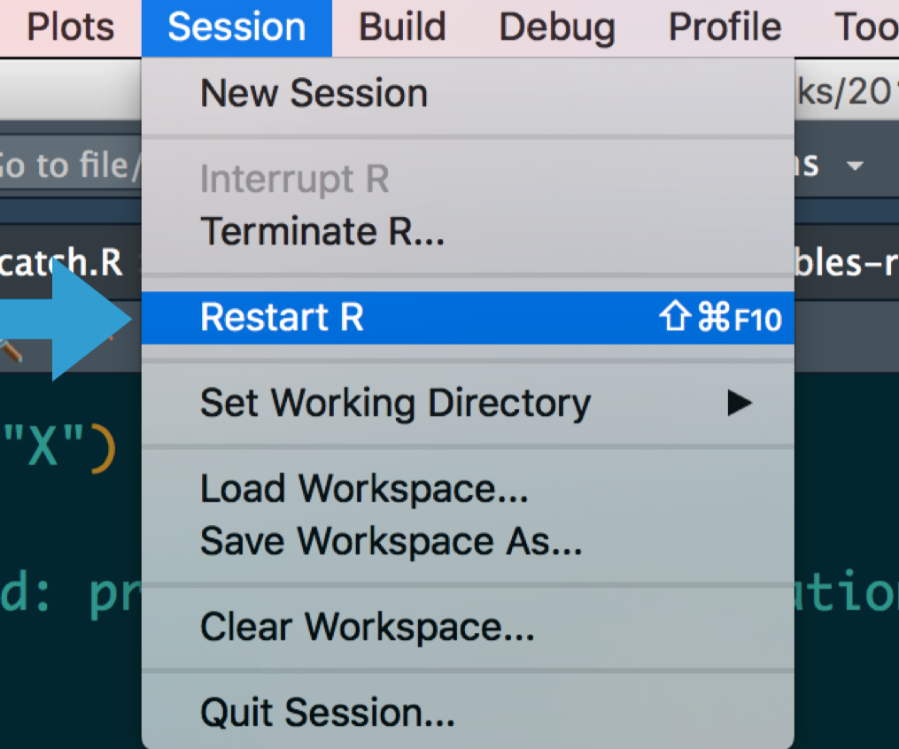
- Have you tried turning it off and on again?
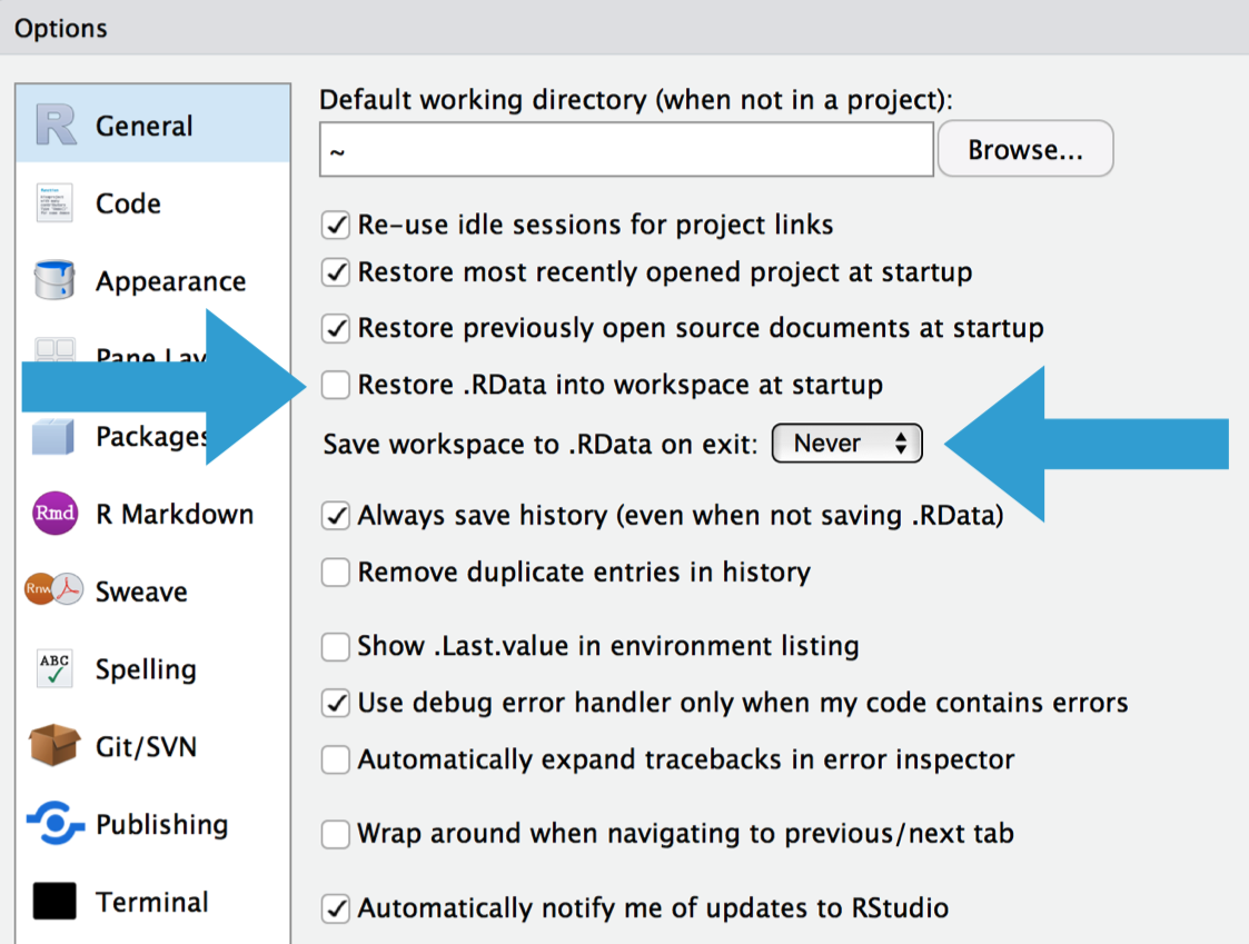
- Do you use `rm(list = ls())`? Don't. Packages remain loaded, options and environment variables set, ... all possible sources of error!
- A fresh start clears the workspace, resets options, environment variables, and the path.
- While we're at it, check out James Wade's advice ["How I set up RStudio for Efficient Coding" (YouTube)](https://www.youtube.com/watch?v=p-r-AWR3-Es).
]
.pull-right[
]
---
# Debug
### Make the error repeatable.
- Execute the code many times as you consider and reject hypotheses. To make that iteration as quick possible, it’s worth some upfront investment to make the problem both easy and fast to reproduce.
- Work with reproducible and minimal examples by removing innocuous code and simplifying data.
- Consider automated testing. Add some nearby tests to ensure that existing good behaviour is preserved.
### Track the error down.
- Execute code step by step and inspect intermediate outputs.
- Adopt the scientific method: Generate hypotheses, design experiments to test them, and record your results.
### Once found, fix the error and test it.
- Ensure you haven’t introduced any new bugs in the process.
- Make sure to carefully record the correct output, and check against the inputs that previously failed.
- Reset and run again to make sure everything still works.
---
# Deter
.pull-left-wide2[
### Defensive programming
- **Pay attention.** Do results make sense? Do they look different from previous results? Why?
- **Know what you're doing**, and what you're expecting.
- Avoid functions that return different types of output depending on their input, e.g., `[]` and `sapply()`.
- Be strict about what you accept (e.g., only scalars).
- Avoid functions that use non-standard evaluation (e.g., `with()`)
- **Fail fast**.
- As soon as something wrong is discovered, signal an error.
- Add tests (e.g., with the `testthat` package).
- Practice good condition/exception handling, e.g., with `try()` and `tryCatch()`.
- Write error messages for humans.
]
.pull-right-small3[
### Transparency
- Collaborate! [Pair programming](https://en.wikipedia.org/wiki/Pair_programming) is an established software development technique that increases code robustness. It also works [from remote](https://ivelasq.rbind.io/blog/vscode-live-share/).
- Be transparent! Let others access your code and comment on it.
]
---
class: inverse, center, middle
name: debuggingr
# Debugging R
---
# What you get
Error : .onLoad failed in loadNamespace() for 'rJava', details:
call: dyn.load(file, DLLpath = DLLpath, ...)
error: unable to load shared object '/Users/janedoe/Library/R/3.6/library/rJava/libs/rJava.so':
libjvm.so: cannot open shared object file: No such file or directory
Error: loading failed
Execution halted
ERROR: loading failed
* removing '/Users/janedoe/Library/R/3.6/library/rJava/'
Warning in install.packages :
installation of package 'rJava' had non-zero exit status
`Credit` [Jenny Bryan](https://github.com/jennybc/debugging)
---
# What you see
Error : blah failed blah blah() blah 'blah', blah:
call: blah.blah(blah, blah = blah, ...)
error: unable to blah blah blah '/blah/blah/blah/blah/blah/blah/blah/blah/blah.so':
blah.so: cannot open blah blah blah: No blah blah blah blah
Error: blah failed
blah blah
ERROR: blah failed
* removing '/blah/blah/blah/blah/blah/blah/blah/'
Warning in blah.blah :
blah of blah 'blah' blah blah-blah blah blah
`Credit` [Jenny Bryan](https://github.com/jennybc/debugging)
---
# Strategies to debug your R code
Sometimes the mistake in your code is hard to diagnose, and googling doesn't help. Here are a couple of strategies to debug your code:
- Use `traceback()` to determine where a given error is occurring.
- Output diagnostic information in code with `print()`, `cat()` or `message()` statements.
- Use `browser()` to open an interactive debugger before the error
- Use `debug()` to automatically open a debugger at the start of a function call.
- Use `trace()` to make temporary code modifications inside a function that you don't have easy access to.
---
# Locating errors with traceback()
.pull-left[
### Motivation and usage
- When an error occurs with an unidentifiable error message or an error message that you are in principle familiar with but cannot locate its sources, the `traceback()` function comes in handy.
- The `traceback()` function prints the sequence of calls that led to an uncaught error.
- The `traceback()` output reads from bottom to top.
- Note that errors caught via `try()` or `tryCatch()` do not generate a traceback!
- If you’re calling code that you `source()`d into R, the traceback will also display the location of the function, in the form `filename.r#linenumber`.
]
--
.pull-right[
### Example
In the call sequence below, the execution of `g()` triggers an error:
```{r, eval = FALSE}
f <- function(x) x + 1
g <- function(x) f(x)
g("a")
```
```r
#> Error in x + 1 : non-numeric argument to binary operator
```
Doing the traceback reveals that the function call f(x) is what lead to the error:
```{r, eval = FALSE}
traceback()
```
```r
#> 2: f(x) at #1
#> 1: g("a")
```
]
---
# Interactive debugging with browser()
.pull-left[
### Motivation and usage
- Sometimes, you need more information than the precise location of an error in a function to fix it.
- The interactive debugger lets you pause the run of a function and interactively explore its state.
- Two options to enter the interactive debugger:
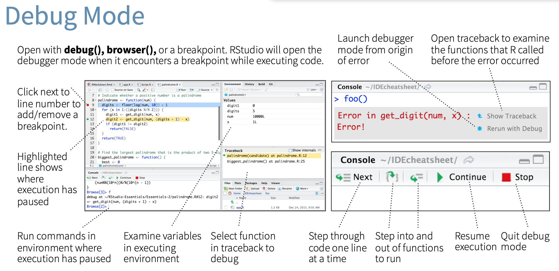
1. Through RStudio's "Rerun with Debug" tool, shown to the right of an error message.
2. You can insert a call to `browser()` into the function at the stage where you want to pause, and re-run the function.
- In either case, you’ll end up in an interactive environment inside the function where you can run arbitrary R code to explore the current state. You’ll know when you’re in the interactive debugger because you get a special prompt, `Browse[1]>`.
]
--
.pull-right[
### Example
```{r, eval = FALSE}
h <- function(x) x + 3
g <- function(b) {
browser() #<<
h(b)
}
g(10)
```
Some useful things to do are:
1. Use `ls()` to determine what objects are available in the current
environment.
2. Use `str()`, `print()` etc. to examine the objects.
3. Use `n` to evaluate the next statement.
4. Use `s`: like `n` but also step into function calls.
5. Use `where` to print a stack trace (→ traceback).
6. Use `c` to exit debugger and continue execution.
7. Use `Q` to exit debugger and return to the R prompt.
]
---
# Debugging other peoples' code
.pull-left[
### Motivation
- Sometimes the error is outside your code in a package you're using, you might still want to be able to debug.
- Two options:
1. Get a local version of the package code and debug as if it were your own.
2. Use functions which which allow you to start a browser in existing functions, including `recover()` and `debug()`.
]
.pull-right[
]
---
# Debugging other peoples' code (cont.)
.pull-left-small[
### Motivation
- `recover()` serves as an alternative error handler which you activate by calling `options(error = recover)`.
- You can then select from a list of current calls to browse.
- `options(error = NULL)` turns off this debugging mode again.
- A simpler alternative is `options(error = browser)`, but this only allows you to browse the call where the error occurred.
]
--
.pull-right-wide[
### Example
- Activate debugging mode; then execute (flawed) function:
```{r, eval = FALSE}
options(error = recover) #<<
lm(mpg ~ wt, data = "mtcars")
```
```r
Error in model.frame.default(formula = mpg ~ wt, data = "mtcars", drop.unused.levels = TRUE)
'data' must be a data.frame, environment, or list
Enter a frame number, or 0 to exit
1: lm(mpg ~ wt, data = "mtcars")
2: eval(mf, parent.frame())
3: eval(mf, parent.frame())
Selection:
```
- Deactivate debugging mode:
```{r, eval = FALSE}
options(error = NULL) #<<
```
]
---
# Debugging other peoples' code (cont.)
.pull-left[
### Motivation
- `debug()` activates the debugger on any function, including those in packages (see on the right). `undebug()` deactivates the debugger again.
- Some functions in another package are easier to find than others. There are
- *exported* functions which are available outside of a package and
- *internal* functions which are only available within a package.
- To find (and debug) exported functions, use the `::` syntax, as in `ggplot2::ggplot`.
- To find un-exported functions, use the `:::` syntax, as in `ggplot2:::check_required_aesthetics`.
]
--
.pull-right[
### Example
- Activate debugging mode for `lm()` function; then execute function:
```{r, eval = FALSE}
debug(stats::lm) #<<
lm(mpg ~ weight, data = "mtcars")
```
- Interactive debugging mode for `lm()` is entered; use the common `browser()` functionality to navigate:
```r
debugging in: lm(mpg ~ weight, data = mtcars)
debug: {
ret.x <- x
...
Browse[2]>
```
- Deactivate debugging mode:
```{r, eval = FALSE}
undebug(stats::lm) #<<
```
]
---
# Debugging in RStudio
---
# More on debugging R
.pull-left[
### Further reading
- [12-minute video](https://vimeo.com/99375765) on debugging in R
- Jenny Bryan's [talk on debugging](https://github.com/jennybc/debugging) at rstudio::conf 2020
- Jenny Bryan and Jim Hester's "What They Forgot to Teach You About R", Chapter 11: [Debugging R code](https://rstats.wtf/debugging-r)
- Jonathan McPherson's [Debugging with RStudio](https://support.rstudio.com/hc/en-us/articles/205612627-Debugging-with-RStudio)
]
.pull-right[
]
---
# Next steps
### Assignment
Assignment 2 is online! You have a bit more than a week to work on it - final upload deadline is Oct 4.
### Next lecture
**Relational databases and SQL.** Buckle up and bring coffee, because it'll get both exciting and tedious at the same time.


