{
"cells": [
{
"cell_type": "markdown",
"metadata": {},
"source": [
"# Visualize JAX model metrics with TensorBoard\n",
"\n",
"[](https://colab.research.google.com/github/jax-ml/jax-ai-stack/blob/main/docs/source/JAX_visualizing_models_metrics.ipynb)"
]
},
{
"cell_type": "markdown",
"metadata": {},
"source": [
"To keep things straightforward and familiar, we reuse the model and data from [Getting started with JAX for AI](https://jax-ai-stack.readthedocs.io/en/latest/neural_net_basics.html) - if you haven't read that yet and want the primer, start there before returning.\n",
"\n",
"All of the modeling and training code is the same here. What we have added are the tensorboard connections and the discussion around them."
]
},
{
"cell_type": "code",
"execution_count": 12,
"metadata": {},
"outputs": [],
"source": [
"import tensorflow as tf\n",
"import io\n",
"from datetime import datetime"
]
},
{
"cell_type": "code",
"execution_count": 2,
"metadata": {
"id": "hKhPLnNxfOHU",
"outputId": "ac3508f0-ccc6-409b-c719-99a4b8f94bd6"
},
"outputs": [],
"source": [
"from sklearn.datasets import load_digits\n",
"digits = load_digits()"
]
},
{
"cell_type": "markdown",
"metadata": {},
"source": [
"Here we set the location of the tensorflow writer - the organization is somewhat arbitrary, though keeping a folder for each training run can make later navigation more straightforward."
]
},
{
"cell_type": "code",
"execution_count": 13,
"metadata": {},
"outputs": [],
"source": [
"file_path = \"runs/test/\" + datetime.now().strftime(\"%Y%m%d-%H%M%S\")\n",
"test_summary_writer = tf.summary.create_file_writer(file_path)"
]
},
{
"cell_type": "markdown",
"metadata": {},
"source": [
"Pulled from the official tensorboard examples, this convert function makes it simple to drop matplotlib figures directly into tensorboard"
]
},
{
"cell_type": "code",
"execution_count": 4,
"metadata": {},
"outputs": [],
"source": [
"def plot_to_image(figure):\n",
" \"\"\"Sourced from https://www.tensorflow.org/tensorboard/image_summaries\n",
" Converts the matplotlib plot specified by 'figure' to a PNG image and\n",
" returns it. The supplied figure is closed and inaccessible after this call.\"\"\"\n",
" # Save the plot to a PNG in memory.\n",
" buf = io.BytesIO()\n",
" plt.savefig(buf, format='png')\n",
" # Closing the figure prevents it from being displayed directly inside\n",
" # the notebook.\n",
" plt.close(figure)\n",
" buf.seek(0)\n",
" # Convert PNG buffer to TF image\n",
" image = tf.image.decode_png(buf.getvalue(), channels=4)\n",
" # Add the batch dimension\n",
" image = tf.expand_dims(image, 0)\n",
" return image"
]
},
{
"cell_type": "markdown",
"metadata": {},
"source": [
"Whereas previously the example displays the training data snapshot in the notebook, here we stash it in the tensorboard images. If a given training is to be repeated many, many times it can save space to stash the training data information as its own run and skip this step for each subsequent training, provided the input is static. Note that this pattern uses the writer in a `with` context manager. We are able to step into and out of this type of context through the run without losing the same file/folder experiment."
]
},
{
"cell_type": "code",
"execution_count": 5,
"metadata": {
"id": "Y8cMntSdfyyT",
"outputId": "9343a558-cd8c-473c-c109-aa8015c7ae7e"
},
"outputs": [],
"source": [
"import matplotlib.pyplot as plt\n",
"\n",
"fig, axes = plt.subplots(10, 10, figsize=(6, 6),\n",
" subplot_kw={'xticks':[], 'yticks':[]},\n",
" gridspec_kw=dict(hspace=0.1, wspace=0.1))\n",
"\n",
"for i, ax in enumerate(axes.flat):\n",
" ax.imshow(digits.images[i], cmap='binary', interpolation='gaussian')\n",
" ax.text(0.05, 0.05, str(digits.target[i]), transform=ax.transAxes, color='green')\n",
"with test_summary_writer.as_default():\n",
" tf.summary.image(\"Training Data\", plot_to_image(fig), step=0)"
]
},
{
"cell_type": "markdown",
"metadata": {},
"source": [
"After running all above and launching `tensorboard --logdir runs/test` from the same folder, you should see the following in the supplied URL:\n",
"\n",
"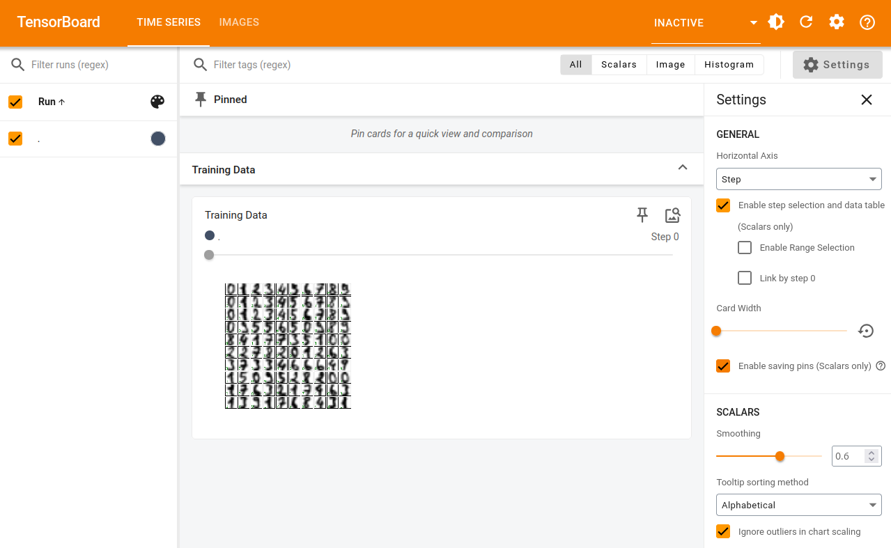"
]
},
{
"cell_type": "code",
"execution_count": 6,
"metadata": {
"id": "6jrYisoPh6TL"
},
"outputs": [],
"source": [
"from sklearn.model_selection import train_test_split\n",
"splits = train_test_split(digits.images, digits.target, random_state=0)"
]
},
{
"cell_type": "code",
"execution_count": 7,
"metadata": {
"id": "oMRcwKd4hqOo",
"outputId": "0ad36290-397b-431d-eba2-ef114daf5ea6"
},
"outputs": [
{
"name": "stdout",
"output_type": "stream",
"text": [
"images_train.shape=(1347, 8, 8) label_train.shape=(1347,)\n",
"images_test.shape=(450, 8, 8) label_test.shape=(450,)\n"
]
}
],
"source": [
"import jax.numpy as jnp\n",
"images_train, images_test, label_train, label_test = map(jnp.asarray, splits)\n",
"print(f\"{images_train.shape=} {label_train.shape=}\")\n",
"print(f\"{images_test.shape=} {label_test.shape=}\")"
]
},
{
"cell_type": "code",
"execution_count": 8,
"metadata": {
"id": "U77VMQwRjTfH",
"outputId": "345fed7a-4455-4036-85ed-57e673a4de01"
},
"outputs": [
{
"data": {
"text/html": [
"
"
],
"text/plain": [
""
]
},
"metadata": {},
"output_type": "display_data"
},
{
"data": {
"text/html": [
"
"
],
"text/plain": [
""
]
},
"metadata": {},
"output_type": "display_data"
}
],
"source": [
"from flax import nnx\n",
"\n",
"class SimpleNN(nnx.Module):\n",
"\n",
" def __init__(self, n_features: int = 64, n_hidden: int = 100, n_targets: int = 10,\n",
" *, rngs: nnx.Rngs):\n",
" self.n_features = n_features\n",
" self.layer1 = nnx.Linear(n_features, n_hidden, rngs=rngs)\n",
" self.layer2 = nnx.Linear(n_hidden, n_hidden, rngs=rngs)\n",
" self.layer3 = nnx.Linear(n_hidden, n_targets, rngs=rngs)\n",
"\n",
" def __call__(self, x):\n",
" x = x.reshape(x.shape[0], self.n_features) # Flatten images.\n",
" x = nnx.selu(self.layer1(x))\n",
" x = nnx.selu(self.layer2(x))\n",
" x = self.layer3(x)\n",
" return x\n",
"\n",
"model = SimpleNN(rngs=nnx.Rngs(0))\n",
"\n",
"nnx.display(model) # Interactive display if penzai is installed."
]
},
{
"cell_type": "markdown",
"metadata": {},
"source": [
"We've now created the basic model - the above cell will render an interactive view of the model. Which, when fully expanded, should look something like this:\n",
"\n",
""
]
},
{
"cell_type": "markdown",
"metadata": {},
"source": [
"In order to track loss across our training run, we've collected the loss function call inside the training step:"
]
},
{
"cell_type": "code",
"execution_count": 9,
"metadata": {
"id": "QwRvFPkYl5b2"
},
"outputs": [],
"source": [
"import jax\n",
"import optax\n",
"\n",
"optimizer = nnx.Optimizer(model, optax.sgd(learning_rate=0.05))\n",
"\n",
"def loss_fun(\n",
" model: nnx.Module,\n",
" data: jax.Array,\n",
" labels: jax.Array):\n",
" logits = model(data)\n",
" loss = optax.softmax_cross_entropy_with_integer_labels(\n",
" logits=logits, labels=labels\n",
" ).mean()\n",
" return loss, logits\n",
"\n",
"@nnx.jit # JIT-compile the function\n",
"def train_step(\n",
" model: nnx.Module,\n",
" optimizer: nnx.Optimizer,\n",
" data: jax.Array,\n",
" labels: jax.Array):\n",
" loss_gradient = nnx.grad(loss_fun, has_aux=True) # gradient transform!\n",
" grads, logits = loss_gradient(model, data, labels)\n",
" optimizer.update(grads) # inplace update\n",
"\n",
" # Calculate loss\n",
" loss, _ = loss_fun(model, images_test, label_test)\n",
" return loss"
]
},
{
"cell_type": "markdown",
"metadata": {},
"source": [
"Now, we've collected the metrics that were previously computed once at the end of training and called them throughout the `for` loop, as you would in an eval stage.\n",
"\n",
"With the summary_writer context in place, we write out the `Loss` scalar every epoch, test the model accuracy every 10, and stash a accuracy test sheet every 500. Any custom metric can be added this way, through the tf.summary API."
]
},
{
"cell_type": "code",
"execution_count": 10,
"metadata": {
"id": "l9mukT0eqmsr",
"outputId": "c6c7b2d6-8706-4bc3-d5a6-0396d7cfbf56"
},
"outputs": [],
"source": [
"max_epoch = 3000\n",
"with test_summary_writer.as_default():\n",
" for i in range(max_epoch):\n",
" loss = train_step(model, optimizer, images_train, label_train)\n",
" ## Store the training loss per epoch\n",
" tf.summary.scalar('Loss', loss.item(), step=i+1) #.item() because the loss coming out of train_step() is a tensor\n",
" if ((i+1)%10 == 0) or i == 0:\n",
" label_pred = model(images_test).argmax(axis=1)\n",
" num_matches = jnp.count_nonzero(label_pred == label_test)\n",
" num_total = len(label_test)\n",
" accuracy = num_matches / num_total\n",
" ## store the evaluated Accuracy every 10 epochs\n",
" tf.summary.scalar('Accuracy', accuracy.item(), step=i+1)\n",
" if ((i+1)%500 == 0) or i == 0:\n",
" fig, axes = None, None\n",
" fig, axes = plt.subplots(10, 10, figsize=(6, 6),\n",
" subplot_kw={'xticks':[], 'yticks':[]},\n",
" gridspec_kw=dict(hspace=0.1, wspace=0.1))\n",
"\n",
" label_pred = model(images_test).argmax(axis=1)\n",
"\n",
" for j, ax in enumerate(axes.flat):\n",
" ax.imshow(images_test[j], cmap='binary', interpolation='gaussian')\n",
" color = 'green' if label_pred[j] == label_test[j] else 'red'\n",
" ax.text(0.05, 0.05, str(label_pred[j]), transform=ax.transAxes, color=color)\n",
" ## store the Accuracy test sheet every 500 epochs - be sure to give each a different name, or they will overwrite the previous output.\n",
" tf.summary.image(f\"Step {i+1} Accuracy Testsheet\", plot_to_image(fig), step=i+1)"
]
},
{
"cell_type": "markdown",
"metadata": {},
"source": [
"During the training has run, and after, the added `Loss` and `Accuracy` scalars are available in the tensorboard UI under the run folder we've dynamically created by the datetime.\n",
"\n",
"The output there should look something like the following:\n",
"\n",
""
]
},
{
"cell_type": "markdown",
"metadata": {},
"source": [
"Since we've stored the example test sheet every 500 epochs, it's easy to go back and step through the progress. With each training step using all of the training data the steps and epochs are essentially the same here.\n",
"\n",
"At step 1, we see poor accuracy, as you would expect\n",
"\n",
"\n",
"\n",
"By 500, the model is essentially done, but we see the bottom row `7` get lost and recovered at higher epochs as we go far into an overfitting regime. This kind of stored data can be very useful when the training routines become automated and a human is potentially only looking when something has gone wrong.\n",
"\n",
""
]
},
{
"cell_type": "markdown",
"metadata": {},
"source": [
"Finally, it can be useful to use nnx.display's ability to visualize networks and model output. Here we feed the top 35 test images into the model and display the final output vector for each - in the top plot, each row is an individual image prediction result: each column corresponds to a class, in this case the digits (0-9). Since we're calling the highest value in a given row the class prediction (`.argmax(axis=1)`), the final image predictions (bottom plot) simply match the largest value in each row in the upper plot."
]
},
{
"cell_type": "code",
"execution_count": 11,
"metadata": {},
"outputs": [
{
"data": {
"text/html": [
"
"
],
"text/plain": [
""
]
},
"metadata": {},
"output_type": "display_data"
},
{
"data": {
"text/html": [
"
"
],
"text/plain": [
""
]
},
"metadata": {},
"output_type": "display_data"
},
{
"data": {
"text/html": [
"
"
],
"text/plain": [
""
]
},
"metadata": {},
"output_type": "display_data"
},
{
"data": {
"text/html": [
"
"
],
"text/plain": [
""
]
},
"metadata": {},
"output_type": "display_data"
},
{
"data": {
"text/plain": [
"(None, None)"
]
},
"execution_count": 11,
"metadata": {},
"output_type": "execute_result"
}
],
"source": [
"nnx.display(model(images_test[:35])), nnx.display(model(images_test[:35]).argmax(axis=1))"
]
},
{
"cell_type": "markdown",
"metadata": {},
"source": [
"The above cell output will give you an interactive plot that looks like this image below, where here we've 'clicked' in the bottom plot for entry `7` and hover over the corresponding value in the top plot.\n",
"\n",
""
]
},
{
"cell_type": "markdown",
"metadata": {},
"source": [
"## Extra Resources\n",
"\n",
"For further information about `TensorBoard` see [https://www.tensorflow.org/tensorboard/get_started](https://www.tensorflow.org/tensorboard/get_started)\n",
"\n",
"For more about `nnx.display()`, which calls Treescope under the hood, see [https://treescope.readthedocs.io/en/stable/](https://treescope.readthedocs.io/en/stable/)"
]
}
],
"metadata": {
"colab": {
"provenance": []
},
"jupytext": {
"formats": "ipynb,md:myst"
},
"kernelspec": {
"display_name": "Python 3 (ipykernel)",
"language": "python",
"name": "python3"
},
"language_info": {
"codemirror_mode": {
"name": "ipython",
"version": 3
},
"file_extension": ".py",
"mimetype": "text/x-python",
"name": "python",
"nbconvert_exporter": "python",
"pygments_lexer": "ipython3",
"version": "3.11.10"
}
},
"nbformat": 4,
"nbformat_minor": 4
}