![]()
![]() "
]
},
{
"cell_type": "markdown",
"metadata": {},
"source": [
"# Implementing PID Control in Nonlinear Simulations\n",
"\n",
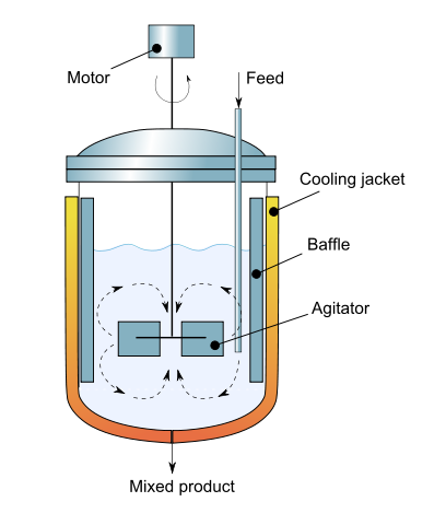
"A task common to many control projects is to simulate the PID control of a nonlinear process. This notebook demonstrates the simulation of PID for an exothermic stirred tank reactor where the objective is to control the reactor temperature through manipulation of cooling water through the reactor cooling jacket.\n",
"\n",
"\n",
"\n",
"(Diagram By [Daniele Pugliesi](http://commons.wikimedia.org/wiki/User:Daniele_Pugliesi) - Own work, [CC BY-SA 3.0](http://creativecommons.org/licenses/by-sa/3.0), [Link](https://commons.wikimedia.org/w/index.php?curid=6915706))"
]
},
{
"cell_type": "markdown",
"metadata": {},
"source": [
"## Model\n",
"\n",
"The model consists of nonlinear mole and energy balances on the contents of the well-mixed reactor.\n",
"\n",
"\\begin{align*}\n",
"V\\frac{dc}{dt} & = q(c_f - c )-Vk(T)c \\\\\n",
"\\rho C_p V\\frac{dT}{dt} & = wC_p(T_f - T) + (-\\Delta H_R)Vk(T)c + UA(T_c-T)\n",
"\\end{align*}\n",
"\n",
"where $c$ is the reactant concentration, $T$ is the reactor temperature, and $T_c$ is the cooling jacket temperature. The model is adapted from example 2.5 from Seborg, Edgar, Mellichamp and Doyle (SEMD), parameters defined and given in the table below.\n",
"\n",
"The temperature in the cooling jacket is manipulated by the cooling jacket flow, $q_c$, and governed by the energy balance\n",
"\n",
"\\begin{align*}\n",
"\\rho C_p V_c\\frac{dT_c}{dt} & = \\rho C_p q_c(T_{cf}-T_c) + UA(T - T_c)\n",
"\\end{align*}\n",
"\n",
"Normalizing the equations to isolate the time rates of change of $c$, $T$, and $T_c$ give\n",
"\n",
"\\begin{align*}\n",
"\\frac{dc}{dt} & = \\frac{q}{V}(c_f - c)- k(T)c\\\\\n",
"\\frac{dT}{dt} & = \\frac{q}{V}(T_i - T) + \\frac{-\\Delta H_R}{\\rho C_p}k(T)c + \\frac{UA}{\\rho C_pV}(T_c - T)\\\\\n",
"\\frac{dT_c}{dt} & = \\frac{q_c}{V_c}(T_{cf}-T_c) + \\frac{UA}{\\rho C_pV_c}(T - T_c)\n",
"\\end{align*}\n",
"\n",
"These are the equations that will be integrated below.\n",
"\n",
"| Quantity | Symbol | Value | Units | Comments |\n",
"| :------- | :----: | :---: | :---- | |\n",
"| Activation Energy | $E_a$ | 72,750 | J/gmol | |\n",
"| Arrehnius pre-exponential | $k_0$ | 7.2 x 10¹⁰ | 1/min | |\n",
"| Gas Constant | $R$ | 8.314 | J/gmol/K | |\n",
"| Reactor Volume | $V$ | 100 | liters | |\n",
"| Density | $\\rho$ | 1000 | g/liter | |\n",
"| Heat Capacity | $C_p$ | 0.239 | J/g/K | |\n",
"| Enthalpy of Reaction | $\\Delta H_r$ | -50,000 | J/gmol | |\n",
"| Heat Transfer Coefficient | $UA$ | 50,000 | J/min/K | |\n",
"| Feed flowrate | $q$ | 100 | liters/min | |\n",
"| Feed concentration | $c_{A,f}$ | 1.0 | gmol/liter | |\n",
"| Feed temperature | $T_f$ | 350 | K | |\n",
"| Initial concentration | $c_{A,0}$ | 0.5 | gmol/liter | |\n",
"| Initial temperature | $T_0$ | 350 | K | |\n",
"| Coolant feed temperature | $T_{cf}$ | 300 | K | |\n",
"| Nominal coolant flowrate | $q_c$ | 50 | L/min | primary manipulated variable |\n",
"| Cooling jacket volume | $V_c$ | 20 | liters | |"
]
},
{
"cell_type": "code",
"execution_count": 1,
"metadata": {
"collapsed": true
},
"outputs": [],
"source": [
"%matplotlib inline\n",
"import matplotlib.pyplot as plt\n",
"import numpy as np\n",
"from scipy.integrate import odeint\n",
"import seaborn as sns\n",
"sns.set_context('talk')\n",
"\n",
"Ea = 72750 # activation energy J/gmol\n",
"R = 8.314 # gas constant J/gmol/K\n",
"k0 = 7.2e10 # Arrhenius rate constant 1/min\n",
"V = 100.0 # Volume [L]\n",
"rho = 1000.0 # Density [g/L]\n",
"Cp = 0.239 # Heat capacity [J/g/K]\n",
"dHr = -5.0e4 # Enthalpy of reaction [J/mol]\n",
"UA = 5.0e4 # Heat transfer [J/min/K]\n",
"q = 100.0 # Flowrate [L/min]\n",
"Cf = 1.0 # Inlet feed concentration [mol/L]\n",
"Tf = 300.0 # Inlet feed temperature [K]\n",
"C0 = 0.5 # Initial concentration [mol/L]\n",
"T0 = 350.0; # Initial temperature [K]\n",
"Tcf = 300.0 # Coolant feed temperature [K]\n",
"qc = 50.0 # Nominal coolant flowrate [L/min]\n",
"Vc = 20.0 # Cooling jacket volume\n",
"\n",
"# Arrhenius rate expression\n",
"def k(T):\n",
" return k0*np.exp(-Ea/R/T)\n",
"\n",
"def deriv(X,t):\n",
" C,T,Tc = X\n",
" dC = (q/V)*(Cf - C) - k(T)*C\n",
" dT = (q/V)*(Tf - T) + (-dHr/rho/Cp)*k(T)*C + (UA/V/rho/Cp)*(Tc - T)\n",
" dTc = (qc/Vc)*(Tcf - Tc) + (UA/Vc/rho/Cp)*(T - Tc)\n",
" return [dC,dT,dTc]"
]
},
{
"cell_type": "markdown",
"metadata": {},
"source": [
"## Simulation 1. Same Initial Condition, different values of $q_c$\n",
"\n",
"The given reaction is highly exothermic. If operated without cooling, the reactor will reach an operating temperature of 500K which leads to significant pressurization, a potentially hazardous condition, and possible product degradation. \n",
"\n",
"The purpose of this first simulation is to determine the cooling water flowrate necessary to maintain the reactor temperature at an acceptable value. This simulation shows the effect of the cooling water flowrate, $q_c$, on the steady state concentration and temperature of the reactor. We use the scipy.integrate function `odeint` to create a solution of the differential equations for entire time period."
]
},
{
"cell_type": "code",
"execution_count": 2,
"metadata": {
"collapsed": true
},
"outputs": [],
"source": [
"# visualization\n",
"def plotReactor(t,X):\n",
" plt.subplot(1,2,1)\n",
" plt.plot(t,X[:,0])\n",
" plt.xlabel('Time [min]')\n",
" plt.ylabel('gmol/liter')\n",
" plt.title('Reactor Concentration')\n",
" plt.ylim(0,1)\n",
"\n",
" plt.subplot(1,2,2)\n",
" plt.plot(t,X[:,1])\n",
" plt.xlabel('Time [min]')\n",
" plt.ylabel('Kelvin');\n",
" plt.title('Reactor Temperature')\n",
" plt.ylim(300,520)"
]
},
{
"cell_type": "markdown",
"metadata": {},
"source": [
"Once the visualization code has been established, the actual simulation is straightforward."
]
},
{
"cell_type": "code",
"execution_count": 3,
"metadata": {},
"outputs": [
{
"data": {
"text/plain": [
"
"
]
},
{
"cell_type": "markdown",
"metadata": {},
"source": [
"# Implementing PID Control in Nonlinear Simulations\n",
"\n",
"A task common to many control projects is to simulate the PID control of a nonlinear process. This notebook demonstrates the simulation of PID for an exothermic stirred tank reactor where the objective is to control the reactor temperature through manipulation of cooling water through the reactor cooling jacket.\n",
"\n",
"\n",
"\n",
"(Diagram By [Daniele Pugliesi](http://commons.wikimedia.org/wiki/User:Daniele_Pugliesi) - Own work, [CC BY-SA 3.0](http://creativecommons.org/licenses/by-sa/3.0), [Link](https://commons.wikimedia.org/w/index.php?curid=6915706))"
]
},
{
"cell_type": "markdown",
"metadata": {},
"source": [
"## Model\n",
"\n",
"The model consists of nonlinear mole and energy balances on the contents of the well-mixed reactor.\n",
"\n",
"\\begin{align*}\n",
"V\\frac{dc}{dt} & = q(c_f - c )-Vk(T)c \\\\\n",
"\\rho C_p V\\frac{dT}{dt} & = wC_p(T_f - T) + (-\\Delta H_R)Vk(T)c + UA(T_c-T)\n",
"\\end{align*}\n",
"\n",
"where $c$ is the reactant concentration, $T$ is the reactor temperature, and $T_c$ is the cooling jacket temperature. The model is adapted from example 2.5 from Seborg, Edgar, Mellichamp and Doyle (SEMD), parameters defined and given in the table below.\n",
"\n",
"The temperature in the cooling jacket is manipulated by the cooling jacket flow, $q_c$, and governed by the energy balance\n",
"\n",
"\\begin{align*}\n",
"\\rho C_p V_c\\frac{dT_c}{dt} & = \\rho C_p q_c(T_{cf}-T_c) + UA(T - T_c)\n",
"\\end{align*}\n",
"\n",
"Normalizing the equations to isolate the time rates of change of $c$, $T$, and $T_c$ give\n",
"\n",
"\\begin{align*}\n",
"\\frac{dc}{dt} & = \\frac{q}{V}(c_f - c)- k(T)c\\\\\n",
"\\frac{dT}{dt} & = \\frac{q}{V}(T_i - T) + \\frac{-\\Delta H_R}{\\rho C_p}k(T)c + \\frac{UA}{\\rho C_pV}(T_c - T)\\\\\n",
"\\frac{dT_c}{dt} & = \\frac{q_c}{V_c}(T_{cf}-T_c) + \\frac{UA}{\\rho C_pV_c}(T - T_c)\n",
"\\end{align*}\n",
"\n",
"These are the equations that will be integrated below.\n",
"\n",
"| Quantity | Symbol | Value | Units | Comments |\n",
"| :------- | :----: | :---: | :---- | |\n",
"| Activation Energy | $E_a$ | 72,750 | J/gmol | |\n",
"| Arrehnius pre-exponential | $k_0$ | 7.2 x 10¹⁰ | 1/min | |\n",
"| Gas Constant | $R$ | 8.314 | J/gmol/K | |\n",
"| Reactor Volume | $V$ | 100 | liters | |\n",
"| Density | $\\rho$ | 1000 | g/liter | |\n",
"| Heat Capacity | $C_p$ | 0.239 | J/g/K | |\n",
"| Enthalpy of Reaction | $\\Delta H_r$ | -50,000 | J/gmol | |\n",
"| Heat Transfer Coefficient | $UA$ | 50,000 | J/min/K | |\n",
"| Feed flowrate | $q$ | 100 | liters/min | |\n",
"| Feed concentration | $c_{A,f}$ | 1.0 | gmol/liter | |\n",
"| Feed temperature | $T_f$ | 350 | K | |\n",
"| Initial concentration | $c_{A,0}$ | 0.5 | gmol/liter | |\n",
"| Initial temperature | $T_0$ | 350 | K | |\n",
"| Coolant feed temperature | $T_{cf}$ | 300 | K | |\n",
"| Nominal coolant flowrate | $q_c$ | 50 | L/min | primary manipulated variable |\n",
"| Cooling jacket volume | $V_c$ | 20 | liters | |"
]
},
{
"cell_type": "code",
"execution_count": 1,
"metadata": {
"collapsed": true
},
"outputs": [],
"source": [
"%matplotlib inline\n",
"import matplotlib.pyplot as plt\n",
"import numpy as np\n",
"from scipy.integrate import odeint\n",
"import seaborn as sns\n",
"sns.set_context('talk')\n",
"\n",
"Ea = 72750 # activation energy J/gmol\n",
"R = 8.314 # gas constant J/gmol/K\n",
"k0 = 7.2e10 # Arrhenius rate constant 1/min\n",
"V = 100.0 # Volume [L]\n",
"rho = 1000.0 # Density [g/L]\n",
"Cp = 0.239 # Heat capacity [J/g/K]\n",
"dHr = -5.0e4 # Enthalpy of reaction [J/mol]\n",
"UA = 5.0e4 # Heat transfer [J/min/K]\n",
"q = 100.0 # Flowrate [L/min]\n",
"Cf = 1.0 # Inlet feed concentration [mol/L]\n",
"Tf = 300.0 # Inlet feed temperature [K]\n",
"C0 = 0.5 # Initial concentration [mol/L]\n",
"T0 = 350.0; # Initial temperature [K]\n",
"Tcf = 300.0 # Coolant feed temperature [K]\n",
"qc = 50.0 # Nominal coolant flowrate [L/min]\n",
"Vc = 20.0 # Cooling jacket volume\n",
"\n",
"# Arrhenius rate expression\n",
"def k(T):\n",
" return k0*np.exp(-Ea/R/T)\n",
"\n",
"def deriv(X,t):\n",
" C,T,Tc = X\n",
" dC = (q/V)*(Cf - C) - k(T)*C\n",
" dT = (q/V)*(Tf - T) + (-dHr/rho/Cp)*k(T)*C + (UA/V/rho/Cp)*(Tc - T)\n",
" dTc = (qc/Vc)*(Tcf - Tc) + (UA/Vc/rho/Cp)*(T - Tc)\n",
" return [dC,dT,dTc]"
]
},
{
"cell_type": "markdown",
"metadata": {},
"source": [
"## Simulation 1. Same Initial Condition, different values of $q_c$\n",
"\n",
"The given reaction is highly exothermic. If operated without cooling, the reactor will reach an operating temperature of 500K which leads to significant pressurization, a potentially hazardous condition, and possible product degradation. \n",
"\n",
"The purpose of this first simulation is to determine the cooling water flowrate necessary to maintain the reactor temperature at an acceptable value. This simulation shows the effect of the cooling water flowrate, $q_c$, on the steady state concentration and temperature of the reactor. We use the scipy.integrate function `odeint` to create a solution of the differential equations for entire time period."
]
},
{
"cell_type": "code",
"execution_count": 2,
"metadata": {
"collapsed": true
},
"outputs": [],
"source": [
"# visualization\n",
"def plotReactor(t,X):\n",
" plt.subplot(1,2,1)\n",
" plt.plot(t,X[:,0])\n",
" plt.xlabel('Time [min]')\n",
" plt.ylabel('gmol/liter')\n",
" plt.title('Reactor Concentration')\n",
" plt.ylim(0,1)\n",
"\n",
" plt.subplot(1,2,2)\n",
" plt.plot(t,X[:,1])\n",
" plt.xlabel('Time [min]')\n",
" plt.ylabel('Kelvin');\n",
" plt.title('Reactor Temperature')\n",
" plt.ylim(300,520)"
]
},
{
"cell_type": "markdown",
"metadata": {},
"source": [
"Once the visualization code has been established, the actual simulation is straightforward."
]
},
{
"cell_type": "code",
"execution_count": 3,
"metadata": {},
"outputs": [
{
"data": {
"text/plain": [
"![]()
![]() "
]
}
],
"metadata": {
"kernelspec": {
"display_name": "Python 3",
"language": "python",
"name": "python3"
},
"language_info": {
"codemirror_mode": {
"name": "ipython",
"version": 3
},
"file_extension": ".py",
"mimetype": "text/x-python",
"name": "python",
"nbconvert_exporter": "python",
"pygments_lexer": "ipython3",
"version": "3.7.4"
},
"widgets": {
"state": {
"0593fc1c63274b289c5fff97127efb4d": {
"views": [
{
"cell_index": 15
}
]
}
},
"version": "1.2.0"
}
},
"nbformat": 4,
"nbformat_minor": 2
}
"
]
}
],
"metadata": {
"kernelspec": {
"display_name": "Python 3",
"language": "python",
"name": "python3"
},
"language_info": {
"codemirror_mode": {
"name": "ipython",
"version": 3
},
"file_extension": ".py",
"mimetype": "text/x-python",
"name": "python",
"nbconvert_exporter": "python",
"pygments_lexer": "ipython3",
"version": "3.7.4"
},
"widgets": {
"state": {
"0593fc1c63274b289c5fff97127efb4d": {
"views": [
{
"cell_index": 15
}
]
}
},
"version": "1.2.0"
}
},
"nbformat": 4,
"nbformat_minor": 2
}