![]()
![]() "
]
},
{
"cell_type": "markdown",
"metadata": {
"colab_type": "text",
"id": "HedPhu1-uqXL"
},
"source": [
"# Log-Optimal Growth and the Kelly Criterion"
]
},
{
"cell_type": "markdown",
"metadata": {
"colab_type": "text",
"id": "Jc08h8eGuqXL"
},
"source": [
"This [IPython notebook](http://ipython.org/notebook.html) demonstrates the Kelly criterion and other phenomena associated with log-optimal growth."
]
},
{
"cell_type": "markdown",
"metadata": {
"colab_type": "text",
"id": "LN9Xm4q0uqXM"
},
"source": [
"## Initializations"
]
},
{
"cell_type": "code",
"execution_count": null,
"metadata": {
"colab": {},
"colab_type": "code",
"id": "udCWC5J-uqXN"
},
"outputs": [],
"source": [
"%matplotlib notebook\n",
"\n",
"import matplotlib.pyplot as plt\n",
"import numpy as np\n",
"import random"
]
},
{
"cell_type": "markdown",
"metadata": {
"colab_type": "text",
"id": "ui0RvOnxuqXQ"
},
"source": [
"## What are the Issues in Managing for Optimal Growth?"
]
},
{
"cell_type": "markdown",
"metadata": {
"colab_type": "text",
"id": "Y0tFvIxuuqXQ"
},
"source": [
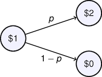
"Consider a continuing 'investment opportunity' for which, at each stage, an invested dollar will yield either two dollars with probability $p$ or nothing with probability $1-p$. You can think of this as a gambling game if you like, or as sequence of business investment decisions.\n",
"\n",
"\n",
"\n",
"Let $W_k$ be the wealth after $k$ stages in this sequence of decisions. At each stage $k$ there will be an associated return $R_k$ so that\n",
"\n",
"$$W_k = R_k W_{k-1}$$\n",
"\n",
"Starting with a wealth $W_0$, after $k$ stages our wealth will be\n",
"\n",
"$$W_k = R_kR_{k-1}\\cdots R_2R_1W_0$$\n",
"\n",
"Now let's consider a specific investment strategy. To avoid risking total loss of wealth in a single stage, we'll consider a strategy where we invest a fraction $\\alpha$ of our remaining wealth, and retain a fraction $1-\\alpha$ for future use. Under this strategy, the return $R_k$ is given by\n",
"\n",
"$$R_k = \\begin{cases} 1+\\alpha & \\mbox{with probability}\\quad p \\\\ 1-\\alpha & \\mbox{with probability}\\quad 1-p\\end{cases}$$\n",
"\n",
"How should we pick $\\alpha$? A small value means that wealth will grow slowly. A large value will risk more of our wealth in each trial."
]
},
{
"cell_type": "markdown",
"metadata": {
"colab_type": "text",
"id": "d4wl2IfsuqXR"
},
"source": [
"## Why Maximizing Expected Wealth is a Bad Idea"
]
},
{
"cell_type": "markdown",
"metadata": {
"colab_type": "text",
"id": "e7ioaVPZuqXS"
},
"source": [
"At first glance, maximizing expected wealth seems like a reasonable investment objective. Suppose after $k$ stages we have witnessed $u$ profitable outcomes (i.e., 'wins'), and $k-u$ outcomes showing a loss. The remaining wealth will be given by\n",
"\n",
"$$W_k/W_0 = (1+\\alpha)^u(1-\\alpha)^{k-u}$$\n",
"\n",
"The binomial distribution gives the probability of observing $u$ 'wins' in $k$ trials\n",
"\n",
"$$Pr(u \\mbox{ wins in } k \\mbox{ trials}) = {k\\choose{u}}p^u (1-p)^{k-u}$$\n",
"\n",
"So the expected value of $W_k$ is given by\n",
"\n",
"$$E[W_k/W_0] = \\sum_{u=0}^{k} {k\\choose{u}}p^u (1-p)^{k-u}(1+\\alpha)^u(1-\\alpha)^{k-u}$$\n",
"\n",
"Next we plot $E[W_k/W_0]$ as a function of $\\alpha$. If you run this notebook on your own server, you can adjust $p$ and $K$ to see the impact of changing parameters."
]
},
{
"cell_type": "code",
"execution_count": null,
"metadata": {
"colab": {},
"colab_type": "code",
"id": "BUbFBBUfuqXT",
"outputId": "6128296e-5fc4-4e68-b45f-64db1c9b3eaa"
},
"outputs": [
{
"data": {
"application/vnd.jupyter.widget-view+json": {
"model_id": "90f394624e7448e6a425e2f5a18ad4ee"
}
},
"metadata": {
"tags": []
},
"output_type": "display_data"
}
],
"source": [
"from scipy.misc import comb\n",
"from ipywidgets import interact\n",
"\n",
"def sim(K = 40,p = 0.55):\n",
" alpha = np.linspace(0,1,100)\n",
" W = [sum([comb(K,u)*((p*(1+a))**u)*(((1-p)*(1-a))**(K-u)) \\\n",
" for u in range(0,K+1)]) for a in alpha]\n",
" plt.figure()\n",
" plt.plot(alpha,W,'b')\n",
" plt.xlabel('alpha')\n",
" plt.ylabel('E[W({:d})/W(0)]'.format(K))\n",
" plt.title('Expected Wealth after {:d} trials'.format(K))\n",
"\n",
"interact(sim,K=(1,60),p=(0.4,0.6,0.01));"
]
},
{
"cell_type": "markdown",
"metadata": {
"colab_type": "text",
"id": "Po0g0gTIuqXY"
},
"source": [
"This simulation suggests that if each stage is, on average, a winning proposition with $p > 0.5$, then expected wealth after $K$ stages is maximized by setting $\\alpha = 1$. This is a very risky strategy. \n",
"\n",
"To show how risky, the following cell simulates the behavior of this process for as a function of $\\alpha$, $p$, and $K$. Try different values of $\\alpha$ in the range from 0 to 1 to see what happens."
]
},
{
"cell_type": "code",
"execution_count": null,
"metadata": {
"colab": {},
"colab_type": "code",
"id": "tlVMPSGmuqXZ",
"outputId": "91df71c7-75e6-4e01-9cec-dbdf9cec4abd"
},
"outputs": [
{
"data": {
"application/vnd.jupyter.widget-view+json": {
"model_id": "00de5525a9e84114a4d03dcd75f5468d"
}
},
"metadata": {
"tags": []
},
"output_type": "display_data"
},
{
"data": {
"text/plain": [
"
"
]
},
{
"cell_type": "markdown",
"metadata": {
"colab_type": "text",
"id": "HedPhu1-uqXL"
},
"source": [
"# Log-Optimal Growth and the Kelly Criterion"
]
},
{
"cell_type": "markdown",
"metadata": {
"colab_type": "text",
"id": "Jc08h8eGuqXL"
},
"source": [
"This [IPython notebook](http://ipython.org/notebook.html) demonstrates the Kelly criterion and other phenomena associated with log-optimal growth."
]
},
{
"cell_type": "markdown",
"metadata": {
"colab_type": "text",
"id": "LN9Xm4q0uqXM"
},
"source": [
"## Initializations"
]
},
{
"cell_type": "code",
"execution_count": null,
"metadata": {
"colab": {},
"colab_type": "code",
"id": "udCWC5J-uqXN"
},
"outputs": [],
"source": [
"%matplotlib notebook\n",
"\n",
"import matplotlib.pyplot as plt\n",
"import numpy as np\n",
"import random"
]
},
{
"cell_type": "markdown",
"metadata": {
"colab_type": "text",
"id": "ui0RvOnxuqXQ"
},
"source": [
"## What are the Issues in Managing for Optimal Growth?"
]
},
{
"cell_type": "markdown",
"metadata": {
"colab_type": "text",
"id": "Y0tFvIxuuqXQ"
},
"source": [
"Consider a continuing 'investment opportunity' for which, at each stage, an invested dollar will yield either two dollars with probability $p$ or nothing with probability $1-p$. You can think of this as a gambling game if you like, or as sequence of business investment decisions.\n",
"\n",
"\n",
"\n",
"Let $W_k$ be the wealth after $k$ stages in this sequence of decisions. At each stage $k$ there will be an associated return $R_k$ so that\n",
"\n",
"$$W_k = R_k W_{k-1}$$\n",
"\n",
"Starting with a wealth $W_0$, after $k$ stages our wealth will be\n",
"\n",
"$$W_k = R_kR_{k-1}\\cdots R_2R_1W_0$$\n",
"\n",
"Now let's consider a specific investment strategy. To avoid risking total loss of wealth in a single stage, we'll consider a strategy where we invest a fraction $\\alpha$ of our remaining wealth, and retain a fraction $1-\\alpha$ for future use. Under this strategy, the return $R_k$ is given by\n",
"\n",
"$$R_k = \\begin{cases} 1+\\alpha & \\mbox{with probability}\\quad p \\\\ 1-\\alpha & \\mbox{with probability}\\quad 1-p\\end{cases}$$\n",
"\n",
"How should we pick $\\alpha$? A small value means that wealth will grow slowly. A large value will risk more of our wealth in each trial."
]
},
{
"cell_type": "markdown",
"metadata": {
"colab_type": "text",
"id": "d4wl2IfsuqXR"
},
"source": [
"## Why Maximizing Expected Wealth is a Bad Idea"
]
},
{
"cell_type": "markdown",
"metadata": {
"colab_type": "text",
"id": "e7ioaVPZuqXS"
},
"source": [
"At first glance, maximizing expected wealth seems like a reasonable investment objective. Suppose after $k$ stages we have witnessed $u$ profitable outcomes (i.e., 'wins'), and $k-u$ outcomes showing a loss. The remaining wealth will be given by\n",
"\n",
"$$W_k/W_0 = (1+\\alpha)^u(1-\\alpha)^{k-u}$$\n",
"\n",
"The binomial distribution gives the probability of observing $u$ 'wins' in $k$ trials\n",
"\n",
"$$Pr(u \\mbox{ wins in } k \\mbox{ trials}) = {k\\choose{u}}p^u (1-p)^{k-u}$$\n",
"\n",
"So the expected value of $W_k$ is given by\n",
"\n",
"$$E[W_k/W_0] = \\sum_{u=0}^{k} {k\\choose{u}}p^u (1-p)^{k-u}(1+\\alpha)^u(1-\\alpha)^{k-u}$$\n",
"\n",
"Next we plot $E[W_k/W_0]$ as a function of $\\alpha$. If you run this notebook on your own server, you can adjust $p$ and $K$ to see the impact of changing parameters."
]
},
{
"cell_type": "code",
"execution_count": null,
"metadata": {
"colab": {},
"colab_type": "code",
"id": "BUbFBBUfuqXT",
"outputId": "6128296e-5fc4-4e68-b45f-64db1c9b3eaa"
},
"outputs": [
{
"data": {
"application/vnd.jupyter.widget-view+json": {
"model_id": "90f394624e7448e6a425e2f5a18ad4ee"
}
},
"metadata": {
"tags": []
},
"output_type": "display_data"
}
],
"source": [
"from scipy.misc import comb\n",
"from ipywidgets import interact\n",
"\n",
"def sim(K = 40,p = 0.55):\n",
" alpha = np.linspace(0,1,100)\n",
" W = [sum([comb(K,u)*((p*(1+a))**u)*(((1-p)*(1-a))**(K-u)) \\\n",
" for u in range(0,K+1)]) for a in alpha]\n",
" plt.figure()\n",
" plt.plot(alpha,W,'b')\n",
" plt.xlabel('alpha')\n",
" plt.ylabel('E[W({:d})/W(0)]'.format(K))\n",
" plt.title('Expected Wealth after {:d} trials'.format(K))\n",
"\n",
"interact(sim,K=(1,60),p=(0.4,0.6,0.01));"
]
},
{
"cell_type": "markdown",
"metadata": {
"colab_type": "text",
"id": "Po0g0gTIuqXY"
},
"source": [
"This simulation suggests that if each stage is, on average, a winning proposition with $p > 0.5$, then expected wealth after $K$ stages is maximized by setting $\\alpha = 1$. This is a very risky strategy. \n",
"\n",
"To show how risky, the following cell simulates the behavior of this process for as a function of $\\alpha$, $p$, and $K$. Try different values of $\\alpha$ in the range from 0 to 1 to see what happens."
]
},
{
"cell_type": "code",
"execution_count": null,
"metadata": {
"colab": {},
"colab_type": "code",
"id": "tlVMPSGmuqXZ",
"outputId": "91df71c7-75e6-4e01-9cec-dbdf9cec4abd"
},
"outputs": [
{
"data": {
"application/vnd.jupyter.widget-view+json": {
"model_id": "00de5525a9e84114a4d03dcd75f5468d"
}
},
"metadata": {
"tags": []
},
"output_type": "display_data"
},
{
"data": {
"text/plain": [
"![]()
![]() "
]
}
],
"metadata": {
"colab": {
"collapsed_sections": [],
"name": "07.08-Log-Optimal-Growth-and-the-Kelly-Criterion.ipynb",
"provenance": [],
"version": "0.3.2"
},
"kernelspec": {
"display_name": "Python 3",
"language": "python",
"name": "python3"
},
"language_info": {
"codemirror_mode": {
"name": "ipython",
"version": 3
},
"file_extension": ".py",
"mimetype": "text/x-python",
"name": "python",
"nbconvert_exporter": "python",
"pygments_lexer": "ipython3",
"version": "3.7.3"
}
},
"nbformat": 4,
"nbformat_minor": 2
}
"
]
}
],
"metadata": {
"colab": {
"collapsed_sections": [],
"name": "07.08-Log-Optimal-Growth-and-the-Kelly-Criterion.ipynb",
"provenance": [],
"version": "0.3.2"
},
"kernelspec": {
"display_name": "Python 3",
"language": "python",
"name": "python3"
},
"language_info": {
"codemirror_mode": {
"name": "ipython",
"version": 3
},
"file_extension": ".py",
"mimetype": "text/x-python",
"name": "python",
"nbconvert_exporter": "python",
"pygments_lexer": "ipython3",
"version": "3.7.3"
}
},
"nbformat": 4,
"nbformat_minor": 2
}