k-Wave Toolbox

Loading External Image Maps Example

Overview

This example demonstrates how to assign an external image to the initial pressure distribution for the simulation of an initial value problem within a two-dimensional homogeneous propagation medium. It builds on the Homogeneous Propagation Medium Example.

• open the file in the MATLAB Editor
• run the file in MATLAB

 Back to Top

Loading the image map

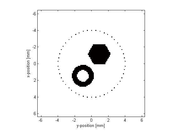
The initial pressure distribution source.p0 used by kspaceFirstOrder2D is simply a two-dimensional matrix filled with arbitrary numeric values. Consequently, any data may be used to define this distribution. Here an external image map is loaded using loadImage. This function converts an external image into a matrix, sums the colour channels (for colour images), and scales the pixel values from 0 to 1.

% load the initial pressure distribution from an image and scale the
% magnitude
p0_magnitude = 3;
p0 = p0_magnitude*loadImage('EXAMPLE_source_one.png');

The medium discretisation is again performed by calling makeGrid with the required grid dimensions, after which resize is used to scale the loaded image map to the required dimensions.

% create the computational grid
Nx = 128;           % number of grid points in the x (row) direction
Ny = 128;           % number of grid points in the y (column) direction
dx = 0.1e-3;        % grid point spacing in the x direction  [m]
dy = 0.1e-3;        % grid point spacing in the y direction  [m]
kgrid = makeGrid(Nx, dx, Ny, dy);

% resize the image to match the size of the computational grid and assign
% to the source input structure
source.p0 = resize(p0, [Nx, Ny]);

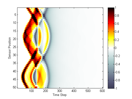
The simulation is invoked in the same way as in the previous examples. A plot of the initial pressure distribution and sensor mask, and a visualisation of the recorded pressure field are shown below.

 Back to Top

Defining A Sensor Mask By Opposing Corners

Heterogeneous Propagation Medium

© 2009-2014 Bradley Treeby and Ben Cox.