k-Wave Toolbox

Iterative Image Improvement Using Time Reversal Example

Overview

This example demonstrates how photoacoustic image reconstruction may be improved iteratively. First, the sensor data is simulated using kspaceFirstOrder2D. Then, in the first reconstruction, an image is formed from data recorded on a line array using time reversal. In the second, an image is formed from data recorded on an L-shaped sensor array (also using time reversal). In the final stage, this image is improved iteratively. This example builds on the 2D Time Reversal Reconstruction For A Line Sensor Example.

• open the file in the MATLAB Editor
• run the file in MATLAB

 Back to Top

Simulating the sensor data

The example begins by defining an initial pressure distribution using a pre-defined image of the word 'k-Wave'.

% load an image for the initial pressure distribution
p0_image = loadImage('k-Wave.png');

% make it binary
p0_image = (p0_image>0);

% smooth and scale the initial pressure distribution
p0_magnitude = 2;
p0 = p0_magnitude*smooth(kgrid, p0_image, true);

% assign to the source structure
source.p0 = p0;   

The acoustic pressure time series that would be measured at each of the sensors in an L-shaped sensor array are then simulated using kspaceFirstOrder2D.

 Back to Top

Reconstruction using data from a line array

Part of this data - for those sensors forming a line array - is then used in a time reversal image reconstruction, just as in the 2D Time Reversal Reconstruction For A Line Sensor Example.

% define a line array of sensors
sensor.mask = zeros(Nx, Ny);
sensor.mask(1, :) = 1;

% assign the time reversal data
sensor.time_reversal_boundary_data = sensor_data((sensor.mask(original_sensor_indices) == 1),:);

% set the initial pressure to be zero
source.p0 = 0;

% run the time reversal reconstruction
p0_line = kspaceFirstOrder2D(kgrid, medium, source, sensor, input_args{:});

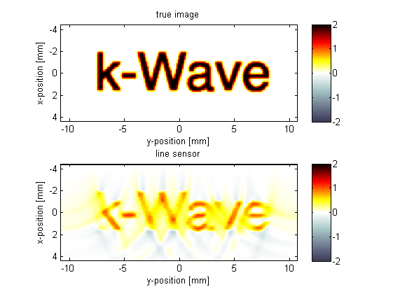
The initial pressure distribution and image resulting from this first reconstruction are shown below:

 Back to Top

Reconstruction using data from an L-shaped array

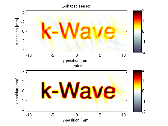
The image reconstruction is then repeated using all the data measured over the L-shaped array.

% extend the array to the original L-shaped form
sensor.mask(:, 1) = 1;

% assign the time reversal data
sensor.time_reversal_boundary_data = sensor_data;

% run the time reversal reconstruction
p0_L = kspaceFirstOrder2D(kgrid, medium, source, sensor, input_args{:});

The image is noticeably improved, but can be improved further still by iterating, which is described below.

 Back to Top

Iteratively improving the image reconstruction

Beginning with the image obtained from the L-shaped sensor, an iterative procedure is now used to improve it. This improvement is achieved by adding an additional set of (imaginary) sensors so that the sensor array encloses the region of interest. The missing data for these 'sensors' is then estimated using the forward model with the best image obtained so far. (In fact, a non-negativity condition is applied to the image before it is used in the forward model, as we know that in photoacoustics the initial pressure distribution cannot be negative.) The original data and the estimated data are then used together to form an image, which - at least within the region satisfying the visibility (audibility) condition - will be an improvement on the previous image. The estimate of the missing data and subsequent image reconstruction may then be iterated for even greater image improvement.

Niterations = 5;
for loop = 1:Niterations
    % apply a non-negativity condition 
    source.p0 = p0_iterated.*(p0_iterated>=0);

    % set the sensor mask to be just the missing sides of the box
    sensor.mask = zeros(Nx, Ny);
    sensor.mask(end, :) = 1;
    sensor.mask(:,end) = 1;

    %remove the time-reversed field so the forward model will run
    sensor = rmfield(sensor,'time_reversal_boundary_data');

    % estimate the data on the missing sides of the box
    estimated_sensor_data = kspaceFirstOrder2D(kgrid, medium, source, sensor, input_args{:});

    % define the full box array
    sensor.mask = zeros(Nx, Ny);
    sensor.mask(1,:) = 1;
    sensor.mask(:,1) = 1;
    sensor.mask(end,:) = 1;
    sensor.mask(:,end) = 1;

    %combine the measured data with the newly estimated data
    combined_sensor_data = zeros(sum(sensor.mask(:)==1),kgrid.Nt);
    combined_sensor_data(sensor_box_indices1,:) = estimated_sensor_data;
    combined_sensor_data(sensor_box_indices2,:) = sensor_data;

    % assign the time reversal data
    sensor.time_reversal_boundary_data = combined_sensor_data;    

    % reset the initial pressure
    source.p0 = 0;

    % run the time reversal reconstruction
    p0_iterated = kspaceFirstOrder2D(kgrid, medium, source, sensor, input_args{:});
end

The images from the non-iterated and iterated reconstructions using the data from the L-shaped array are shown above. Notice that within the region in which the visibility condition is satisfied (ie. the normals to every boundary in the image within this region cross the measurement surface somewhere) the image is recovered well, but outside this region there remain artefacts. That is inevitable and cannot be improved without recording more data (or perhaps making other a priori assumptions).

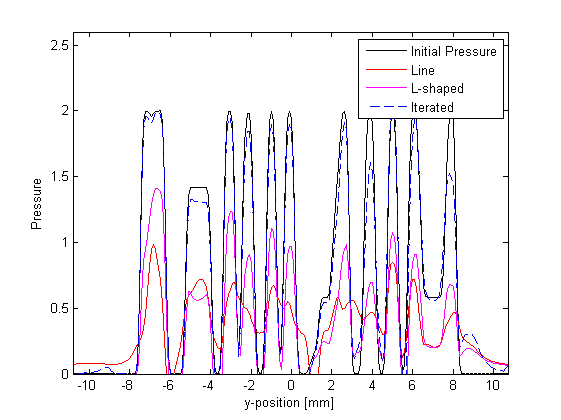
To show that the accuracy of the amplitudes is significantly improved, a horizontal profile through the centre of the image is shown below for the various reconstructions.

 Back to Top

Image Reconstruction With Bandlimited Sensors

Attenuation Compensation Using Time Reversal

© 2009-2014 Bradley Treeby and Ben Cox.