k-Wave Toolbox

Modelling Sensor Directivity in 2D Example

Overview

This example demonstrates how the sensitivity of a large single element detector varies with the angular position of a point-like source. It builds on Monopole Point Source In A Homogeneous Propagation Medium and Focussed Detector in 2D examples.

• open the file in the MATLAB Editor
• run the file in MATLAB

 Back to Top

Defining a large element detector

The sensor is defined as a binary sensor mask in the shape of a line.

% define a large area detector 
sensor.mask = zeros(Nx, Ny);
sensor.mask(Nx/2+1, (Ny/2-9):(Ny/2+11)) = 1;

 Back to Top

Defining a collection of point sources

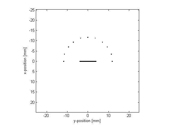
Equi-spaced point sources are then defined at a fixed distance from the centre of the detector face. To do this, the Cartesian coordinates of the source points are calculated using makeCartCircle. A binary source mask corresponding to these Cartesian points is then calculated using cart2grid. The indices of the matrix elements for which the binary mask is equal to 1 (the source points) are found using find.

% define equally spaced point sources lying on a circle centred at the
% centre of the detector face 
circle = makeCartCircle(30*dx, 11, [0, 0], pi);

% find the binary sensor mask most closely corresponding to the cartesian
% points coordinates from makeCartCircle
circle = cart2grid(kgrid,circle);

% find the indices of the sources in the binary source mask
source_positions = find(circle == 1);

A time varying pressure source is defined to drive the point sources.

% define a time varying sinusoidal source
source_freq = 0.25e6;
source_mag = 1;
source.p = source_mag*sin(2*pi*source_freq*kgrid.t_array);

% filter the source to remove high frequencies not supported by the grid
source.p = filterTimeSeries(kgrid, medium, source.p);

 Back to Top

Running simulations for each point source

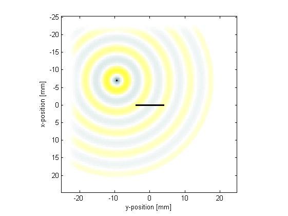
For each point source, a new binary source mask is defined, and the simulation is run. When each simulation has finished, the returned sensor data is summed together to mimic a single large detector.

for source_loop = 1:length(source_positions)
    
    % select a point source
    source.p_mask = zeros(Nx, Ny);
    source.p_mask(source_positions(source_loop)) = 1;

    % create a display mask to display the transducer
    display_mask = source.p_mask + sensor.mask;

    % run the simulation
    input_args = {'DisplayMask', display_mask, 'PlotScale', [-0.5 0.5]};
    sensor_data = kspaceFirstOrder2D(kgrid, medium, source, sensor, input_args{:});

    % average the data recorded for each grid point to simulate the
    % measured signal from a large aperture, single element, detector
    single_element_data(:, source_loop) = sum(sensor_data, 1);

end

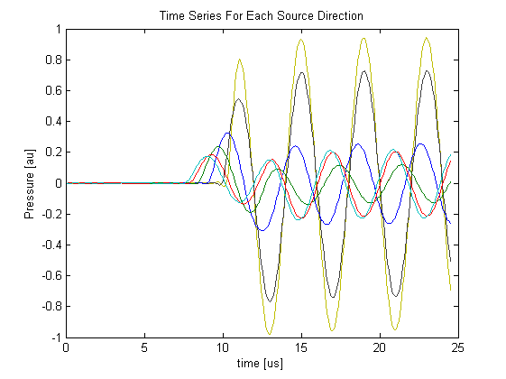
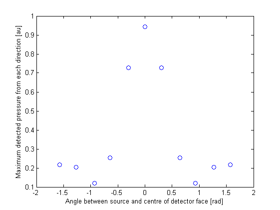
The recorded time series corresponding to the different source positions are plotted below. The maximum of each time series are also plotted as a function of angle, where the angle is defined between the detector plane and a line joining the point source and the centre of the detector face. The directionality introduced by the large size of the detector is clearly seen.

 Back to Top

Focussed Detector in 3D

Modelling Sensor Directivity in 3D

© 2009-2014 Bradley Treeby and Ben Cox.