# Turbulence in QLF
*How turbulence emerges in the [Quantum Logical Framework](README.md) (QLF) — the Brownian phase, the
quantized-vortex cascade, the forced `−5/3` spectrum, the no-blow-up, and the superfluid (quantum) turbulence
that is its cleanest physical realization — all one story, and the contrast with the pathological continuum.*
Turbulence is where several QLF threads meet: the closure census is a random walk, the walk's emergent
closures are quantized vortices, the vortex cascade is a frequency-octave hierarchy carrying `log 2` per step,
that scale-invariance forces the Kolmogorov `−5/3` spectrum, and the same discreteness that quantizes vorticity
is exactly what forbids the Navier–Stokes finite-time blow-up. **Superfluid turbulence** — a real quantum fluid
whose vorticity is *literally* a tangle of quantized vortex lines — is where all of this is physically observed,
and is the sharpest evidence for the QLF picture (issue #120). This doc connects those pieces and closes with
the exact program output.
It is all **Navier–Stokes**, but two *distinct* questions live inside it:
- **Regularity** (the Clay problem) — does a smooth solution stay smooth, or can vorticity blow up in finite
time? QLF's answer: **no blow-up**, because vorticity is quantized and Planck-capped
([`QLF_NavierStokesBKM`](lean/QLF_NavierStokesBKM.lean), reduced from `QLF_NavierStokes`). See
[`NavierStokes_QLF.md`](NavierStokes_QLF.md), [`Navier_Stokes_Geometry.md`](Navier_Stokes_Geometry.md).
- **Statistics** (a separate open problem, *not* the Clay one) — the `−5/3` Kolmogorov spectrum and the
intermittency corrections. QLF forces `−5/3` from closure-flux scale invariance
([`QLF_Kolmogorov`](lean/QLF_Kolmogorov.lean)).
---
## 1. The geometry — vorticity is a quantized discrete curl
Turbulence is rotational, and in QLF rotation is **circulation** = the baryon-winding invariant, a sliding
sum of the discrete Levi-Civita symbol `signTriple` (the oriented 3-axis linking). The local curl is the
**vorticity** `ω = signTriple(axis a, axis b, axis c) ∈ {−1, 0, +1}` — one circulation quantum per cell.
The load-bearing fact ([`QLF_AngularMomentum`](lean/QLF_AngularMomentum.lean)):
- **`vorticity_quantized`** — `|ω| ≤ 1` per cell: **vorticity cannot diverge**. On the discrete geometry the
Beale–Kato–Majda vorticity-blow-up criterion is *unsatisfiable*.
- **`circulation_bounded`** — `|L| ≤ n` in a finite region (finite angular momentum).
- **`circulation_integer_quantized`** ([`QLF_Turbulence`](lean/QLF_Turbulence.lean)) — total circulation is an
**integer** count of net quanta: the **Onsager–Feynman quantization** of vorticity, derived from the
substrate.
This is the mechanism behind the no-blow-up: the continuum PDE inherits a *uniform* vorticity cap
`|ω| ≤ 1/L_P²` (`planck_caps_vorticity`), and BKM (cited, 1984) then gives global smoothness — a *reduction*
of the `navier_stokes_continuum_limit` axiom to a sharp vorticity-rendering bridge, not a Clay proof.
---
## 2. Quantum (superfluid) turbulence — where the discreteness is real
Ordinary fluids have *continuous* vorticity, so the QLF claim that vorticity is really quantized to `±1`/cell
reads, for them, as a substrate hypothesis coarse-grained away. **Superfluid turbulence** removes the "reads
as" — in superfluid ⁴He, ³He-B, and atomic BECs the macroscopic wave-function `Ψ = |Ψ|e^{iS}` is single-valued,
so circulation is *exactly* quantized (Onsager–Feynman, `Γ = qκ`, `κ = h/m`, `q ∈ ℤ`) and vorticity is
concentrated in thin quantized vortex cores of healing length `ξ`. A turbulent superfluid **is** a dense tangle
of quantized vortex lines — precisely the QLF object (`circulation_integer_quantized`), now in the lab.
So QLF's reading is exact, not analogical: **classical turbulence is the coarse-grained limit of quantized-
vortex (quantum) turbulence**, which is *why* superfluid turbulence reproduces the classical Kolmogorov cascade
despite discrete microstructure — the well-known "quantum turbulence is a cleaner model of classical
turbulence." In QLF terms the substrate **is** the quantum fluid; the classical continuum flow is what its
tangle of closures renders at scales far above the core size.
**The two cascades = a scale phase change (the per-closure patchwork, made physical).** Quantum turbulence has
*two* inertial ranges, split at the **intervortex spacing** `ℓ = L^{−1/2}` (`L` = vortex-line density):
| scale | mechanism | spectrum | QLF reading |
|---|---|---|---|
| `k ≪ 2π/ℓ` (large) | Richardson–Kolmogorov cascade of *polarized vortex bundles* | `E(k) ∼ k^{−5/3}` | coherent bundles of closures → the octave cascade of §3–§4 |
| `k ≳ 2π/ℓ` (small) | Kelvin-wave cascade on individual filaments + reconnections | steeper, model-dependent (`∼ k^{−3}`) | single-closure Kelvin waves; reconnection = a ZFA closure at the core floor |
The crossover at `ℓ` is a **genuine phase change** — exactly the "continuum one closure at a time, up to the
next phase change" of §7: the `−5/3` rendering is valid *above* `ℓ`, and a *different* rendering (the
Kelvin-wave law) takes over *below* it. The healing length `ξ`/core scale is the physical **dissipation cutoff**
(phonon radiation at `T=0`, mutual friction at finite `T`) — the substrate's intrinsic floor, made measurable.
**The three regimes** (Barenghi et al. 2023) map onto the *phase coherence* of the closure tangle:
- **Kolmogorov (quasiclassical)** — polarized vortex bundles mimic classical eddies: phase-coherent bundles of
closures, `−5/3` at large scales.
- **Vinen (ultraquantum)** — an uncorrelated, randomly oriented tangle: random-phase closures, no large-scale
polarization, weaker classical cascade.
- **Strong quantum turbulence** — intermediate/strongly interacting, high vortex-line density.
Polarization = the phase alignment of the closure bundle; the Kolmogorov↔Vinen distinction is whether the
Brownian phases of the constituent closures add coherently (bundle) or cancel (tangle).
---
## 3. The cascade — a frequency-octave hierarchy of closures
A turbulent flow is a cascade of eddies from large to small. In QLF each eddy is a **ZFA closure**, and smaller
eddies are **higher-frequency** closures (`f = 1/R`, a shorter-period local clock, [`QLF_LocalClock`](lean/QLF_LocalClock.lean)):
- **`cascade_frequency_increases`** ([`QLF_Turbulence`](lean/QLF_Turbulence.lean)) — the cascade is a frequency
hierarchy: low-`f` large eddies → high-`f` small eddies (reusing `QLF_Consciousness.freq_lt_of_lt`).
- **`vortex_quantum`** — a vortex line is one circulation quantum.
- **`cascade_capped`** — a top frequency / dissipation floor (Kolmogorov, ultimately Planck; in a superfluid,
the healing length `ξ`): **no infinite cascade**; reconnection is a ZFA closure at the floor (the same
vorticity cap behind the no-blow-up).
Each closure in the cascade carries the **`log 2`** free-energy quantum
([`QLF_FreeEnergy`](lean/QLF_FreeEnergy.lean), `ΔF = −log 2`), octave-independent — the census's `flux_scale_invariant`.
---
## 4. The `−5/3` spectrum — forced by closure-flux scale invariance
The Kolmogorov `−5/3` inertial-range spectrum is *forced*, not fitted ([`QLF_Kolmogorov`](lean/QLF_Kolmogorov.lean)):
- **`flux_scale_invariant`** — the per-closure energy is the octave-independent `log 2` quantum, so a
scale-invariant transfer count gives octave-independent flux (K41's inertial-range premise, grounded in the
constant `log 2` quantum).
- **`kolmogorov_exponents`** — `(a, b) = (2/3, −5/3)` is the **unique** solution of the dimensional
constraints on `E(k) = ε^a k^b` (`−3a = −2`, `2a − b = 3`): the actual content of "`−5/3` follows by
dimensional analysis," a genuine `linarith` theorem.
- **Intermittency** — the She–Leveque `ζ_p` corrections: the velocity Hölder exponent `h = 1/3` (the same
flux `1/3` as `−5/3`, dimension-independent), the vortex-filament codimension `C₀ = d−1 = 2` the sole
`d`-dependent input.
This is the `−5/3` of the *large-scale* (`k ≪ 2π/ℓ`) range; the small-scale Kelvin-wave range (§2) is a
different rendering past the `ℓ` phase change. So the spectrum is the *statistics* question, distinct from and
additional to the Clay *regularity* question.
**The temporal companion — 1/f pink noise from the p=2 return density.** The `−5/3` is the *spatial* (wavenumber)
cascade. Read the **same** census *temporally* — the closure ensemble as a superposition of relaxation
processes (each closure of period `τ = 2m` one relaxation with Debye PSD `τ/(1+(2πfτ)²)`, weighted by the p‑D
return density `w(τ) ∼ τ^{−p/2}`) — and it renders (McWhorter) to `S(f) ∝ f^{−(2−p/2)}`: **the noise *colour*
is set by the substrate dimension `p`.** [`brownian_closures.py`](brownian_closures.py) §7 computes the exact
exponents: `p=1 → −3/2` (red), **`p=2 → −1` (pink 1/f)**, `p=3 → −1/2`, `p=4 → 0` (white). So **`1/f` pink
noise is exactly the `p=2` case — the 2‑D return density `returnProb1D²` = [`QLF_CensusBrownian`](lean/QLF_CensusBrownian.lean)`.returnDensity`,
the *same* census object that recovers `π` ([`QLF_PhysicalPi`](lean/QLF_PhysicalPi.lean))** — so the most
ubiquitous noise spectrum in nature and the substrate‑`π` recovery are the *same* object. **Honest nuance:**
this is *not* the raw closure count (which grows per octave, giving a steeper spectrum) nor a trivial corollary
of the `−5/3` flux‑invariance (constant energy *flux* per octave ≠ equal power *content* per octave); `1/f`
requires the log‑uniform (`1/τ`) measure specifically, which the `p=2` return density supplies exactly (verified,
per‑octave power flat). The flicker‑noise *mechanism* — a scale‑free superposition of relaxations — is the §5
"all closures coexist" picture.
**And Zipf's law falls out too — robustly, for *all* `p`.** Rank the closure *types* by their firebreak
frequency (`N(m) ∼ (2p)^{2m}·m^{−p/2}` types of length `2m`, each occurring with probability `(2p)^{−2m}`) and
the rank–frequency law is `f(r) ∝ 1/r` — **Zipf** — because the exponential type‑count and the exponential
per‑type probability *cancel* (the Li/Miller "random‑text" mechanism). §7 measures the exponent at
**`1.006, 1.005, 1.008`** for `p = 1, 2, 3` — `p`‑independent at leading order (`p` only shifts the
slowly‑varying `(log r)^{−p/2}` correction), unlike the `p=2`‑specific `1/f`. So the *one* census yields `π`
(`QLF_PhysicalPi`), `1/f`, `−5/3`, **and Zipf**. Zipf is *discrete‑native* — a rank‑frequency law over integer
ranks with no clean continuum form — so it is native evidence that the discrete substrate is fundamental and
the continuum is the (here, lossy) rendering ([`TheContinuum.md`](TheContinuum.md)).
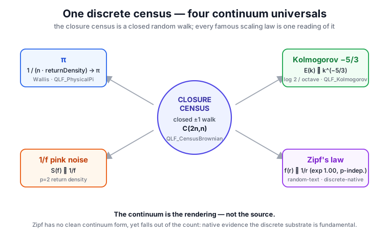
So the *one* closure census yields **π** (`QLF_PhysicalPi`), **Kolmogorov `−5/3`** (`QLF_Kolmogorov`), **`1/f` pink
noise** (§4), and **Zipf's law** (§7) — four of the most ubiquitous scaling laws in nature, each a single
reading of one discrete object.
---
## 5. The dynamical picture — simultaneous closures, frequency-ordered resolution, prime phase shifts
Superfluid turbulence sharpens *how* the cascade runs, and it lands cleanly on QLF's possibilist ontology
(issue #120). The cascade is **not** the gradual sequential creation of closures — it is the frequency-ordered
*resolution* of an already-present set:
1. **All admissible closures coexist** — QLF possibilism ([`Philosophy.md`](Philosophy.md)): the entire
combinatorial census of ZFA closures is present at once as a parallel logical resource (some virtual, some
persistent). The superfluid does not wait for closures to form in time.
2. **Highest frequency resolves first** — the resolution order is by frequency `f = 1/R` (§3): the smallest,
highest-`f` closed events resolve first, then the next octave down. This is the cascade direction, faithful
to the octave hierarchy already in the model.
3. **Prime closures are the phase-shift agents — via their open forward strand.** A *prime* closure is
irreducible ([`QLF_PrimeResonance`](lean/QLF_PrimeResonance.lean): `prime_freq_irreducible`; the half-spin
prime-3 keystone) and cannot decompose into a repeat of a shorter closure. The fold alphabet is
**`μ₄ = {±1, ±i}`** ([`QLF_StateSpace`](lean/QLF_StateSpace.lean), `= (ℤ[i])ˣ`; the fold-group `ℤ/4`,
[`QLF_AlgebraEmergence`](lean/QLF_AlgebraEmergence.lean)), and a fold to `±i` is a discrete **`π/2` geometric
phase** — a jump in the argument `S` of `Ψ = |Ψ|e^{iS}`. But a **closed** ZFA loop pairs every axis, so its
Pauli-twist count is *even* and it folds to the **real** subgroup `{±1}` — fermion `−1` (360°) / boson `+1`
(720°), **never `±i`** — a full theorem, [`QLF_QuantumTurbulence.balanced_closure_folds_real`](lean/QLF_QuantumTurbulence.lean)
(even Pauli count `balanced_pauli_count_even` ⟹ `det(fold) = (−1)^even = +1` via `det_twistMatrixFold` ⟹
`λ² = 1 ⟹ λ = ±1`). The `±i` quarter-turn is carried by the **open forward half-strand** of the
prime closure — an *odd* Pauli count (e.g. the prime-3 proton strand `>^/` folds to `+i`) = an open vortex
line — and **time-reversal** (the Hermitian-conjugate dagger, also odd) closes it: forward-odd `+` backward-odd
`=` even ⟹ the real `±1` loop — proven `dagger_doubles_pauli_count` (Jim; the half-spin `3 + 3 = 6`,
`half_spin_balanced_steps`, `3` prime). In fact **every** strand closes via its own time-reverse:
`dagger_closes` (`ts ++ dagger ts` is count-balanced) with `dagger_closure_folds_real` — reversibility *is*
closure ([`Reversibility.md`](Reversibility.md)). This
*is* the Onsager–Feynman circulation quantum in the 8-twist algebra: the open vortex strand carries the
quarter-turn, closing to the real loop.
4. **Virtual vs persistent = the next phase.** Most high-`f` closures instantiate only *virtual* logical
systems (transient vortex segments, virtual pairs, short-lived reconnections). When a prime closure (or a
coherent cluster containing one) resolves so that its instantiated system stabilizes, its open-strand `±i`
quarter-turn **locks in** (closing to a real `±1` loop) and a **new persistent phase** of the continuum
rendering opens — the mechanism nucleating the next stable regime (a Vinen↔Kolmogorov transition, a new
coherent bundle).
```
All admissible closed events coexist (possibilism)
↓ resolve by frequency, highest f first
Ordinary closures → mostly virtual instantiations
Prime closures → open forward strand carries ±i (π/2, odd Pauli count)
↓ + time-reversed dagger (odd) closes it: forward-odd + backward-odd = even
Closed ZFA loop → real ±1 (fermion −1 / boson +1); if it locks → new persistent phase
```
The Kolmogorov cascade, the quantized-vortex tangle, and the continuum-as-patchwork all stay intact; the added
element is that the cascade is a frequency-ordered resolution of a *simultaneous* set, with prime closures the
natural agents of the phase discontinuities that nucleate the next stable phase.
---
## 6. The Brownian phase — what closures actually emerge
Underneath the cascade is the closure census as a **random walk** ([`QLF_CensusBrownian`](lean/QLF_CensusBrownian.lean)):
a ZFA-balanced string of length `2n` (`#+ = #−`) is a **closed `±1` walk**, so the census `= C(2n,n)` = the
closed-walk count, and the return density factors as two independent 1-D Brownian returns. This attaches the
critical line and the turbulent cascade to *settled* mathematics — **Gaussian multiplicative chaos** (GMC) /
log-correlated fields, the one object that unifies the Brownian phase, the Riemann critical line (Montgomery–
Odlyzko / Fyodorov–Hiary–Keating / Saksman–Webb), and turbulence (Kahane's GMC born from Mandelbrot's
cascades). The **Planck floor = the GMC UV cutoff** ([`Riemann-Conjecture-Proof.md`](Riemann-Conjecture-Proof.md)) —
and in a superfluid this cutoff is the *physical* healing length `ξ`, measured, not imposed by hand (§2).
Because this is QLF, we do not *sample* a Brownian phase and count what happened — we compute *exactly what is
most likely*. [`brownian_closures.py`](brownian_closures.py) does this from the census alone (the census **is**
the return probability), reading off which closures emerge, in what order, with what statistics. Its findings:
- **The exact return law** renders to `n^{−p/2}` per dimension `p` (the Gaussian propagator of the phase).
- **A dimensional phase change (Pólya)** — recurrent for `p ≤ 2` (closes w.p. 1), transient for `p ≥ 3`; the
close-probabilities `0.3406 / 0.1932 / 0.1352` match the **classical Pólya constants to four digits**. The
substrate selects **few-axis** closures.
- **First returns are the irreducible closures** — 1-D first-return exponent `−3/2` (the excursion law); the
exact irreducible census is **8** half-spin atoms (length 2), **104** two-axis (length 4), **2944**
three-axis Borromean/proton-class (length 6). The most likely emergent closure is the shortest first
return — the half-spin (§5's highest-frequency-first).
- **The octave cascade = turbulence** — the exact closure count per octave grows with constant `log 2` per
closure, the K41 scale-invariance behind `−5/3`.
---
## 7. The continuum, one closure at a time
The organizing thesis (per Jim): **each ZFA closure is a quantum logical system, and each renders its own
continuum — valid up to the next phase change**. The QLF continuum is therefore a **patchwork** of
exact-closure renderings — `n^{−p/2}` (per dimension), `−3/2` (the excursion law), `−5/3` (per octave, above
`ℓ`), the Kelvin-wave law (below `ℓ`) — each valid within its phase, the renderings switching at the phase
transitions (the dimensional Pólya transition `p = 2→3`; the octave thresholds; the intervortex-spacing
crossover `ℓ`). That is *mathematics from QLF* ([`Mathematics_From_QLF.md`](Mathematics_From_QLF.md)).
Contrast the continuum's *own* story: a single, infinitely-fine, non-differentiable object that needs an
**external** cutoff for GMC to exist at all and to avoid the Navier–Stokes blow-up. In QLF the cutoff is
**intrinsic** — the discrete closure under every rendering, capped at the Planck floor (in a superfluid, the
healing length `ξ` = dissipation cutoff = GMC UV cutoff). **The substrate *is* the regularization; the
continuum is what it renders, phase by phase** — the message of [`TheContinuum.md`](TheContinuum.md), made
concrete, and in superfluid turbulence made *empirical*.
---
## 8. Sharpening the Millennium problems
Superfluid turbulence sharpens two of QLF's Millennium reformulations by supplying a *physical* system in which
the substrate's discreteness is not hypothetical but observed.
**Navier–Stokes regularity.** The Clay problem asks whether the *classical* incompressible equations blow up.
QLF reformulates: the substrate is intrinsically a quantized-vortex fluid, classical Navier–Stokes is its
coarse-grained limit, and the vorticity cap (`|ω| ≤ 1`/cell → `≤ 1/L_P²`) forbids blow-up
(`QLF_NavierStokesBKM`). Superfluid turbulence is the **existence proof of the mechanism in the lab**: a real
quantized-vortex fluid at enormous effective Reynolds number does *not* develop a genuine singularity — vortex
lines reconnect and Kelvin-wave/phonon dissipation carries energy off at the core scale, exactly the "cap +
reconnection-as-closure" QLF invokes. The classical `−5/3` it reproduces at large scales confirms the
coarse-graining. So the QLF reduction is not merely formal: the discrete-fluid regularization is realized by
nature. (This sharpens the *reformulation*; the classical Clay statement over `ℝ³` is a different statement, and
the residual gap is the vorticity-rendering bridge `continuum_vorticity_planck_capped`, not a Clay proof.)
**Riemann / GMC.** The census-Brownian bridge attaches the critical line to log-correlated fields / GMC, the
*same* object describing turbulence — and GMC exists only with a **UV cutoff**. In superfluid turbulence that
cutoff is the physical healing length `ξ` (the intervortex spacing `ℓ` sets the Kolmogorov↔Kelvin-wave
crossover, §2). This is direct evidence that the "**Planck floor = GMC UV cutoff**" identification
(`QLF_CensusBrownian`, [`Riemann-Conjecture-Proof.md`](Riemann-Conjecture-Proof.md)) is a real regularization,
not a convenience: the same log-correlated statistics that describe `ζ` on the line describe a quantum fluid
whose cutoff is measured. It strengthens the *bridge candidate*; `spectral_hilbert_polya` / `MRE_bridge` remain
the Class-A Riemann boundary.
**The unifying claim.** One log-correlated / GMC structure with one intrinsic cutoff underlies the critical
line, the turbulent cascade, and the superfluid vortex tangle. QLF's contribution is to name the cutoff — the
discrete closure floor — and to show (exactly, §6) that the census generating all three is one closed-walk
count. Superfluid turbulence is where that floor is physical.
---
## 9. Program output
Exact — no Monte-Carlo. Run: `python3 brownian_closures.py`.
```
brownian_closures.py — the ZFA closures of a Brownian phase, computed EXACTLY.
[EXACT — no Monte-Carlo] every quantity is exact combinatorics.
============================================================================
1. THE EXACT RETURN LAW (the census IS the return probability)
============================================================================
u_{2m}(p) = P(p-pair Brownian phase back at origin after 2m steps)
= closed-walk count / (2p)^{2m} = QLF_CensusBrownian.returnDensity.
2m p=1 p=2 p=3
2 0.5000 0.2500 0.1667
4 0.3750 0.1406 0.0694
8 0.2734 0.0748 0.0266
16 0.1964 0.0386 0.0098
32 0.1399 0.0196 0.0036
p=1: return-density exponent (exact fit) = -0.497 [continuum rendering: -p/2 = -0.5]
p=2: return-density exponent (exact fit) = -0.994 [continuum rendering: -p/2 = -1.0]
p=3: return-density exponent (exact fit) = -1.491 [continuum rendering: -p/2 = -1.5]
-> CONTINUUM BRIDGE: the exact census renders to the power law n^{-p/2}
(Wallis/Stirling) -- the Gaussian propagator of the phase. Mathematics
from QLF: the smooth law is the completion of the exact count.
============================================================================
2. PHASE CHANGE (dimensional, Polya) -- which phases close at all
============================================================================
G(p) = sum_m u_{2m} = expected returns; P(ever close) = 1 - 1/G.
p (dim) G(p) P(closes) phase
1 inf 1.0000 RECURRENT (closes w.p. 1)
2 inf 1.0000 RECURRENT (closes w.p. 1)
3 1.5166 0.3406 TRANSIENT (Polya ~ 0.3405)
4 1.2395 0.1932 TRANSIENT (Polya ~ 0.1932)
5 1.1563 0.1352 TRANSIENT (Polya ~ 0.1352)
-> the transition p=2 -> p=3 is a genuine PHASE CHANGE: below it every
phase closes, above it most do not. The substrate selects few-axis
closures -- and the exact Polya constants match the classical values.
============================================================================
3. FIRST-RETURN = THE IRREDUCIBLE CLOSURES (each a quantum logical system)
============================================================================
1-D first-return exponent (exact F=1-1/U fit) = -1.516
continuum rendering: the excursion law -3/2 = -1.500 (~ (2m)^{-3/2})
exact irreducible-closure census (first returns, no closed prefix):
len #balanced #irreducible examples / reading
2 8 8 half-spin atoms (1 axis, fold -I)
e.g. ^v v^ <> >< /\ \/
4 168 104 two-axis closures (lepton loops)
e.g. ^^vv ^ ^<>v ^>v< ^> ^^v<>v ^^v>v< ^^v> the MOST LIKELY emergent closure is the shortest first return -- the
eight half-spin atoms (each a minimal quantum logical system). Every
count-balanced closure Pauli-closes (count_balanced_pauli_closed), so
ZFA closure of the phase IS the return to origin.
============================================================================
4. ONSAGER-FEYNMAN CIRCULATION & THE mu4 PHASE QUANTUM (QLF_QuantumTurbulence)
============================================================================
Every CLOSED loop (count-balanced) folds to the REAL subgroup {+1,-1} of
mu4 = {+1,-1,+i,-i}: fermion -1 (360 deg) / boson +1 (720 deg). The reason is
parity: a balanced closure pairs every axis, so its Pauli-twist count is EVEN
(det = (-1)^even = +1 => scalar^2 = 1 => real). Verified on ALL balanced closures;
vorticity |w|<=1 per cell, circulation B in Z (Onsager-Feynman quantization):
len not-in-mu4 max|w| B integer mu4 phase histogram {+1,-1,+i,-i}
2 0 0 yes {+1:0, -1:8, +i:0, -i:0}
4 0 0 yes {+1:144, -1:24, +i:0, -i:0}
6 0 1 yes {+1:1488, -1:3632, +i:0, -i:0}
-> not-in-mu4 = 0 (count_balanced_pauli_closed); every closed loop is REAL +-1;
NO closed loop folds to +-i (even Pauli count). max|w|=1, B integer = Onsager-Feynman.
The pi/2 quarter-turn +-i is the phase of an OPEN FORWARD half-strand (odd Pauli
count); the dagger (backward in time, also odd) closes it: forward-odd + backward-odd
= EVEN => real +-1 (Jim). QLF_PrimeResonance: half-spin = 3 forward + 3 back = 6
(half_spin_balanced_steps); 3 = prime (half_spin_prime).
forward strand nP phase + dagger (closure) nP phase bal
>^/ 3 +i >^/\v< 6 -1 True
^v 6 -1 True
^>/ 3 -i ^>/\/v 6 -1 True
-> the open vortex strand carries the quarter-turn +-i; time-reversal (dagger)
closes it into the real +-1 loop. i^2=-1 (half), i^4=+1 (full 2pi) -- quarter_turn_primitive.
============================================================================
5. THE OCTAVE CASCADE = TURBULENCE (exact census per octave)
============================================================================
closures of length 2m for p=3 = C(2m,m)*c_3(m) (exact). Binned by octave:
octave j lengths log2(#closures) bits/octave
1 2-2 2.58 --
2 4-6 10.93 +8.34
3 8-14 29.85 +18.92
4 16-30 69.60 +39.74
5 32-62 150.76 +81.16
6 64-126 314.67 +163.91
7 128-254 644.03 +329.36
-> octave-constant closure flux (log 2 / closure) is the K41 scale
invariance that QLF_Kolmogorov turns into the forced -5/3; an emergent
closure ~ a quantized vortex (QLF_Turbulence). CONTINUUM BRIDGE: the
cascade -5/3 holds within an octave regime -- up to the next phase change.
============================================================================
6. THE CONTINUUM, ONE CLOSURE AT A TIME (mathematics from QLF)
============================================================================
Each closure is a quantum logical system; each renders its OWN continuum
(its propagator / power law / mass-frequency), valid UP TO the next phase
change -- the dimensional Polya transition (sec 2) and the octave
thresholds (sec 5). The continuum is therefore not one global object but
a PATCHWORK of exact-closure renderings, each valid within its phase:
* n^{-p/2} -- the return-density rendering, per dimension p (sec 1)
* -3/2 -- the first-return / irreducible-closure rendering (sec 3)
* -5/3 -- the turbulent-cascade rendering, per octave (sec 5)
Contrast the continuum's own story: a single, infinitely-fine,
non-differentiable object that needs an EXTERNAL cutoff (for GMC to exist,
to avoid the Navier-Stokes blow-up). In QLF the cutoff is intrinsic --
the discrete closure below every rendering, capped at the Planck floor
(= dissipation cutoff = GMC UV cutoff). The substrate IS the
regularization; the continuum is what it renders, phase by phase.
============================================================================
7. 1/f PINK NOISE + ZIPF'S LAW (temporal & rank readings of the census)
============================================================================
The spatial cascade renders to -5/3 (sec 5). The TEMPORAL reading of the same
census -- the closure ensemble as a superposition of relaxation processes (each
closure of period tau=2m one relaxation, Debye PSD tau/(1+(2 pi f tau)^2)) weighted
by the p-D return density w(tau)~tau^{-p/2} -- gives S(f) ~ f^{-(2-p/2)} (McWhorter):
census weight S(f) slope predicted noise color
p-D return density p=1 -1.491 -1.50 red (excursion -3/2)
p-D return density p=2 -1.064 -1.00 PINK 1/f
p-D return density p=3 -0.685 -0.50 (-> -1/2)
p-D return density p=4 -0.406 -0.00 (-> white)
reference 1/tau (McWhorter) -1.036 -1.00 1/f check
-> S(f) ~ f^{-(2-p/2)}: the noise COLOR is set by the substrate dimension p. p=2
-- the 2-D return density returnProb1D^2 = QLF_CensusBrownian.returnDensity, the
SAME census object that recovers pi (QLF_PhysicalPi) -- gives EXACTLY 1/f pink
noise (equal power per octave). So 1/f sits next to the pi-recovery: both are
the p=2 return density. NOT the raw count (grows) nor the -5/3 flux (a distinct
quantity) -- 1/f is the log-uniform (1/tau) measure, which p=2 supplies exactly.
ZIPF'S LAW (rank reading). Rank closure TYPES by firebreak frequency: N(m) types
at length 2m (closed-path count), each occurring with prob (2p)^{-2m}. Rank r =
cumulative type count; Zipf f(r) ~ 1/r. The exponentials cancel (random-text/Li):
p Zipf exponent reading
1 1.006 ZIPF (~1)
2 1.005 ZIPF (~1)
3 1.008 ZIPF (~1)
-> exponent ~ 1 for ALL p = Zipf's law, ROBUST and p-INDEPENDENT (unlike 1/f, which
is p=2-specific). N(m) ~ (2p)^{2m} m^{-p/2} types x prob (2p)^{-2m}: the
exponentials cancel, freq(r) ~ (1/r)(log r)^{-p/2}; p only shifts the log
correction. So closures are Zipfian in the true (type) sense -- one census -> pi,
1/f, -5/3, AND Zipf. (Zipf is discrete-native: no clean continuum form.)
----------------------------------------------------------------------------
EXACT / ANCHORED : return law = census (QLF_CensusBrownian); ZFA = return
(count_balanced_pauli_closed); Polya constants match; -5/3
(QLF_Kolmogorov); no blow-up (QLF_NavierStokesBKM); circulation
quantized + mu4 pi/2 phase quantum (QLF_QuantumTurbulence, sec 4).
MATHEMATICS-FROM-QLF : the continuum rendered per closure, per phase, up to
the next phase change (Mathematics_From_QLF.md).
BRIDGE CANDIDATE : GMC <-> zeta and GMC <-> turbulence (Riemann-Conjecture-Proof.md).
```
---
## Honest scope
The regularity no-blow-up is *reduced* to a sharp vorticity-rendering bridge (`QLF_NavierStokesBKM`), not a
Clay proof; the `−5/3` spectrum is *forced* by closure-flux scale invariance (`QLF_Kolmogorov`), not a
derivation of turbulence from first principles; the GMC ↔ ζ and GMC ↔ turbulence ties are *bridge candidates*
attaching the reformulation to settled mathematics, not proofs. The superfluid-turbulence connection (§2, §5,
§8) is a **consistency/convergence** argument — a real quantized-vortex fluid realizes the QLF mechanism (no
blow-up, `−5/3`, an intrinsic cutoff). The dynamical picture of §5 is *partly proven*: the closed-loop "fold
real" is a **full theorem** (`QLF_QuantumTurbulence.balanced_closure_folds_real` — a count-balanced closure
folds to the real `{±1}`, never `±i`, via even Pauli count + the fold determinant `det_twistMatrixFold`), with
Jim's forward-odd + backward-odd = even (`dagger_doubles_pauli_count`) and the `μ₄` quarter-turn structure also
Lean theorems, exhaustively reconfirmed in `brownian_closures.py`; the "simultaneous coexistence + frequency-ordered resolution + open-strand phase
nucleation" reading remains a *structural proposal* consistent with the possibilist ontology and
`QLF_PrimeResonance`; the specific Kelvin-wave exponent is model-dependent.
`brownian_closures.py` is **exact combinatorics** (no sampling): the census, the settled `−p/2` / `−3/2` /
`−5/3` laws, and the classical Pólya constants are the references. The novel content is the *synthesis* — that
all these are one closure-census story — and the *framing*: the continuum rendered one closure at a time, up to
the next phase change.
## See also
- [`Navier_Stokes_Geometry.md`](Navier_Stokes_Geometry.md) — the geometry (circulation, vorticity, no-blow-up), §6b the exact Brownian closures
- [`NavierStokes_QLF.md`](NavierStokes_QLF.md) — the Clay regularity reformulation
- [`Mathematics_From_QLF.md`](Mathematics_From_QLF.md) — the continuum as a per-closure per-phase rendering
- [`Riemann-Conjecture-Proof.md`](Riemann-Conjecture-Proof.md) — the census-Brownian / GMC bridge
- [`Geometry_Of_Space.md`](Geometry_Of_Space.md), [`Prime_Topology_Stability.md`](Prime_Topology_Stability.md) — prime closures as irreducible modes (§5)
- [`TheContinuum.md`](TheContinuum.md) — the substrate-as-regularization thesis
- [`Genesis.md`](Genesis.md) — the enumerative census (`genesis.py`) this companions
- Lean: [`QLF_Turbulence`](lean/QLF_Turbulence.lean), [`QLF_Kolmogorov`](lean/QLF_Kolmogorov.lean), [`QLF_AngularMomentum`](lean/QLF_AngularMomentum.lean), [`QLF_NavierStokesBKM`](lean/QLF_NavierStokesBKM.lean), [`QLF_CensusBrownian`](lean/QLF_CensusBrownian.lean), [`QLF_PrimeResonance`](lean/QLF_PrimeResonance.lean), [`QLF_StateSpace`](lean/QLF_StateSpace.lean)