# exploreRGEE
The goal of exploreRGEE is to explore Google Earth Engine (GEE) in the
Rstudio IDE. This package uses bindings and functions from
[rgee](https://github.com/r-spatial/rgee) and other spatial packages
([sf](https://github.com/r-spatial/sf),
[leaflet](https://github.com/rstudio/leaflet)) to explore Google Earth
Engine collections relatively quickly while using R. This package is
meant to be exploratory and experimental but also provides the user
quick functions to reproducible tasks, e.g. repetitive workflows. The
reason for doing this in R is that some people are not familiar with
JavaScript or Python but versed in R and this provides easy access to
use GEE with commonly used methods for exploratory data analysis
([tidyverse](https://github.com/tidyverse/tidyverse)).
## Installation
Development version from [GitHub](https://github.com/) with:
``` r
# install.packages("devtools")
devtools::install_github("joshualerickson/exploreRGEE")
# recommended
# https://github.com/mikejohnson51/AOI/tree/master/R
remotes::install_github("mikejohnson51/AOI")
```
## Important Note
The backbone of this package relies on
[rgee](https://github.com/r-spatial/rgee) and a GEE account (it’s free),
so for more information go to the rgee
[website](https://github.com/r-spatial/rgee) or the GEE
[website](https://developers.google.com/earth-engine/) for more details
on how to get set-up and also tons of functionality using the
[rgee](https://github.com/r-spatial/rgee) package!
## Similar Packages
Here is a list of similar packages that I’ve come across. Please let me
know of any more!
[rgee](https://github.com/r-spatial/rgee)
[eemont](https://github.com/davemlz/eemont)
[earthEngineGrabR](https://jesjehle.github.io/earthEngineGrabR/)
[geemap](https://github.com/giswqs/geemap)
## Flow
The main flow of exploreRGEE is to **get** GEE data and then either
vizualize (`viz()`), reduce regions (`rr()`) or look at time series
(`band()`). For example,
``` r
get_*() %>% viz()
get_*() %>% rr()
get_*() %>% band()
```
## Development
Contributions are welcome!
## Example
This is a basic example which shows you how to solve a common problem:
visualizing net annual NPP data and creating a time series.
``` r
library(exploreRGEE)
library(rgee)
library(AOI)
#this initializes the API
ee_Initialize()
#> -- rgee 1.0.8.9999 ---------------------------------- earthengine-api 0.1.249 --
#> v email: not_defined
#> v Initializing Google Earth Engine: v Initializing Google Earth Engine: DONE!
#> v Earth Engine user: users/joshualerickson
#> --------------------------------------------------------------------------------
```
Let’s look at Northwestern Montana and the median NPP over a 30 year
span (1986 to 2016). To do this, we’ll call the `get_npp()`. This `gets`
the collection while doing some pre-processing steps, e.g. date range,
cloud masking, etc. You could also just use the `get_any()` function and
provide the appropriate arguments.
``` r
lincoln_county <- AOI::aoi_get(state = "Montana", county = "Lincoln")
npp <- get_npp(lincoln_county, method = 'ld_NPP', param = 'annualNPP', stat = 'median', startDate = '1986-01-01', endDate = '2016-01-01')
```
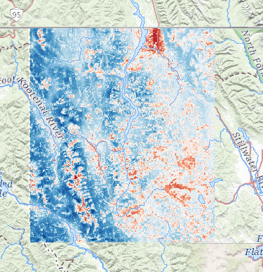
Now we can vizualize this Image with `viz()`. The scale argument in this
function is a way to get a *close* guess at a min/max argument. If you
already have an idea of a min/max value (e.g. Normalized Difference:
0-1) then just put that into the arguments and `viz()` will not run
`getInfo()`. This approach makes visualising much faster.
``` r
npp %>% viz(scale = 250)
```
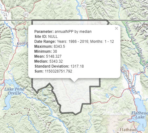
Ok, now that we’ve got an idea of the area let’s see what it would
look like if we reduced this area of interest. To do that we’ll use the
`rr()` function. This function uses any GEE Feature Collection or sf
object to reduce regions to common statistics, e.g. mean, max, min,
median, stdDev and sum. **Scale** matters in this situation! So, make
sure you understand what the underlying scale is. Sometimes I’ll use a
big scale just to see a coarse depiction and then when I go to the
analyis I’ll reduce that scale, up the `tileScale` and run
`lazy = TRUE`.
``` r
npp %>% rr(scale = 250, leaflet = TRUE)
```
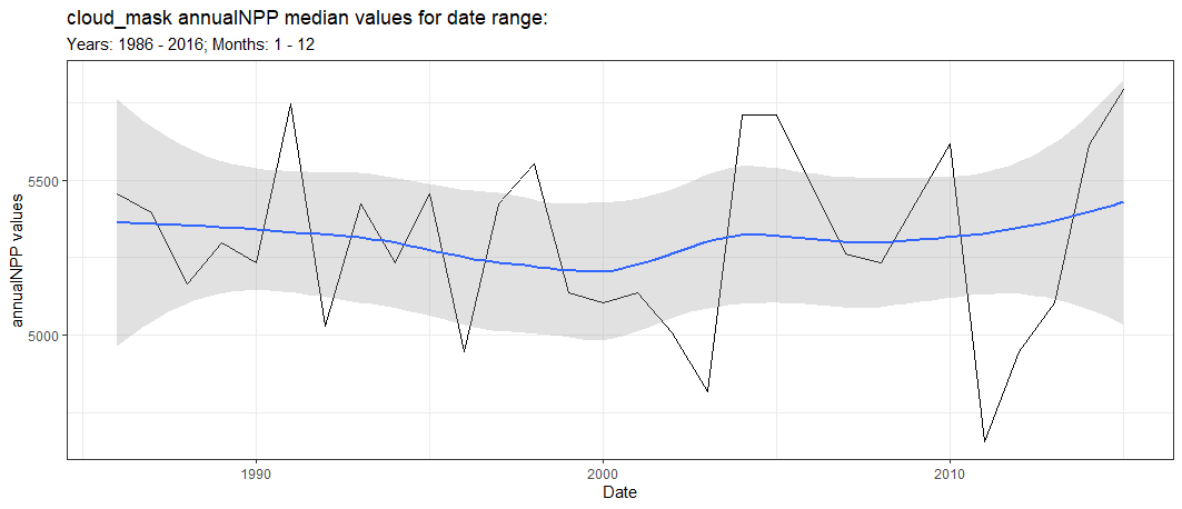
Maybe we want to see how this region looked over time and not as
static statistics? Well, we can use the `band()` function to do this.
This function takes each year and `toBands()` the ImageCollection. From
there, using rgee `ee_extract()` we can then convert to table values.
This is an expensive function and you can use `lazy = TRUE`. This will
split the object into 10 groups and run a for loop in the background in
sequential. Future developments will hopefully make this parallel.
``` r
npp %>% band(scale = 1000, ggplot = TRUE)
```