Continuous TSP Formulation

Kalvik Jakkala

I developed a formulation for the Travelling Salesperson Problem. The problem considers a set of nodes, each of which needs to be visited so that the total distance traveled is minimized. The problem often arises in path planning when multiple locations of interest have to be visited. One can use the method developed here to generate either a tour or a path. Moreover, we can modify the technique to include constraints to use a specific node as either the start or end node to visit. However, the implementation below only generates paths where the algorithm decides the start and end nodes. Additionally, we can use the method to solve a problem of any size, but the optimality of the solution it converges is not studied yet.

Most TSP solvers are based on discrete operations and usually utilize greedy heuristics to find sub-optimal solutions. However, I hypothesized that we could solve the problem by formulating the problem as a continuous optimization problem and using gradient descent to find its optimal. The formulation presented is continuous and fully differentiable. Moreover, it's global optimal would indeed coincide with the optimal solution of the TSP problem. However, the optimization landscape is relatively large, and finding such an optimal is difficult with first-order solvers such as gradient descent. As such, the method is likely to get stuck in a local optimal.

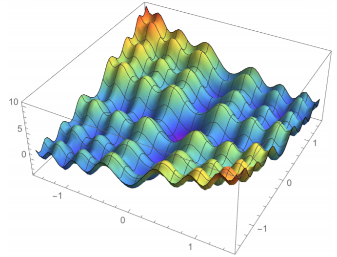
I believe the optimization landscape looks like the one shown below. Given the abundance of local minima, stochastic gradient descent is not well suited to solve the problem. Moreover, I don't think higher-order optimization methods will do any good either, as they won't necessarily look past the local valley.

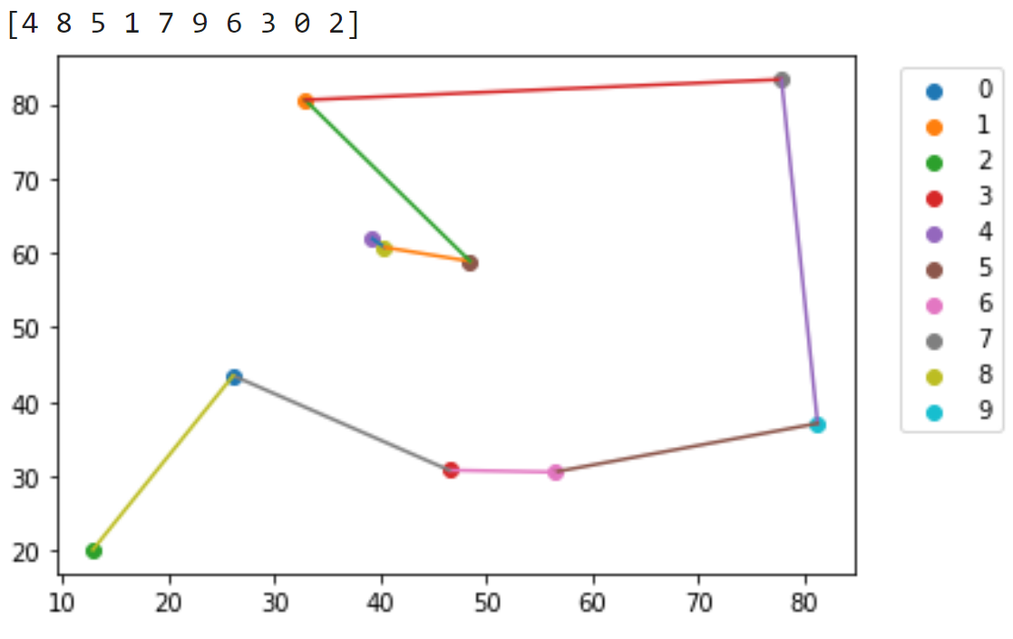
The figure shown below is a result generated with my approach. The path looks reasonably optimal. However, it is not the globally optimal solution. Furthermore, the model's solution converges to is highly dependent on how the model weights are initialized, which is randomly initialized.

I tried annealing techniques to address the optimal local issue, but it didn't fix the problem. Perhaps Markov Chain Monte Carlo methods might be better suited for optimizing such landscapes.

Additionally, I tested the method on problems with sizes ranging from 5-20 nodes. The solutions found did not have a consistent approximation ratio to that of the optimal solution. An in-depth analysis of the approach would be required to draw empirical bounds on the solutions of the method here. However, in theory, the technique can be applied to a problem of any size as long as it fits in memory. The memory cost is $O(n^2)$, where $n$ is the number of nodes in the problem.

However, one thing to consider is that the method, although not practical, is rather interesting. I found some papers that used Deep neural networks to solve the problem, but most of those used Graph neural networks and assumed a training dataset was available. The dataset is a set of arbitrary graphs and the optimal node visitation order as the labels. Such methods are black-box approaches; in contrast, mine is a closed-form formulation. Perhaps we can combine the two techniques to develop a superior method that can leverage the closed-form optimization metric along with the black box approaches excellent performance to reduce the amount of data that is required to train such models.

Formulation

The formulation starts with a randomly generated matrix $W$ of size $n \times n$. Here $n$ is the number of nodes in the TSP. The matrix values represent the probability of visiting each node at a particular step in the path. The columns are interpreted as the step-index of the generated path, and the rows are the node indices. So, the entry at row 2 and column 4 would correspond to the node probability of visiting node two at step 4 of the generated path.

The initial random matrix won't correspond to any valid path. Still, after optimization, the matrix will converge to a solution such that each column assigns a high probability to a single node that is supposed to be visited at a particular path step-index.

The optimization objective has two terms, a total path length and a constraint to enforce a continuous path. The constraint term is weighted with a scalar value.

$f = \text{Total Path Length} + (\text{Continuity Constraint} \times \lambda)$

First, we compute the total path length of the path selected by the path matrix $W$. Assuming that the path matrix is binary, one would calculate the total path length by summing the distance of each chosen edge. However, here the path matrix has a probabilistic interpretation, so we have to compute the total path length while considering the likelihood of each selected edge.

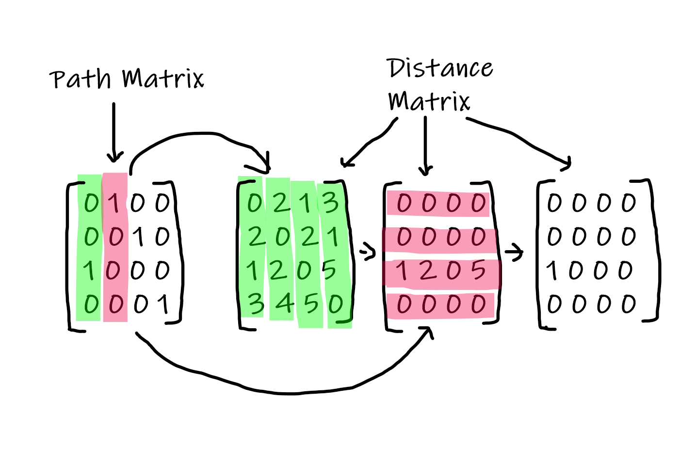
The path length is computed by composing the path matrix with the distance matrix. The distance matrix is a $n \times n$ matrix that contains the pairwise distances between the nodes. The distance matrix's rows can be interpreted as the start node and the column as the destination node. This interpretation allows us to apply the path matrix to the distance matrix with matrix operations.

We assume that the path matrix columns are binary, and each has a single node with a value of one and defines the matrix operations in two steps. First, we consider one column of the path matrix. This column represents the start node for an edge. Since the distance matrix's rows represent the start node, we multiply the column of the path matrix to each column of the distance matrix elementwise, the resulting distance matrix will have a single row with non-zero values, which is the row corresponding to the node selected by the path matrix column.

We now select the column next to the previously selected column in the path matrix and assume that it is the end node of the edge. And we multiply the column to the previously reduced distance matrix but now across the rows of the matrix. The resulting distance matrix would have a single non-zero entry at the start-end node pair given by the two adjacent columns of the path matrix.

This process of selecting adjacent columns and applying to the distance matrix is repeated for each edge of the path. The resulting distance matrices are summed up to get a single scalar path length. If the method is applied to a non-binary path matrix, the result can be interpreted as a probabilistic computation of the total path length. The following figure illustrates the process.

The optimized path matrix can select the same node in every column, which will result in a total path cost of 0. We can address this problem with an entropy constraint. By requiring each row of the path matrix to have high entropy, we can enforce a path constraint on the model. We want to avoid selecting the same node in multiple columns; requiring the entropy of each row to be high will make sure that the row has a single mode, thereby maximizing the entropy.

The path matrix is optimized jointly with the two optimization terms combined with a lagrangian term. I used the Adam optimizer to optimize the model.

import torch
import numpy as np
import torch.nn as nn
import matplotlib.pyplot as plt
from scipy.spatial.distance import pdist, squareform
from python_tsp.exact import solve_tsp_dynamic_programming

num_nodes = 10 # number of nodes in the TSP probelm
epochs = 1000 # number of epochs to train the model for
device = torch.device('cpu')

# Generate random point locations and compute pairwise distances
locs = np.random.rand(num_nodes, 2)*100
dist_mat = squareform(pdist(locs, 'euclidean'))
np.fill_diagonal(dist_mat, 1000.)
dist_mat = torch.from_numpy(dist_mat)

'''
Class to setup TSP problem as a continuous optimization problem
'''
class TSP(nn.Module):
    def __init__(self, num_nodes):
        super().__init__()
        self.num_nodes = num_nodes 
        # Weight matrix that is optimized to solve the problem
        self.weights = torch.nn.Parameter(torch.rand((num_nodes, num_nodes), 
                                                     dtype=torch.float64),
                                          requires_grad=True)
        self.softmax0 = nn.Softmax(dim=0)
        self.loss_lambda = torch.nn.Parameter(torch.tensor(0.5), 
                                              requires_grad=False)
               
    def forward(self, dist_mat):
        # compute softmax to concentrate predictions into point masses
        assign_mat = self.softmax0(self.weights)
        
        # apply softmax predicted path to distance matrix and compute total path length
        
        # create zero matrix to hold start node probabilities of each edge
        assign_mat_start = torch.zeros_like(assign_mat)
        # fill zero matrix with softmax predicted path node probabilities
        assign_mat_start[:, :-1] = assign_mat[:, :-1]
        # multiply node probabilites with distance matrix to select all start nodes
        node_ids = torch.unsqueeze(assign_mat_start, 0).T*dist_mat
        
        # create zero matrix to hold end node probabilities of each edge
        assign_mat_to = torch.zeros_like(assign_mat)
        # fill zero matrix with softmax predicted path node probabilities
        assign_mat_to[:, :-1] = assign_mat[:, 1:]
        # multiply node probabilites with previously computed start node filterted distance matrix
        node_ids = torch.unsqueeze(assign_mat_to, 1).T*node_ids     
        # sum reduced distance matrix to get total path length
        path_length = torch.sum(node_ids)
        
        # Add constrainet to make sure each node is selected only once in the path
        row_sums = torch.sum(assign_mat, dim=1)
        spread_cost = torch.sum(torch.abs(torch.ones(self.num_nodes)-row_sums))
        
        return self.loss_lambda*(200.*(spread_cost)) + path_length, assign_mat

    
# Create TSP model and use Adam optimized to optimize the model
model = TSP(num_nodes).to(device)
optimizer = torch.optim.Adam(model.parameters(), lr=1e-1) 
        
loss_plot = []
lamb = []
for epoch in range(epochs):      
    loss, predictions = model(dist_mat)
    optimizer.zero_grad()
    loss.backward()
    optimizer.step()
    loss_plot.append(loss.detach().cpu().numpy())
    model.loss_lambda.data = torch.tensor(0.5+0.01*np.sin(0.1*epoch))
    path = np.argmax(predictions.detach().cpu().numpy(), axis=0)
    
# Plot model loss
print("Model loss")
plt.plot(loss_plot)
plt.show()

# Plot predicted path matrix 
print("Model predicted path")
plt.imshow(predictions.detach().cpu().numpy())
plt.show()

# Plot predicted path
path = np.argmax(predictions.detach().cpu().numpy(), axis=0)
distance = 0
for i in range(len(path)-1):
    distance += dist_mat[path[i], path[i+1]]
    
print("Continuous formulation path and total distance")
print(list(path), distance.numpy())
for i, loc in enumerate(locs):
    plt.scatter(loc[0], loc[1], label=i)
plt.legend(bbox_to_anchor=(1.2, 1), loc='upper right')

for i in range(len(path)-1):
    plt.plot(locs[path[i:i+2], 0], locs[path[i:i+2], 1])
plt.show()
    
print("Dynamic Programmming formulation path and total distance")
path, distance = solve_tsp_dynamic_programming(dist_mat)
print(path, distance.numpy())
for i, loc in enumerate(locs):
    plt.scatter(loc[0], loc[1], label=i)
plt.legend(bbox_to_anchor=(1.2, 1), loc='upper right')

for i in range(len(path)-1):
    plt.plot(locs[path[i:i+2], 0], locs[path[i:i+2], 1])
plt.show()

Model loss

Model predicted path

Continuous formulation path and total distance
[0, 7, 3, 5, 2, 9, 8, 6, 1, 4] 304.5688834547842

Dynamic Programmming formulation path and total distance
[0, 4, 7, 1, 5, 3, 9, 8, 2, 6] 296.23342850439303

References:

http://iid.yale.edu/files/icml-2020/module3.pdf (Optimization landscape figure)

Libraries:

• Linear Algebra: https://numpy.org/
• Plotting: https://matplotlib.org/
• Backpropagation: https://pytorch.org/