---
title: "Generalized Linear Models"
author: "Kevin Donovan"
date: "`r format(Sys.time(), '%B %d, %Y')`"
output: slidy_presentation
---
```{r setup, include=FALSE}
knitr::opts_chunk$set(echo=FALSE, message = FALSE, warning = FALSE, fig.width = 8,
fig.height = 4)
library(tidyverse)
library(readr)
library(shiny)
library(rmarkdown)
library(dagitty)
library(ggdag)
library(broom)
library(flextable)
library(ggpubr)
library(nlme)
library(lme4)
library(mice)
library(naniar)
```
# Introduction
**Recall**: Discussed association analyses with correlation and linear regression
$$
\begin{align}
&Y=\beta_0+\beta_1X_1+\ldots+\beta_pX_p+\epsilon \\
&\\
&\text{where E}(\epsilon)=0 \text{; Var}(\epsilon)=\sigma^2 \\
&\epsilon_i \perp \epsilon_j \text{ for }i\neq j; X_1,\ldots,X_p\perp \epsilon
\end{align}
$$
- What about for discrete outcomes and non-normal error terms?
# Generalized linear model
- **Idea**: Create more general model structure to handle many distributions for outcome and residuals
- Keep flexibility and interpretability of linear regression model
- Especially flexibility with predictors/covariates (allow continuous, categorical, transformations, etc.)
- Such a structure referred to as *generalized linear models* or GLMs
- Focus on distribution of **outcome** instead of disribution of residuals
# Regression for binary outcomes
- Suppose we want to assess association between binary outcome and predictors
- Ex. Autism (ASD) diagnosis
- What if we use a linear regression model?
- $ASD=\beta_0+\beta_1X_1+\ldots+\beta_pX_p+\epsilon$
- $E(ASD|X)=\beta_0+\beta_1X_1+\ldots+\beta_pX_p$
- For binary $Y$, $\text{E}(Y|X)=\text{Pr}(Y=1|X)$
- $\rightarrow \text{Pr}(ASD=\text{Yes}|X)=\beta_0+\beta_1X_1+\ldots+\beta_pX_p$
- Denoted *linear probability model*
- **Limitation**: $0 \leq\text{Pr}(Y=1|X) \leq 1$ but linear function not constrained
# Logistic regression
- Specify transformation of probability which is **not constrained**, use linear model
- **Model**: Single Feature $X$
- $\text{logit}[p(ASD=\text{Yes}|X)]=\beta_0+\beta_1X$
- $\text{logit}(p)=\text{ln}(\frac{p}{1-p})=\text{log}( \text{odds}[p(Y=1|X)])$
- This, modeling **log odds** as a linear function of predictors **not probability**
- **In terms of conditional probability**:
- $p(ASD=\text{Yes}|X)=\frac{e^{\beta_0+\beta_1X}}{1+e^{\beta_0+\beta_1X}}$
- Can transform logit model to represent probabilities of interest
# Logistic regression
- Visualization between probability $p$ and $\text{logit}(p)$
```{r fig.width = 12, fig.height = 4}
logit <- function(x){
log(x/(1-x))
}
exbit <- function(x){
exp(x)/(1+exp(x))
}
x_domain_p <- seq(0, 1, by=0.01)
x_domain_p[x_domain_p==0] <- 0.01
x_domain_p[x_domain_p==1] <- 0.99
y_logit <- logit(x_domain_p)
x_domain_logit <- y_logit
y_exbit <- exbit(x_domain_logit)
plot_data <- data.frame(x_domain_p, y_logit, x_domain_logit, y_exbit)
prob_to_logit_plot <-
ggplot(data=plot_data,
mapping=aes(x=x_domain_p, y=y_logit))+
geom_line()+
xlab("Conditional Probability")+
ylab("Logit")+
labs(title = "Transforming probability to logit: logit(p)")+
theme_classic()+
theme(text = element_text(size=15))
logit_to_prob_plot <-
ggplot(data=plot_data,
mapping=aes(x=x_domain_logit, y=y_exbit))+
geom_line()+
xlab("Logit")+
ylab("Inverse Logit (Conditional Probability)")+
labs(title =
expression(paste("Transforming logit to probability: ",
frac(e^{x},1+e^{x}))))+
theme_classic()+
theme(text = element_text(size=15))
ggarrange(plotlist = list(prob_to_logit_plot, logit_to_prob_plot),
nrow=1)
```
# Logistic regression
- Visualization between probability $p$ and $\text{logit}(p)$ modeling ASD diagnosis
```{r fig.width = 12, fig.height = 4, echo=FALSE}
ibis_data <- read_csv(file = "../Data/Cross-sec_full.csv", na=c("",".","NA","N/A")) %>%
mutate(SSM_ASD_v24_num = ifelse(SSM_ASD_v24=="YES_ASD", 1,
ifelse(SSM_ASD_v24=="NO_ASD", 0, NA)))
ibis_data_nona <-
model.frame(lm(SSM_ASD_v24_num~`V24 mullen,composite_standard_score`,
data=ibis_data))
ibis_data_nona$prob_asd_linear <-
predict(lm(SSM_ASD_v24_num~`V24 mullen,composite_standard_score`,
data=ibis_data), newdata = ibis_data_nona)
ibis_data_nona$prob_asd_logit <-
predict(glm(SSM_ASD_v24_num~`V24 mullen,composite_standard_score`,
family=binomial(),
data=ibis_data), newdata = ibis_data_nona)
ibis_data_nona$prob_asd_logistic =
exp(ibis_data_nona$prob_asd_logit)/(1+exp(ibis_data_nona$prob_asd_logit))
scatter_linear <-
ggplot(data = ibis_data_nona,
mapping = aes(x=`V24 mullen,composite_standard_score`, y=SSM_ASD_v24_num))+
geom_point(aes(color=factor(SSM_ASD_v24_num)))+
geom_line(mapping=aes(y=prob_asd_linear))+
scale_y_continuous(breaks=seq(0, 1.2, 0.2))+
labs(x="24 Month MSEL Composite Score", y="ASD Diagnosis (1=YES)",
color="ASD Diagnosis")+
theme_classic()+
theme(legend.position = "none")
scatter_logistic <-
ggplot(data = ibis_data_nona,
mapping = aes(x=`V24 mullen,composite_standard_score`, y=SSM_ASD_v24_num))+
geom_point(aes(color=factor(SSM_ASD_v24_num)))+
geom_line(mapping=aes(y=prob_asd_logistic))+
scale_y_continuous(breaks=seq(0, 1.2, 0.2))+
labs(x="24 Month MSEL Composite Score", y="ASD Diagnosis (1=YES)",
color="ASD Diagnosis")+
theme_classic()+
theme(legend.position = "none")
ggarrange(plotlist=list(scatter_linear, scatter_logistic),
nrow = 1)
```
# Model fitting
- Since distribution of outcome based on covariates directly modeled, use *maximum likelihood* instead of least squares from before
# Maximum likelihood example
- **Intuition**:
- Find estimates of $\beta$ which best match with observed data, assuming data generated from **specified likelihood**
- Specifying the likelihood directly makes calculations more feasible, but assumptions **may not hold** (more on this later)
- Fitting in `R`: `glm` function
```{r, echo=FALSE}
glm_fit <-
glm(factor(SSM_ASD_v24)~`V24 mullen,composite_standard_score`,
family=binomial(),
data=ibis_data)
# Raw output
summary(glm_fit)
# Format output
tidy(glm_fit) %>%
mutate(p.value=ifelse(p.value<0.005, "<0.005",
as.character(round(p.value, 3))),
term=fct_recode(factor(term),
"Intercept"="(Intercept)",
"24 Month MSEL Composite Standard Score"=
"`V24 mullen,composite_standard_score`")) %>%
flextable() %>%
set_header_labels("term"="Variable",
"estimate"="Estimate",
"std.error"="Std. Error",
"statistic"="Z Statistic",
"p.value"="P-value") %>%
autofit()
```
# Logistic regression
**Estimated model**:
$\hat{\text{Pr}}[ASD=\text{YES}|MSEL]=\frac{e^{6.67-0.09MSEL}}{1+e^{6.67-0.09MSEL}}$
**Interpretation**:
1. $\hat{\beta_0}=6.67$
- $\hat{\text{Pr}}[ASD=\text{YES}|MSEL=0]=\frac{e^{6.67}}{1+e^{6.67}}$
2. $\hat{\beta_1}=-0.09$
- $\rightarrow$ Probability of ASD diangosis **decreases** as MSEL **increases**
# Logistic regression
**Intercept**:
- MSEL = 0 doesn't make sense
**Solution**: center at means
- MSEL - $\mu$ = 0 $\rightarrow$ MSEL = $\mu$
```{r}
ibis_data <- ibis_data %>%
mutate(mullen_center = `V24 mullen,composite_standard_score` -
mean(`V24 mullen,composite_standard_score`, na.rm=TRUE))
glm_fit <-
glm(factor(SSM_ASD_v24)~mullen_center,
family=binomial(),
data=ibis_data)
# Raw output
summary(glm_fit)
# Format output
tidy(glm_fit) %>%
mutate(p.value=ifelse(p.value<0.005, "<0.005",
as.character(round(p.value, 3))),
term=fct_recode(factor(term),
"Intercept"="(Intercept)",
"24 Month MSEL Composite Centered"=
"mullen_center")) %>%
flextable() %>%
set_header_labels("term"="Variable",
"estimate"="Estimate",
"std.error"="Std. Error",
"statistic"="Z Statistic",
"p.value"="P-value") %>%
autofit()
```
**Interpretation**:
1. $\hat{\beta_0} = -2.34$
$$
\hat{\text{Pr}}[ASD=\text{YES}|MSEL=\mu]=\frac{e^{-2.34}}{1+e^{-2.34}}
$$
Slope $\hat{\beta_1}$ not changed
# Logistic Regression
Model-based estimated probabilities (non-centered):
For patient with MSEL=100 (mean in population for standard score)
$$
\hat{\text{Pr}}[ASD=\text{YES}|MSEL=90]=\frac{e^{6.67-0.09*90}}{1+e^{6.67-0.09*90}}=0.19
$$
Based on $\hat{\text{Pr}}[ASD=\text{YES}|MSEL=90]$ can create predicted response $\hat{ASD}$ by thresholding
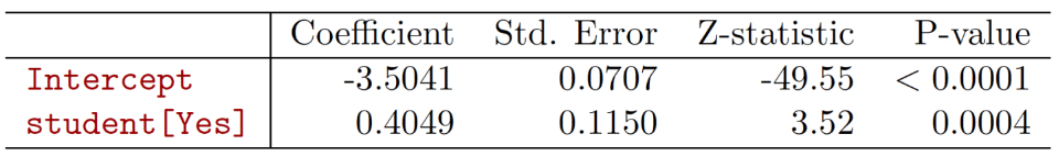
# Logistic regression: confounding
**Example**: Credit Card Default Rate
- Consider predicting if a person defaults on their loan based on
- Student Status (Student or Not Student):
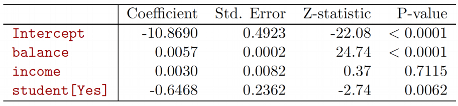
- Now consider adding features: `credit balance` and `income`
- Why did `student`'s coefficient change so much? **Confounding**
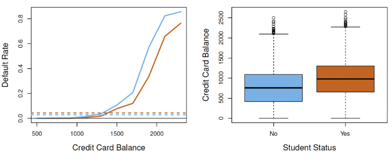
# Logistic regression: confounding
- Being a student $\rightarrow$ higher balance (more loans)
- $\rightarrow$ higher marginal default rate vs non-students
- But is it the higher balance or simply them being students leading to defaulting more often?
- Need to compare students and non-students **controlling** for balance to answer this
- Can be done using regression
# Generalized linear models
- Logistic regression one example of a GLM
**Structure of model**:
1. Choose conditional distribution $f(y|x)$
- Linear regression: $f(y|x)\sim \text{Normal}(\mu_{y|x}, \sigma^2)$
- $\mu_{y|x} = \text{E}(Y|X); \sigma^2=\text{Var}(Y|X)=\text{Var}(\epsilon)$
- Logistic regression: $f(y|x)\sim \text{Binomial}[p(x)]$
- $p(x) = \mu_{y|x} = \text{Pr}(Y=1|X)$
# Generalized linear models
2. Choose *link function* $g(\mu_{y|x})=\beta_0+\beta_1X_1+\ldots+\beta_pX_p$
- Linear regression: $g(\mu_{y|x})=\mu_{y|x}$
- Logistic regression $g(\mu_{y|x})=\log(\frac{\mu_{y|x}}{1-\mu_{y|x}})$
- **Idea**: $g(\mu_{y|x}):\mathcal{X}_\mu \rightarrow (-\infty, \infty)$
3. Construct likelihood and fit
- Assuming independent observations:
- $f(y|x)=\prod_{i=1}^{n} f(y_i|x_i)$
# Generalized linear models
- Examples include
- Poisson regression (outcome is a count)
- Gamma regression (outcome is skewed and non-negative)
- Multinomial logistic (categorical outcome, 2+ categories)
- Beta, negative binomial, etc.
- Most can be fit all using the `glm`() function in R
- some, like beta, negative binomial, *overdispered* Poisson, etc. require other packages