**What data to use for what process?**
Need sufficient sample to learn patterns
Train and test on same data $\rightarrow$ **bias**
What do we mean by *bias*?
# Bias, generalizability, variance
:::: {style="display: flex;"}
::: {}
- Generalizability
- Algorithm performs well on **independent samples** from population
- Higher level: generalizes to **different populations**
- Bias
- **Average over/underperformance** in independent sample vs. observed sample
- **Only see performance in observed sample**, biased results can be very dangerous!
- Variance
- Algorithm's accuracy and results differ based on examined data
- **Not good!** Limits certainty in observed results
:::
::: {}
:::
::::
# Loss function
:::: {style="display: flex;"}
::: {}
- Need some measure of an algorithm's "accuracy/error" for it to learn
- Metric used called *loss function*
- Varies depending on method or model used
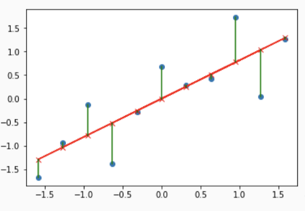
- Ex. residual sum of squares
$$
\begin{align}
&Y_i = \text{outcome for person }i \\
&X_i = \text{predictor value for person }i \\
&\text{Model: }\hat{Y}_i=\beta_0+\beta_1X_i \\
& \\
&\text{Loss function: }L(\beta_0, \beta_1,Y,X)=\sum_{i=1}^{n}[Y_i-(\beta_0+\beta_1X_i)]^2\\
&\{\hat{\beta}_0, \hat{\beta}_1\} = \{\beta_0, \beta_1\} \text{ which minimizes } L(\beta_0, \beta_1,Y,X)
\end{align}
$$
:::
::: {}
:::
::::
# Supervised learning
- Learning when outcome of interest is **observed**
- Common example: predicting observed trait (diagnosis)
- Can use observed trait in training data to *learn patterns* with predictor variables
- Predictor variables often called *features*
- Differs with *unsupervised learning* (trait **not observed**)
:::: {style="display: flex;"}
::: {}
:::
::: {}
:::
::::
# Models and tuning
:::: {style="display: flex;"}
::: {}
- Various models used to train supervised learning algorithm
- Examples
1. Linear regression
2. Logistic regression
3. Penalized regression
4. K-means
5. Decision trees
6. Support vector machines
7. Neural networks (*deep learning*)
- Each has set of *tuning parameters* which alter their specific structure
- Ex. K-means: $k$ = # of neighbors in a neighborhood
- After tuning set, then model is fixed and training can be done
- How to determine tuning parameters?
:::
::: {}
:::
::::
# Testing
:::: {style="display: flex;"}
::: {}
- Unbiased testing $\rightarrow$ independent dataset needed
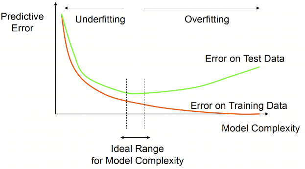
- Training results may *overfit to training data* $\rightarrow$ **not** reliable metric for general performance
- Where to get independent dataset?
- Testing data sources:
1. Completely separate sample (from same or different population)
2. Random partition into 2/3 parts
3. Random partition into $k$ parts, repeat training and testing process
- Called *k-fold cross validation* (k-fold CV)
:::
::: {}
:::
::::
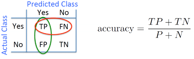
# Testing
- Metrics
- Must choose metrics to quantify algorithm's accuracy/utility
- Choice depends on many factors:
1. Continuous or categorical outcome?
2. Should certain values be weighted differently? (cost may vary by outcome)
3. What is the purpose of the algorithm (ex. screening tool)?
:::: {style="display: flex;"}
::: {}
:::
::: {}
:::
::::
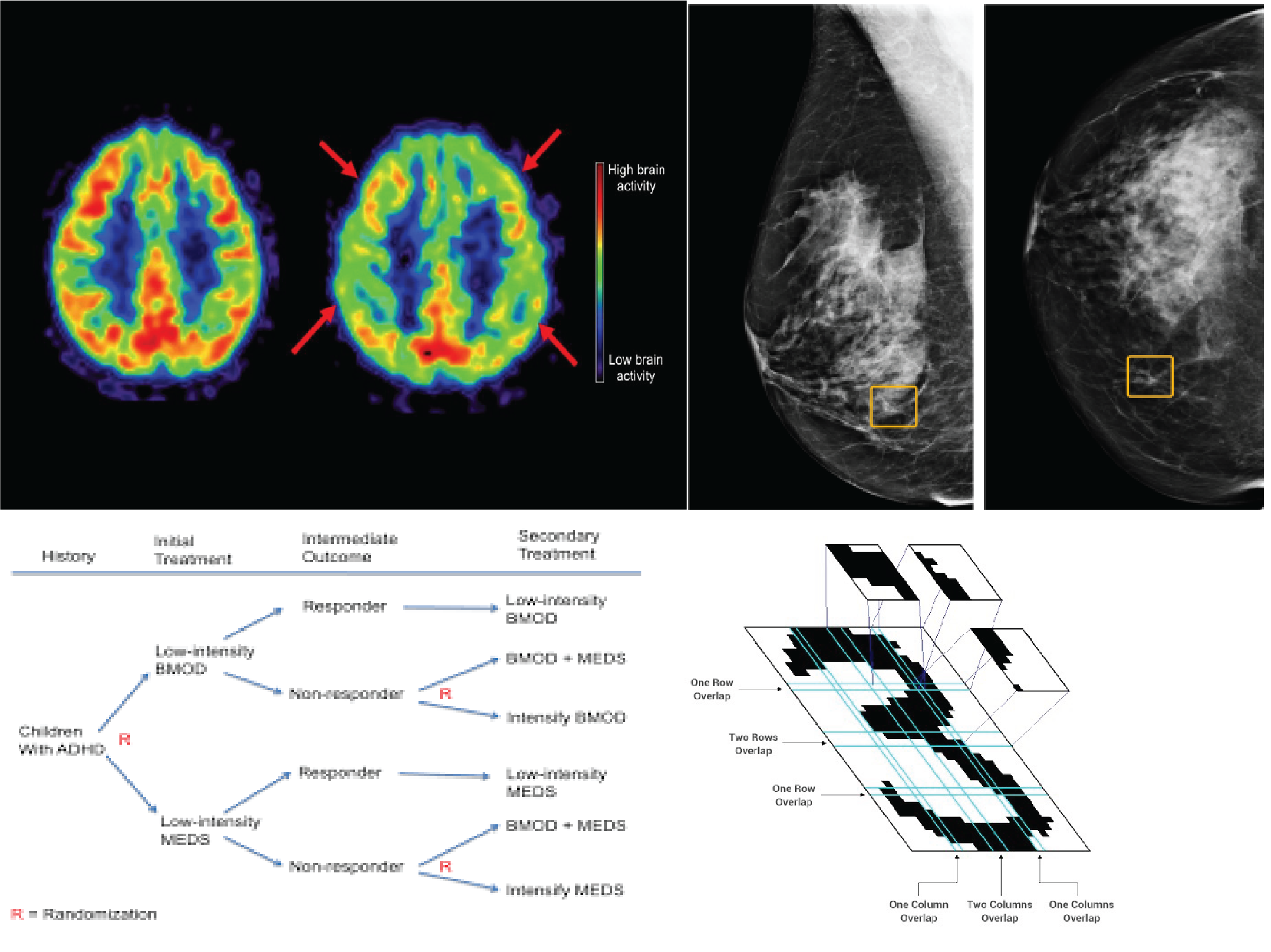
# Examples in research
# Example with IBIS
- Let's go through examples using IBIS data
- Will go step-by-step
- Discuss additional complications that may arise
- Discuss potential areas of bias and inefficiency
- Illustrate various methods
# Predicting ASD Diagnosis
- In all cases, we will be attempting to **predict 24 month Autism (ASD) diagnosis**
- Will try using brain and behavioral measures at 12 months
- Starting point: simple brain model
- Total brain volume and EACSF at 12 months
```{r}
ggplot(data=ibis_brain_data, mapping=aes(x=EACSF_V12, y=TBV_V12, color=RiskGroup))+
geom_point()+
theme_bw()
```
# Predicting ASD Diagnosis
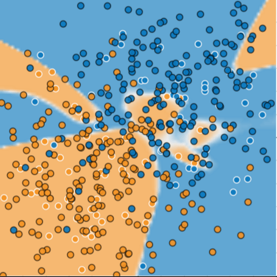
- **Step 1**: Select model
- We consider K-Nearest Neighbor (KNN) and logistic regression
- KNN visualized below
```{r fig.width = 5, fig.height = 5}
# KNN fitting on whole data
ibis_brain_data_complete <-
ibis_brain_data %>%
drop_na() %>%
mutate(RiskGroup = factor(RiskGroup)) %>%
data.frame()
ibis_brain_data_complete_smote <- SMOTE(RiskGroup~EACSF_V12+TBV_V12,
data = ibis_brain_data_complete,
perc.under = 150)
# Code to plot neighborhoods
decisionplot <- function(model, data, class = NULL, predict_type = "class",
resolution = 100, showgrid = TRUE, ...) {
if(!is.null(class)) cl <- data[,class] else cl <- 1
data <- data[,colnames(model$learn$X)]
k <- length(unique(cl))
plot(data, col = as.integer(cl)+1L, pch = as.integer(cl)+1L, ...)
# make grid
r <- sapply(data, range, na.rm = TRUE)
xs <- seq(r[1,1], r[2,1], length.out = resolution)
ys <- seq(r[1,2], r[2,2], length.out = resolution)
g <- cbind(rep(xs, each=resolution), rep(ys, time = resolution))
colnames(g) <- colnames(r)
g <- as.data.frame(g)
### guess how to get class labels from predict
### (unfortunately not very consistent between models)
p <- predict(model, g, type = predict_type)
if(is.list(p)) p <- p$class
p <- as.factor(p)
if(showgrid) points(g, col = as.integer(p)+1L, pch = ".")
z <- matrix(as.integer(p), nrow = resolution, byrow = TRUE)
contour(xs, ys, z, add = TRUE, drawlabels = FALSE,
lwd = 2, levels = (1:(k-1))+.5)
invisible(z)
}
knn_all_data_fit <-
knn3(RiskGroup~EACSF_V12+TBV_V12, data=ibis_brain_data_complete_smote, k=5)
decisionplot(model=knn_all_data_fit, data=ibis_brain_data_complete_smote,
class = "RiskGroup", main = "kNN (5)")
knn_all_data_fit <-
knn3(RiskGroup~EACSF_V12+TBV_V12, data=ibis_brain_data_complete_smote, k=30)
decisionplot(model=knn_all_data_fit, data=ibis_brain_data_complete_smote,
class = "RiskGroup", main = "kNN (30)")
```
# Predicting ASD Diagnosis
- **Step 2**: Select training and testing set strategy
- Generally, will need to use *holdout* method (often hungry for more data!)
- Single train-test split or CV? If CV how many folds?
- Considerations
- Interpretability
- Bias-variance trade-off
```{r fig.width = 7, fig.height = 4}
## Set degrees being considered:
wage_data <- Wage # contained in ISLR package
degrees <- 1:10
poly_reg_fit <- list()
error_rates_degrees <- list()
# Fit model for each degree considered, compute RMSE (on training in this ex.)
for(i in 1:length(degrees)){
poly_reg_fit[[i]] <- lm(wage~poly(age, degrees[i]),
data=wage_data)
predict_wages <- predict(poly_reg_fit[[i]])
residuals_wages <- wage_data$wage-predict_wages
rmse_poly_reg <- sqrt(mean(residuals_wages^2))
mae_poly_reg <- mean(abs(residuals_wages))
# Save in data frame
error_rates_degrees[[i]] <-
data.frame("RMSE"=rmse_poly_reg,
"MAE"=mae_poly_reg,
"degree"=degrees[i])
}
# Bind all degree-specific results together into single data frame/table
error_rates_degrees_df <- do.call("rbind", error_rates_degrees)
# Plot results as function of degree
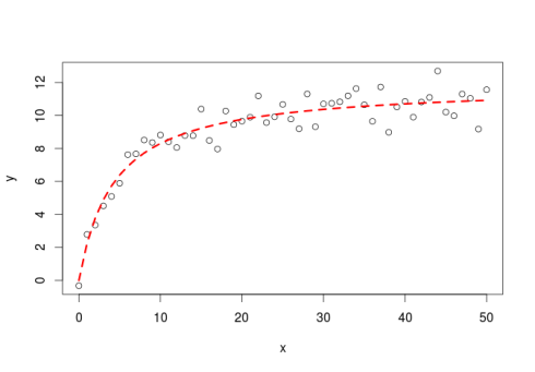
ggplot(data=error_rates_degrees_df,
mapping=aes(x=degrees, y=RMSE))+
geom_point()+
geom_line()+
labs(title="RMSE (Root Mean Squared Error) by degree without data splitting")
# Line continuously decreases, though seems improvement after 3 or 4 is minimal
# For better assessment, split into training (60:40 split for ex)
# Fit model for each degree considered, compute RMSE (on training in this ex.)
poly_reg_fit <- list()
error_rates_degrees <- list()
counter <- 1
trials <- 15 # Look at 15 different 60:40 splits
wage_data_subset <- wage_data[sample(1:dim(wage_data)[1], size=400, replace=FALSE),]
for(j in 1:trials){
set.seed(2*j) # Set seed to get different splits
tt_indicies <- createDataPartition(y=wage_data_subset$wage, p=0.6, list = FALSE)
wage_data_train <- wage_data_subset[tt_indicies,]
wage_data_test <- wage_data_subset[-tt_indicies,]
for(i in 1:length(degrees)){
poly_reg_fit[[counter]] <- lm(wage~poly(age, degrees[i]),
data=wage_data_train)
predict_wages <- predict(poly_reg_fit[[counter]], newdata = wage_data_test)
residuals_wages <- wage_data_test$wage-predict_wages
rmse_poly_reg <- sqrt(mean(residuals_wages^2))
mae_poly_reg <- mean(abs(residuals_wages))
# Save in data frame
error_rates_degrees[[counter]] <-
data.frame("RMSE"=rmse_poly_reg,
"MAE"=mae_poly_reg,
"degree"=degrees[i],
"split_trial"=j)
counter <- counter+1
}
}
# Bind all degree-specific results together into single data frame/table
error_rates_degrees_df <- do.call("rbind", error_rates_degrees)
# Plot results as function of degree
ggplot(data=error_rates_degrees_df,
mapping=aes(x=degree, y=RMSE, color=factor(split_trial)))+
geom_point()+
geom_line()+
labs(title="RMSE (Root Mean Squared Error) by degree on test set\nBy split number")+
theme_bw()
```
# Drawbacks of holdout
- Test set error can be highly dependent on split
- Thus **highly variable**
- Especially for small dataset or **small group sizes**
- Only subset of data used to train algorithm
- May result in poorer algorithm
- $\rightarrow$ may **overestimate** test error
- Can we **aggregate results over multiple test sets?**
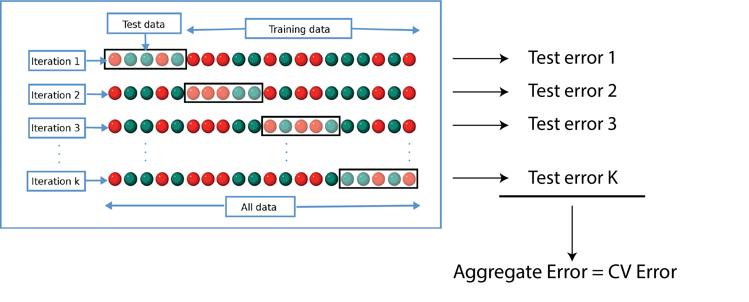
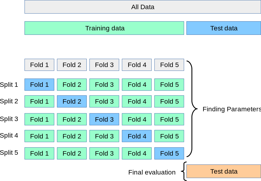
# K-fold cross validation
- Denote $K$ folds by $C_1, C_2, \ldots, C_K$, each with $n_k$ observations
- For a given fold $l$:
1. Train algorithm on data in other folds: $\{C_k\}$ s.t. $k\neq l$
2. Test by computing predicted values for data in $C_l$ **only**
3. Repeat for each fold $l=1, \ldots, K$, average error (ex. $MSE_l$)
- K fold CV error rate
$$
CV_{(K)}=\sum_{k=1}^{K}\frac{n_k}{n}MSE_k
$$
where $MSE_k=\sum_{i\in C_k}(y_i-\hat{y_i})^2/n_k$ where $y_i$ is outcome and $\hat{y_i}$ is predicted outcome from training on $C_k$ **only**
- $K=n$ yields $n-fold$ or *leave-one out cross-validation*
- $CV_{(K)}$ is accurate measure of generalized error rate for algorithm trained on whole sample
# CV for classification
- Same process as before, divide data into $K$ partitions $C_1, \ldots, C_K$
- Choose error/accuracy rate of interest
- E.g. sensitivity, specificity, classification error, etc.
- For classification error
- Compute CV error
$$
CV_K=\sum_{k=1}^{K}\frac{n_k}{n}\text{Error}_k=\frac{1}{K}\sum_{k=1}^{K}\text{Error}_k
$$
where $\text{Error}_k=\sum_{i \in C_k}I(y_i \neq \hat{y_i})/n_k$
- Can we estimate the **variability** of this estimate?
- Commonly used estimate of standard error:
$$
\hat{\text{SE}}(\text{CV}_K)=\sqrt{\sum_{k=1}^{K}(\text{Error}_k-\overline{\text{Error}_k})^2/(K-1)}
$$
- While useful, not accurate (**Why?**)
- Also can be used in continuous prediction CV (using MSE for example)
# CV visually
- Smoothed estimate of generalized error
# Choosing K: bias-variance tradeoff
- **Recall**: Holdout method uses only portion of data for training
- $\rightarrow$ test/validation performance **overestimate**
- $\rightarrow$ more folds $\rightarrow$ more data in training folds $\rightarrow$ better algorithm $\rightarrow$ lower mean error
- $\rightarrow$ LOOCV least biased estimate of test error
- Compared to hold out, each training set in K-fold contains $\frac{(k-1)n}{k}$ obs
- Generally more then in holdout $\rightarrow$ less biased estimate
# CV with tuning
- **Recall**: Often when training a prediction algorithm, need to select **tuning parameters**
- Ex. \# of neighbors with KNN
- Where is tuning implemented in CV?
- Example: Consider set of 5000 predictors and 50 samples of data
- 1. Starting with the 5000 predictors and full data, **first** find 100 predictors with largest correlation with outcome
- 2. Then train and test an algorithm with only these 100 predictors, using logistic regression as an example
- How do we estimate the algorithm's test set performance without bias?
- Can we only apply CV in step 2, after the predictors have been chosen using the full data?
# NO
- Why?
- This selection of parameters greatly impacts the algorithm's performance and thus is a form of tuning
- Tuning needs to be done within the training framework, otherwise you are training and testing on the same dataset
- Thus, need to do step 1 within your CV scheme
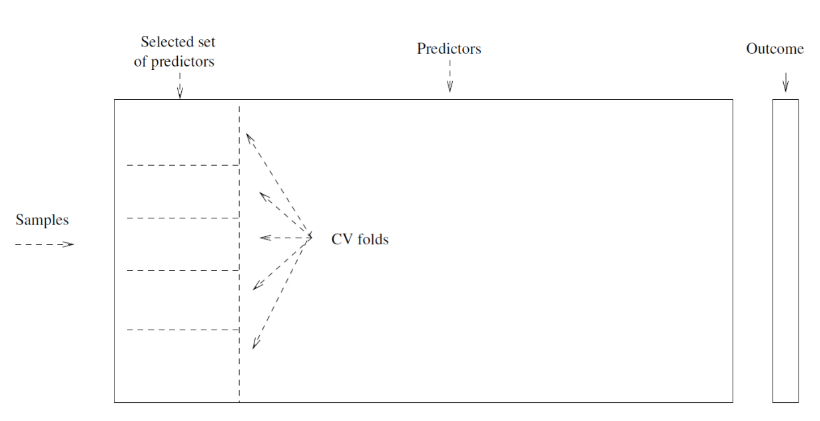
# Wrong way: visual
- Only doing step 2 inside CV process
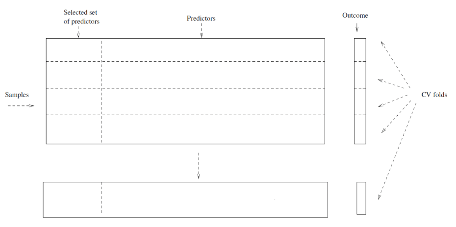
# Right way: visual
- Doing both steps 1 and 2 within CV process
# Right way: visual
- Make sure tuning and testing are done **on separate datasets!**
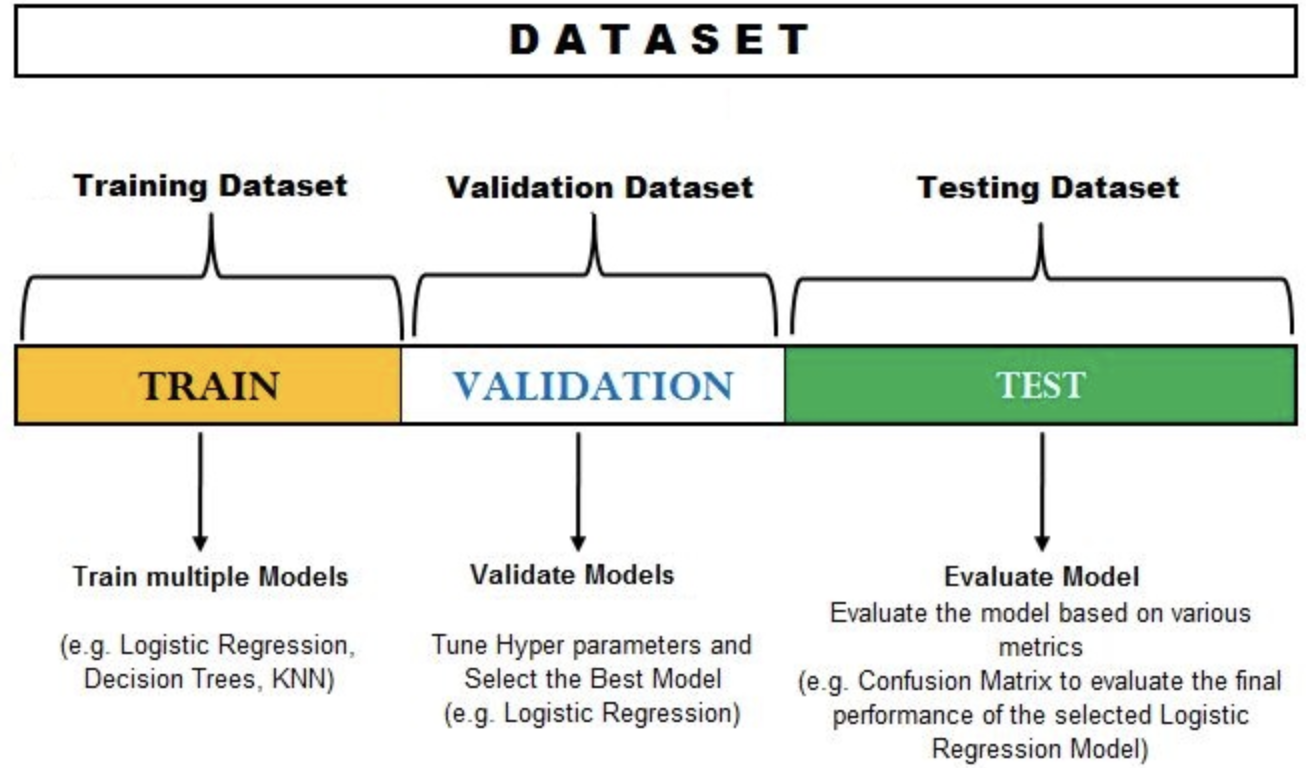
# Concept of a validation set
- Sometimes, **three** data paritions are created
- One for training, one for *validation*, and one for testing
- Validation dataset is specifically used for tuning
- Final fitting done on training+validation, evaluated on testing
- Separate training and tuning sets **may** $\rightarrow$ more generalizable tuning parameters selected
- Alternative: do CV with single training/tuning set when tuning (*nested* CV)
# Predicting ASD Diagnosis
- **Step 2**: Select training and testing set strategy
- Let's use KNN, tune within CV process using *nested* CV
- **Step 3**: Select metric
- Evaluate on test folds in CV process, CV sensitivity, specificity, etc.
- Other metrics also available, these suffice for two-group case
- Implementation in R: `train` and `createFolds` from `caret` package
- `train` can be used to tune and train many types of models
- `postResample` and `confusionMatrix` to see metrics
```{r echo=FALSE}
ibis_brain_data_complete <-
ibis_brain_data %>%
drop_na() %>%
mutate(RiskGroup = factor(RiskGroup)) %>%
data.frame()
```
```{r echo=TRUE, eval=FALSE}
knn_fit <-
train(RiskGroup~EACSF_V12+TBV_V12, data=ibis_brain_data_complete,
tuneLength=10, method="knn", preProcess = c("scale", "center")
trControl=trainControl(method="cv"))
```
# Implement in R: KNN
```{r echo=TRUE, eval=FALSE}
# Create folds
tt_indices <- createFolds(y=ibis_brain_data_complete$RiskGroup, k=10)
# Do train and test for each fold
for(i in 1:length(tt_indices)){
# Create train and test sets
train_data <- ibis_brain_data_complete[-tt_indices[[i]],]
test_data <- ibis_brain_data_complete[-tt_indices[[i]],]
knn_fit <-
train(RiskGroup~EACSF_V12+TBV_V12, data=train_data,
tuneLength=10, method="knn", preProcess = c("scale", "center")
trControl=trainControl(method="cv"))
}
```
# Implement in R: KNN
```{r echo=TRUE}
# Create folds
tt_indices <- createFolds(y=ibis_brain_data_complete$RiskGroup, k=10)
# Do train and test for each fold
cv_results <- list()
for(i in 1:length(tt_indices)){
# Create train and test sets
train_data <- ibis_brain_data_complete[-tt_indices[[i]],]
test_data <- ibis_brain_data_complete[-tt_indices[[i]],]
knn_fit <-
train(RiskGroup~EACSF_V12+TBV_V12, data=train_data,
tuneLength=10, method="knn", preProcess = c("scale", "center"),
trControl=trainControl(method="cv"))
# Save confusion matrix for each fold
cv_results[[i]] <- confusionMatrix(data=predict(knn_fit, newdata=test_data),
reference=test_data$RiskGroup,
positive="HR-ASD")
}
# Print confusion matrix for a fold
cv_results[[1]]
```
# Unbalanced Data
- Algorithm does terribly for ASD prediction but accuracy is high
- Good accuracy but poor sensitivity
- KNN (and most others) use general error as "loss function"
- $\rightarrow$ if minority class is very small, see **poor performance**
- Solutions
- Weighting: *weight* minority class more in error calculation
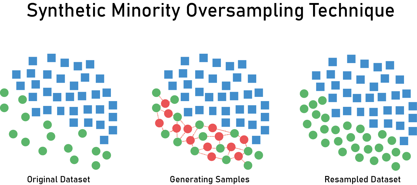
- Resampling: generate *synthetic sample* with balance between classes
- Ex. SMOTE
- Complications?
# Weighting
- By default, each obs gets same weight $\rightarrow$ contribute to error the same amount
- But, **error in predicting one type may have higher cost then for other type**
- Can implement this using chosen weights
- Ex. linear regression
- No weights
$$
\hat{y} = \underset{\beta}{\mathrm{argmin}}\sum_{i=1}^n(y_i-\beta x_i)^2
$$
- Weights
$$
\begin{align}
& \hat{y}_w = \underset{\beta}{\mathrm{argmin}}\sum_{i=1}^nw_i(y_i-\beta x_i)^2 \\
& \text{where } \{w_i\}_{i=1}^n \text{ are subject-specific weights}
\end{align}
$$
- Common choice for weights: *inverse probability weighting*
$$
\begin{align}
& w_i = 1/\hat{\pi}_k \text{ for } k=1,\ldots, K \\
& \text{where } \hat{\pi}_k=\sum_{i=1}^{n} I(i \text{ in group } K)/n
\end{align}
$$
- Those in rare groups get **high weight**, cost for their error is high
# Resampling
- Caveats:
- SMOTE requires **some** numeric predictors to determine ''neighborhoods'' to draw samples
- **Ad hoc**: convert categorical to numeric
- May be suboptimal (**Why?**)
- Can be difficult to select ROC-based threshold from training set after SMOTE
- Sometimes threshold chosen from test set, **but this is suboptimal!**
# Implement in R
- With `caret` can implement in `train` function (`weights` argument)
- Common SMOTE method: `DmWR` package
- **However**, package has been removed from CRAN
- Alternatives: `smotefamily` and `bimba`
# Examples
**Inverse probability weighting**
```{r echo=TRUE, eval=FALSE}
# Create training set weights per person
train_weights <- ifelse(ibis_brain_data_complete$RiskGroup=="HR-ASD",
1/prop.table(table(ibis_brain_data_complete$RiskGroup))["HR-ASD"],
1/prop.table(table(ibis_brain_data_complete$RiskGroup))["HR-Neg"])
knn_fit <-
train(RiskGroup~EACSF_V12+TBV_V12, data=ibis_brain_data_complete,
tuneLength=10, method="knn", preProcess = c("scale", "center")
trControl=trainControl(method="cv"))
```
**SMOTE**
```{r echo=TRUE}
# Look at frequencies
table(ibis_brain_data_complete$RiskGroup)
# Run SMOTE
ibis_brain_data_complete_smote <- SMOTE(RiskGroup~EACSF_V12+TBV_V12,
data = ibis_brain_data_complete,
perc.under = 150)
# Now look at frequencies
table(ibis_brain_data_complete_smote$RiskGroup)
knn_fit <-
train(RiskGroup~EACSF_V12+TBV_V12, data=ibis_brain_data_complete_smote,
tuneLength=10, method="knn", preProcess = c("scale", "center"),
trControl=trainControl(method="cv"))
```
# Logistic regression
- KNN can be adapted to compute probabilities of being in a class (see `knnflex`)
- Logistic regression models these probabilities directly
- Let's try this method instead
```{r echo=TRUE, eval=FALSE}
# Create folds
tt_indices <- createFolds(y=ibis_brain_data_complete$RiskGroup, k=10)
# Do train and test for each fold
cv_results <- list()
for(i in 1:length(tt_indices)){
# Create train and test sets
train_data <- ibis_brain_data_complete[-tt_indices[[i]],]
test_data <- ibis_brain_data_complete[-tt_indices[[i]],]
# Run logistic regression model
logreg_fit <-
glm(RiskGroup~EACSF_V12+TBV_V12, data=train_data,
family=binomial)
# Save confusion matrix for each fold, use 50% probability threshold
test_preds <- factor(ifelse(predict(logreg_fit, newdata=test_data, type="response")>0.5,
"HR-Neg", "HR-ASD"))
cv_results[[i]] <- confusionMatrix(data=predict(logreg_fit, newdata=test_data, type="response"),
reference=test_data$RiskGroup,
positive="HR-ASD")
}
cv_results[[1]]
```
# ROC Curve
- We chose a 0.5 threshold, but this may be suboptimal
- Why?
- Instead, can evaluate the performance at **all possible thresholds**
- Results in a set values which can be plotted: *ROC curve*
- Can summarize curve: area under the curve (AUC)
- Done in R using `pROC` and `ggroc`
```{r echo=TRUE}
# Run logistic regression model
logreg_fit <-
glm(RiskGroup~EACSF_V12+TBV_V12, data=ibis_brain_data_complete,
family=binomial)
# Get estimated probabilities of HR-ASD
est_probs <- 1-predict(logreg_fit, newdata=ibis_brain_data_complete, type="response")
# Compute ROC curve with AUC
roc_curve <- roc(response=ibis_brain_data_complete$RiskGroup,
predictor=est_probs,
levels=c("HR-Neg", "HR-ASD"))
# Plot ROC curve
ggroc(roc_curve)+
labs(title = paste0("AUC = ", round(auc(roc_curve),2)))+
theme_bw()
```
# ROC Curve
- Can use `ggroc` to customize plot more
- Can use various metrics to determine "best" threshold
- Ex. maximum Youden's index
```{r echo=TRUE}
# Return max Youden's index, with specificity and sensitivity
best_thres_data <-
data.frame(coords(roc_curve, x="best", best.method = c("youden", "closest.topleft")))
# View performance at "best threshold"
best_thres_data
data_add_line <-
data.frame("sensitvity"=c(1-best_thres_data$specificity,
best_thres_data$sensitivity),
"specificity"=c(best_thres_data$specificity,
best_thres_data$specificity))
ggroc(roc_curve)+
geom_point(
data = best_thres_data,
mapping = aes(x=specificity, y=sensitivity), size=2, color="red")+
geom_point(mapping=aes(x=best_thres_data$specificity,
y=1-best_thres_data$specificity),
size=2, color="red")+
geom_segment(aes(x = 1, xend = 0, y = 0, yend = 1),
color="darkgrey", linetype="dashed")+
geom_text(data = best_thres_data,
mapping=aes(x=specificity, y=0.90,
label=paste0("Threshold = ", round(threshold,2),
"\nSensitivity = ", round(sensitivity,2),
"\nSpecificity = ", round(specificity,2),
"\nAUC = ", round(auc(roc_curve),2))))+
geom_line(data=data_add_line,
mapping=aes(x=specificity, y=sensitvity),
linetype="dashed")+
theme_classic()
```