Basic histogram with geom_histogram
It is relatively straightforward to build a histogram with ggplot2 thanks to the geom_histogram() function. Only one numeric variable is needed in the input. Note that a warning message is triggered with this code: we need to take care of the bin width as explained in the next section.
# library
library(ggplot2)

# dataset:
data=data.frame(value=rnorm(100))

# basic histogram
p <- ggplot(data, aes(x=value)) +
  geom_histogram()

#p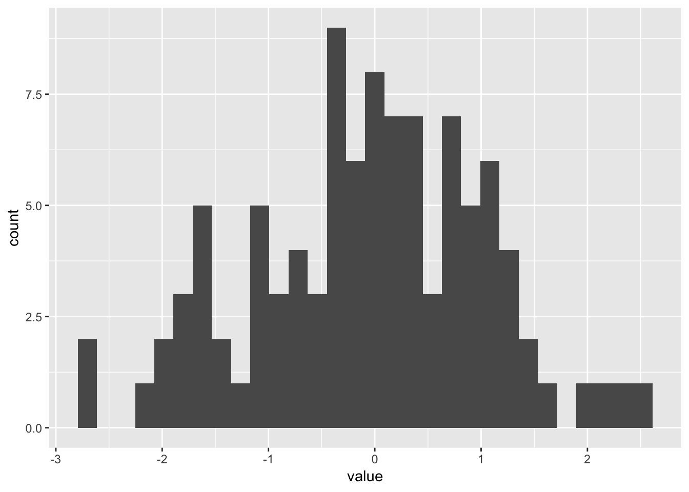
Control bin size with binwidth
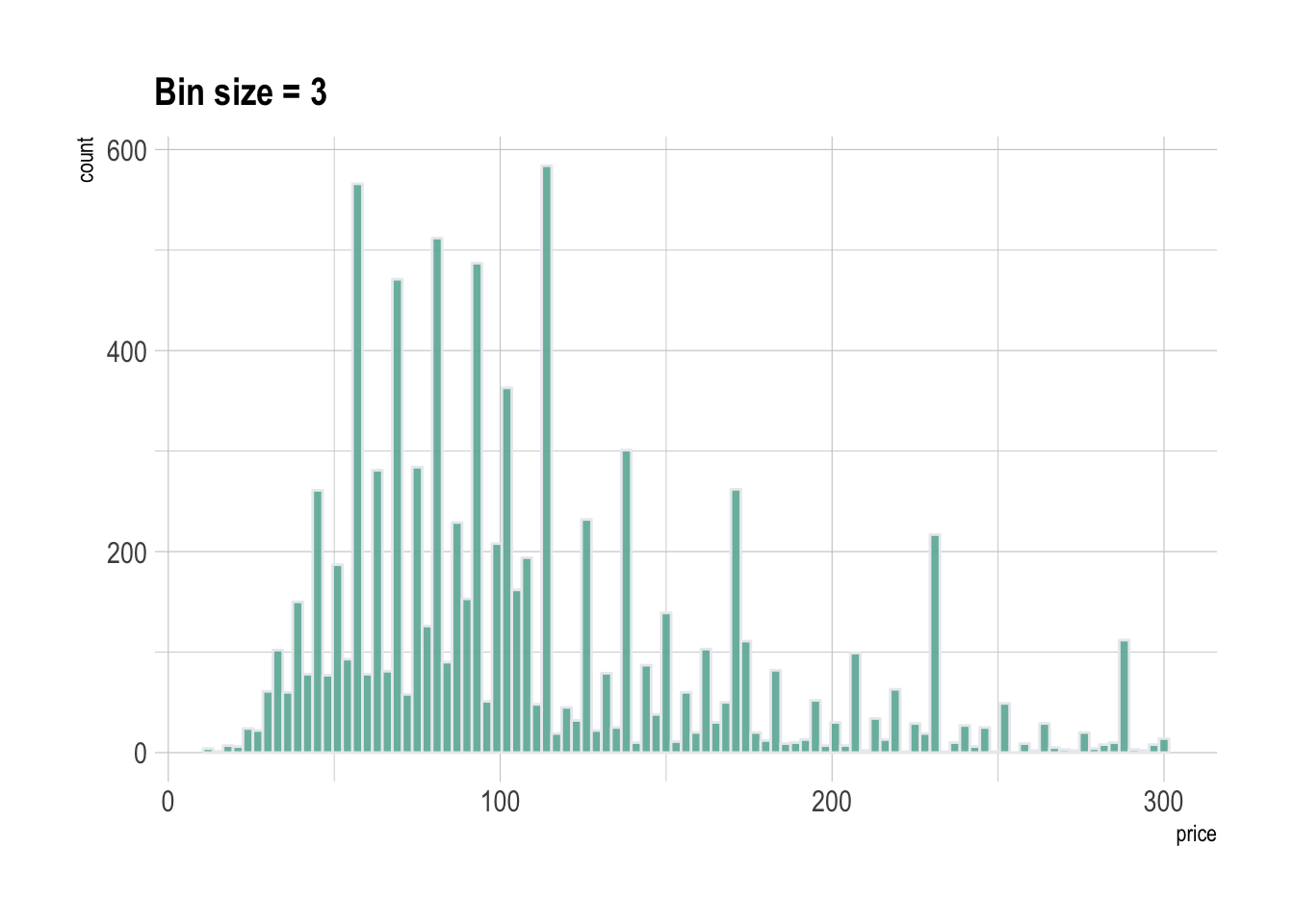
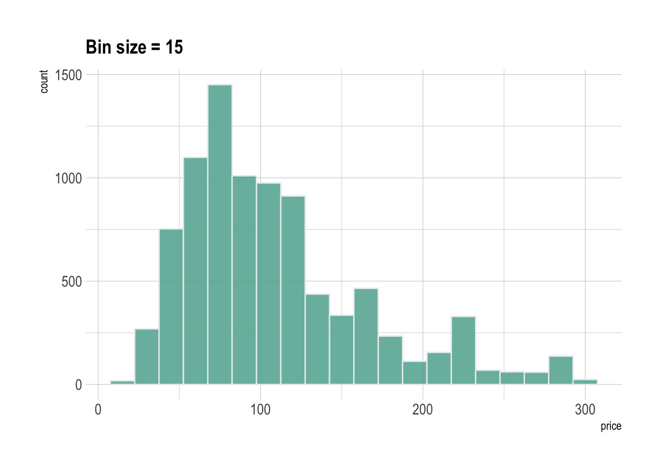
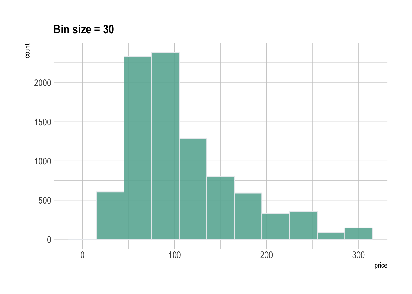
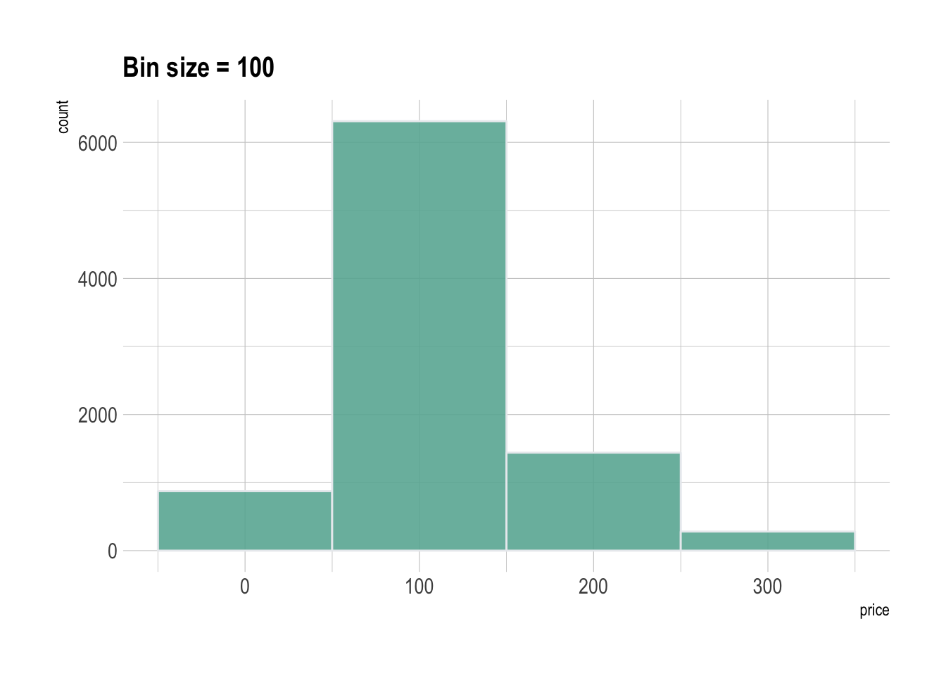
A histogram takes as input a numeric variable and cuts it into several bins. Playing with the bin size is a very important step, since its value can have a big impact on the histogram appearance and thus on the message you’re trying to convey. This concept is explained in depth in data-to-viz.
Ggplot2 makes it a breeze to change the bin size thanks to the binwidth argument of the geom_histogram function. See below the impact it can have on the output.
# Libraries
library(tidyverse)
library(hrbrthemes)

# Load dataset from github
data <- read.table("https://raw.githubusercontent.com/holtzy/data_to_viz/master/Example_dataset/1_OneNum.csv", header=TRUE)

# plot
p <- data %>%
  filter( price<300 ) %>%
  ggplot( aes(x=price)) +
    geom_histogram( binwidth=3, fill="#69b3a2", color="#e9ecef", alpha=0.9) +
    ggtitle("Bin size = 3") +
    theme_ipsum() +
    theme(
      plot.title = element_text(size=15)
    )
#p