Standardised vs. Non-Standardised
This page compares my reference standardised polygenic scores to non-reference standardised polygenic scores.
1 Original scores
Polygenic scores for UKB were derived using PRSice, genotyped SNPs only, including the MHC region, with LD-estimates from the UKB sample. My polygenic scores were derived without using the pT+clump method but not using PRSice, I used HapMap3 variants from the UKB imputed genetic data, I used only the single top SNP from the MHC region, and LD estimates from the EUR popultion in 1KG Phase 3.
Check the correlation between the two types of polygenic scores and how well they predict outcomes.
Show code
library(data.table)

pheno_name<-c('BMI','CAD','Intelligence','IBD','T2D','Height','RheuArth','MultiScler')
gwas<-c('BODY03','COAD01','COLL01','CROH01','DIAB05','HEIG03','RHEU01','SCLE02')

Results<-NULL
cor_res<-NULL
for(i in 1:length(gwas)){
  PRS_geno<-fread(paste0('/mnt/lustre/groups/ukbiobank/sumstats/PRS/ukb18177_glanville/PRS_for_use/',gwas[i],'_header.all.score'))
  PRS_stand<-fread(paste0('/users/k1806347/brc_scratch/Data/UKBB/PRS_for_comparison/1KG_ref/pt_clump/',gwas[i],'/UKBB.subset.w_hm3.',gwas[i],'.profiles'))
  PRS_geno$FID<-NULL
  PRS_stand$FID<-NULL

  # Extract individuals in common between the two PRSs
  overlap<-intersect(PRS_geno$IID, PRS_stand$IID)
  PRS_geno<-PRS_geno[PRS_geno$IID %in% overlap,]
  PRS_stand<-PRS_stand[PRS_stand$IID %in% overlap,]

  # Extract individuals surviving QC
  keep<-fread('/users/k1806347/brc_scratch/Analyses/PRS_comparison/UKBB_outcomes_for_prediction/ukb18177_glanville_post_qc_id_list.UpdateIDs.fam')
  PRS_geno<-PRS_geno[PRS_geno$IID %in% keep$V2,]
  PRS_stand<-PRS_stand[PRS_stand$IID %in% keep$V2,]

  # Extract pTs in common
  overlap_pT<-intersect(names(PRS_stand), names(PRS_geno))
  pTs<-overlap_pT[grepl(gwas[i], overlap_pT)]
  PRS_geno<-PRS_geno[,names(PRS_geno) %in% overlap_pT, with=F]
  PRS_stand<-PRS_stand[,names(PRS_stand) %in% overlap_pT, with=F]

  # Read in the phenotype file
  pheno<-fread(paste0('/users/k1806347/brc_scratch/Data/UKBB/Phenotype/PRS_comp_subset/UKBB.',pheno_name[i],'.txt'))
  pheno$FID<-NULL
  pheno_var<-names(pheno)[2]

  # Merge pheno and PRS
  PRS_geno_pheno<-merge(pheno, PRS_geno, by='IID')
  PRS_stand_pheno<-merge(pheno, PRS_stand, by='IID')

  # Run regressions
  for(k in 1:length(pTs)){
    geno_PRS_mod<-lm(as.formula(paste0('scale(',pheno_var,') ~ scale(',pTs[k],')')), data=PRS_geno_pheno)
    geno_PRS_mod_summary<-summary(geno_PRS_mod)
    stand_PRS_mod<-lm(as.formula(paste0('scale(',pheno_var,') ~ scale(',pTs[k],')')), data=PRS_stand_pheno)
    stand_PRS_mod_summary<-summary(stand_PRS_mod)

    Results<-rbind(Results, data.frame( Phenotype=rep(pheno_name[i],2),
                                        pT=rep(gsub(paste0(gwas[i],'_'),'',pTs[k]),2),
                                        Type=c('Current   ','Standardised'),
                                        BETA=c(coef(geno_PRS_mod_summary)[2,1],coef(stand_PRS_mod_summary)[2,1]),
                                        SE=c(coef(geno_PRS_mod_summary)[2,2],coef(stand_PRS_mod_summary)[2,2])))
  }

  # Calculate correlation between the two PRS
  names(PRS_stand)[-1]<-paste0(names(PRS_stand),'_geno')[-1]
  prs_both<-merge(PRS_geno,PRS_stand,by='IID')

  pT<-gsub('.*_','',names(PRS_geno)[-1])

  for(k in pT){
    res<-cor(prs_both[[paste0(gwas[i],'_',k)]], prs_both[[paste0(gwas[i],'_',k,'_geno')]])
    cor_res<-rbind(cor_res, data.frame( GWAS=gwas[i],
                                                            pT=k,
                                        cor=res))
  }

  # Fit model with both PRS
  both_PRS_mod_pheno<-merge(pheno, prs_both, by='IID')

  for(k in 1:length(pTs)){
    both_PRS_mod<-lm(as.formula(paste0('scale(',pheno_var,') ~ scale(',pTs[k],') + scale(',pTs[k],'_geno)')), data=both_PRS_mod_pheno)

    both_PRS_mod_summary<-summary(lm(as.formula(paste0('scale(both_PRS_mod_pheno$',pheno_var,') ~ scale(predict(both_PRS_mod, newdata = both_PRS_mod_pheno))'))))

    Results<-rbind(Results, data.frame( Phenotype=pheno_name[i],
                                        pT=gsub(paste0(gwas[i],'_'),'',pTs[k]),
                                        Type=c('Both   '),
                                        BETA=coef(both_PRS_mod_summary)[2,1],
                                        SE=coef(both_PRS_mod_summary)[2,2]))
  }

}

# Plot the results
library(ggplot2)
library(cowplot)

Plots<-list()
for(i in 1:length(gwas)){
Plots[[pheno_name[i]]]<-ggplot(Results[Results$Phenotype == pheno_name[i],], aes(x=pT, y=BETA, fill=Type)) +
                        geom_bar(position=position_dodge(), stat="identity") +
                        geom_errorbar(aes(ymin=BETA-SE, ymax=BETA+SE), width=.2, position=position_dodge(.9)) +
                        labs(title=pheno_name[i], y='Correlation', x=paste0('pT for ',gwas[i],' PRS')) +
                        theme(axis.text.x = element_text(angle = 45, hjust = 1), legend.position = 'top', legend.justification = c(0.5, 0), legend.title=element_blank())
}

png('/users/k1806347/brc_scratch/Analyses/PRS_comparison/UKBB_outcomes_for_prediction/Current_PRS_vs_standardised_PRS.png', unit='px', width=2000, height=3500, res=300)
plot_grid(plotlist=Plots, labels = "AUTO", ncol=2)
dev.off()

write.csv(cor_res, '/users/k1806347/brc_scratch/Analyses/PRS_comparison/UKBB_outcomes_for_prediction/Current_PRS_vs_standardised_PRS_cor.csv', row.names=F, quote=F)
Show correlation between phenotype and different PRS
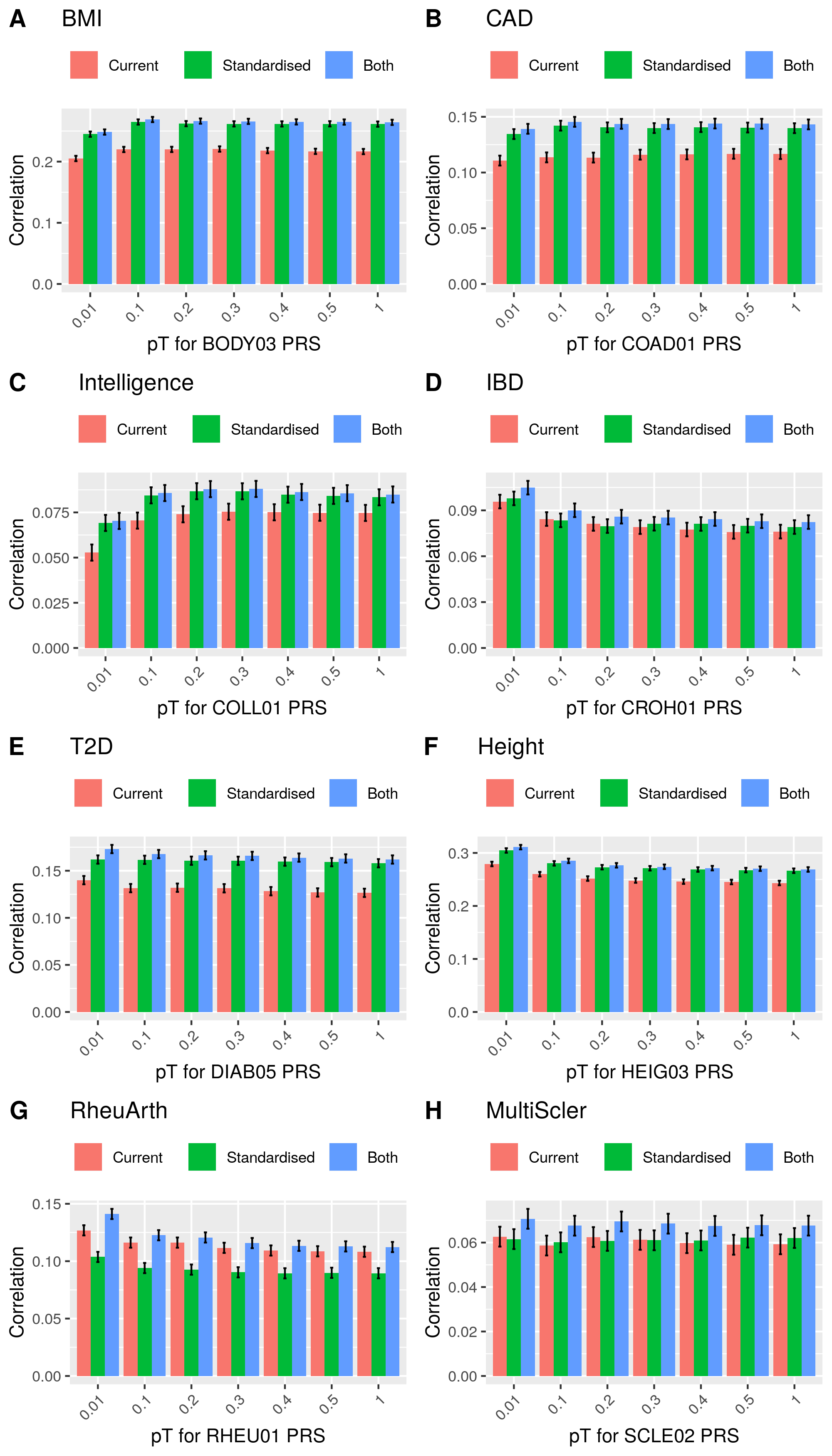
Correlation between phenotype and PRS
Show correlation between PRS
| GWAS | pT | cor |
|---|---|---|
| BODY03 | 0.01 | 0.7202845 |
| BODY03 | 0.10 | 0.7066447 |
| BODY03 | 0.20 | 0.7136640 |
| BODY03 | 0.30 | 0.7195138 |
| BODY03 | 0.40 | 0.7233397 |
| BODY03 | 0.50 | 0.7258802 |
| BODY03 | 1.00 | 0.7270496 |
| COAD01 | 0.01 | 0.6116274 |
| COAD01 | 0.10 | 0.6273054 |
| COAD01 | 0.20 | 0.6441036 |
| COAD01 | 0.30 | 0.6574784 |
| COAD01 | 0.40 | 0.6656764 |
| COAD01 | 0.50 | 0.6673727 |
| COAD01 | 1.00 | 0.6694118 |
| COLL01 | 0.01 | 0.6222449 |
| COLL01 | 0.10 | 0.7127647 |
| COLL01 | 0.20 | 0.7431230 |
| COLL01 | 0.30 | 0.7562313 |
| COLL01 | 0.40 | 0.7642572 |
| COLL01 | 0.50 | 0.7685698 |
| COLL01 | 1.00 | 0.7729352 |
| CROH01 | 0.01 | 0.7065433 |
| CROH01 | 0.10 | 0.7361608 |
| CROH01 | 0.20 | 0.7564487 |
| CROH01 | 0.30 | 0.7694719 |
| CROH01 | 0.40 | 0.7747197 |
| CROH01 | 0.50 | 0.7781611 |
| CROH01 | 1.00 | 0.7811400 |
| DIAB05 | 0.01 | 0.5495322 |
| DIAB05 | 0.10 | 0.5899781 |
| DIAB05 | 0.20 | 0.6086436 |
| DIAB05 | 0.30 | 0.6163363 |
| DIAB05 | 0.40 | 0.6209179 |
| DIAB05 | 0.50 | 0.6234401 |
| DIAB05 | 1.00 | 0.6255095 |
| HEIG03 | 0.01 | 0.7915908 |
| HEIG03 | 0.10 | 0.8224246 |
| HEIG03 | 0.20 | 0.8319358 |
| HEIG03 | 0.30 | 0.8354708 |
| HEIG03 | 0.40 | 0.8387046 |
| HEIG03 | 0.50 | 0.8398742 |
| HEIG03 | 1.00 | 0.8404782 |
| RHEU01 | 0.01 | 0.3635614 |
| RHEU01 | 0.10 | 0.5217018 |
| RHEU01 | 0.20 | 0.5668218 |
| RHEU01 | 0.30 | 0.5859811 |
| RHEU01 | 0.40 | 0.5971442 |
| RHEU01 | 0.50 | 0.6014540 |
| RHEU01 | 1.00 | 0.6055250 |
| SCLE02 | 0.01 | 0.5444079 |
| SCLE02 | 0.10 | 0.5444104 |
| SCLE02 | 0.20 | 0.5740674 |
| SCLE02 | 0.30 | 0.5922845 |
| SCLE02 | 0.40 | 0.5992493 |
| SCLE02 | 0.50 | 0.6052226 |
| SCLE02 | 1.00 | 0.6120867 |
The results show the PRS calcualted using these two approaches predict phenotypes to a similar degree, and although he scores are not highly correlated, their covariance with phenotypic data is higlighy correlated as a joint model does not improve prediction substantially.