---
author: "Mikhail Dozmorov, Ph.D."
institute: "https:/bit.ly/3Dgenomics"
date: "January 22, 2021"
output:
xaringan::moon_reader:
lib_dir: libs
css: ["css/xaringan-themer.css", "css/xaringan-my.css"]
nature:
ratio: '16:9'
highlightStyle: github
highlightLines: true
countIncrementalSlides: false
---
```{r xaringan-themer, include = FALSE}
library(xaringanthemer)
library(icons)
mono_light(
base_color = "midnightblue",
header_font_google = google_font("Noto Sans"),
text_font_google = google_font("Montserrat", "500", "500i"),
code_font_google = google_font("Droid Mono"),
link_color = "#8B1A1A", #firebrick4, "deepskyblue1"
text_font_size = "28px",
code_font_size = "26px"
)
```
class: center, middle
# The genome in action
### Detecting and interpreting changes in the 3D genome organization
[bit.ly/3Dgenomics](https://mdozmorov.github.io/Talk_3Dgenome/)
Mikhail Dozmorov, Ph.D.
Associate professor, Department of Biostatistics
Virginia Commonwealth University
---
## Overview
I. Normalization and differential analysis of Hi-C data
- HiCcompare
- multiHiCcompare
II. Detection and differential analysis of Topologically Associating Domains (TADs)
- SpectralTAD
- TADcompare
---
## The 3D structure of the genome
- Human genome is big - ~3.2 billion base pairs
- ~4 meters (~12ft) of diploid genome is packed into ~10um nucleus
- ~800 trips from Earth to Sun in ~30T cells from the human body
.center[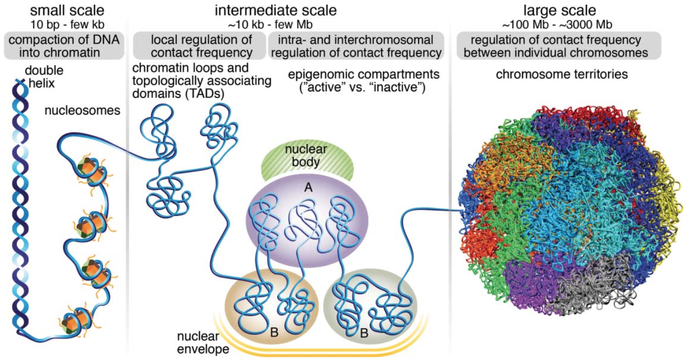 ]
]
Human body has approximately 30 trillion human cells (excluding trillions of microbiome cells); Stretched haploid genome would be roughly 2 meters - each cell has 4 meters of DNA (1 m = 3.28 ft); 30 trillion * 4 meters = 120 trillion meters; Convert to miles: 120 trillion meters / 1609.34 = 7.45*10^{10}; Convert to Earth-Sun distance: 7.45*10^{10} / 91.43*10^6 = 814.83
---
##The 3D genome is not static
- The 3D structure of the genome plays a role in many diseases
- Changes in the 3D genome organization are an ~~emerging~~ established hallmark of cancer
- Disruption of 3D genomic structure can lead to rewiring of enhancer-promoter interactions and changes in gene expression -> disease
---
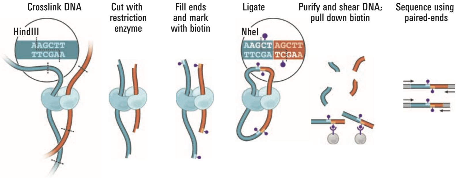
## Chromatin conformation capture technologies
.pull-left[
- 3C, 4C, 5C, Hi-C
- Capture-(Hi)C, ChIA-PET
- Single-cell variants
- SPRITE, GAM, ChIA-Drop
- Specialized (e.g., Methyl-HiC)
]
.pull-right[
]
.small[ Lieberman-Aiden, Erez et al. “[Comprehensive Mapping of Long-Range Interactions Reveals Folding Principles of the Human Genome](https://doi.org/10.1126/science.1181369)” _Science_, October 9, 2009 ]
---
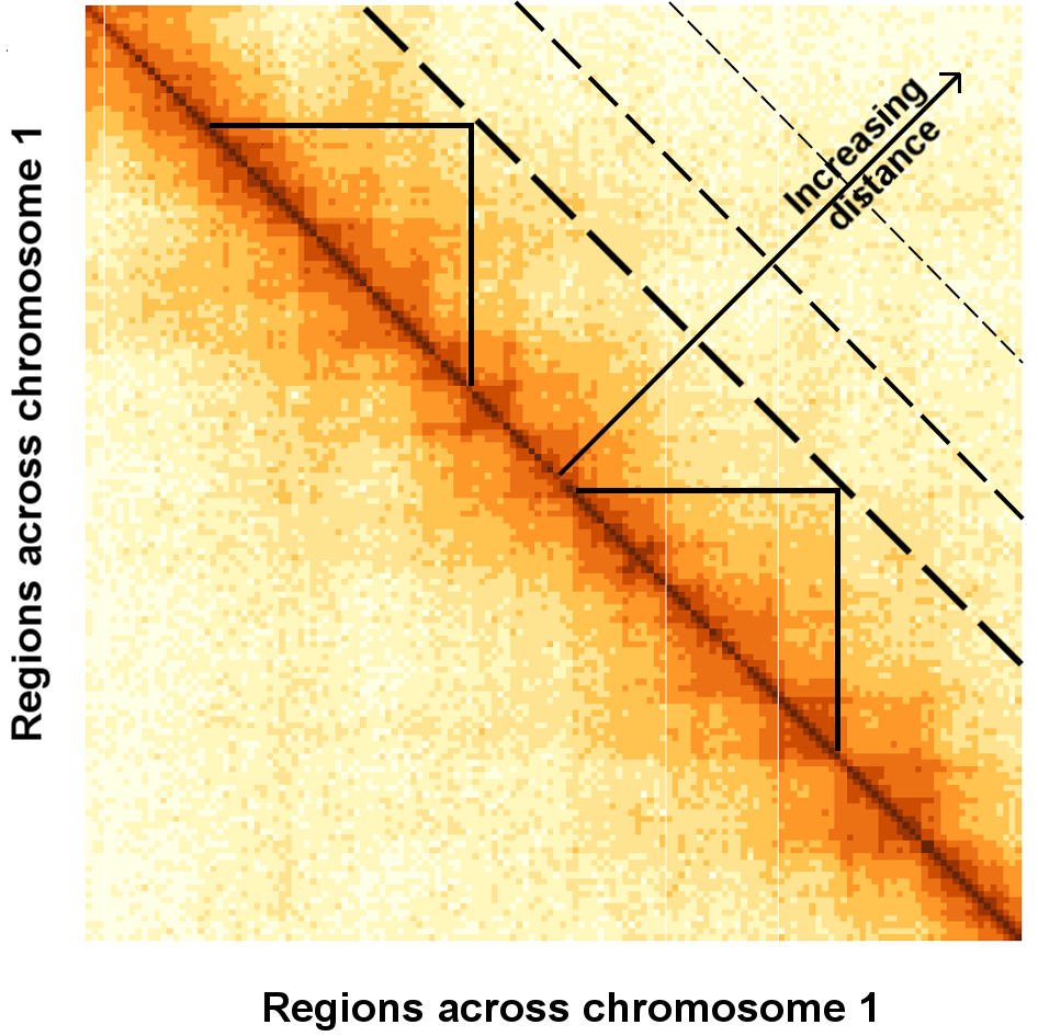
## Hi-C Data as a matrix
.pull-left[
- The genome (chromosome) is split into equally sized regions
- Data is represented by a symmetric matrix of contacts $C_{ij}$ where entry $ij$ corresponds to the number of times region $i$ comes into contact with region $j$
- Off-diagonal data view - increasing **distance** between interacting regions
- Power-law decay of interactions with increasing **distance**
]
.pull-right[
 ]
---
## Biases in Hi-C data
- Hi-C data suffers from many biases: **sequence-driven** (e.g., mappability, CG content) & **technology-driven** (e.g., type of restriction enzyme, sequencing platform)
- Most normalization methods work only on individual Hi-C dataset, one at a time
- Individual normalization methods do not perform well when the goal is comparison
---
class: center, middle
# HiCcompare
Joint normalization and differential analysis of Hi-C data
---
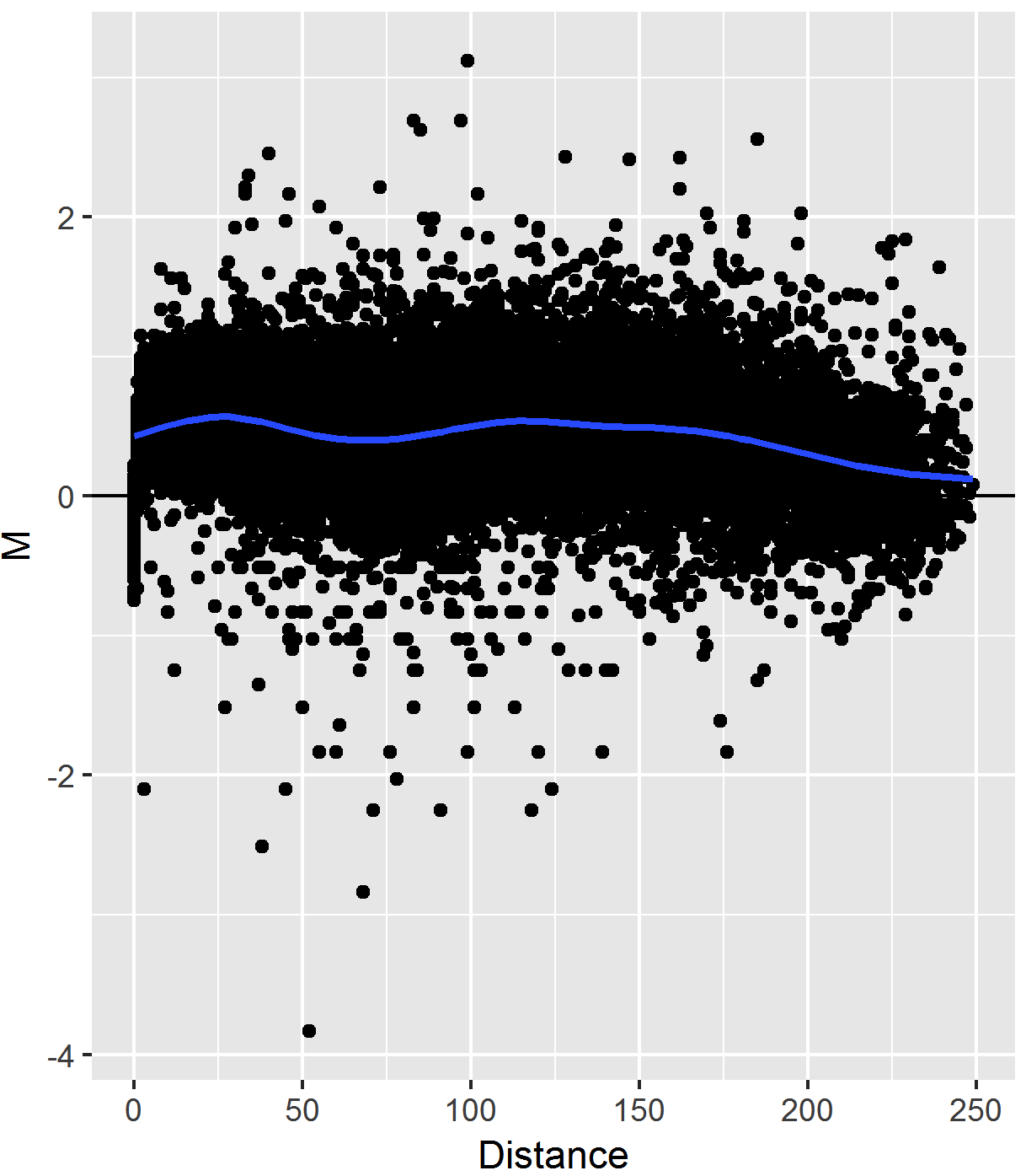
## Joint Normalization on the MD plot
.pull-left[
- **MD plot** represents data from two Hi-C matrices on one plot
- Similar to the MA plot (Bland-Altman plot)
- X-axis: **Genomic Distance** (off-diagonal data slices)
- Y-axis: **Mean differences in interaction frequencies** (log2(IF2/IF1))
]
.pull-right[
]
---
## Biases in Hi-C data
- Hi-C data suffers from many biases: **sequence-driven** (e.g., mappability, CG content) & **technology-driven** (e.g., type of restriction enzyme, sequencing platform)
- Most normalization methods work only on individual Hi-C dataset, one at a time
- Individual normalization methods do not perform well when the goal is comparison
---
class: center, middle
# HiCcompare
Joint normalization and differential analysis of Hi-C data
---
## Joint Normalization on the MD plot
.pull-left[
- **MD plot** represents data from two Hi-C matrices on one plot
- Similar to the MA plot (Bland-Altman plot)
- X-axis: **Genomic Distance** (off-diagonal data slices)
- Y-axis: **Mean differences in interaction frequencies** (log2(IF2/IF1))
]
.pull-right[
 ]
---
## Loess regression
.pull-left[
- Differences between two datasets should be minimal (symmetric around M = 0, Y-axis)
- Local Regression – fit based on local subsets of the data
- Nonlinear, data-driven - creates a smooth curve through the data
- Can use loess fit to correct for bias
]
.pull-right[
.center[
]
---
## Loess regression
.pull-left[
- Differences between two datasets should be minimal (symmetric around M = 0, Y-axis)
- Local Regression – fit based on local subsets of the data
- Nonlinear, data-driven - creates a smooth curve through the data
- Can use loess fit to correct for bias
]
.pull-right[
.center[ ]
]
---
## Joint Loess Normalization of Hi-C Data
.pull-left[
- Differences between two datasets should be minimal (symmetric around M = 0, Y-axis)
- Perform loess regression on the MD plot to calculate $f(D)$ - the predicted interaction frequency $IF$ value at distance $D$
.small[
- $log_2(\hat{IF_{1D}})=log_2(IF_{1D})-f(D)/2$
- $log_2(\hat{IF_{2D}})=log_2(IF_{2D})+f(D)/2$
- Average $IF$ for the pair remains unchanged
]
]
.pull-right[
.center[
]
]
---
## Joint Loess Normalization of Hi-C Data
.pull-left[
- Differences between two datasets should be minimal (symmetric around M = 0, Y-axis)
- Perform loess regression on the MD plot to calculate $f(D)$ - the predicted interaction frequency $IF$ value at distance $D$
.small[
- $log_2(\hat{IF_{1D}})=log_2(IF_{1D})-f(D)/2$
- $log_2(\hat{IF_{2D}})=log_2(IF_{2D})+f(D)/2$
- Average $IF$ for the pair remains unchanged
]
]
.pull-right[
.center[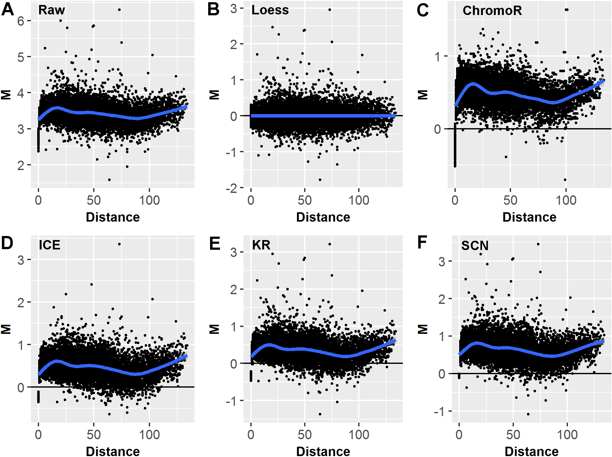 ]
]
.small[ Benchmarking study: Lyu, Hongqiang, Erhu Liu, and Zhifang Wu. “[Comparison of Normalization Methods for Hi-C Data](https://doi.org/10.2144/btn-2019-0105)” _BioTechniques_, October 7, 2019
]
---
## Difference detection
.pull-left[
- At each distance, take a set of M-values
- Convert M-values to Z-scores $Z_i=\frac{M_i-\hat{M}}{\sigma_M}$
- Z-scores are compared to standard normal distribution to obtain p-values
- FDR multiple testing correction applied on a per-distance basis
]
.pull-right[
.center[
]
]
.small[ Benchmarking study: Lyu, Hongqiang, Erhu Liu, and Zhifang Wu. “[Comparison of Normalization Methods for Hi-C Data](https://doi.org/10.2144/btn-2019-0105)” _BioTechniques_, October 7, 2019
]
---
## Difference detection
.pull-left[
- At each distance, take a set of M-values
- Convert M-values to Z-scores $Z_i=\frac{M_i-\hat{M}}{\sigma_M}$
- Z-scores are compared to standard normal distribution to obtain p-values
- FDR multiple testing correction applied on a per-distance basis
]
.pull-right[
.center[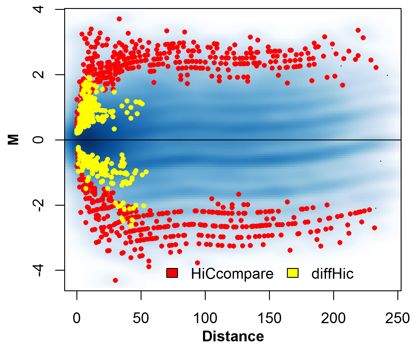 ]
]
---
## Difference Detection After Different Normalizations
.pull-left[
- Simulated 100x100 chromatin interaction matrices with 250 controlled changes applied
- ROC curves for different normalization techniques and fold changes
- Loess provides the most power to detect small fold changes
.small[ https://bioconductor.org/packages/HiCcompare/
Stansfield, John C., Kellen G. Cresswell, Vladimir I. Vladimirov, and Mikhail G. Dozmorov. “[HiCcompare: An R-Package for Joint Normalization and Comparison of HI-C Datasets](https://doi.org/10.1186/s12859-018-2288-x)” _BMC Bioinformatics_, December 2018 ]
]
.pull-right[
.center[
]
]
---
## Difference Detection After Different Normalizations
.pull-left[
- Simulated 100x100 chromatin interaction matrices with 250 controlled changes applied
- ROC curves for different normalization techniques and fold changes
- Loess provides the most power to detect small fold changes
.small[ https://bioconductor.org/packages/HiCcompare/
Stansfield, John C., Kellen G. Cresswell, Vladimir I. Vladimirov, and Mikhail G. Dozmorov. “[HiCcompare: An R-Package for Joint Normalization and Comparison of HI-C Datasets](https://doi.org/10.1186/s12859-018-2288-x)” _BMC Bioinformatics_, December 2018 ]
]
.pull-right[
.center[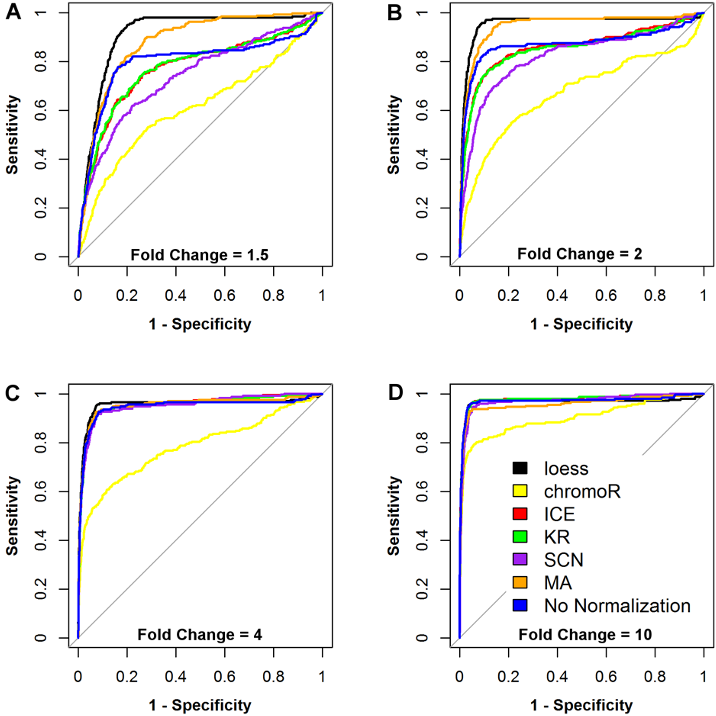 ]
]
---
class: center, middle
# multiHiCcompare
Normalization and differential analysis of multiple Hi-C datasets
---
## Normalization: Multiple Hi-C datasets
**Cyclic loess** (Ballman et al. 2004) to jointly normalize multiple datasets - take each pair of datasets, normalize, repeat until convergence
1. Choose two out of the N total samples, then generate an MD plot
2. Fit a loess curve $f(D)$ to the MD plot
3. Subtract $f(D)/2$ from the first dataset and add $f(D)/2$ to the second
4. Repeat until all unique pairs have been compared
5. Repeat until convergence
]
]
---
class: center, middle
# multiHiCcompare
Normalization and differential analysis of multiple Hi-C datasets
---
## Normalization: Multiple Hi-C datasets
**Cyclic loess** (Ballman et al. 2004) to jointly normalize multiple datasets - take each pair of datasets, normalize, repeat until convergence
1. Choose two out of the N total samples, then generate an MD plot
2. Fit a loess curve $f(D)$ to the MD plot
3. Subtract $f(D)/2$ from the first dataset and add $f(D)/2$ to the second
4. Repeat until all unique pairs have been compared
5. Repeat until convergence
.small[Ballman, Karla V., Diane E. Grill, Ann L. Oberg, and Terry M. Therneau. “[Faster Cyclic Loess: Normalizing RNA Arrays via Linear Models](https://doi.org/10.1093/bioinformatics/bth327).” Bioinformatics (Oxford, England) 20, no. 16 (November 1, 2004)]
---
## Differential analysis: Multiple Hi-C datasets
- **Distance-centric analysis** – each off-diagonal data slice has unique statistical properties
- Split Hi-C data into $d$ distance-centric matrices with $g$ rows (indices for interacting pairs of regions) and $i$ columns (samples)
.center[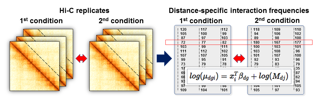 ]
---
## Differential analysis: Multiple Hi-C datasets
- Statistical framework of differential gene expression analysis can be adapted for differential analysis of IFs ([edgeR](https://bioconductor.org/packages/edgeR/) R package)
- **Exact test**
.small[
- For comparing 2 groups without other covariates
- Similar to Fisher's exact test
- Computes exact p-values by summing over all sums of counts that have a probability less than the probability under the null hypothesis
]
- **Generalized Linear Models**
.small[
- For more complex experiments, utilize the GLM framework
- The IF value for a pair of regions $g$ at distance $d$ from sample $i$ follows $NB(M_{di}*p_{dgj},\phi_{dg})$, where $M_{di}$ is the total number of reads in sample $i$ at distance $d$, $p_{dgj}$ is the proportion of interaction counts $g$ in sample $i$ from experimental condition $j$, $\phi_{dg}$ is the dispersion
- The vector of covariates $x_i$ can be linked with $\mu_{dgj}$ through a log-linear model $log(\mu_{dgj}) = x_i^T\beta_{dg} + log(M_{dj})$
]
---
## Analysis overview: Multiple Hi-C datasets
.center[
]
---
## Differential analysis: Multiple Hi-C datasets
- Statistical framework of differential gene expression analysis can be adapted for differential analysis of IFs ([edgeR](https://bioconductor.org/packages/edgeR/) R package)
- **Exact test**
.small[
- For comparing 2 groups without other covariates
- Similar to Fisher's exact test
- Computes exact p-values by summing over all sums of counts that have a probability less than the probability under the null hypothesis
]
- **Generalized Linear Models**
.small[
- For more complex experiments, utilize the GLM framework
- The IF value for a pair of regions $g$ at distance $d$ from sample $i$ follows $NB(M_{di}*p_{dgj},\phi_{dg})$, where $M_{di}$ is the total number of reads in sample $i$ at distance $d$, $p_{dgj}$ is the proportion of interaction counts $g$ in sample $i$ from experimental condition $j$, $\phi_{dg}$ is the dispersion
- The vector of covariates $x_i$ can be linked with $\mu_{dgj}$ through a log-linear model $log(\mu_{dgj}) = x_i^T\beta_{dg} + log(M_{dj})$
]
---
## Analysis overview: Multiple Hi-C datasets
.center[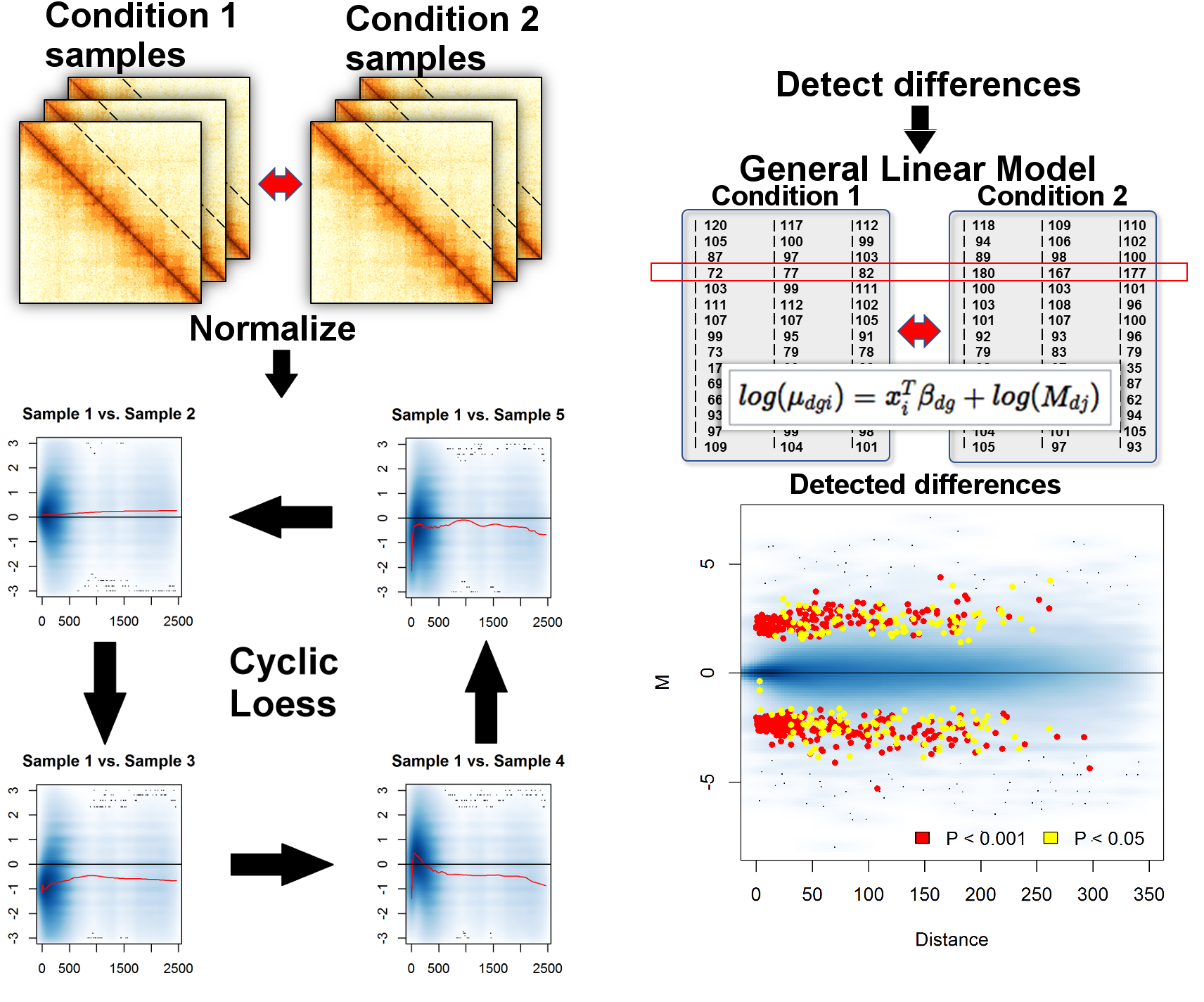 ]
.small[
Benchmarking study: Zheng, Ye, Peigen Zhou, and Sündüz Keleş. “[FreeHi-C Spike-in Simulations for Benchmarking Differential Chromatin Interaction Detection](https://doi.org/10.1016/j.ymeth.2020.07.001)” _Methods_, July 12, 2020
]
---
## Benchmarking
.center[
]
.small[
Benchmarking study: Zheng, Ye, Peigen Zhou, and Sündüz Keleş. “[FreeHi-C Spike-in Simulations for Benchmarking Differential Chromatin Interaction Detection](https://doi.org/10.1016/j.ymeth.2020.07.001)” _Methods_, July 12, 2020
]
---
## Benchmarking
.center[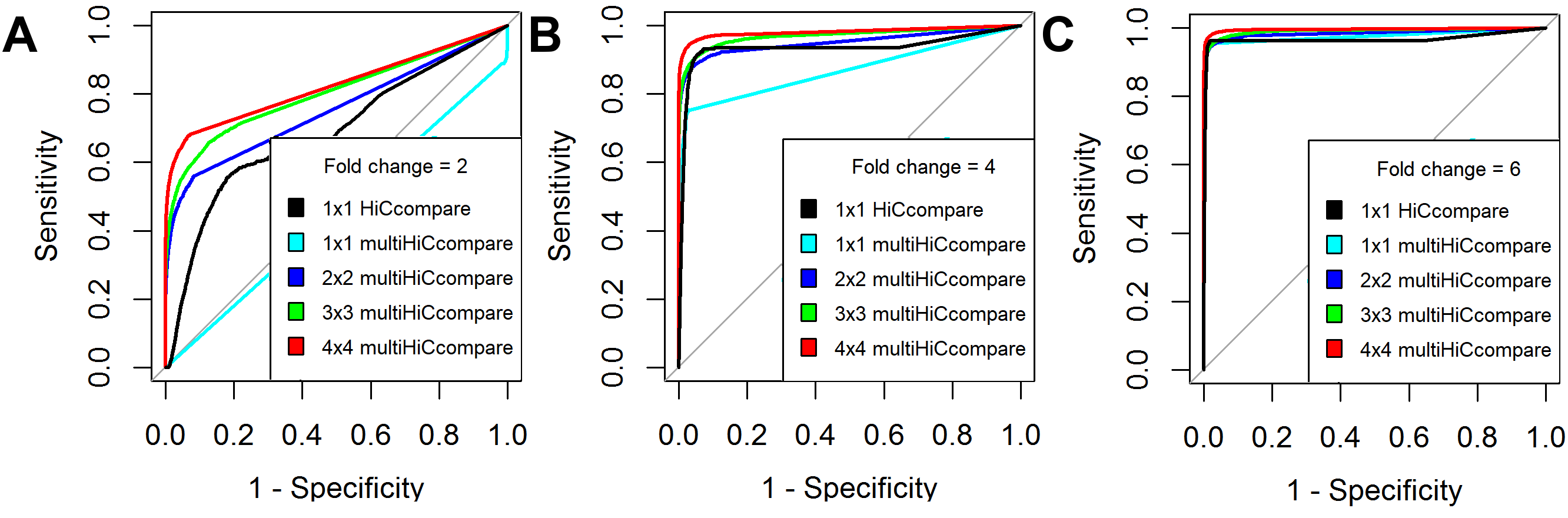 ]
.small[ https://bioconductor.org/packages/multiHiCcompare/
Stansfield, John C, Kellen G Cresswell, and Mikhail G Dozmorov. “[MultiHiCcompare: Joint Normalization and Comparative Analysis of Complex Hi-C Experiments](https://doi.org/10.1093/bioinformatics/btz048).” Bioinformatics, January 22, 2019 ]
---
class: center, middle
# SpectralTAD
Detection of Topologically Associating Domains using Spectral Clustering
---
## Topologically Associating Domains
- TADs are 3D structures of frequently interacting regions
- Boundaries are associated with specific genomic features (CTCF, cohesin, mediator)
- Can be hierarchical (nested, TADs containing sub-TADs)
.center[
]
.small[ https://bioconductor.org/packages/multiHiCcompare/
Stansfield, John C, Kellen G Cresswell, and Mikhail G Dozmorov. “[MultiHiCcompare: Joint Normalization and Comparative Analysis of Complex Hi-C Experiments](https://doi.org/10.1093/bioinformatics/btz048).” Bioinformatics, January 22, 2019 ]
---
class: center, middle
# SpectralTAD
Detection of Topologically Associating Domains using Spectral Clustering
---
## Topologically Associating Domains
- TADs are 3D structures of frequently interacting regions
- Boundaries are associated with specific genomic features (CTCF, cohesin, mediator)
- Can be hierarchical (nested, TADs containing sub-TADs)
.center[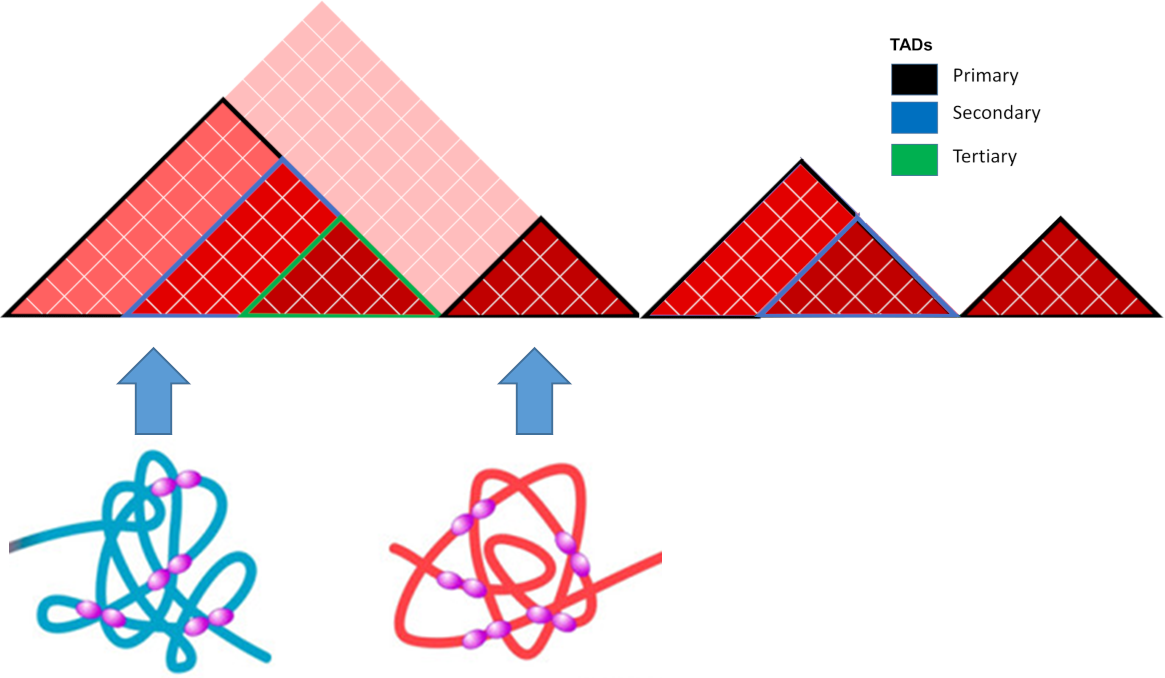 ]
---
## Why are TADs Important?
- Established early in development
- Highly correlate with replication timing
- TADs create "autonomous gene-domains" partitioning the genome into discrete functional regions
- Disruptions of TADs lead to _de novo_ enhancer-promoter interactions and dysregulation of gene expression -> disease
TADs are a distinct layer of the 3D genome organization
---
## TAD detection using graph theory
.pull-left[
- Hi-C data has a natural graph structure, defined by vertices $V$ and edges $E$
- **Vertices** are genomic regions
- **Edges** represent interaction strength between any pair of regions
- Vertices and edges are stored in an **adjacency matrix** $A_{ij}$ where $ij$ is the number of edges between a given set of vertices $ij$
]
.pull-right[ .center[
]
---
## Why are TADs Important?
- Established early in development
- Highly correlate with replication timing
- TADs create "autonomous gene-domains" partitioning the genome into discrete functional regions
- Disruptions of TADs lead to _de novo_ enhancer-promoter interactions and dysregulation of gene expression -> disease
TADs are a distinct layer of the 3D genome organization
---
## TAD detection using graph theory
.pull-left[
- Hi-C data has a natural graph structure, defined by vertices $V$ and edges $E$
- **Vertices** are genomic regions
- **Edges** represent interaction strength between any pair of regions
- Vertices and edges are stored in an **adjacency matrix** $A_{ij}$ where $ij$ is the number of edges between a given set of vertices $ij$
]
.pull-right[ .center[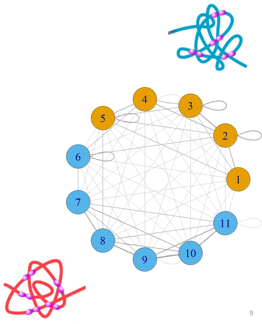 ]
]
]
---
## Traditional Spectral Clustering
- Specifically designed to cluster graphs
- Works by projecting the data into a lower-dimensional space
- Excels on noisy and non-normally distributed data (Hi-C data)
---
## How to perform spectral clustering
- Calculate the Laplacian:
$$D = diag(A\mathbf{1_n})$$
$$\bar{L} = D^{-\frac{1}{2}}AD^{-\frac{1}{2}}$$
- Calculate the eigenvectors of the Laplacian matrix (graph spectrum):
$$\bar{L}\mathbf{v} = \lambda\mathbf{v}$$
- Normalize the eigenvectors and cluster
---
## Spectral clustering with eigenvector gaps
- Rows and columns of Hi-C matrices are naturally ordered
- TADs are continuous
- Order points (genomic regions) in eigenvector space, and cluster
- We propose a simple, novel approach to clustering ordered data using gaps between consecutive points in eigenvector space
---
## Step 1: Plot the non-normalized eigenvectors
.center[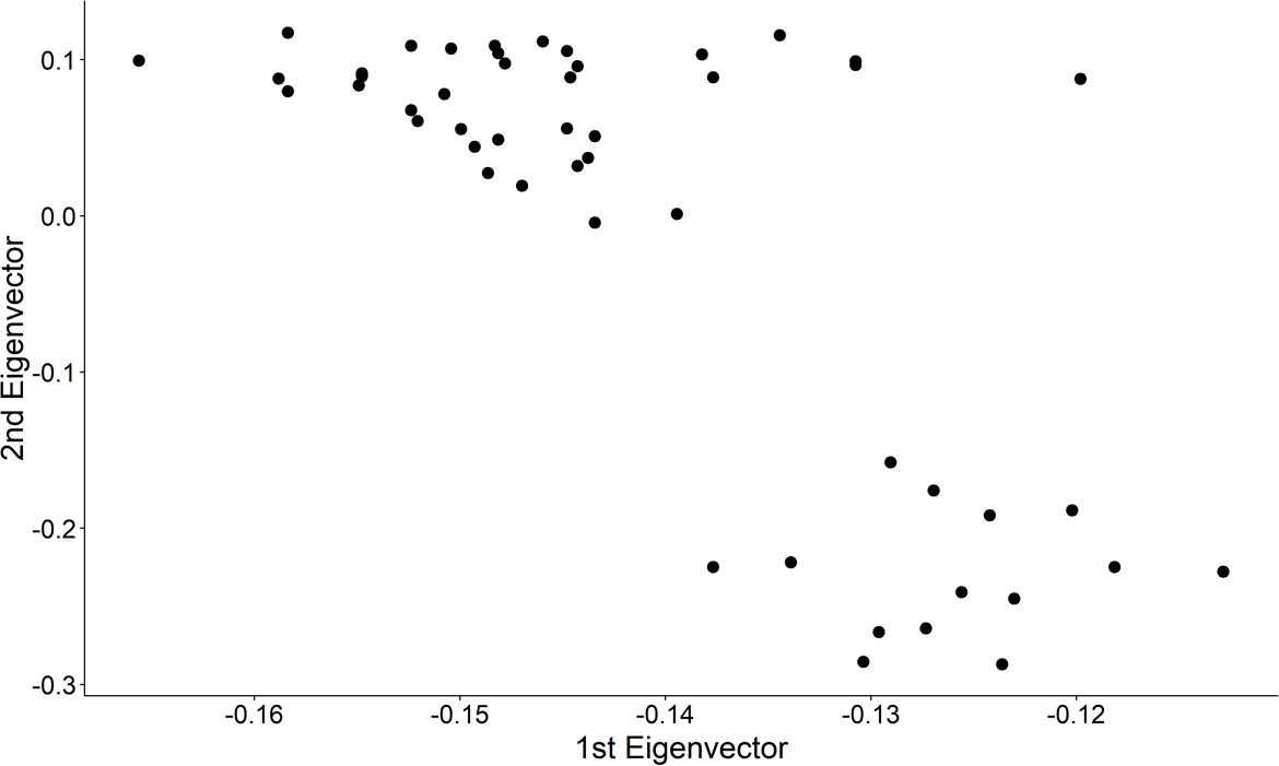 ]
---
## Step 2: Project on to Unit Circle
.center[
]
---
## Step 2: Project on to Unit Circle
.center[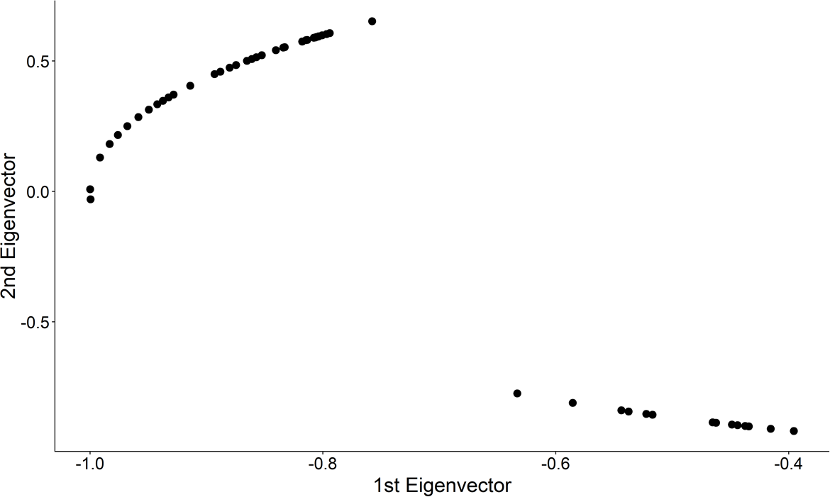 ]
---
## Step 3: Find the k-largest gaps and partition
.center[
]
---
## Step 3: Find the k-largest gaps and partition
.center[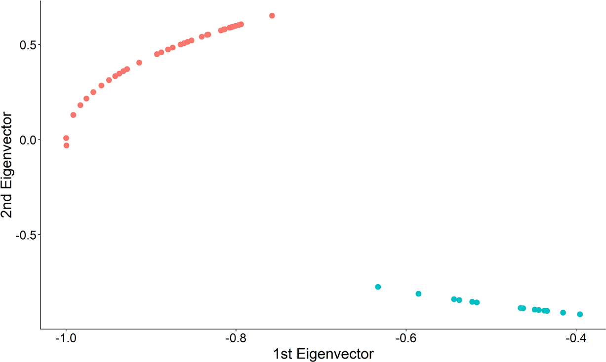 ]
---
## Step 3: Find the k-largest gaps and partition
.center[
]
---
## Step 3: Find the k-largest gaps and partition
.center[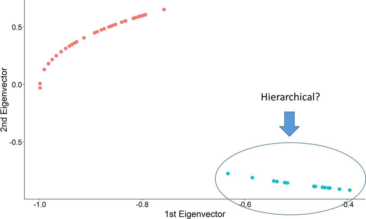 ]
---
## Windowed Spectral Clustering
- We know the biologically maximum TAD size (2 million bp)
- We can use a 2 million bp sliding window to perform spectral clustering and aggregate
- Advantages of the sliding window
- Reduced cubic complexity of spectral clustering $O(n^{3})$ to linear complexity $O(n)$
- Naturally discards noisy interactions at large genomic distances
---
## SpectralTAD algorithm
1. Cut a window from the matrix equal to the maximum TAD size (2Mb)
2. Find the graph spectrum of the window and calculate eigenvector gaps
3. Find a set of clusters that maximize the silhouette score
4. Slide the window to the next group of loci and repeat
.center[
]
---
## Windowed Spectral Clustering
- We know the biologically maximum TAD size (2 million bp)
- We can use a 2 million bp sliding window to perform spectral clustering and aggregate
- Advantages of the sliding window
- Reduced cubic complexity of spectral clustering $O(n^{3})$ to linear complexity $O(n)$
- Naturally discards noisy interactions at large genomic distances
---
## SpectralTAD algorithm
1. Cut a window from the matrix equal to the maximum TAD size (2Mb)
2. Find the graph spectrum of the window and calculate eigenvector gaps
3. Find a set of clusters that maximize the silhouette score
4. Slide the window to the next group of loci and repeat
.center[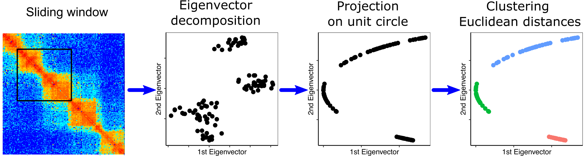 ]
---
## Determining a hierarchy of TADs
- TADs are hierarchical in nature (organized into large meta-TADs with sub-TADs within them)
- To find sub-TADs, we use a novel metric called boundary score
- **Boundary score** is just the z-score for each eigenvector gap (Euclidean distance between adjacent points)
.center[]
---
## Boundary score as a metric for TAD boundary detection
.center[
]
---
## Determining a hierarchy of TADs
- TADs are hierarchical in nature (organized into large meta-TADs with sub-TADs within them)
- To find sub-TADs, we use a novel metric called boundary score
- **Boundary score** is just the z-score for each eigenvector gap (Euclidean distance between adjacent points)
.center[]
---
## Boundary score as a metric for TAD boundary detection
.center[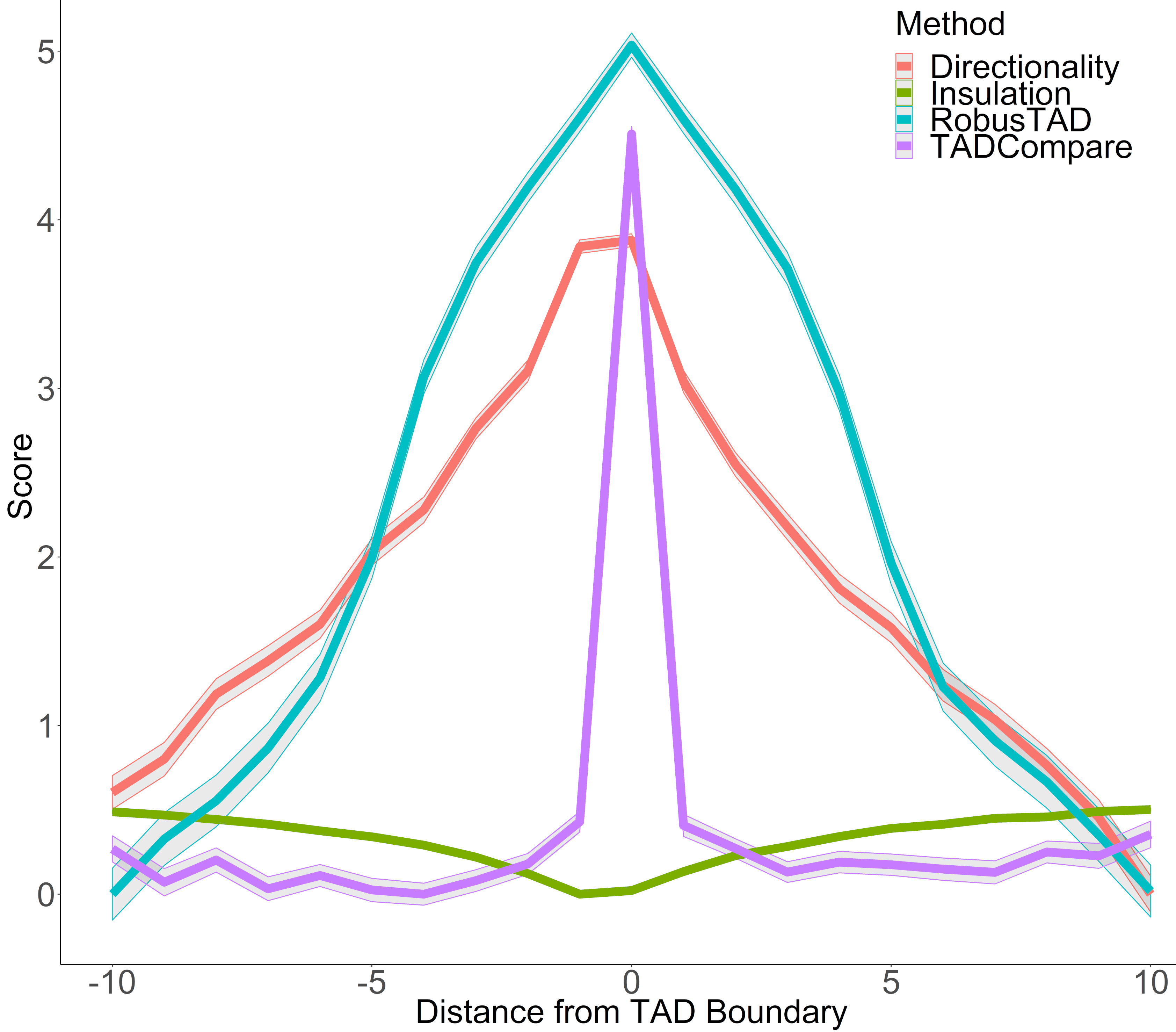 ]
---
## Determining a hierarchy of TADs
For each initial TAD:
- Perform spectral clustering on the submatrix defined by the initial TAD
- Calculate the eigenvector gaps for each consecutive pair of regions
- Convert eigenvector gaps to boundary scores
- If any boundary score is greater than 1.96, this is a sub-TAD boundary
- Repeat for all sub-TADs until no z-score is greater than 1.96
---
## TAD Calling: SpectralTAD
- We compared SpectralTAD against four TAD callers:
- TopDom
- HiCSeg
- OnTAD
- rGMAP
- Good TAD caller must satisfy three criteria:
- Be robust to Hi-C data imperfections (resolution, sparsity, sequencing depth)
- Detect biologically significant, hierarchical TAD boundaries
- Be fast
---
## SpectralTAD is robust to resolution
.center[
]
---
## Determining a hierarchy of TADs
For each initial TAD:
- Perform spectral clustering on the submatrix defined by the initial TAD
- Calculate the eigenvector gaps for each consecutive pair of regions
- Convert eigenvector gaps to boundary scores
- If any boundary score is greater than 1.96, this is a sub-TAD boundary
- Repeat for all sub-TADs until no z-score is greater than 1.96
---
## TAD Calling: SpectralTAD
- We compared SpectralTAD against four TAD callers:
- TopDom
- HiCSeg
- OnTAD
- rGMAP
- Good TAD caller must satisfy three criteria:
- Be robust to Hi-C data imperfections (resolution, sparsity, sequencing depth)
- Detect biologically significant, hierarchical TAD boundaries
- Be fast
---
## SpectralTAD is robust to resolution
.center[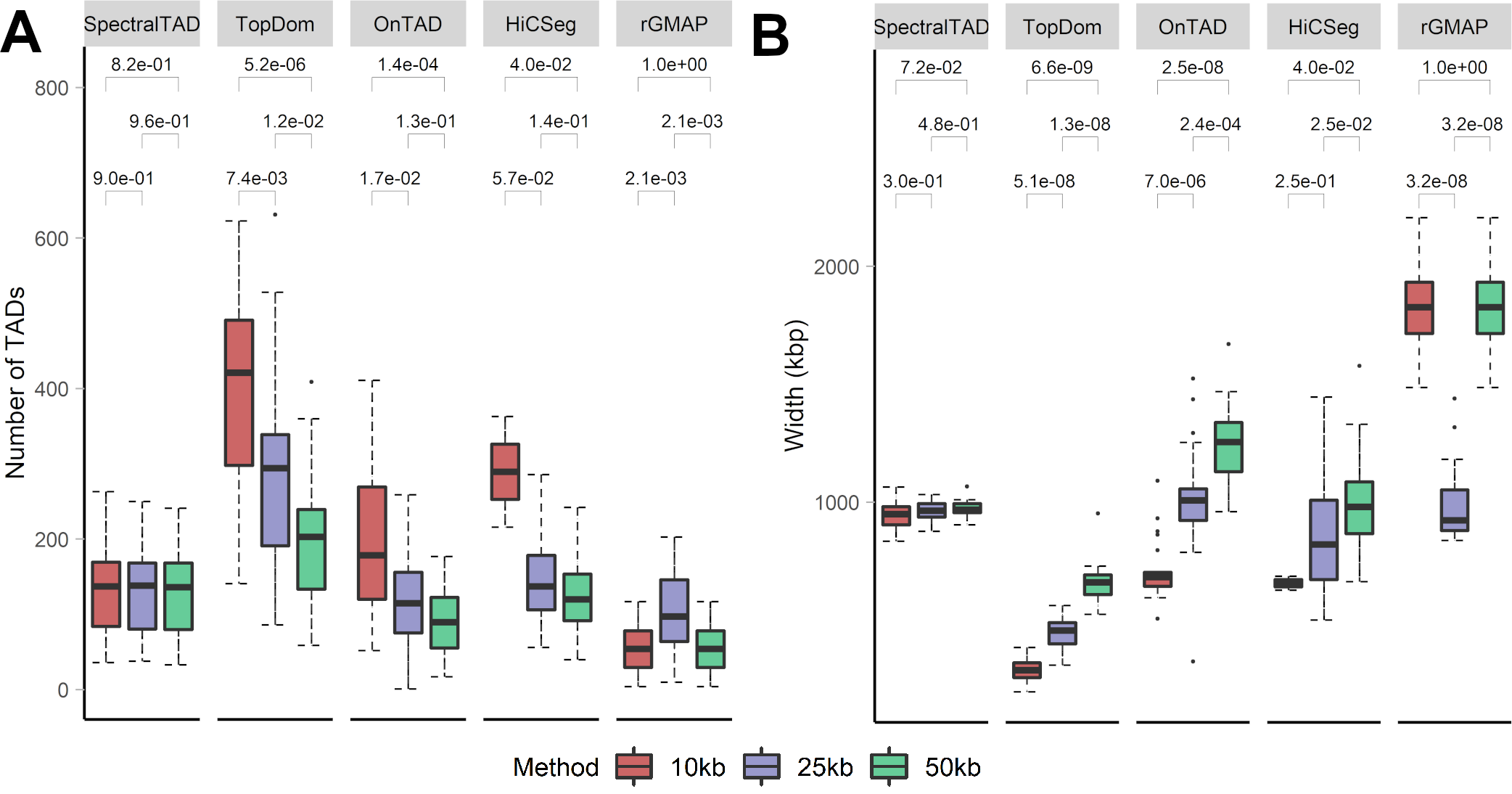 ]
---
## SpectralTAD is robust to sparsity
- 25 simulated matrices with pre-defined TADs (HiCToolsCompare)
- The percentage of the matrix replaced with zeros
- Jaccard similarity between the detected and pre-defined TADs
.center[
]
---
## SpectralTAD is robust to sparsity
- 25 simulated matrices with pre-defined TADs (HiCToolsCompare)
- The percentage of the matrix replaced with zeros
- Jaccard similarity between the detected and pre-defined TADs
.center[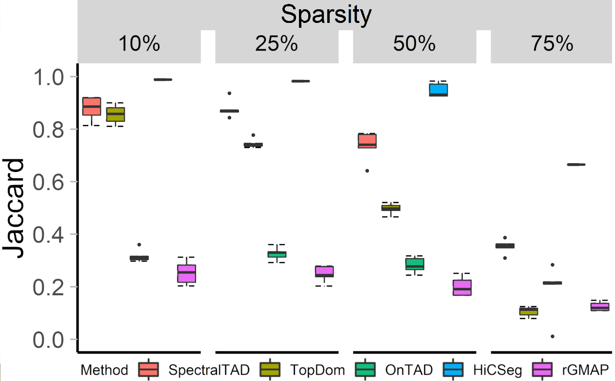 ]
---
## SpectralTAD is robust to sequencing depth
- Downsample matrices uniformly at random
- Measure Jaccard similarity between TADs detected from the original and sparse data
.center[
]
---
## SpectralTAD is robust to sequencing depth
- Downsample matrices uniformly at random
- Measure Jaccard similarity between TADs detected from the original and sparse data
.center[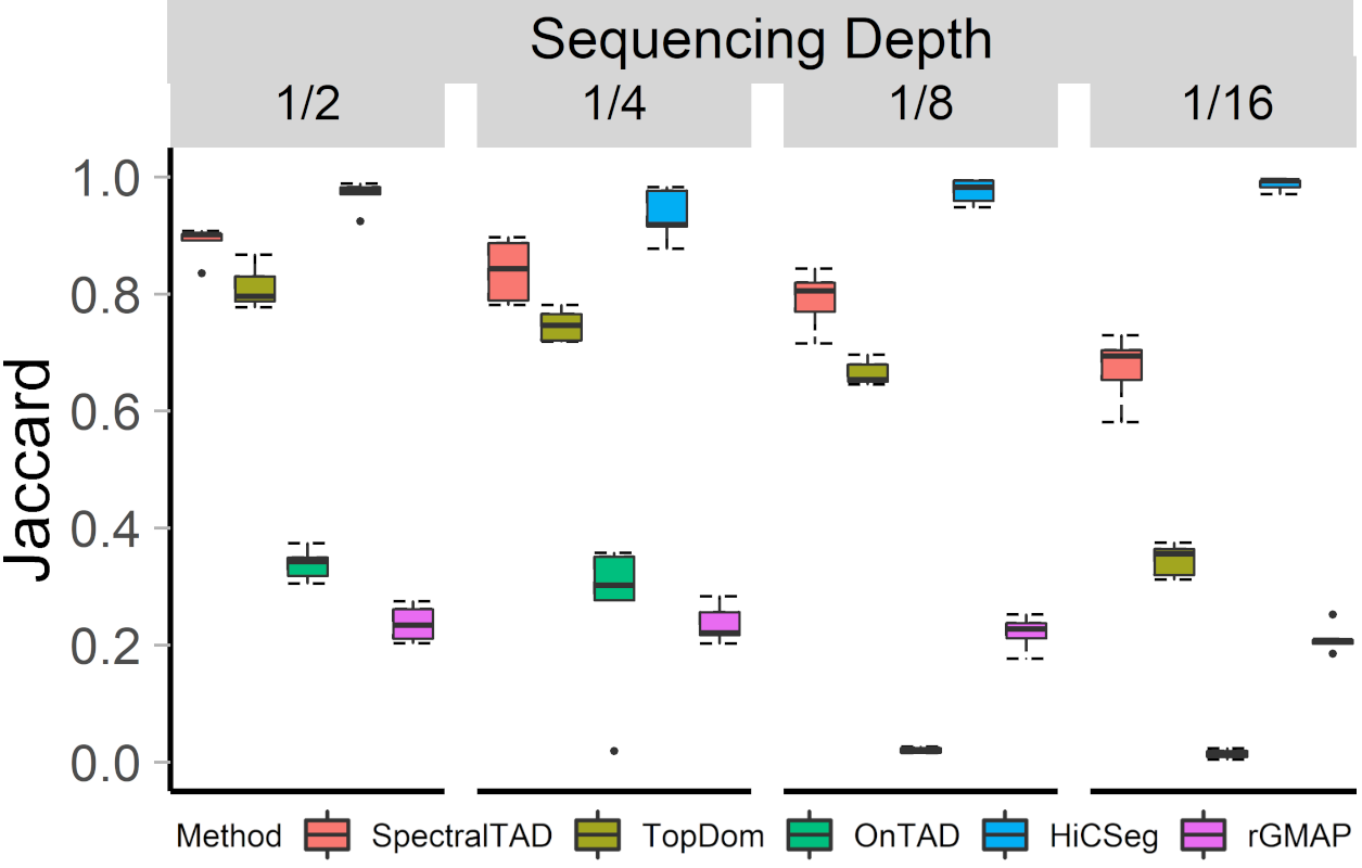 ]
---
## Hierarchical TAD boundaries differ
- Boundaries shared by two TADs (Level 2) or three TADs (Level 3) are more biologically significant
.center[
]
---
## Hierarchical TAD boundaries differ
- Boundaries shared by two TADs (Level 2) or three TADs (Level 3) are more biologically significant
.center[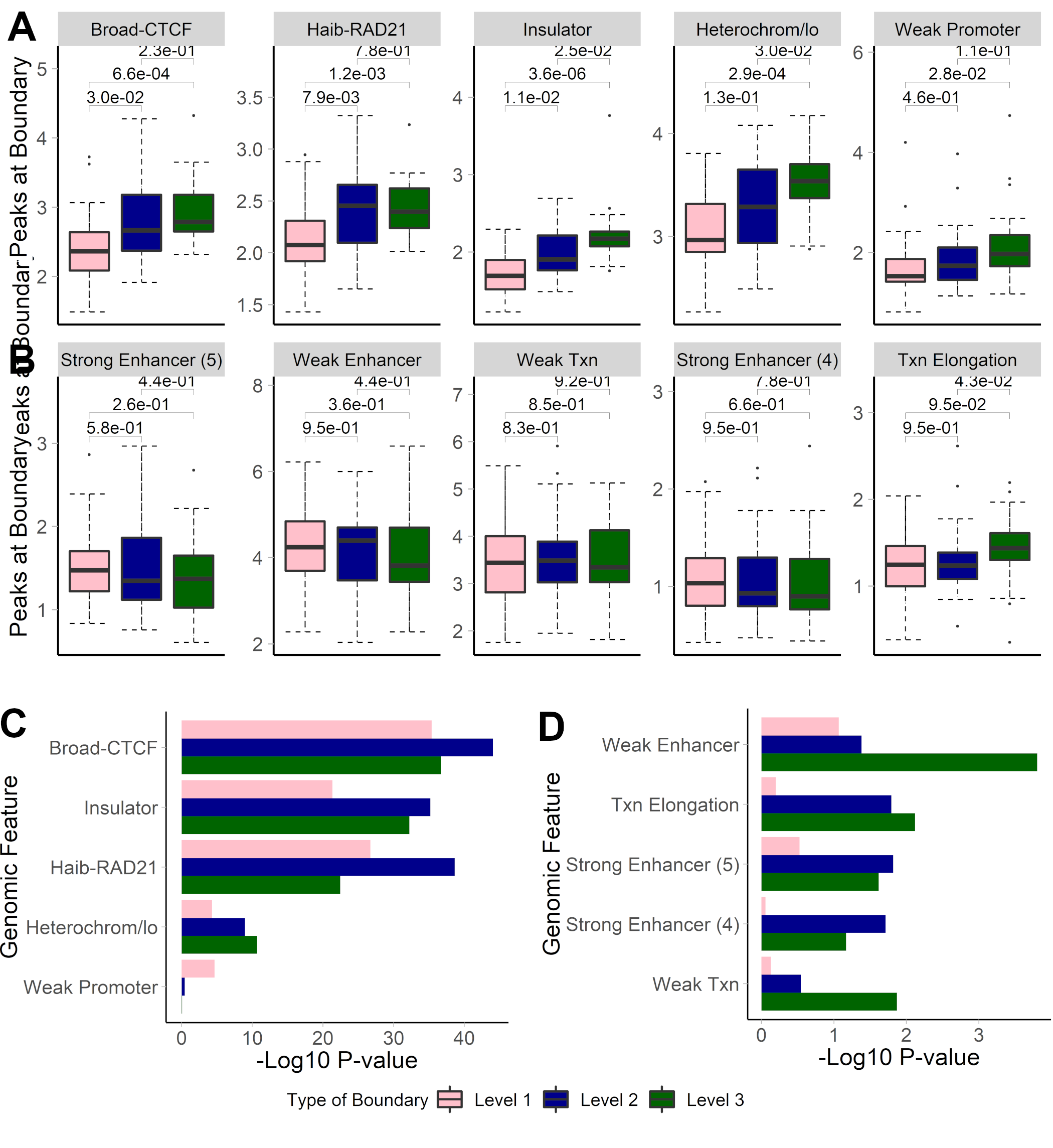 ]
---
## SpectralTAD is fast
A) Runtimes for various TAD callers at different chromosome sizes
B) Runtimes for various TAD callers across all chromosomes (25kb data)
.center[
]
---
## SpectralTAD is fast
A) Runtimes for various TAD callers at different chromosome sizes
B) Runtimes for various TAD callers across all chromosomes (25kb data)
.center[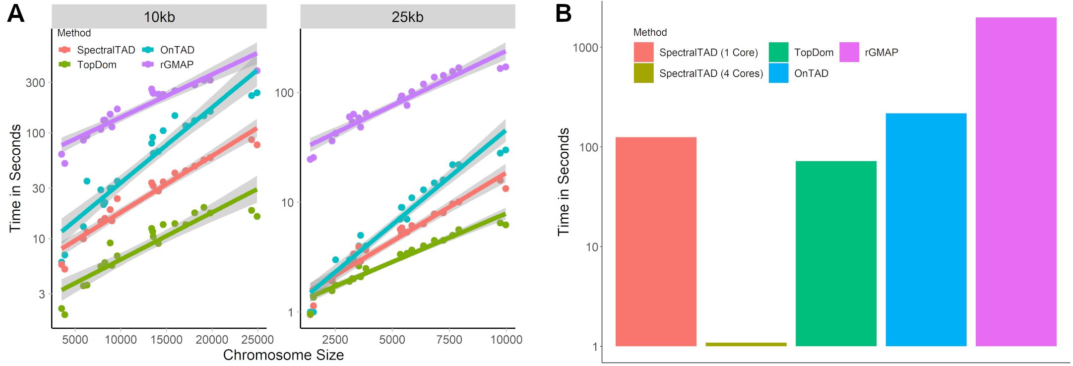 ]
---
## SpectralTAD Package
- **Input**: three types of contact matrices ( $n \times n$, sparse and $n \times (n+3)$) in text format, import from `.hic` and `.cool` files supported
- Two main functions: `SpectralTAD` and `SpectralTAD_Par` (parallelized)
- **Output**: A 3-column BED file for each hierarchy level
- Visualization options include output for `Juicebox`
]
---
## SpectralTAD Package
- **Input**: three types of contact matrices ( $n \times n$, sparse and $n \times (n+3)$) in text format, import from `.hic` and `.cool` files supported
- Two main functions: `SpectralTAD` and `SpectralTAD_Par` (parallelized)
- **Output**: A 3-column BED file for each hierarchy level
- Visualization options include output for `Juicebox`
.small[ https://bioconductor.org/packages/SpectralTAD/
Cresswell, Kellen G., John C. Stansfield, and Mikhail G. Dozmorov. “[SpectralTAD: An R Package for Defining a Hierarchy of Topologically Associated Domains Using Spectral Clustering](https://doi.org/10.1186/s12859-020-03652-w)” _BMC Bioinformatics_, July 20, 2020
]
---
class: center, middle
# TADcompare
Differential and time course analysis of TAD boundaries
---
## Comparing TADs (TADcompare)
.pull-left[
- Boundary score can be compared across conditions – differential boundary score
.center[]
]
.pull-right[ .center[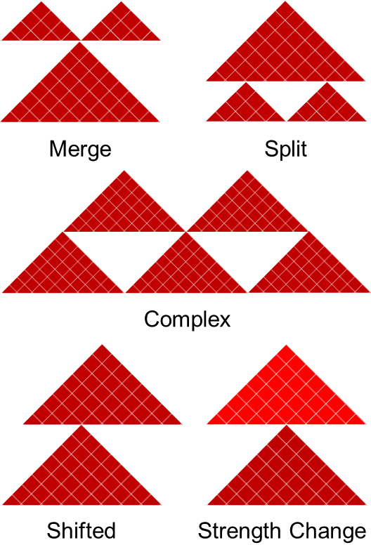 ] ]
.small[ Cresswell, Kellen G., and Mikhail G. Dozmorov. “[TADCompare: An R Package for Differential and Temporal Analysis of Topologically Associated Domains](https://doi.org/10.3389/fgene.2020.00158)” _Frontiers in Genetics_, March 10, 2020 ]
---
## Complex TAD boundary changes are frequent between biological replicates and cell/tissue types
.center[
] ]
.small[ Cresswell, Kellen G., and Mikhail G. Dozmorov. “[TADCompare: An R Package for Differential and Temporal Analysis of Topologically Associated Domains](https://doi.org/10.3389/fgene.2020.00158)” _Frontiers in Genetics_, March 10, 2020 ]
---
## Complex TAD boundary changes are frequent between biological replicates and cell/tissue types
.center[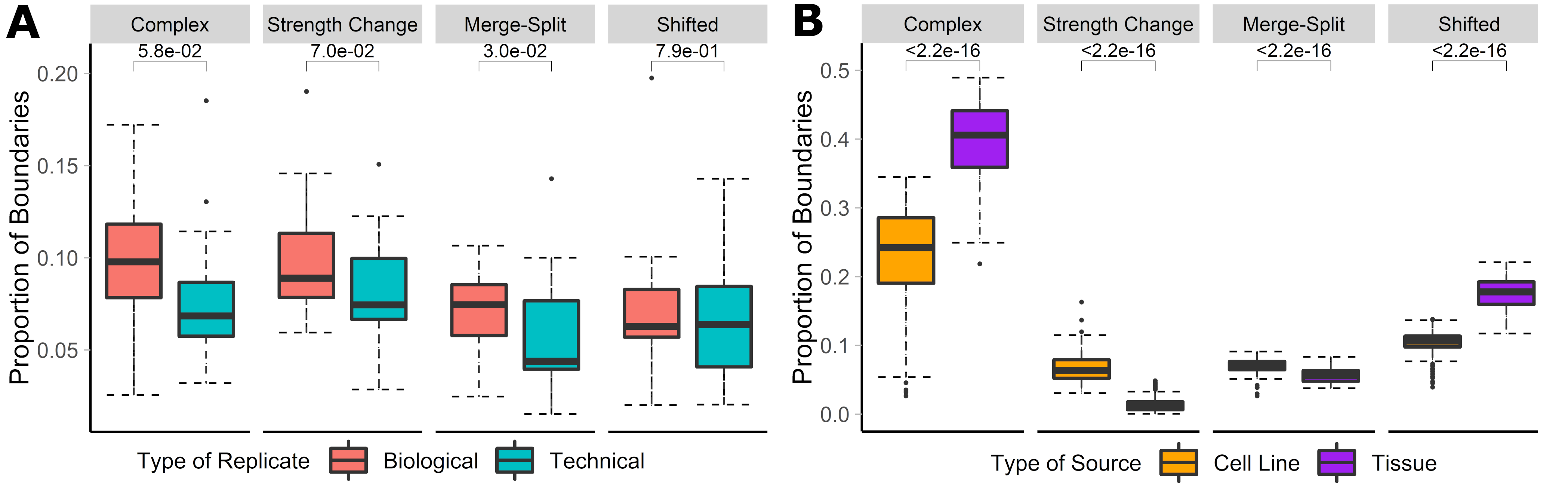 ]
---
## Distinct biology of differential TAD boundaries
- Non-differential boundaries are most enriched in CTCF and other boundary marks – conserved, biologically important
- Shifted boundaries are least enriched – shifts are likely due to noisy data
.center[
]
---
## Distinct biology of differential TAD boundaries
- Non-differential boundaries are most enriched in CTCF and other boundary marks – conserved, biologically important
- Shifted boundaries are least enriched – shifts are likely due to noisy data
.center[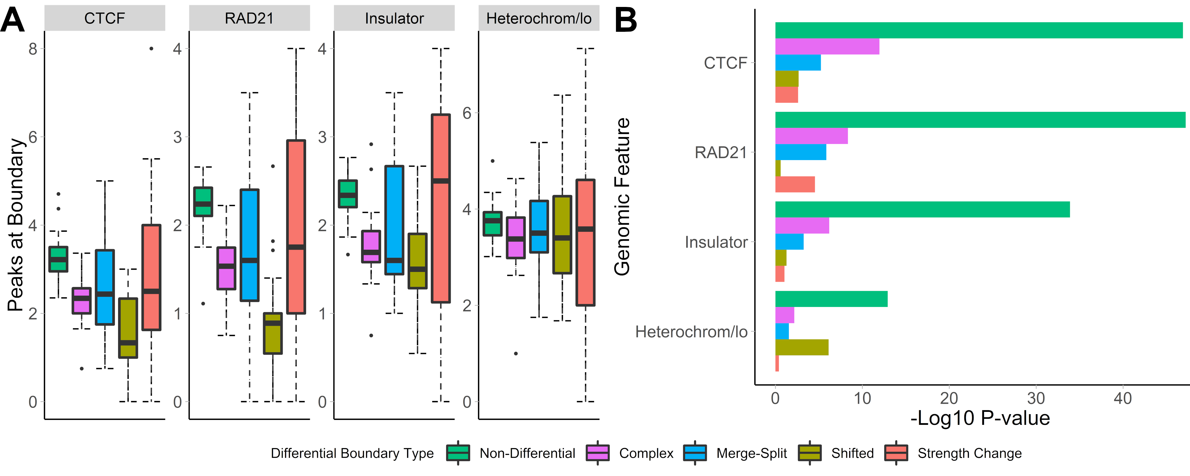 ]
---
## Dynamics of the 3D genome over time course
.pull-left[
- Boundary score allows investigating changes in TAD boundaries over time course
- Six patterns of boundary changes over time
]
.pull-right[ .center[
]
---
## Dynamics of the 3D genome over time course
.pull-left[
- Boundary score allows investigating changes in TAD boundaries over time course
- Six patterns of boundary changes over time
]
.pull-right[ .center[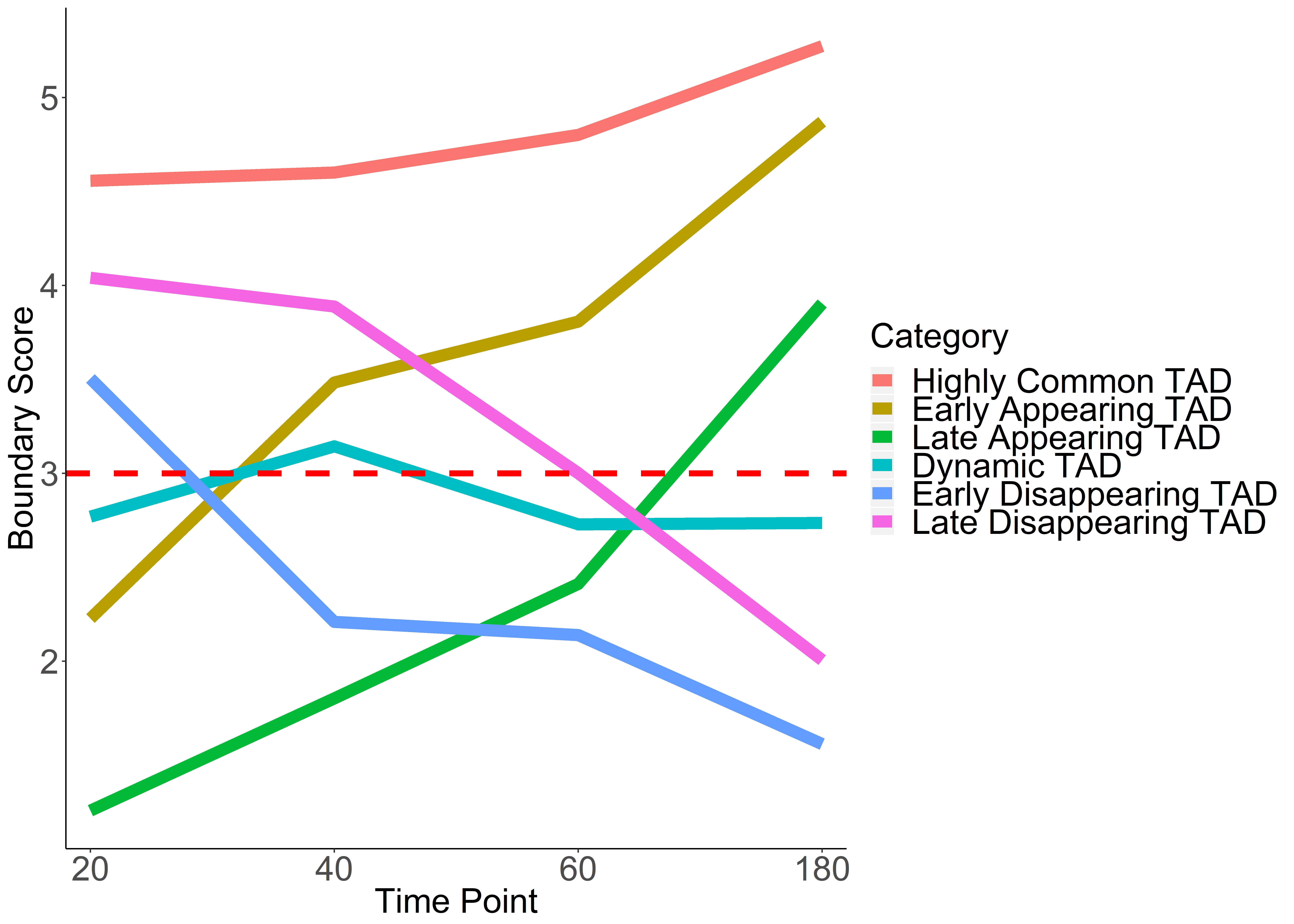 ] ]
---
## Distinct biology of different patterns of TAD boundary changes
- Auxin treatment experiment - eliminate TAD boundaries with auxin, wash auxin out, observe TAD boundaries recovery
- Early and Late appearing boundaries are most enriched in CTCF, RAD21
.center[
] ]
---
## Distinct biology of different patterns of TAD boundary changes
- Auxin treatment experiment - eliminate TAD boundaries with auxin, wash auxin out, observe TAD boundaries recovery
- Early and Late appearing boundaries are most enriched in CTCF, RAD21
.center[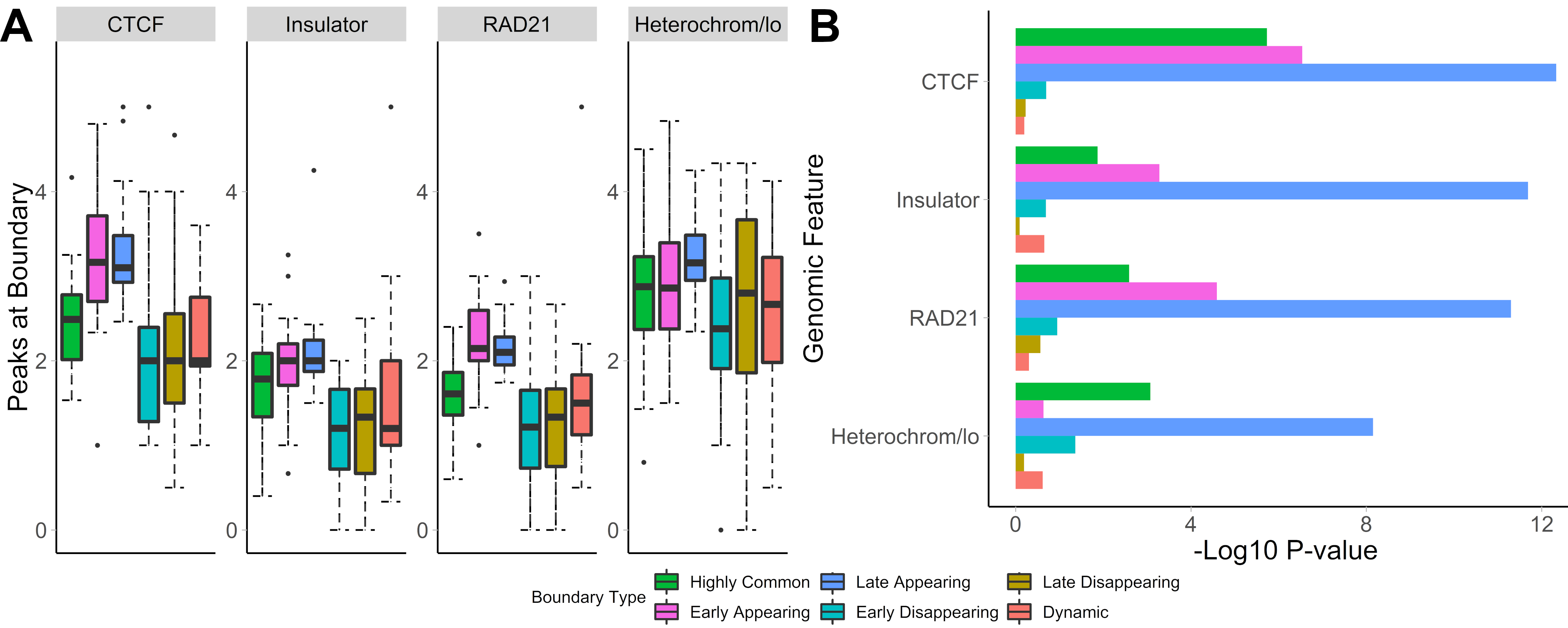 ]
---
## Time course Hi-C data analysis
- Part of the TADcompare package
- Requires three or more time points
- Can handle replicates at each time point
]
---
## Time course Hi-C data analysis
- Part of the TADcompare package
- Requires three or more time points
- Can handle replicates at each time point
.small[ https://bioconductor.org/packages/TADCompare/
Cresswell, Kellen G., and Mikhail G. Dozmorov. “[TADCompare: An R Package for Differential and Temporal Analysis of Topologically Associated Domains](https://doi.org/10.3389/fgene.2020.00158)” _Frontiers in Genetics_, March 10, 2020 ]
---
class: center, middle
# Understanding the biology of differential chromatin interactions
---
## 3D genome of cancer metastasis and drug resistance
- Patient Derived Xenograft (PDX) mouse models of breast cancer
- Progression of the primary tumor to metastatic and drug resistant states
.center[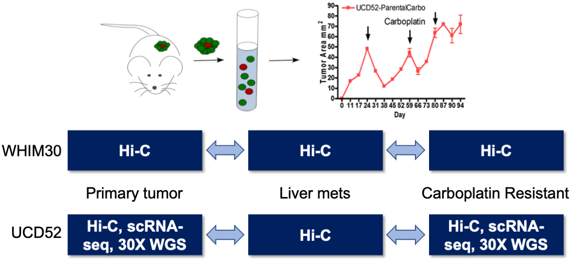 ]
---
## Analysis of PDX Hi-C data (PDX Hi-C)
.pull-left[
- Mouse reads minimally affect Hi-C data - direct alignment to the human genome works well
- Processing pipeline plays minimal role
- Technology is the most important for data quality
]
.pull-right[ .center[
]
---
## Analysis of PDX Hi-C data (PDX Hi-C)
.pull-left[
- Mouse reads minimally affect Hi-C data - direct alignment to the human genome works well
- Processing pipeline plays minimal role
- Technology is the most important for data quality
]
.pull-right[ .center[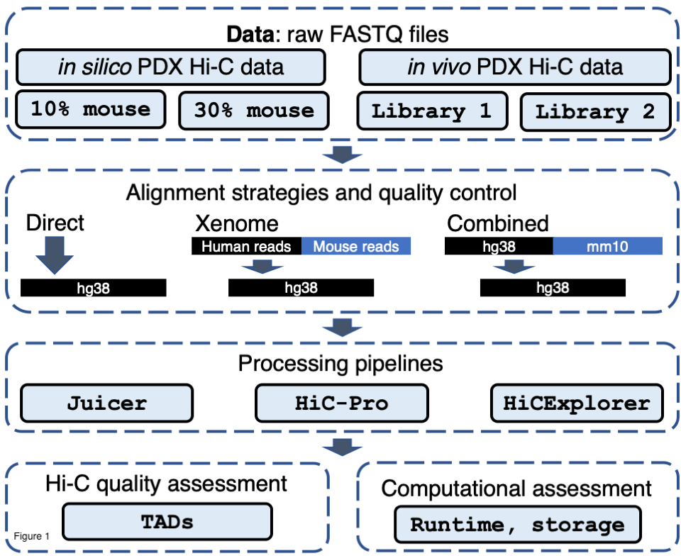 ] ]
.small[Dozmorov, Mikhail G, Katarzyna M Tyc, Nathan C Sheffield, David C Boyd, Amy L Olex, Jason Reed, and J Chuck Harrell. “[Chromatin Conformation Capture (Hi-C) Sequencing of Patient-Derived Xenografts: Analysis Guidelines](https://doi.org/10.1093/gigascience/giab022)” _GigaScience_ April 21, 2021]
---
## 3D genome of cancer metastasis and drug resistance
.center[
] ]
.small[Dozmorov, Mikhail G, Katarzyna M Tyc, Nathan C Sheffield, David C Boyd, Amy L Olex, Jason Reed, and J Chuck Harrell. “[Chromatin Conformation Capture (Hi-C) Sequencing of Patient-Derived Xenografts: Analysis Guidelines](https://doi.org/10.1093/gigascience/giab022)” _GigaScience_ April 21, 2021]
---
## 3D genome of cancer metastasis and drug resistance
.center[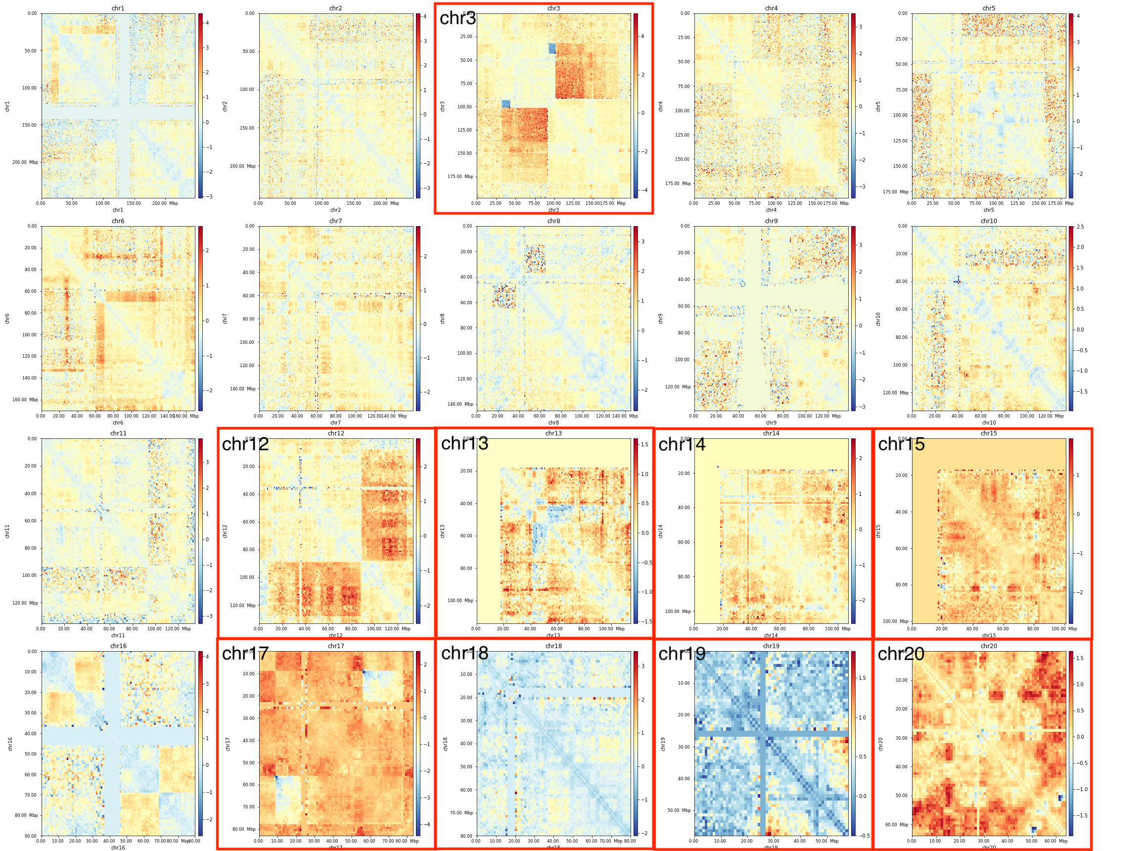 ]
---
## Summary
- **Distance-centric view** of Hi-C data is critical (`MD plot`)
- **Joint loess normalization** effectively removes between-dataset biases ([HiCcompare](https://bioconductor.org/packages/HiCcompare/))
- **Differential analysis considering distance** has optimal performance ([multiHiCcompare](https://bioconductor.org/packages/multiHiCcompare/))
- **Spectral clustering** robustly detects biologically relevant hierarchical TADs ([SpectralTAD](https://bioconductor.org/packages/SpectralTAD/))
- **Boundary score** enables differential and time course analysis of TAD boundaries ([TADcompare](https://bioconductor.org/packages/TADCompare/))
.small[https://github.com/mdozmorov/HiC_tools]
---
## Acknowledgements
.pull-left[ .center[
]
---
## Summary
- **Distance-centric view** of Hi-C data is critical (`MD plot`)
- **Joint loess normalization** effectively removes between-dataset biases ([HiCcompare](https://bioconductor.org/packages/HiCcompare/))
- **Differential analysis considering distance** has optimal performance ([multiHiCcompare](https://bioconductor.org/packages/multiHiCcompare/))
- **Spectral clustering** robustly detects biologically relevant hierarchical TADs ([SpectralTAD](https://bioconductor.org/packages/SpectralTAD/))
- **Boundary score** enables differential and time course analysis of TAD boundaries ([TADcompare](https://bioconductor.org/packages/TADCompare/))
.small[https://github.com/mdozmorov/HiC_tools]
---
## Acknowledgements
.pull-left[ .center[ ]
.small[https://dozmorovlab.github.io/]
]
.pull-rignt[ ### Collaborators
- J. Chuck Harrell (VCU, Pathology)
- Ay lab (La Jolla Institute for Immunology)
### Funding
- American Cancer Society
- PhRMA Foundation
- The George and Lavinia Blick Research Fund
.center[
]
.small[https://dozmorovlab.github.io/]
]
.pull-rignt[ ### Collaborators
- J. Chuck Harrell (VCU, Pathology)
- Ay lab (La Jolla Institute for Immunology)
### Funding
- American Cancer Society
- PhRMA Foundation
- The George and Lavinia Blick Research Fund
.center[ ]
]
---
class: center, middle
# Thank you
[bit.ly/3Dgenomics](https://mdozmorov.github.io/Talk_3Dgenome/)
]
]
---
class: center, middle
# Thank you
[bit.ly/3Dgenomics](https://mdozmorov.github.io/Talk_3Dgenome/)
Bioinformatics postdoc, research assistant positions available