# Welcome!  [](https://zenodo.org/badge/latestdoi/158620263)
[](https://github.com/mikejohnson51/climateR/actions/workflows/R-CMD-check.yaml)
[](#)
[](https://choosealicense.com/licenses/mit/)
[](https://www.repostatus.org/#active)
[](https://codecov.io/gh/mikejohnson51/climateR)
`climateR` simplifies the steps needed to get gridded geospatial data
into R. At its core, it provides three main things:
1. A catalog of 112398 geospatial climate, land cover, and soils
resources from 3477 collections. See (`climateR::catalog`)
This catalog is an [evolving, federated collection of
datasets](https://github.com/mikejohnson51/climateR-catalogs) that can
be accessed by the data access utilities. This resource is rebuilt
automatically on a monthly cycle to ensure the data provided is
accurate, while continuously growing based on user requests.
2. A general [toolkit for accessing remote and local gridded
data](https://mikejohnson51.github.io/climateR/reference/index.html#data-access)
files bounded by space, time, and variable constraints (`dap`,
`dap_crop`, `read_dap_file`)
3. A set of
[shortcuts](https://mikejohnson51.github.io/climateR/reference/index.html#shortcuts)
that implement these methods for a core set of selected catalog
elements
> :warning: **Python Users**: Data catalog access is available through
> the USGS [`gdptools`](https://gdptools.readthedocs.io/en/latest/)
> package. Directly analogous climateR functionality can be found in
> [`climatePy`](https://github.com/LynkerIntel/climatePy)
# Installation
``` r
remotes::install_github("mikejohnson51/AOI") # suggested!
remotes::install_github("mikejohnson51/climateR")
```
``` r
library(climateR)
```
# Basic Usage
The examples used here call upon the following shortcuts:
- `getGridMET` (OPeNDAP server, historic data)
- `getMODIS` (Authenticated OPeNDAP server)
- `getMACA` (OPeNDAP server, projection data)
- `getNLCD` (COG)
- `get3DEP` (VRT)
- `getCHIRPS` (erddap)
With the aim of highlighting the convenience of a consistent access
patterns for a variety of data stores.
### Defining Areas/Points of Interest
`climateR` is designed with the same concepts as `AOI`. Namely, that all
spatial data aggregation questions must start with an extent/area of
interest.
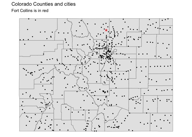
Before extracting any data, you must provide an. For the examples here,
we will use the state of Colorado (polygons), and all of its cities
(points).
``` r
colorado = aoi_get(state = "CO", county = "all")
cities = readRDS(system.file("co/cities_colorado.rds", package = "climateR"))
```
[](https://zenodo.org/badge/latestdoi/158620263)
[](https://github.com/mikejohnson51/climateR/actions/workflows/R-CMD-check.yaml)
[](#)
[](https://choosealicense.com/licenses/mit/)
[](https://www.repostatus.org/#active)
[](https://codecov.io/gh/mikejohnson51/climateR)
`climateR` simplifies the steps needed to get gridded geospatial data
into R. At its core, it provides three main things:
1. A catalog of 112398 geospatial climate, land cover, and soils
resources from 3477 collections. See (`climateR::catalog`)
This catalog is an [evolving, federated collection of
datasets](https://github.com/mikejohnson51/climateR-catalogs) that can
be accessed by the data access utilities. This resource is rebuilt
automatically on a monthly cycle to ensure the data provided is
accurate, while continuously growing based on user requests.
2. A general [toolkit for accessing remote and local gridded
data](https://mikejohnson51.github.io/climateR/reference/index.html#data-access)
files bounded by space, time, and variable constraints (`dap`,
`dap_crop`, `read_dap_file`)
3. A set of
[shortcuts](https://mikejohnson51.github.io/climateR/reference/index.html#shortcuts)
that implement these methods for a core set of selected catalog
elements
> :warning: **Python Users**: Data catalog access is available through
> the USGS [`gdptools`](https://gdptools.readthedocs.io/en/latest/)
> package. Directly analogous climateR functionality can be found in
> [`climatePy`](https://github.com/LynkerIntel/climatePy)
# Installation
``` r
remotes::install_github("mikejohnson51/AOI") # suggested!
remotes::install_github("mikejohnson51/climateR")
```
``` r
library(climateR)
```
# Basic Usage
The examples used here call upon the following shortcuts:
- `getGridMET` (OPeNDAP server, historic data)
- `getMODIS` (Authenticated OPeNDAP server)
- `getMACA` (OPeNDAP server, projection data)
- `getNLCD` (COG)
- `get3DEP` (VRT)
- `getCHIRPS` (erddap)
With the aim of highlighting the convenience of a consistent access
patterns for a variety of data stores.
### Defining Areas/Points of Interest
`climateR` is designed with the same concepts as `AOI`. Namely, that all
spatial data aggregation questions must start with an extent/area of
interest.
Before extracting any data, you must provide an. For the examples here,
we will use the state of Colorado (polygons), and all of its cities
(points).
``` r
colorado = aoi_get(state = "CO", county = "all")
cities = readRDS(system.file("co/cities_colorado.rds", package = "climateR"))
```
 ## Extent extraction
The default behavior of `climateR` is to request data for the extent of
the AOI passed regardless of whether it is `POINT` or `POLYGON` data.
The *exception* to the default behavior is if the the AOI is a single
point. To illustrate:
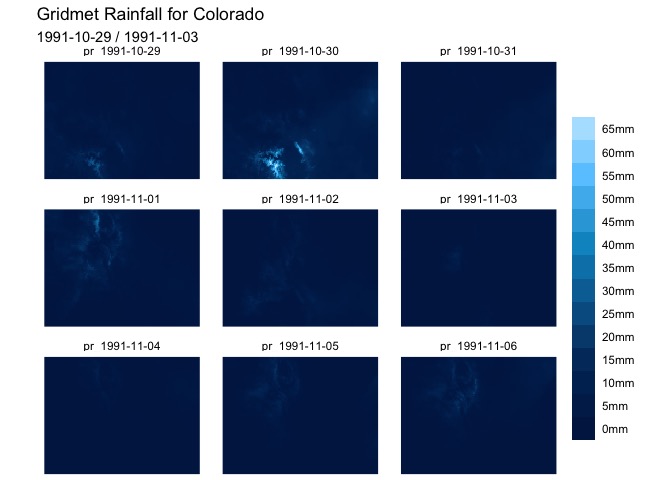
#### POLYGON(s) act as a single extent
``` r
# Request Data for Colorado (POLYGON(s))
system.time({
gridmet_pr = getGridMET(AOI = colorado,
varname = "pr",
startDate = "1991-10-29",
endDate = "1991-11-06")
})
#> user system elapsed
#> 0.195 0.021 1.266
```
## Extent extraction
The default behavior of `climateR` is to request data for the extent of
the AOI passed regardless of whether it is `POINT` or `POLYGON` data.
The *exception* to the default behavior is if the the AOI is a single
point. To illustrate:
#### POLYGON(s) act as a single extent
``` r
# Request Data for Colorado (POLYGON(s))
system.time({
gridmet_pr = getGridMET(AOI = colorado,
varname = "pr",
startDate = "1991-10-29",
endDate = "1991-11-06")
})
#> user system elapsed
#> 0.195 0.021 1.266
```
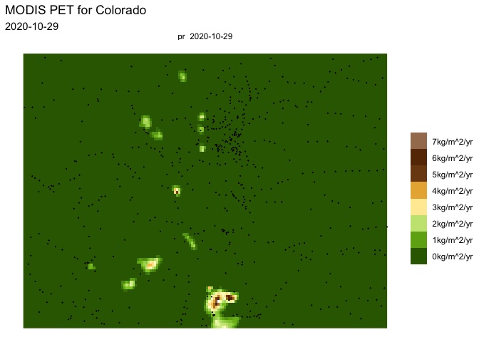
 #### POINTS(s) act as a single extent
``` r
# Request data using cities (POINTs)
pr = getGridMET(
AOI = cities,
varname = "pr",
startDate = "2020-10-29")
```
#### POINTS(s) act as a single extent
``` r
# Request data using cities (POINTs)
pr = getGridMET(
AOI = cities,
varname = "pr",
startDate = "2020-10-29")
```
 #### Single POINT(s) act as an extent
However since the extent of a POINT means `{xmax = xmin}` and
`{ymax = ymin}`, climateR will return a time series of the intersecting
cell, opposed to a one cell `SpatRaster`.
``` r
# Request data for a single city
system.time({
future_city = getMACA(AOI = cities[1,],
varname = "tasmax",
startDate = "2050-10-29",
endDate = "2050-11-06")
})
#> user system elapsed
#> 0.203 0.005 0.547
```
``` r
future_city
#> date tasmax_CCSM4_r6i1p1_rcp45
#> 1 2050-10-29 295.7503
#> 2 2050-10-30 292.0839
#> 3 2050-10-31 289.6805
#> 4 2050-11-01 287.1293
#> 5 2050-11-02 290.7788
#> 6 2050-11-03 287.1146
#> 7 2050-11-04 290.1259
#> 8 2050-11-05 291.0247
#> 9 2050-11-06 291.6172
```
#### Dynamic AOIs, tidyverse piping
All `climateR` functions treat the extent of the AOI and the default
extraction area. This allows multiple climateR shortcuts to be chained
together using either the base R or dplyr piping syntax.
``` r
pipes = aoi_ext("Fort Collins", wh = c(10, 20), units = "km", bbox = TRUE)|>
getNLCD() |>
getTerraClimNormals(varname = c("tmax", "ppt"))
lapply(pipes, dim)
#> $`2019 Land Cover L48`
#> [1] 1402 786 1
#>
#> $tmax
#> [1] 10 8 12
#>
#> $ppt
#> [1] 10 8 12
```
### Extract timeseries from exisitng objects:
Using `extract_sites`, you can pass an existing data object. If no
identified column is provided to name the extracted timeseries, the
first, fully unique column in the data.frame is used:
``` r
gridmet_pts = extract_sites(gridmet_pr, pts = cities)
names(gridmet_pts)[1:5]
#> [1] "date" "177" "283" "527" "117"
gridmet_pts = extract_sites(gridmet_pr, pts = cities, ID = 'NAME')
names(gridmet_pts)[1:5]
#> [1] "date" "ADAMSCITY" "AGATE" "AGUILAR" "AKRON"
```
# Unit Based Extraction
While the default behavior is to extract data by **extent**, there are
cases when the input AOI is a set of discrete units that you *want* to
act as discrete units.
- A set of `POINT`s from which to extract time series
- A set of `POLYGON`s that data should be summarized to (mean, max, min,
etc.) (**WIP**)
In `climateR`, populating the `ID` parameter of any shortcut (or `dap`)
function, triggers data to be extracted by unit.
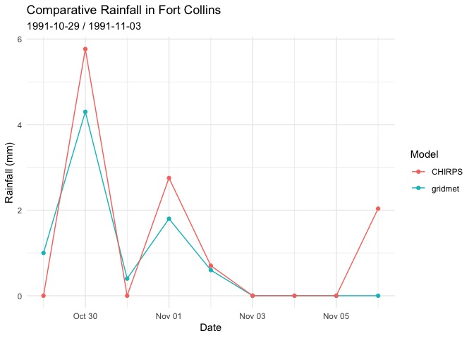
### Extact timeseries for POINTs
In the `cities` object, the individual `POINT`s are uniquely identified
by a `NAME` column. Tellings a climateR function, that `ID = "NAME"`
triggers it to return the summary:
``` r
chirps_pts = getCHIRPS(AOI = cities,
varname = "precip",
startDate = "1991-10-29",
endDate = "1991-11-06",
ID = "NAME")
dim(chirps_pts)
#> [1] 9 584
names(chirps_pts)[1:5]
#> [1] "date" "ADAMSCITY" "AGATE" "AGUILAR" "AKRON"
```
#### Single POINT(s) act as an extent
However since the extent of a POINT means `{xmax = xmin}` and
`{ymax = ymin}`, climateR will return a time series of the intersecting
cell, opposed to a one cell `SpatRaster`.
``` r
# Request data for a single city
system.time({
future_city = getMACA(AOI = cities[1,],
varname = "tasmax",
startDate = "2050-10-29",
endDate = "2050-11-06")
})
#> user system elapsed
#> 0.203 0.005 0.547
```
``` r
future_city
#> date tasmax_CCSM4_r6i1p1_rcp45
#> 1 2050-10-29 295.7503
#> 2 2050-10-30 292.0839
#> 3 2050-10-31 289.6805
#> 4 2050-11-01 287.1293
#> 5 2050-11-02 290.7788
#> 6 2050-11-03 287.1146
#> 7 2050-11-04 290.1259
#> 8 2050-11-05 291.0247
#> 9 2050-11-06 291.6172
```
#### Dynamic AOIs, tidyverse piping
All `climateR` functions treat the extent of the AOI and the default
extraction area. This allows multiple climateR shortcuts to be chained
together using either the base R or dplyr piping syntax.
``` r
pipes = aoi_ext("Fort Collins", wh = c(10, 20), units = "km", bbox = TRUE)|>
getNLCD() |>
getTerraClimNormals(varname = c("tmax", "ppt"))
lapply(pipes, dim)
#> $`2019 Land Cover L48`
#> [1] 1402 786 1
#>
#> $tmax
#> [1] 10 8 12
#>
#> $ppt
#> [1] 10 8 12
```
### Extract timeseries from exisitng objects:
Using `extract_sites`, you can pass an existing data object. If no
identified column is provided to name the extracted timeseries, the
first, fully unique column in the data.frame is used:
``` r
gridmet_pts = extract_sites(gridmet_pr, pts = cities)
names(gridmet_pts)[1:5]
#> [1] "date" "177" "283" "527" "117"
gridmet_pts = extract_sites(gridmet_pr, pts = cities, ID = 'NAME')
names(gridmet_pts)[1:5]
#> [1] "date" "ADAMSCITY" "AGATE" "AGUILAR" "AKRON"
```
# Unit Based Extraction
While the default behavior is to extract data by **extent**, there are
cases when the input AOI is a set of discrete units that you *want* to
act as discrete units.
- A set of `POINT`s from which to extract time series
- A set of `POLYGON`s that data should be summarized to (mean, max, min,
etc.) (**WIP**)
In `climateR`, populating the `ID` parameter of any shortcut (or `dap`)
function, triggers data to be extracted by unit.
### Extact timeseries for POINTs
In the `cities` object, the individual `POINT`s are uniquely identified
by a `NAME` column. Tellings a climateR function, that `ID = "NAME"`
triggers it to return the summary:
``` r
chirps_pts = getCHIRPS(AOI = cities,
varname = "precip",
startDate = "1991-10-29",
endDate = "1991-11-06",
ID = "NAME")
dim(chirps_pts)
#> [1] 9 584
names(chirps_pts)[1:5]
#> [1] "date" "ADAMSCITY" "AGATE" "AGUILAR" "AKRON"
```
 ### Integration with `zonal`
While climateR does not yet provide areal summaries, our intention is to
integrate the functionality from `zonal`. Until then, `climateR` outputs
can be piped directly into `execute_zonal`. The zonal package also
requires a uniquely identifying column name, and a function to summarize
data with.
``` r
library(zonal)
system.time({
chirps = getCHIRPS(AOI = colorado,
varname = "precip",
startDate = "1991-10-29",
endDate = "1991-11-06") %>%
execute_zonal(geom = colorado,
fun = "max",
ID = "fip_code")
})
#> user system elapsed
#> 0.174 0.012 1.245
```
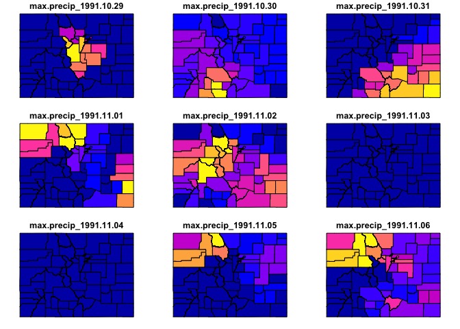
### Integration with `zonal`
While climateR does not yet provide areal summaries, our intention is to
integrate the functionality from `zonal`. Until then, `climateR` outputs
can be piped directly into `execute_zonal`. The zonal package also
requires a uniquely identifying column name, and a function to summarize
data with.
``` r
library(zonal)
system.time({
chirps = getCHIRPS(AOI = colorado,
varname = "precip",
startDate = "1991-10-29",
endDate = "1991-11-06") %>%
execute_zonal(geom = colorado,
fun = "max",
ID = "fip_code")
})
#> user system elapsed
#> 0.174 0.012 1.245
```
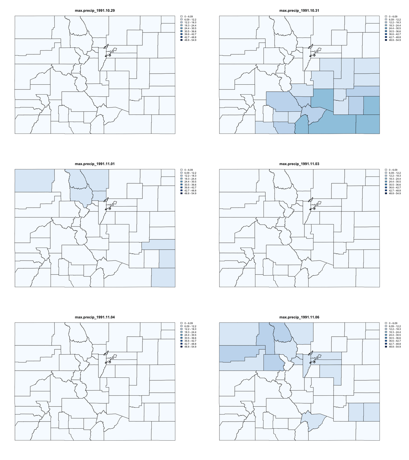
 ## Basic Animation
### Gridded
``` r
animation(gridmet_pr$precipitation_amount, AOI = AOI, outfile = "man/figures/rast_gif.gif")
```
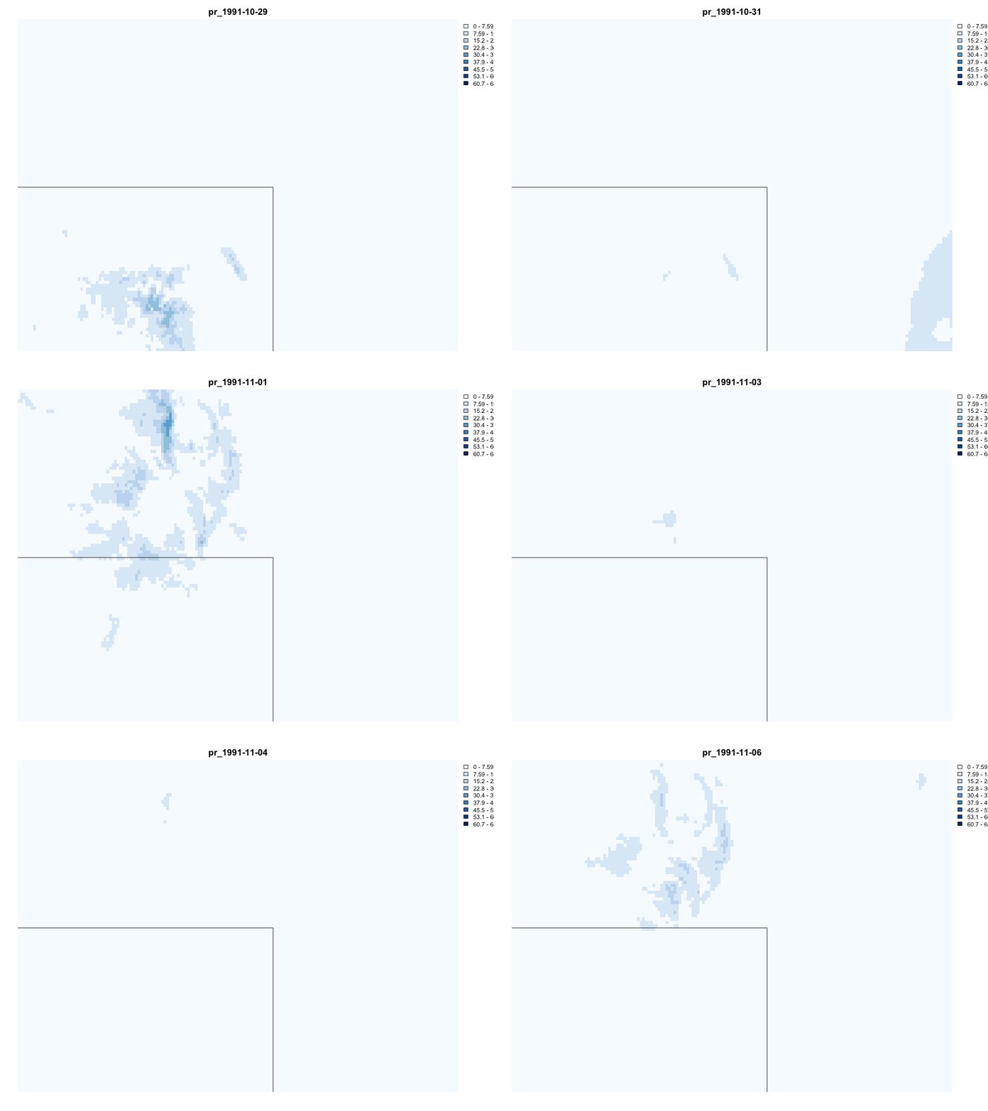
## Basic Animation
### Gridded
``` r
animation(gridmet_pr$precipitation_amount, AOI = AOI, outfile = "man/figures/rast_gif.gif")
```
 ### Polygon
``` r
animation(max, feild_pattern = "precip_", outfile = "man/figures/vect_gif.gif")
```
### Polygon
``` r
animation(max, feild_pattern = "precip_", outfile = "man/figures/vect_gif.gif")
```