---
title: "R Workshop / Duke MEM"
author: "Mine Cetinkaya-Rundel"
date: "October 14, 2015"
output: ioslides_presentation
---

```{r setup, echo=FALSE}
knitr::opts_chunk$set(echo = TRUE)
```

# Intro

## Outline

- Introduction to R and RStudio
- Reproducible data analysis with R Markdown
- Loading data
- Data visualization
- Data wrangling
- Basic R syntax
- What next?
- Hands on exercises

## Materials

- All source code at https://github.com/mine-cetinkaya-rundel/rworkshop-mem

- Slides at http://rpubs.com/minebocek/117428

# Introduction to R and RStudio

## What is R and RStudio

- **R\:** Statistical programming language

- **RStudio\:** 
    - Inregtrated development environment for R
    - Powerful and productive user interface for R

- Both are free and open-source

## Getting started

- Traditionally you would install R and RStudio on your computer

- We will skip over that step for now for efficiency and use the RStudio server at

https://vm-manage.oit.duke.edu/containers

(Log in with your Duke Net ID and password)

- Local installation instructions will be provided at the end of the workshop

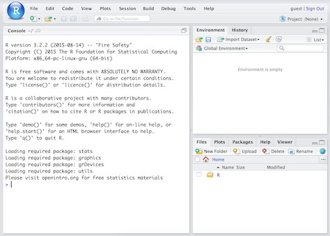
## Anatomy of RStudio

<div class="columns-2">
- Left: Console
    - Text on top at launch: version of R that you’re running
    - Below that is the prompt
- Upper right: Workspace and command history
- Lower right: Plots, access to files, help, packages, data viewer

![R Splash Screen](img/RStudioSplash.png)
</div>

## What version am I using?

- The version of R is text that pops up in the Console when you start RStudio

- To find out the version of RStudio go to Help $\rightarrow$ About RStudio

- It's good practice to keep both R and RStudio up to date

## R packages {.smaller}

- Packages are the fundamental units of reproducible R code. They include reusable R
functions, the documentation that describes how to use them, and (often) sample data.
(From: http://r-pkgs.had.co.nz)

- We will use the `ggplot2` package for plots and `dplyr` for data wrangling in this
workshop

- Install these packages by running the following in the Console:
```{r install-packages, eval=FALSE}
install.packages("ggplot2")
install.packages("dplyr")
```

- Then, load the packages by running the following:
```{r load-packages, message=FALSE}
library(ggplot2)
library(dplyr)
```
    
- This is just one way of installing a package, there is also a GUI approach in 
the Packages pane in RStudio

# Reproducible data analysis with R Markdown

## What is R Markdown?

- R Markdown is an authoring format that enables easy creation of dynamic documents, 
presentations, and reports from R. 

- It combines the core syntax of markdown (an easy-to-write plain text format) with 
embedded R code chunks that are run so their output can be included in the final document.

- R Markdown documents are fully **reproducible** (they can be automatically regenerated 
whenever underlying R code or data changes).

Source: http://rmarkdown.rstudio.com/

## Your turn!

Create your first R Markdown document, knit it, and examine the source code 
and the output.

1. File $\rightarrow$ R Markdown...

2. Enter a title (e.g. "My first R Markdown document") and author info

3. Choose Document as file type, and HTML as the output

4. Hit OK

5. Click Knit HTML in the new document, which will prompt you to save your document
    - Naming tip: Do not use spaces
    - Viewing tip: Click on the down arrow next to Knit HTML and select View in Pane
    
## Markdown basics {.smaller}

- Markdown is a simple formatting language designed to make authoring content easy for 
everyone. 

- Rather than writing complex markup code (e.g. HTML or LaTeX), Markdown enables the use 
of a syntax much more like plain-text email. 

![Markdown overview](img/markdownOverview.png)

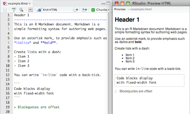
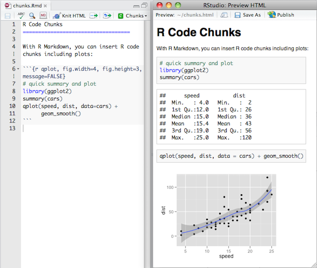
## R Code Chunks {.smaller}

Within an R Markdown file, R Code Chunks can be embedded using the native Markdown syntax 
for fenced code regions.

![Code chunks](img/markdownChunk.png)

## Your turn!

How many code chunks are in your R Markdown document?

What does each code chunk do? You may not understand the R syntax yet,
but you should be able to compare the source file and the output to answer
this question.

## Inline R Code

You can also evaluate R expressions inline by enclosing the expression within a single 
back-tick qualified with ‘r’. For example, the following code:

![Inline code](img/markdownInline.png)

Results in this output: "I counted `r 1 + 1` red trucks on the highway."

## Your turn!

Suppose Sammy works on average 8.37 hours per day, 5 days
per week. How many hours does Sammy work on average per week?

Add a sentence to your document that includes simple inline R code that answers
this question, along the lines of...

"Sammy works 8.37 * 5 hours per week, on average."

## Workspaces

R Markdown workspace and Console workspace are independent of each other

- If you define a variable in your Console and it shows up in the Environment
tab, it is not going to be automatically included in your R Markdown document

- If you define a variable in your R Markdown document, it won't automatically
be available in your Console
    
[ Demo ]

**Tip\:** Use the *Run all previous chunks* in the source file and *Run current chunk
code* functionality in the buttons in each code chunk to help manage workspaces.

## Workspaces and reproducibilty

- The fact that the two workspaces do not automatically have access to the same variables
might / will be frustrating at first.

- But this is not a bug, in fact, it's a functionality that helps reproducibility, as it
ensures that all variables, functions, etc. that are being used in the R Markdown 
document are explicitly defined or loaded.

## Your turn! {.smaller}

1. Define `x = 2` in the Console. Then, in your Console run `x * 3`. Does your code 
run as expected?

2. Now, insert a new code chunk in your R Markdown document and in this chunk type
`x * 3` only. Knit your document. Does the document compile, or do you get an error?
If you get an error, what does the error say, and how can you fix it? Implement the fix 
and Knit your document. Make sure you are able to compile without errors before you 
move on.

**Tip\:** Insert a new code chunk bu clicking Chunks $\rightarrow$ Insert Chunk.

3. Next insert another code chunk in your R Markdown document and define `y = 4` and
calculate `y + 5`. Knit your document. Does everything work as expected?

4. Now run `y + 5` in your Console. Does your code run as expected or do you get an error?
If you get an error, what does the error say, and how can you fix it? Implement the fix.

## Code chunk options

- You can hide the code, hide the result, hide warnings, messages, etc.

- Refer to the handy R Markdown 
[cheatsheet](https://www.rstudio.com/wp-content/uploads/2015/02/rmarkdown-cheatsheet.pdf)

- Another good reference: http://rmarkdown.rstudio.com/authoring_rcodechunks.html

# Loading data

## NC DOT Fatal Crashes in North Carolina {.smaller}

```{r load-data}
bike <- read.csv("https://stat.duke.edu/~mc301/data/nc_bike_crash.csv", 
                 sep = ";", stringsAsFactors = FALSE, na.strings = c("NA", "", ".")) %>%
  tbl_df()
```

View the names of variables via
```{r}
names(bike)
```

and see detailed descriptions at https://stat.duke.edu/~mc301/data/nc_bike_crash.html.

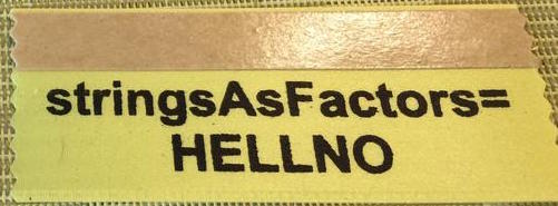
## Aside: Strings (characters) vs factors

- By default R will convert character vectors into factors when they are
included in a data frame.

- Sometimes this is useful, sometimes it isn't – either way it is 
important to know what type/class you are working with.

- This behavior can be changed using the `stringsAsFactors = FALSE` 
when loading a data drame.

![stringsAsFactorsHELLNO](img/stringsAsFactors.jpg)

## Viewing your data {.smaller}

- In the Environment, click on the name of the data frame to view
it in the data viewer

- Use the `str()` function to compactly display the internal **str**ucture 
of an R object

```{r}
str(bike)
```

# Data visualization

## Data visualization in R

- Using base R functions

- Using the `ggplot2` package $\leftarrow$ our focus today

- Using a variety of other packages like `lattice`, `ggvis`, etc.

## The Grammar of Graphics

- Visualisation concept created by Wilkinson (1999)
    - to define the basic elements of a statistical graphic 

- Adapted for R by Wickham (2009) who created the `ggplot2` package
    - consistent and compact syntax to describe statistical graphics
    - highly modular as it breaks up graphs into semantic components 

- Is not a guide which graph to choose and how to convey information best!

Source: https://rpubs.com/timwinke/ggplot2workshop

## The Grammar of Graphics - Terminology

A statistical graphic is a...

- mapping of **data**
- to **aesthetic attributes** (color, size, xy-position)
- using **geometric objects** (points, lines, bars)
- with data being **statistically transformed** (summarised, log-transformed)
- and mapped onto a specific **facet** and **coordinate system**
    
## Biker age vs. crash hour {.smaller}

```{r echo=FALSE, fig.height=3, fig.width=5, warning=FALSE}
ggplot(data = bike, aes(x = Crash_Hour, y = Bike_Age)) +
  geom_point()
```

- Which data is used as an input?
- What geometric objects are chosen for visualization?
- What variables are mapped onto which attributes?
- What type of scales are used to map data to aesthetics?
- Are the variables statistically transformed before plotting?

## Biker age vs. crash hour - code

```{r fig.height=3, fig.width=5}
ggplot(data = bike, aes(x = Crash_Hour, y = Bike_Age)) +
  geom_point()
```

## Altering features {.smaller}

```{r echo=FALSE, fig.height=3, fig.width=5, warning=FALSE}
ggplot(data = bike, aes(x = Crash_Hour, y = Bike_Age)) +
  geom_point(alpha = 0.5, color = "blue")
```

- How did the plot change?
- Are these changes based on data (i.e. can be mapped to variables in the dataset) or
changes in preferences for geometric objects?

## Altering features - code

```{r fig.height=3, fig.width=5}
ggplot(data = bike, aes(x = Crash_Hour, y = Bike_Age)) +
  geom_point(alpha = 0.5, color = "blue")
```

## More alterations {.smaller}

```{r echo=FALSE, fig.height=3, fig.width=8, warning=FALSE}
ggplot(data = bike, aes(x = Crash_Hour, y = Bike_Age, color = AmbulanceR)) +
  geom_point(alpha = 0.5) +
  facet_grid(. ~ Bike_Sex)
```

- How did the plot change?
- Are these changes based on data (i.e. can be mapped to variables in the dataset) or
changes in preferences for geometric objects?

## More alterations - code {.smaller}

```{r fig.height=3, fig.width=8, warning=FALSE}
ggplot(data = bike, aes(x = Crash_Hour, y = Bike_Age, color = AmbulanceR)) +
  geom_point(alpha = 0.5) +
  facet_grid(. ~ Bike_Sex)
```

## Anatomy of ggplots

```
ggplot(data = [dataframe], aes(x = [var_x], y = [var_y], 
       color = [var_for_color], fill = [var_for_fill], 
       shape = [var_for_shape])) +
    geom_[some_geom] +
    ... # other options
```

## Histograms

```{r fig.height=3, fig.width=7, warning=FALSE}
ggplot(data = bike, aes(x = Bike_Age)) +
  geom_histogram(binwidth = 5)
```

## Boxplots

```{r fig.height=3, fig.width=8, warning=FALSE}
ggplot(data = bike, aes(y = Bike_Age, x = Bike_Sex)) +
  geom_boxplot()
```

## Barplots

```{r fig.height=3, fig.width=8, warning=FALSE}
ggplot(data = bike, aes(x = Bike_Injur)) +
  geom_bar()
```

## Segmented barplots

```{r fig.height=3, fig.width=9, warning=FALSE}
ggplot(data = bike, aes(x = Crash_Loc, fill = Bike_Injur)) +
  geom_bar()
```

## Segmented barplots - proportions

```{r fig.height=3, fig.width=9, warning=FALSE}
ggplot(data = bike, aes(x = Crash_Loc, fill = Bike_Injur)) +
  geom_bar(position="fill")
```

## More `ggplot2` resources

- Visit http://docs.ggplot2.org/current/ for documentation on the current version
of the `ggplot2` package. It's full of examples!

- Refer to the `ggplot2` 
[cheatsheet](https://www.rstudio.com/wp-content/uploads/2015/08/ggplot2-cheatsheet.pdf).

# Data wrangling

## Data wrangling in R

- Using base R functions

- Using the `dplyr` package $\leftarrow$ our focus today

- Using a variety of other packages like `plyr`, `tidyr`, `lubridate`, etc.

## Data wrangling with `dplyr`

The `dplyr` package is based on the concepts of functions as verbs that 
manipulate data frames:

- `filter()`: pick rows matching criteria
- `select()`: pick columns by name 
- `rename()`: rename specific columns
- `arrange()`: reorder rows 
- `mutate()`: add new variables
- `transmute()`: create new data frame with variables
- `sample_n()` / `sample_frac()`: randomly sample rows
- `summarise()`: reduce variables to values

## `dplyr` rules

- First argument is a data frame
- Subsequent arguments say what to do with data frame
- Always return a data frame 
- Avoid modify in place

## Filter rows with `filter()`

- Select a subset of rows in a data frame.
- Easily filter for many conditions at once.

## `filter()` {.smaller}

for crashes in Durham County

```{r}
bike %>%
  filter(County == "Durham")
```

## `filter()` {.smaller}

for crashes in Durham County where biker was < 10 yrs old

```{r}
bike %>%
  filter(County == "Durham", Bike_Age < 10)
```

## Commonly used logical operators in R {.smaller}

operator    | definition
------------|--------------------------
`<`         | less than
`<=`        |	less than or equal to
`>`         | greater than
`>=`        |	greater than or equal to
`==`        |	exactly equal to
`!=`        |	not equal to
`x | y`     | `x` OR `y`
`x & y`     | `x` AND `y`

## Commonly used logical operators in R {.smaller}

operator     | definition
-------------|--------------------------
`is.na(x)`   | test if `x` is `NA`
`!is.na(x)`  | test if `x` is not `NA`
`x %in% y`   | test if `x` is in `y`
`!(x %in% y)`| test if `x` is not in `y`
`!x`         | not `x`

## Aside: real data is messy! {.smaller}

<div class="question">
What in the world does a `BikeAge_gr` of `10-Jun` or `15-Nov` mean?
</div>

```{r}
bike %>%
  group_by(BikeAge_Gr) %>%
  summarise(crash_count = n())
```

## Careful data scientists clean up their data first!

- We're going to need to do some text parsing to clean up
these data
    + `10-Jun` should be `6-10`
    + `15-Nov` should be `11-15`
  
- New R package: `stringr`

## Install and load: `stringr`

- Install:
```{r eval=FALSE}
install.packages("stringr")
```

- Load:
```{r}
library(stringr)
```

- Package reference: Most R packages come with a vignette that describe
in detail what each function does and how to use them, they're incredibly
useful resources (in addition to other worked out examples on the web)
https://cran.r-project.org/web/packages/stringr/vignettes/stringr.html

## Replace with `str_replace()` and add new variables with `mutate()` {.smaller}

- Remember we want to do the following in the `BikeAge_Gr` variable: `10-Jun` should be 
`6-10` and `15-Nov` should be `11-15`
 
```{r}
bike <- bike %>%
  mutate(BikeAge_Gr = str_replace(BikeAge_Gr, "10-Jun", "6-10")) %>%
  mutate(BikeAge_Gr = str_replace(BikeAge_Gr, "15-Nov", "11-15"))
```

- Note that we're overwriting existing data and columns, so be careful!
    + But remember, it's easy to revert if you make a mistake since we didn't
    touch the raw data, we can always reload it and start over

## Check before you move on {.smaller}

Always check your changes and confirm code did what you wanted it to do

```{r}
bike %>%
  group_by(BikeAge_Gr) %>%
  summarise(count = n())
```

## `slice()` for certain row numbers {.smaller}

First five
```{r}
bike %>%
  slice(1:5)
```

## `slice()` for certain row numbers {.smaller}

Last five
```{r}
last_row <- nrow(bike)
bike %>%
  slice((last_row-4):last_row)
```

## `select()` to keep only the variables you mention {.smaller}

```{r}
bike %>%
  select(Crash_Loc, Hit_Run) %>%
  table()
```

## or `select()`to exclude variables {.smaller}

```{r}
bike %>%
  select(-OBJECTID)
```

## `rename()` specific columns {.smaller}

Correct typos and rename to make variable names shorter and/or more informative

- Original names:
```{r}
names(bike)
```

- Rename `Speed_Limi` to `Speed_Limit`:
```{r}
bike <- bike %>%
  rename(Speed_Limit = Speed_Limi)
```

## Check before you move on {.smaller}

Always check your changes and confirm code did what you wanted it to do

```{r}
names(bike)
```

## `summarise()` in a new data frame {.smaller}

```{r}
bike %>%
  group_by(BikeAge_Gr) %>%
  summarise(crash_count = n()) %>%
  arrange(crash_count)
```

## and `arrange()` to order rows {.smaller}

```{r}
bike %>%
  group_by(BikeAge_Gr) %>%
  summarise(crash_count = n()) %>%
  arrange(desc(crash_count))
```

## Select rows with `sample_n()` or `sample_frac()` {.smaller}

- `sample_n()`: randomly sample 5 observations
```{r}
bike_n5 <- bike %>%
  sample_n(5, replace = FALSE)
dim(bike_n5)
```

- `sample_frac()`: randomly sample 20% of observations
```{r}
bike_perc20 <-bike %>%
  sample_frac(0.2, replace = FALSE)
dim(bike_perc20)
```

## More `dplyr` resources

- Visit https://cran.r-project.org/web/packages/dplyr/vignettes/introduction.html for the
package vignette.

- Refer to the `dplyr` 
[cheatsheet](https://www.rstudio.com/wp-content/uploads/2015/02/data-wrangling-cheatsheet.pdf).

# Basic R syntax

## Few important R syntax notes

For when not working with `dplyr` or `ggplot2`

- Refer to a variable in a dataset as `bike$Crash_Loc`

- Access any element in a dataframe using square brackets

```{r}
bike[1,5] # row 1, column 5
```
    
    - For all observations in row 1: `bike[1, ]`
    - For all observations in column 5: `bike[, 5]`

# What's next?

## Want more R? {.smaller}

- Local install
    - R: https://cran.r-project.org/
    - RStudio: https://www.rstudio.com/products/RStudio/#Desktop

- Resources for learning R:
    - [Coursera](https://www.coursera.org/)
    - [DataCamp](https://www.datacamp.com/)
    - Many many online demos, resources, examples, as well as books 

- Debugging R errors:
    - Read the error!
    - [StackOverflow](http://stackoverflow.com/)

- Keeping up with what's new in R land:
    - [R-bloggers](http://www.r-bloggers.com/)
    - Twitter: #rstats

# Exercise

## Your turn

Create a new dataframe that doesn't include observations where `Bike_Injur = Injury` since 
it's not clear what this means.

This new dataframe also should include observations in Durham, and where the biker
is a teenager (13 to 19 years, inclusive).

Create a visualization that will help answer whether facing traffic or riding with traffic 
(`Bike_Dir`) is more dangerous in bike crashes for teenagers in Durham, based on the
`Bike_Injur` variable.