\n", " Note that <image_filename> is a string of the filepath to the image:\n", "
\n", "\n", "\n",
" Exercise: \n",
"
Read in and save the image earth.png below.\n",
"
\n", " There are two ways of displaying images:\n", "
- \n",
"
- in a popup window \n", "
- inline (within this jupyter notebook) \n", "
\n",
" To display an image in a popup window, we can use the OpenCV function cv2.imshow followed by close_windows(): \n",
"
- \n",
"
cv2.imshowshows the image \n",
" close_windows()waits until the ESC key is pressed and then closes the window. \n",
"
\n", " This pop-up window looks something like this:\n", "
\n", "\n", " \n",
"\n",
"
\n",
"\n",
"Here is an example of using the two functions from above:
\n", "\n", "```python\n", "cv2.imshow('window name',\n",
" Exercise: \n",
"
Display the image you read before in a popup window (use the same variable name).\n",
"
Press 'ESC' to exit the pop-up window.\n",
"
\n",
" The instructor-made function show_inline shows an image inline. \n",
"
\n", "It is used like this:\n", "
\n", " \n", "```python\n", "show_inline(\n",
" Exercise:\n",
"
Show your image inline below!\n",
"
\n", " The following code uses a tool called NumPy to create a 500 by 500 black pixel image:\n", "
\n", " \n", "```python\n", "img = np.zeros((500, 500, 3), np.uint8)\n", "```\n", "\n", "\n",
" Exercise:\n",
"
Create a blank black image below.\n",
"
\n", " Now show the image inline!\n", "
" ] }, { "cell_type": "code", "execution_count": null, "metadata": {}, "outputs": [], "source": [ "# TASK: Show your blank image inline\n", "\n" ] }, { "cell_type": "markdown", "metadata": {}, "source": [ "## Coordinates\n", "\n", "\n",
" We can refer to individual pixels using x and y coordinates in the format (x, y).\n",
"
\n",
" In OpenCV, the upper left corner is (0, 0). \n",
"
\n",
" x increases horizontally, and y increases vertically as we move away from this corner.\n",
"
 \n",
"\n",
"
\n",
"\n",
"\n",
" Exercise:\n",
"
Run the code below and move around the mouse to get familiar with x and y coordinates.\n",
"
Press ESC to close. \n",
"
\n", "You should get a pop-up that looks something like this:\n", "
\n", "\n", "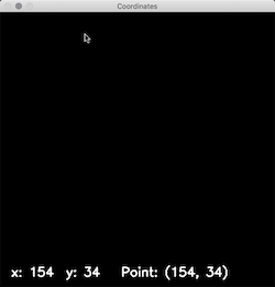\n" ] }, { "cell_type": "code", "execution_count": null, "metadata": {}, "outputs": [], "source": [ "coordinates()" ] }, { "cell_type": "markdown", "metadata": {}, "source": [ "## Draw a Line\n", "\n", "\n",
" The function cv2.line draws a line. It has the following format:\n",
"
\n",
" OpenCV uses BGR color format, which means colors are in the format (<blue>, <green>, <red>), with each going from 0 to 255. We will learn more about color later.\n",
"
\n",
" Exercise: \n",
"
Draw a red (0, 0, 255) line of thickness 5 across the middle of the image.\n",
"
Show the image inline.\n",
"
\n", " It should look like this:\n", "
\n", " \n", "" ] }, { "cell_type": "code", "execution_count": null, "metadata": {}, "outputs": [], "source": [ "img = np.zeros((500, 500, 3), np.uint8) # blank black image\n", "\n", "# TASK #1: Draw a red line of thickness 5 across the middle of the image you saved before\n", "\n", "\n", "# TASK #2: Show the image inline\n", "\n" ] }, { "cell_type": "markdown", "metadata": {}, "source": [ "## Draw a Circle\n", "\n", "\n",
" The function cv2.circle draws a circle. It has the following format:\n",
"
\n",
" For a circle and other closed shapes, a thickness of -1 fills in the shape.\n",
"
\n",
" Exercise:\n",
"
Draw a filled-in blue (255, 0, 0) circle of radius 100 in the top right corner of the image.\n",
"
Show the image inline.\n",
"
\n", " It should look like this:\n", "
\n", " \n", "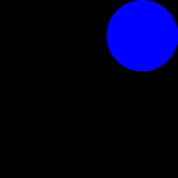\n" ] }, { "cell_type": "code", "execution_count": null, "metadata": { "scrolled": true }, "outputs": [], "source": [ "img = np.zeros((500, 500, 3), np.uint8) # blank black image\n", "\n", "# TASK #1: Draw a blue filled in circle in the top right corner\n", "\n", "\n", "# TASK #2: Show the image inline\n", "\n" ] }, { "cell_type": "markdown", "metadata": {}, "source": [ "## Draw a Rectangle\n", "\n", "\n",
" The function cv2.rectangle draws a rectangle. It has the following format:\n",
"
\n",
" Exercise: \n",
"
Draw a green (0,255,0) rectangle of thickness 50 around the border of the entire image.\n",
"
Show the image inline. \n",
"
\n", " It should look like this:\n", "
\n", "\n", "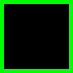" ] }, { "cell_type": "code", "execution_count": null, "metadata": {}, "outputs": [], "source": [ "img = np.zeros((500, 500, 3), np.uint8) # blank black image\n", "\n", "# TASK #1: Draw a green rectangle of thickness 50 around the image\n", "\n", "\n", "# TASK #2: Show the image inline\n", "\n" ] }, { "cell_type": "markdown", "metadata": {}, "source": [ "## Draw Text\n", "\n", "\n",
" The function cv2.putText draws text. It has the following format:\n",
"
\n",
" Use 0 for to use the default font. Scale means the size of the text. \n",
"
\n", "
\n",
" Exercise: \n",
"
Write the text 'Beaver Works' in white (255, 255, 255) near the center of the image.\n",
"
Use 0 for font, 2 for scale, and 3 for thickness.\n",
"
Show the image inline. \n",
"
\n", " It should look like this:\n", "
\n", "\n", "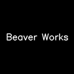" ] }, { "cell_type": "code", "execution_count": null, "metadata": {}, "outputs": [], "source": [ "img = np.zeros((500, 500, 3), np.uint8) # blank black image\n", "\n", "# TASK #1: Draw a green rectangle of thickness 50 around the image\n", "\n", "\n", "# TASK #2: Show the image inline\n", "\n" ] }, { "cell_type": "markdown", "metadata": {}, "source": [ "## Let's Draw Mickey Mouse!!\n", "\n", "\n", " Using the tools we have learned, let's draw Mickey Mouse!\n", "
\n", "\n", "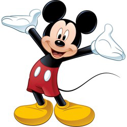\n", "\n", "\n",
" Exercise: \n",
"
You can choose to draw only his head, or part of his body. \n",
"
\n", " Follow these steps:\n", "
- \n",
"
- Sketch your design by hand. Use only lines, circles, and rectangles. \n", "
- Write down which functions and parameters you will use. \n", "
- Type in each function one by one.\n", "
- Show your image inline as you work, making adjustments as needed. \n", "
\n", " Color codes:\n", "
- \n",
"
- Black:
(0,0,0)\n",
" - White:
(255,255,255)\n",
" - Blue:
(255,0,0)\n",
" - Green:
(0,255,0)\n",
" - Red:
(0,0,255)\n",
" - Yellow:
(0,255,255)\n",
"
\n", " Note: This time we created a blank white image to start.\n", "
" ] }, { "cell_type": "code", "execution_count": null, "metadata": { "scrolled": true }, "outputs": [], "source": [ "img = np.full((500, 500, 3), (255,255,255), np.uint8) # blank white image\n", "\n", "# TASK #1: Create Mickey Mouse using the functions we have learned!\n", "\n", "\n", "\n", "# TASK #2: Show your image inline\n", "\n" ] } ], "metadata": { "kernelspec": { "display_name": "Python 3", "language": "python", "name": "python3" }, "language_info": { "codemirror_mode": { "name": "ipython", "version": 3 }, "file_extension": ".py", "mimetype": "text/x-python", "name": "python", "nbconvert_exporter": "python", "pygments_lexer": "ipython3", "version": "3.8.1" } }, "nbformat": 4, "nbformat_minor": 4 }