""" end # ╔═╡ 83ad05a0-2cfb-11eb-1467-e1196985519a md""" #### Advection & diffusion Notice that both functions have a main method with the following signature: `(::Array{Float64,2}, ::ClimateModel)` _maps to_ `::Array{Float64,2}`. As we will see later, `ClimateModel` contains the grid, the velocity vector field and the simulation parameters. """ # ╔═╡ 1e8d37ee-2a97-11eb-1d45-6b426b25d4eb xgrad_kernel = OffsetArray(reshape([-1., 0, 1.], 1, 3), 0:0, -1:1); # ╔═╡ 682f2530-2a97-11eb-3ee6-99a7c79b3767 ygrad_kernel = OffsetArray(reshape([-1., 0, 1.], 3, 1), -1:1, 0:0); # ╔═╡ b629d89a-2a95-11eb-2f27-3dfa45789be4 xdiff_kernel = OffsetArray(reshape([1., -2., 1.], 1, 3), 0:0, -1:1); # ╔═╡ a8d8f8d2-2cfa-11eb-3c3e-d54f7b32e4a2 ydiff_kernel = OffsetArray(reshape([1., -2., 1.], 3, 1), -1:1, 0:0); # ╔═╡ 2beb6ec0-2dcc-11eb-1768-0b8e4fba1597 "Surround an array with one layer of zeros." function pad_zeros(A::AbstractArray{T,N}) where {T,N} PaddedView( zero(T), A, size(A) .+ 2, Tuple(fill(2,N)) ) end # ╔═╡ 13eb3966-2a9a-11eb-086c-05510a3f5b80 md""" #### Data structures Let's look at our first type, `Grid`. Notice that it only has one 'constructor function', which takes `N` (number of longitudinal grid points) and `L` (longitudinal size in meters) as arguments. The struct contains more fields, these are precomputed and stored for performance. """ # ╔═╡ cd2ee4ca-2a06-11eb-0e61-e9a2ecf72bd6 begin struct Grid N::Int64 L::Float64 Δx::Float64 Δy::Float64 x::Array{Float64, 2} y::Array{Float64, 2} Nx::Int64 Ny::Int64 # constructor function: function Grid(N, L) Δx = L/N # [m] Δy = L/N # [m] x = 0. -Δx/2.:Δx:L +Δx/2. x = reshape(x, (1, size(x,1))) y = -L -Δy/2.:Δy:L +Δy/2. y = reshape(y, (size(y,1), 1)) Nx, Ny = size(x, 2), size(y, 1) return new(N, L, Δx, Δy, x, y, Nx, Ny) end end Base.zeros(G::Grid) = zeros(G.Ny, G.Nx) end # ╔═╡ e7f563f0-2d04-11eb-036d-992da68470a6 Grid(5,300.0e3) # ╔═╡ 39404240-2cfe-11eb-2e3c-710e37f8cd4b md""" Next, let's look at three types. Two structs: `OceanModel` and `OceanModelParameters`, and an abstract type: `ClimateModel`. """ # ╔═╡ 0d63e6b2-2b49-11eb-3413-43977d299d90 Base.@kwdef struct OceanModelParameters κ::Float64=1.e4 end # ╔═╡ c9171c56-2dd8-11eb-189b-95d964a9724a abstract type ClimateModel end # ╔═╡ f4c884fc-2a97-11eb-1ba9-01bf579f8b43 begin # main method: advect(T::Array{Float64,2}, O::ClimateModel) = advect(T, O.u, O.v, O.grid.Δy, O.grid.Δx) # helper methods: advect(T::Array{Float64,2}, u, v, Δy, Δx) = pad_zeros([ advect(T, u, v, Δy, Δx, j, i) for j=2:size(T, 1)-1, i=2:size(T, 2)-1 ]) advect(T::Array{Float64,2}, u, v, Δy, Δx, j, i) = .-( u[j, i].*sum(xgrad_kernel[0, -1:1].*T[j, i-1:i+1])/(2Δx) .+ v[j, i].*sum(ygrad_kernel[-1:1, 0].*T[j-1:j+1, i])/(2Δy) ) end # ╔═╡ ee6716c8-2a95-11eb-3a00-319ee69dd37f begin # main method: diffuse(T::Array{Float64,2}, O::ClimateModel) = diffuse(T, O.params.κ, O.grid.Δy, O.grid.Δx) # helper methods: diffuse(T, κ, Δy, Δx) = pad_zeros([ diffuse(T, κ, Δy, Δx, j, i) for j=2:size(T, 1)-1, i=2:size(T, 2)-1 ]) diffuse(T, κ, Δy, Δx, j, i) = κ.*( sum(xdiff_kernel[0, -1:1].*T[j, i-1:i+1])/(Δx^2) + sum(ydiff_kernel[-1:1, 0].*T[j-1:j+1, i])/(Δy^2) ) end # ╔═╡ d3796644-2a05-11eb-11b8-87b6e8c311f9 begin struct OceanModel <: ClimateModel grid::Grid params::OceanModelParameters u::Array{Float64, 2} v::Array{Float64, 2} end OceanModel(G::Grid, params::OceanModelParameters) = OceanModel(G, params, zeros(G), zeros(G)) OceanModel(G::Grid) = OceanModel(G, OceanModelParameters(), zeros(G), zeros(G)) end; # ╔═╡ 5f5e4120-2cfe-11eb-1fa7-99fdd734f7a7 OceanModel <: ClimateModel # it's a subtype! # ╔═╡ 74aa7512-2a9c-11eb-118c-c7a5b60eac1b md""" #### Timestepping The `OceanModel` struct contains a complete _description_ of the model being simulated. The next struct, `ClimateModelSimulation`, contains a _model_, together with the simulation results. It is mutable: timestepping the model means modifying a `ClimateModelSimulation` object. """ # ╔═╡ f92086c4-2a74-11eb-3c72-a1096667183b begin mutable struct ClimateModelSimulation{ModelType<:ClimateModel} model::ModelType T::Array{Float64, 2} Δt::Float64 iteration::Int64 end ClimateModelSimulation(C::ModelType, T, Δt) where ModelType = ClimateModelSimulation{ModelType}(C, T, Δt, 0) end # ╔═╡ 7caca2fa-2a9a-11eb-373f-156a459a1637 function update_ghostcells!(A::Array{Float64,2}; option="no-flux") # Atmp = @view A[:,:] if option=="no-flux" A[1, :] .= A[2, :]; A[end, :] .= A[end-1, :] A[:, 1] .= A[:, 2]; A[:, end] .= A[:, end-1] end end # ╔═╡ 81bb6a4a-2a9c-11eb-38bb-f7701c79afa2 function timestep!(sim::ClimateModelSimulation{OceanModel}) update_ghostcells!(sim.T) tendencies = advect(sim.T, sim.model) .+ diffuse(sim.T, sim.model) sim.T .+= sim.Δt*tendencies sim.iteration += 1 end; # ╔═╡ 31cb0c2c-2a9a-11eb-10ba-d90a00d8e03a md""" #### Exercise 1.1 - _Running the model_ In the next few cells, we set up a simulation. We have included an interactive visualisation of the simulation. 👉 Familiarize yourself with the simulation through interaction. Get a sense for each parameter by changing their values. """ # ╔═╡ 9841ff20-2c06-11eb-3c4c-c34e465e1594 default_grid = Grid(10, 6000.0e3); # ╔═╡ 31cb7aae-2d04-11eb-30cb-a365a6a4aa6b md""" Uncomment (`Ctrl+/` or `Cmd+/`) one of the lines below to choose between the different velocity fields: """ # ╔═╡ 50e89130-2d04-11eb-1c8e-a34775aec40c md""" Choose the initial temperature state: """ # ╔═╡ c7736640-2d04-11eb-1108-59a7446e244d md""" We define our ocean simulation. Run this cell again to reset the simulation to the initial state. """ # ╔═╡ 981ef38a-2a8b-11eb-08be-b94be2924366 md"**Simulation controls**" # ╔═╡ d042d25a-2a62-11eb-33fe-65494bb2fad5 begin quiverBox = @bind show_quiver CheckBox(default=false) anomalyBox = @bind show_anomaly CheckBox(default=false) md""" *Click to show the velocity field* $(quiverBox) *or to show temperature **anomalies** instead of absolute values* $(anomalyBox) """ end # ╔═╡ c20b0e00-2a8a-11eb-045d-9db88411746f begin U_ex_Slider = @bind U_ex Slider(-4:1:8, default=0, show_value=false); md""" $(U_ex_Slider) """ end # ╔═╡ 6dbc3d34-2a89-11eb-2c80-75459a8e237a begin md"*Vary the current speed U:* $(2. ^U_ex) [× reference]" end # ╔═╡ 933d42fa-2a67-11eb-07de-61cab7567d7d begin κ_ex_Slider = @bind κ_ex Slider(0.:1.e3:1.e5, default=1.e4, show_value=true) md""" *Vary the diffusivity κ:* $(κ_ex_Slider) [m²/s] """ end # ╔═╡ c9ea0f72-2a67-11eb-20ba-376ca9c8014f @bind go_ex Clock(0.1) # ╔═╡ c0298712-2a88-11eb-09af-bf2c39167aa6 md"""##### Velocity field for a single circular vortex """ # ╔═╡ e3ee80c0-12dd-11eb-110a-c336bb978c51 begin ∂x(ϕ, Δx) = (ϕ[:,2:end] - ϕ[:,1:end-1])/Δx ∂y(ϕ, Δy) = (ϕ[2:end,:] - ϕ[1:end-1,:])/Δy xpad(ϕ) = hcat(zeros(size(ϕ,1)), ϕ, zeros(size(ϕ,1))) ypad(ϕ) = vcat(zeros(size(ϕ,2))', ϕ, zeros(size(ϕ,2))') xitp(ϕ) = 0.5*(ϕ[:,2:end]+ϕ[:,1:end-1]) yitp(ϕ) = 0.5*(ϕ[2:end,:]+ϕ[1:end-1,:]) function diagnose_velocities(ψ, G) u = xitp(∂y(ψ, G.Δy/G.L)) v = yitp(-∂x(ψ, G.Δx/G.L)) return u,v end end # ╔═╡ df706ebc-2a63-11eb-0b09-fd9f151cb5a8 function impose_no_flux!(u, v) u[1,:] .= 0.; v[1,:] .= 0.; u[end,:] .= 0.; v[end,:] .= 0.; u[:,1] .= 0.; v[:,1] .= 0.; u[:,end] .= 0.; v[:,end] .= 0.; end # ╔═╡ e2e4cfac-2a63-11eb-1b7f-9d8d5d304b43 function PointVortex(G; Ω=1., a=0.2, x0=0.5, y0=0.) x = reshape(0. -G.Δx/(G.L):G.Δx/G.L:1. +G.Δx/(G.L), (1, G.Nx+1)) y = reshape(-1. -G.Δy/(G.L):G.Δy/G.L:1. +G.Δy/(G.L), (G.Ny+1, 1)) function ψ̂(x,y) r = sqrt.((y .-y0).^2 .+ (x .-x0).^2) stream = -Ω/4*r.^2 stream[r .> a] = -Ω*a^2/4*(1. .+ 2*log.(r[r .> a]/a)) return stream end u, v = diagnose_velocities(ψ̂(x, y), G) impose_no_flux!(u, v) return u,v end # ╔═╡ 1dd3fc70-2c06-11eb-27fe-f325ca208504 # ocean_velocities = zeros(default_grid), zeros(default_grid); ocean_velocities = PointVortex(default_grid, Ω=0.5); # ocean_velocities = DoubleGyre(default_grid); # ╔═╡ bb084ace-12e2-11eb-2dfc-111e90eabfdd md"""##### Quasi-realistic ocean velocity field $\vec{u} = (u, v)$ Our velocity field is given by an analytical solution to the classic wind-driven gyre problem, which is given by solving the fourth-order partial differential equation: $- \epsilon_{M} \hat{\nabla}^{4} \hat{\Psi} + \frac{\partial \hat{\Psi} }{ \partial \hat{x}} = \nabla \times \hat{\tau} \mathbf{z},$ where the hats denote that all of the variables have been non-dimensionalized and all of their constant coefficients have been bundles into the single parameter $\epsilon_{M} \equiv \dfrac{\nu}{\beta L^3}$. The solution makes use of an advanced *asymptotic method* (valid in the limit that $\epsilon \ll 1$) known as *boundary layer analysis* (see MIT course 18.305 to learn more). """ # ╔═╡ ecaab27e-2a16-11eb-0e99-87c91e659cf3 function DoubleGyre(G; β=2e-11, τ₀=0.1, ρ₀=1.e3, ν=1.e5, κ=1.e5, H=1000.) ϵM = ν/(β*G.L^3) ϵ = ϵM^(1/3.) x = reshape(0. -G.Δx/(G.L):G.Δx/G.L:1. +G.Δx/(G.L), (1, G.Nx+1)) y = reshape(-1. -G.Δy/(G.L):G.Δy/G.L:1. +G.Δy/(G.L), (G.Ny+1, 1)) ψ̂(x,y) = π*sin.(π*y) * ( 1 .- x - exp.(-x/(2*ϵ)) .* ( cos.(√3*x/(2*ϵ)) .+ (1. /√3)*sin.(√3*x/(2*ϵ)) ) .+ ϵ*exp.((x .- 1.)/ϵ) ) u, v = (τ₀/ρ₀)/(β*G.L*H) .* diagnose_velocities(ψ̂(x, y), G) impose_no_flux!(u, v) return u, v end # ╔═╡ e59d869c-2a88-11eb-2511-5d5b4b380b80 md""" ##### Some simple initial temperature fields """ # ╔═╡ 0ae0bb70-2b8f-11eb-0104-93aa0e1c7a72 constantT(G; value) = zeros(G) .+ value # ╔═╡ c4424838-12e2-11eb-25eb-058344b39c8b linearT(G; value=50.0) = value*0.5*(1. .+[ -(y/G.L) for y in G.y[:, 1], x in G.x[1, :] ]) # ╔═╡ 3d12c114-2a0a-11eb-131e-d1a39b4f440b function InitBox(G; value=50., nx=2, ny=2, xspan=false, yspan=false) T = zeros(G) T[G.Ny÷2-ny:G.Ny÷2+ny, G.Nx÷2-nx:G.Nx÷2+nx] .= value if xspan T[G.Ny÷2-ny:G.Ny÷2+ny, :] .= value end if yspan T[:, G.Nx÷2-nx:G.Nx÷2+nx] .= value end return T end # ╔═╡ 6f19cd80-2c06-11eb-278d-178c1590856f # ocean_T_init = InitBox(default_grid; value=50); ocean_T_init = InitBox(default_grid, value=50, xspan=true); # ocean_T_init = linearT(default_grid); # ╔═╡ 863a6330-2a08-11eb-3992-c3db439fb624 ocean_sim = let P = OceanModelParameters(κ=κ_ex) u, v = ocean_velocities model = OceanModel(default_grid, P, u*2. ^U_ex, v*2. ^U_ex) Δt = 12*60*60 ClimateModelSimulation(model, copy(ocean_T_init), Δt) end; # ╔═╡ 6b3b6030-2066-11eb-3343-e19284638efb plot_kernel(A) = heatmap( collect(A), color=:bluesreds, clims=(-maximum(abs.(A)), maximum(abs.(A))), colorbar=false, xticks=false, yticks=false, size=(30+30*size(A, 2), 30+30*size(A, 1)), xaxis=false, yaxis=false ) |> as_svg # ╔═╡ 3dffa000-2db7-11eb-263b-57fa833d5785 md""" 👉 Some parameters have a physical meaning (`κ`, `u` and `v`), while other parameters control our numerical process. Choose two of these _numerical_ parameters, and describe their effect on the simulation's runtime and the simulation's accuracy. """ # ╔═╡ b952d290-2db7-11eb-3fa9-2bc8d77b9fd6 numerical_parameters_observation = md""" Hello! """ # ╔═╡ 88c56350-2c08-11eb-14e9-77e71d749e6d md""" ## **Exercise 2** - _Complexity_ In this class we have restricted ourself to small problems ($N_{t} < 100$ timesteps and $N_{x;\, y} < 30$ spatial grid-cells) so that they can be run interactively on an average computer. In state-of-the-art climate modelling however, the goal is to push the *numerical resolution* $N$ to be as large as possible (the *grid spacing* $\Delta t$ or $\Delta x$ as small as possible), to resolve physical processes that improve the realism of the simulation (see below). """ # ╔═╡ 014495d6-2cda-11eb-05d7-91e5a467647e html"""Click here to download and run the Lecture 23 notebook in a new tab.
 """
# ╔═╡ d6a56496-2cda-11eb-3d54-d7141a49a446
md"""
Here, we provide a simple estimate of the *computational complexity* of climate models, which reveals a substantial challenge to the improvement of climate models.
Our climate model algorithm can be summarized by the recursive formula:
$T_{i,\, j}^{n+1} = T^{n}_{i,j} + \Delta t * \left( \text{tendencies} \right)$
for each time step ``n \in \left\{1, \dots, M \right\}``, and for each grid point ``i \in \left\{1, \dots, N_x \right\}, j \in \left\{1, \dots, N_y \right\}``.
Our goal is to simulate an ocean of fixed size (e.g. ``6000`` km), for a fixed amount of time (e.g. ``100`` years). By choosing smaller ``\Delta t``, ``\Delta x`` and ``\Delta y``, we get a more accurate simulation, but for the same _size_, it requires more steps. i.e.
$M = \mathcal{O}(\Delta t^{-1}) \qquad N_x = \mathcal{O}(\Delta x^{-1}) \qquad N_y = \mathcal{O}(\Delta y^{-1}).$
Now, the _total runtime_ of our simulation is proportional to the number of steps we need to take, which is ``M\cdot N_x \cdot N_y``. For a fixed aspect ratio $N_{y} = 2N_{x}$, we get
$\text{runtime} = \mathcal{O}(M)\mathcal{O}(2N_{x}^{2}) = \mathcal{O}(M)\mathcal{O}(N_{x}^{2}).$
#### Exercise 2.1
For constant ``M``, we want to verify that $\text{runtime} = \mathcal{O}(N_{x}^{2})$ holds for our numerical model.
👉 Write a function `model_runtime` that takes `N` as an argument, and sets up a model with grid of resolution `N`, and returns the runtime of a single `timestep!`.
"""
# ╔═╡ 126bffce-2d0b-11eb-2bfd-bb5d1ad1169b
function runtime(N)
return missing
end
# ╔═╡ 923af680-2d0b-11eb-3f6a-db4bf29bb6a9
md"""
👉 Call your `runtime` function on a range of values for `N`, and use a plot to demonstrate that the predicted runtime complexity holds.
"""
# ╔═╡ af02d23e-2e93-11eb-3547-85d2aa07081b
# ╔═╡ a6811db2-2cdf-11eb-0aac-b1bf7b7d99eb
md"""
#### Exercise 2.2 - _The CFL condition on $\Delta t$_
In Exercise 1, look for the definition of `Δt`. It is currently set to `12*60*60` (12 hours).
👉 Double `Δt` and run the simulation again. You should see that it runs faster, great! Now, keep doubling `Δt` until you see something 'strange'. Describe what you see.
"""
# ╔═╡ 87de1c70-2d0c-11eb-2c22-f76eeca58f33
Δt_doubling_observations = md"""
Hi!
"""
# ╔═╡ 87e59680-2d0c-11eb-03c7-1d845ca6a1a5
md"""
What you experienced is a _numerical instability_ of the discretization method in our simulation. This is not caused by floating point errors -- it is a theoretical limitation of our method.
To ensure the stability of our finite-difference approximation for advection, heat should not be displaced more than one grid cell in a single timestep. Mathematically, we can ensure this by checking that the distance $L_{CFL} \equiv \max(|\vec{u}|) \Delta t$ is significantly less than the width $\Delta x = \Delta y$ of a single grid cell:
$L_{CFL} \equiv \max(|\vec{u}|) \Delta t \ll \Delta x$
or
$\Delta t \ll \frac{\Delta x}{\max(|\vec{u}|) },$
which is known as **the Courant-Freidrichs-Levy (CFL) condition**.
The exact meaning of ``\ll`` here depends on the simulation at hand, but in our case, it means that there is at least an order of magnitude difference:
$\Delta t < 0.1 \frac{\Delta x}{\max(|\vec{u}|) }.$
Given below is a function `CFL_advection` that takes a `ClimateModel` and computes the CFL value: ``{\Delta x} / {\max(|\vec{u}|) }``.
"""
# ╔═╡ ad7b7ed6-2a9c-11eb-06b7-0f5595167575
function CFL_advection(model::ClimateModel)
model.grid.Δx / maximum(sqrt.(model.u.^2 + model.v.^2))
end
# ╔═╡ 7d3bf550-2e68-11eb-3526-cda9ff3f914e
ocean_sim.Δt, 0.1 * CFL_advection(ocean_sim.model)
# ╔═╡ 3e908bf0-2e94-11eb-28de-a3b1b7435492
md"""
👉 Using the interactive simulation of Exercise 1, verify that the CFL condition is (somewhat) true. Increase the magnitude of ``\vec{u}`` until you start to see numerical artefacts. Now, halve the value fo ``\Delta t``, and again, increase the magnitude of ``\vec{u}``. You should find that _halving ``\Delta t`` allows for twice the velocity magnitude_. The same link exists between ``\Delta t`` and ``\Delta x``.
"""
# ╔═╡ cb3e2990-2e67-11eb-2312-61395c479a15
md"""
The CFL inequality states that if we want to decrease the grid spacing $\Delta x$ (or increase the *resolution* $N_{x}$), we also have to decrease the timestep $\Delta t$ by the same factor. In other words, the timestep can not be thought of as fixed -- it depends on the spatial resolution: $\Delta t \equiv \Delta t_{0} \Delta x$. This means that ``M = \mathcal{O}(N_x)``.
Revisiting our complexity equation, we now have
$\text{runtime} = \mathcal{O}(M) \mathcal{O}(N_x^2) = \mathcal{O}(N_x^3).$
In other words, in a 2-D model, **2x the spatial resolution requires 8x the computational power**.
"""
# ╔═╡ 433a9c1e-2ce0-11eb-319c-e9c785b080ce
md"""
#### Exercise 2.3 - _Moore's Law_
In practice, state-of-the-art climate models are 3-D, not 2-D. It turns out that to preserve the aspect ratio of oceanic motions, the *vertical* grid resolution should also be increased $N_{z} \propto N_{x}$, such that in reality the computational complexity of climate models is:
$\text{runtime} = \mathcal{O}(N_{x}^4).$
This is the fundamental challenge of high-performance climate computing: to increase the resolution of the models by a factor of $2$, the model's run-time increases by a factor of $2^4 = 16$.
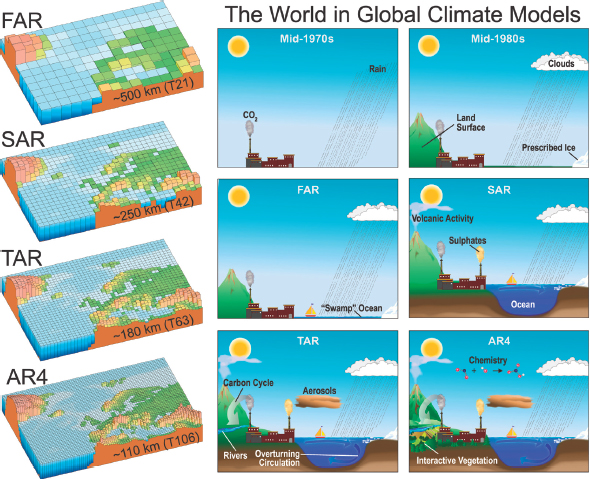
The figure below shows how the grid spacing of state-of-the-art climate models has decreased from $500$ km in 1990 (FAR) to $100$ km in the 2010s (AR4). In other words, grid resolution increased by a factor of $5$ in 20 years.
"""
# ╔═╡ 213f65ce-2ce1-11eb-19d6-5bf5c24d7ed7
html"""
"""
# ╔═╡ d6a56496-2cda-11eb-3d54-d7141a49a446
md"""
Here, we provide a simple estimate of the *computational complexity* of climate models, which reveals a substantial challenge to the improvement of climate models.
Our climate model algorithm can be summarized by the recursive formula:
$T_{i,\, j}^{n+1} = T^{n}_{i,j} + \Delta t * \left( \text{tendencies} \right)$
for each time step ``n \in \left\{1, \dots, M \right\}``, and for each grid point ``i \in \left\{1, \dots, N_x \right\}, j \in \left\{1, \dots, N_y \right\}``.
Our goal is to simulate an ocean of fixed size (e.g. ``6000`` km), for a fixed amount of time (e.g. ``100`` years). By choosing smaller ``\Delta t``, ``\Delta x`` and ``\Delta y``, we get a more accurate simulation, but for the same _size_, it requires more steps. i.e.
$M = \mathcal{O}(\Delta t^{-1}) \qquad N_x = \mathcal{O}(\Delta x^{-1}) \qquad N_y = \mathcal{O}(\Delta y^{-1}).$
Now, the _total runtime_ of our simulation is proportional to the number of steps we need to take, which is ``M\cdot N_x \cdot N_y``. For a fixed aspect ratio $N_{y} = 2N_{x}$, we get
$\text{runtime} = \mathcal{O}(M)\mathcal{O}(2N_{x}^{2}) = \mathcal{O}(M)\mathcal{O}(N_{x}^{2}).$
#### Exercise 2.1
For constant ``M``, we want to verify that $\text{runtime} = \mathcal{O}(N_{x}^{2})$ holds for our numerical model.
👉 Write a function `model_runtime` that takes `N` as an argument, and sets up a model with grid of resolution `N`, and returns the runtime of a single `timestep!`.
"""
# ╔═╡ 126bffce-2d0b-11eb-2bfd-bb5d1ad1169b
function runtime(N)
return missing
end
# ╔═╡ 923af680-2d0b-11eb-3f6a-db4bf29bb6a9
md"""
👉 Call your `runtime` function on a range of values for `N`, and use a plot to demonstrate that the predicted runtime complexity holds.
"""
# ╔═╡ af02d23e-2e93-11eb-3547-85d2aa07081b
# ╔═╡ a6811db2-2cdf-11eb-0aac-b1bf7b7d99eb
md"""
#### Exercise 2.2 - _The CFL condition on $\Delta t$_
In Exercise 1, look for the definition of `Δt`. It is currently set to `12*60*60` (12 hours).
👉 Double `Δt` and run the simulation again. You should see that it runs faster, great! Now, keep doubling `Δt` until you see something 'strange'. Describe what you see.
"""
# ╔═╡ 87de1c70-2d0c-11eb-2c22-f76eeca58f33
Δt_doubling_observations = md"""
Hi!
"""
# ╔═╡ 87e59680-2d0c-11eb-03c7-1d845ca6a1a5
md"""
What you experienced is a _numerical instability_ of the discretization method in our simulation. This is not caused by floating point errors -- it is a theoretical limitation of our method.
To ensure the stability of our finite-difference approximation for advection, heat should not be displaced more than one grid cell in a single timestep. Mathematically, we can ensure this by checking that the distance $L_{CFL} \equiv \max(|\vec{u}|) \Delta t$ is significantly less than the width $\Delta x = \Delta y$ of a single grid cell:
$L_{CFL} \equiv \max(|\vec{u}|) \Delta t \ll \Delta x$
or
$\Delta t \ll \frac{\Delta x}{\max(|\vec{u}|) },$
which is known as **the Courant-Freidrichs-Levy (CFL) condition**.
The exact meaning of ``\ll`` here depends on the simulation at hand, but in our case, it means that there is at least an order of magnitude difference:
$\Delta t < 0.1 \frac{\Delta x}{\max(|\vec{u}|) }.$
Given below is a function `CFL_advection` that takes a `ClimateModel` and computes the CFL value: ``{\Delta x} / {\max(|\vec{u}|) }``.
"""
# ╔═╡ ad7b7ed6-2a9c-11eb-06b7-0f5595167575
function CFL_advection(model::ClimateModel)
model.grid.Δx / maximum(sqrt.(model.u.^2 + model.v.^2))
end
# ╔═╡ 7d3bf550-2e68-11eb-3526-cda9ff3f914e
ocean_sim.Δt, 0.1 * CFL_advection(ocean_sim.model)
# ╔═╡ 3e908bf0-2e94-11eb-28de-a3b1b7435492
md"""
👉 Using the interactive simulation of Exercise 1, verify that the CFL condition is (somewhat) true. Increase the magnitude of ``\vec{u}`` until you start to see numerical artefacts. Now, halve the value fo ``\Delta t``, and again, increase the magnitude of ``\vec{u}``. You should find that _halving ``\Delta t`` allows for twice the velocity magnitude_. The same link exists between ``\Delta t`` and ``\Delta x``.
"""
# ╔═╡ cb3e2990-2e67-11eb-2312-61395c479a15
md"""
The CFL inequality states that if we want to decrease the grid spacing $\Delta x$ (or increase the *resolution* $N_{x}$), we also have to decrease the timestep $\Delta t$ by the same factor. In other words, the timestep can not be thought of as fixed -- it depends on the spatial resolution: $\Delta t \equiv \Delta t_{0} \Delta x$. This means that ``M = \mathcal{O}(N_x)``.
Revisiting our complexity equation, we now have
$\text{runtime} = \mathcal{O}(M) \mathcal{O}(N_x^2) = \mathcal{O}(N_x^3).$
In other words, in a 2-D model, **2x the spatial resolution requires 8x the computational power**.
"""
# ╔═╡ 433a9c1e-2ce0-11eb-319c-e9c785b080ce
md"""
#### Exercise 2.3 - _Moore's Law_
In practice, state-of-the-art climate models are 3-D, not 2-D. It turns out that to preserve the aspect ratio of oceanic motions, the *vertical* grid resolution should also be increased $N_{z} \propto N_{x}$, such that in reality the computational complexity of climate models is:
$\text{runtime} = \mathcal{O}(N_{x}^4).$
This is the fundamental challenge of high-performance climate computing: to increase the resolution of the models by a factor of $2$, the model's run-time increases by a factor of $2^4 = 16$.
The figure below shows how the grid spacing of state-of-the-art climate models has decreased from $500$ km in 1990 (FAR) to $100$ km in the 2010s (AR4). In other words, grid resolution increased by a factor of $5$ in 20 years.
"""
# ╔═╡ 213f65ce-2ce1-11eb-19d6-5bf5c24d7ed7
html"""
 """
# ╔═╡ fced660c-2cd9-11eb-1737-0110789f429e
md"""
Moore's law is the observation that the number of transistors in a dense integrated circuit doubles about every two years. In the context of climate modelling, we can interpret this as meaning that the computational complexity allowed by our best high-performance computers $\mathcal{C}$ doubles every two years:
$\mathcal{C}(t) = \mathcal{C}(2020) * 2^{(t-2020)/2}$
Present-day simulations have a grid spacing of $\Delta x = 30$ km (or about $N_{x} = L/\Delta x \approx \frac{20000\text{ km}}{30\text{ km}} \approx 700$).
👉 By extrapolating Moore's law forward into the future, estimate how long it would take for $\Delta x$ to reach to the $500$ meter scale of clouds, one of the important climate processes ($N_{x} = L/\Delta x \approx 40 000$).
"""
# ╔═╡ 299d5540-2e6a-11eb-2698-05e889127454
cloud_resolution_possible_at = let
missing
end
# ╔═╡ 545cf530-2b48-11eb-378c-3f8eeb89bcba
md"""
## **Exercise 3** - _Radiation_
In Homework 9, we used a **zero-dimensional (0-D)** Energy Balance Model (EBM) to understand how Earth's average radiative imbalance results in temperature changes:
$\begin{split}
C\frac{\partial T}{\partial t} =&\ \hphantom{+}
\frac{S(1 - \alpha)}{4}
&\qquad\text{(absorbed radiation)}
\\
&- (A - BT)
&\qquad\text{(outgoing radiation)}
\end{split}$
This week we will do the same, but now in **two-dimensions (2-D)**, where in addition to heat being added or removed from the system by radiation, heat can be *transported around the system* by oceanic **advection** and **diffusion** (see also Lectures 22 & 23 for 1-D and 2-D advection-diffusion). The governing equation for temperature $T(x,y,t)$ in our coupled climate model is:
$\begin{split}
\frac{\partial T}{\partial t} = & \hphantom{+}
u(x,y) \frac{\partial T}{\partial x} + v(x,y) \frac{\partial T}{\partial y}
&\qquad\text{(advection)}
\\
& + \kappa \left( \frac{\partial^{2} T}{\partial x^{2}} + \frac{\partial^{2} T}{\partial y^{2}} \right)
&\qquad\text{(diffusion)}
\\
& + \frac{S(x,y)(1 - \alpha(T))}{4C}
&\qquad\text{(absorbed radiation)}
\\
& - \frac{(A - BT)}{C}.
&\qquad\text{(outgoing radiation)}
\end{split}$
"""
# ╔═╡ 705ddb90-2d8d-11eb-0c78-13eea6a2df38
md"""
##### Parameters
Below we define two new types: `RadiationOceanModel` and `RadiationOceanModelParameters`. Notice the similarities and differences with our original model. By making `RadiationOceanModel` also a subtype of `ClimateModel`, we will be able to re-use much of our original code.
"""
# ╔═╡ 57535c60-2b49-11eb-07cc-ffc5b4d1f13c
Base.@kwdef struct RadiationOceanModelParameters
κ::Float64=4.e4
C::Float64=51.0 * 60*60*24*365.25 # converted from [W*year/m^2/K] to [J/m^2/K]
A::Float64=210
B::Float64=-1.3
S_mean::Float64 = 1380
α0::Float64=0.3
αi::Float64=0.55
ΔT::Float64=2.0
end
# ╔═╡ 90e1aa00-2b48-11eb-1a2d-8701a3069e50
begin
struct RadiationOceanModel <: ClimateModel
grid::Grid
params::RadiationOceanModelParameters
u::Array{Float64, 2}
v::Array{Float64, 2}
end
RadiationOceanModel(G::Grid, P::RadiationOceanModelParameters, u, v) =
RadiationOceanModel(G, P, u, v)
RadiationOceanModel(G::Grid, P::RadiationOceanModelParameters) =
RadiationOceanModel(G, P, zeros(G), zeros(G))
RadiationOceanModel(G::Grid) =
RadiationOceanModel(G, RadiationOceanModelParameters(), zeros(G), zeros(G))
end;
# ╔═╡ e5b95760-2d98-11eb-0ea3-8bfcf07031d6
md"""
Notice that this struct has `Base.@kwdef` in front of its definition. This allows us to:
1. assign default values to the struct fields, directly inside the definition, and
2. automatically create an easier constructor function that takes _keyword arguments:_
"""
# ╔═╡ adf007c2-2d98-11eb-3004-dfe1b1303454
RadiationOceanModelParameters()
# ╔═╡ be456570-2d98-11eb-0c4e-cd92e0af728b
RadiationOceanModelParameters(S_mean=2000)
# ╔═╡ e80b0532-2b4b-11eb-26fa-cd09eca808bc
md"""
#### Exercise 3.1 - _Absorbed radiation_
The ocean absorbs solar radiation, increasing the temperature. Just like in our EBM model, we model the ocean as a surface with a _temperature-dependent albedo_: ``\alpha(T)``. A high albedo means that more sunlight is reflected, and less is absorbed. We model the albedo function as:
"""
# ╔═╡ 629454e0-2b48-11eb-2ff0-abed400c49f9
function α(T::Float64; α0, αi, ΔT)
if T < -ΔT
return αi
elseif -ΔT <= T < ΔT
return αi + (α0-αi)*(T+ΔT)/(2ΔT)
elseif ΔT <= T
return α0
end
end
# ╔═╡ 287395d0-2dbb-11eb-3ca7-ddcea24a074f
md"""
An area of ocean below 0°C is covered in ice, which is more reflective, and therefore absorbs less solar radiation. In our EBM model, this _positive feedback_ leads to a bifurcation: under the same external conditions, the climate system has multiple equilibria.
In this week's two-dimensional model, the factor ``\alpha`` is also two-dimensional: instead of a global albedo, every grid cell has its own temperature, which determines its own albedo, $\alpha(T(x,y,t))$. We can now have an ocean with warm and cold regions, which absorb different amounts of radiation. The same positive feedback can have a _local_ effect.
Here is a second method for `α` that takes a 2D array `T` with the current ocean temperatures and a `RadiationOceanModel`, and returns the 2D array of albedos. We use the [dot operator](https://docs.julialang.org/en/v1/manual/mathematical-operations/#man-dot-operators) to apply `α` pointwise to `T`, also called _broadcasting_.
"""
# ╔═╡ d63c5fe0-2b49-11eb-07fd-a7ec98af3a89
function α(T::Array{Float64,2}, model::RadiationOceanModel)
α.(T; α0=model.params.α0, αi=model.params.αi, ΔT=model.params.ΔT)
end
# ╔═╡ d9296db0-2dba-11eb-3bb5-9533a338dad8
let
T = -10.0:30.0
plot(
T, α.(T; α0=0.3, αi=0.5, ΔT=2.0),
ylim=(0,1),
ylabel="α (albedo) [unitless]",
xlabel="Temperature [°C]",
)
end
# ╔═╡ 8d729390-2dbc-11eb-0628-f3ed9c9f5ffd
md"""
##### Solar insolation
Our rectangular grid represents the North Atlantic Ocean, stretching from the equator (latitude = 0°) to the North Pole (latitude = 90°) in the latitudinal direction (`y`), and from the east coast of North America to the west coast of Europe in the longitudinal direction (`x`). In reality, climate models have to explicitly deal with the curvature of the Earth when constructing their model grids. Here, we will just treat the North Atlantic Ocean as a rectangle with roughly the correct dimensions.
Just like the albedo, every grid cell will have a local amount of solar insolation. In our model, we use the **annual average** at the latitude of a grid cell $S(y)/4$. This is given by: ([_source_](http://www.atmos.albany.edu/facstaff/brose/classes/ATM623_Spring2015/Notes/Lectures/Lecture11%20--%20Insolation.html))
"""
# ╔═╡ 71f531ae-2dbf-11eb-1d0c-0758eb89bf1d
md"""
_Note that latitude is the horizontal axis in this graph, not the vertical._
"""
# ╔═╡ 0de643d0-2dbf-11eb-3a4c-538c176923f4
function y_to_lat(y::Real; grid::Grid)
π/2 * 0.5 * (y / grid.L + 1.0)
end
# ╔═╡ 2ace4750-2dbe-11eb-0074-0f3a7a929176
function S_at(y::Float64; grid::Grid, S_mean::Float64)
S_mean .* (1+0.5*cos(2 * y_to_lat(y; grid=grid)))
end
# ╔═╡ 5caa4172-2dbe-11eb-2d5a-f5fa621d21a8
let
grid = Grid(50, 6000e3)
params = RadiationOceanModelParameters()
y = grid.y[:]
λ = rad2deg.(y_to_lat.(y; grid=grid))
S = S_at.(y; grid=grid, S_mean=params.S_mean)
p = plot(
λ, S/4,
ylabel="Annual average solar insolation [W/m²]",
xlabel="Latitude [°]",
label=nothing,
lw=3,
ylim=(0,maximum(S/4)*1.05)
)
plot!(p,
λ, fill(params.S_mean/4., size(y)),
linestyle=:dash,
label="Global mean S/4"
)
end
# ╔═╡ 86a004ce-2dd5-11eb-1dca-5702d793ef39
md"""
👉 Write a method `absorbed_solar_radiation` that takes a 2D array `T` with the current ocean temperatures and a `RadiationOceanModel`, and returns the tendencies corresponding to absorbed radiation. This is the analogue of `advect` and `diffuse`.
"""
# ╔═╡ f24e8570-2e6c-11eb-2c21-d319af7cba81
function absorbed_solar_radiation(T::Array{Float64,2}, model::RadiationOceanModel)
return missing
end
# ╔═╡ de7456c0-2b4b-11eb-13c8-01b196821de4
md"""
#### Exercise 3.2 - _Outgoing radiation_
Just like in our EBM from before, when our ocean heats up by absorbing solar radiation, it also _emits radiation back to space_. This **outgoing thermal radiation** is what allows the ocean to eventually come to an equilibrium. The difference here is that each individual grid cell of our model radiatives according to it's local temperature $T_{i,\,j}$.
"""
# ╔═╡ 6745f610-2b48-11eb-2f6c-79e0009dc9c3
function outgoing_thermal_radiation(T; C, A, B)
(A .- B .* (T)) ./ C
end
# ╔═╡ 2274f6b0-2dc5-11eb-10a1-e980bd461ea0
md"""
👉 Write a method `outgoing_termal_radiation` that takes a 2D array `T` with the current ocean temperatures and a `RadiationOceanModel`, and returns the tendencies corresponding to outgoing radiation. This is the analogue of `advect` and `diffuse`.
"""
# ╔═╡ fc55f710-2e6c-11eb-3cea-cfc00c02fc26
function outgoing_thermal_radiation(T::Array{Float64,2}, model::RadiationOceanModel)
return missing
end
# ╔═╡ 6c20ca1e-2b48-11eb-1c3c-418118408c4c
let
params = RadiationOceanModelParameters()
model = RadiationOceanModel(default_grid, params)
plot(
-10:40, outgoing_thermal_radiation(-10:40, A=params.A, B=params.B, C=params.C),
xlabel="Temperature",
ylabel="Outgoing radiation",
label=nothing,
size=(500,250)
)
end
# ╔═╡ fe492480-2b4b-11eb-050e-9b9b2e2bf50f
md"""
#### Exercise 3.3 - _Running the model_
Let's define a new `timestep!` method for our new model. This is exactly the same as our advection-diffusion model, with the addition of the two radiation tendencies.
"""
# ╔═╡ 068795ee-2b4c-11eb-3e58-353eb8978c1c
function timestep!(sim::ClimateModelSimulation{RadiationOceanModel})
update_ghostcells!(sim.T)
tendencies =
advect(sim.T, sim.model) .+
diffuse(sim.T, sim.model) .+
absorbed_solar_radiation(sim.T, sim.model) .-
outgoing_thermal_radiation(sim.T, sim.model)
sim.T .+= sim.Δt*tendencies
sim.iteration += 1
end
# ╔═╡ ad95c4e0-2b4a-11eb-3584-dda89970ffdf
md"""
We can now simulate our radiation ocean model, reusing much of the code from our advection-diffusion simulation.
"""
# ╔═╡ b059c6e0-2b4a-11eb-216a-39bb43c7b423
radiation_sim = let
grid = Grid(10, 6.e6)
# you can specify non-default parameters like so:
# params = RadiationOceanModelParameters(S_mean=1500, A=210, κ=2e4)
params = RadiationOceanModelParameters()
u, v = DoubleGyre(grid)
T_init_value = 10
T_init = constantT(grid; value=T_init_value)
model = RadiationOceanModel(grid, params, u, v)
Δt = 400*60*60
ClimateModelSimulation(model, copy(T_init), Δt)
end
# ╔═╡ 5fd346d0-2b4d-11eb-066b-9ba9c9d97613
@bind go_radiation Clock(.1)
# ╔═╡ 6fc5b760-2e97-11eb-1d7f-0d666b0a41d5
md"""
👉 Play around with the simulation to find the effect of each parameter. In particular, discover the effect of the solar insolation, `S_mean`, the initial temperatures, `T_init`, the liquid and ice albedos: `α0` and `αi`, and the amount of emitted heat at 0°C, `A`.
"""
# ╔═╡ 5a755e00-2e98-11eb-0f83-997a60409484
md"""
#### Exercise 3.4 - _Stable states_
So far, we are able to set up a model and run it interactively. You see that the model quickly goes from the initial temperatures to a _stable state_: a state with balanced energy (radiation out, radiation in). Changing the initial state slightly will probably result in the same stable state.
But let's see what happens when we initialize with extremely high or low initial temperatures...
👉 For ``S=1380`` (present-day value) and default parameters, does `T_init_value=-50` give a different result than `T_init_value=+50`? What about `T_init_value=+55`? By trying various values for `T_init_value`, **how many stable states do you find?**
"""
# ╔═╡ 5294aad0-2d15-11eb-091d-59d7517c4dc2
S_1380_stable_states = md"""
I found ...
"""
# ╔═╡ abd2475e-2d15-11eb-26dc-05253cf65232
md"""
👉 Answer the same question for ``S=1000`` and ``S=2000``.
"""
# ╔═╡ bdd86250-2d15-11eb-0b62-7903ca714312
S_1000_stable_states = md"""
I found ...
"""
# ╔═╡ bed2c7e0-2d15-11eb-14e3-93f5d1b6f3a1
S_2000_stable_states = md"""
I found ...
"""
# ╔═╡ b5703af0-2e98-11eb-1e8c-3d2b51bd9995
md"""
#### Exercise 3.5
That's right, we have found a _bifurcation_! Under the right conditions, there are multiple stable states. But under different conditions, there is only one stable state.
**Hypothesis:** The multiple stable states at ``S = 1380`` are caused by the feedback effect of the ice albedo. A cold ocean reflects more heat and stays cold, a warm ocean absorbs more heat and stays warm.
👉 Find a way to confirm this hypothesis by changing the model parameters in the interactive model. Describe your findings.
"""
# ╔═╡ d9141ca0-2e99-11eb-3ef6-8591c16bb546
albedo_hypothesis_description = md"""
Bonjour !
"""
# ╔═╡ c40b7360-2d15-11eb-0558-d95d615f9b9b
md"""
👉 Why is the number of stable states different for a lower or higher value of ``S``?
"""
# ╔═╡ 02767460-2d16-11eb-2074-07657f84e22d
num_stable_states_answer = md"""
Hi! 🍪
"""
# ╔═╡ 127bcb0e-2c0a-11eb-23df-a75767910fcb
md"""
## **Exercise 4** - _Bifurcation diagram_
So far, we are able to set up a model and run it interactively, and we discovered that by changing the initial value of `S_mean`, we find a different number of stable states.
In this final exercise, we will generate a visualization to help us understand the relationship between `S_mean` and the number of stable states. Instead of running a single model interactively, we write a function that takes the model parameters as input, runs the model until equilibrium, and returns the final mean temperature. We will run this high-level function for various initial values, generating a single graph: the _bifurcation diagram_.
#### Exercise 4.1 - _Equilibrium temperature_
👉 Write a function `eq_T` that takes two argments, `S` and `T_init_value`, that sets up a radiation ocean model with `S` as `S_mean`, and with `T_init_value` as the constant initial temperature. Run the model until you have reached equilibrium (approximately), and return the average temperature.
"""
# ╔═╡ 0d197fe0-2e6d-11eb-2346-2daf4e80a9a7
function eq_T(S, T_init_value)
return missing
end
# ╔═╡ f70f52f0-2e9a-11eb-1bab-13c3b7ad3ca4
md"""
👉 Use the function `eq_T` to verify your answer to Exercise 3.4.
"""
# ╔═╡ 59ecd040-2e9c-11eb-05e3-0bc96e9cddec
# ╔═╡ 2495e330-2c0a-11eb-3a10-530f8b87a4eb
md"""
#### Exercise 4.2
👉 Make a bifurcation diagram. For a couple of pairs `(S,T_init)`, calculate the equilibrium temperature. Create a scatter plot with ``S`` on the horizontal axis, and ``T_{\text{equilibrium}}`` on the vertical.
> This calculation can take quite some time. Some tips:
> 1. Start out with a small amount of points.
> 1. Run the `eq_T` calculations in one cell, and store the result as a vector. Generate the scatter plot in a different cell.
> 1. You can replace a `map` with `ThreadsX.map` to run it in parallel across multiple CPU cores. More on this [below](#threadsx).
"""
# ╔═╡ 59da0470-2b8f-11eb-098c-993effcedecf
# you can change me!
bifurcation_ST = [(S,T) for S in [1000, 1380, 2000] for T in [-50, 0, 50]]
# ╔═╡ 9eacf3d0-2e9d-11eb-3c19-1dcfadccf18d
# ╔═╡ 9e653c70-2e9d-11eb-0af5-25dc140d5824
# ╔═╡ 92ae22de-2d88-11eb-1d03-2977c539ba23
md"""
$(html"")
##### Parallelize a `map`
You use `map` to apply a function to each element of a vector. Why not use a `for` loop? One nice property of `map` code is that you only describe the operation for each element, not the order to run the operations in. This means that it can be _easily parallelized_ by the computer. For example, on a computer with 4 cores, the computation `map(sqrt, 1:100)` can be parallelized by handling `1:25` on the first core, `26:50` on the second, etc., at the same time.
In Julia, many functional primitives (`map`, `filter`, `sum`, `maximum`, `all`, and more) have an automatically multithreaded version, in the `ThreadsX.jl` package. As a demo, compare the two cells below. (You can see the runtime in the bottom right of a cell.) You might need to run the cells a second time, the first time includes Julia's compiler doing its thing.
"""
# ╔═╡ 547d92d0-2d88-11eb-18b5-0fc468ae0026
map(1:8) do i
sleep(.1) # to simulate an expensive computation
i ^ 2
end
# ╔═╡ 60bbba90-2d88-11eb-1616-87d6e15c0795
ThreadsX.map(1:8) do i
sleep(.1) # to simulate an expensive computation
i ^ 2
end
# ╔═╡ 57b6e7d0-2c07-11eb-16c1-0d058a34c7ee
md"""
## **Exercise XX:** _Lecture transcript_
_(MIT students only)_
Please see the link for the transcript document on [Canvas](https://canvas.mit.edu/courses/5637).
We want each of you to correct about 500 lines, but don’t spend more than 20 minutes on it.
See the the beginning of the document for more instructions.
👉 Please mention the name of the video(s) and the line ranges you edited:
"""
# ╔═╡ 57c0d2e0-2c07-11eb-1091-15fec09c4e8b
lines_i_edited = md"""
Abstraction, lines 1-219; Array Basics, lines 1-137; Course Intro, lines 1-144 (_for example_)
"""
# ╔═╡ 57cdcb30-2c07-11eb-39b2-2f225acf589d
if student.name == "Jazzy Doe" || student.kerberos_id == "jazz"
md"""
!!! danger "Before you submit"
Remember to fill in your **name** and **Kerberos ID** at the top of this notebook.
"""
end
# ╔═╡ a04d3dee-2a9c-11eb-040e-7bd2facb2eaa
md"""
# Appendix
"""
# ╔═╡ 0a6e6ad2-2c01-11eb-3151-3d58bc09bc69
ice_gradient = PlotUtils.ContinuousColorGradient([
RGB(0.95, 0.95, 1.0), # sliver of white
RGB(0.05, 0.0, 0.3),
RGB(0.1, 0.05, 0.4),
RGB(0.4, 0.4, 0.5),
RGB(0.95, 0.7, 0.4),
RGB(1.0, 0.9, 0.3)
], [0.0, 0.001, 0.2, 0.5, 0.8, 1.0])
# ╔═╡ c0e46442-27fb-11eb-2c94-15edbda3f84d
function plot_state(sim::ClimateModelSimulation; clims=(-1.1,1.1),
show_quiver=true, show_anomaly=false, IC=nothing)
model = sim.model
grid = sim.model.grid
p = plot(;
xlabel="longitudinal distance [km]", ylabel="latitudinal distance [km]",
clabel="Temperature",
yticks=( (-grid.L:1000e3:grid.L), Int64.(1e-3*(-grid.L:1000e3:grid.L)) ),
xticks=( (0:1000e3:grid.L), Int64.(1e-3*(0:1000e3:grid.L)) ),
xlims=(0., grid.L), ylims=(-grid.L, grid.L),
)
X = repeat(grid.x, grid.Ny, 1)
Y = repeat(grid.y, 1, grid.Nx)
if show_anomaly
arrow_col = :black
maxdiff = maximum(abs.(sim.T .- IC))
heatmap!(p, grid.x[:], grid.y[:], sim.T .- IC, clims=(-1.1, 1.1),
color=:balance, colorbar_title="Temperature anomaly [°C]", linewidth=0.,
size=(400,530)
)
else
arrow_col = :white
heatmap!(p, grid.x[:], grid.y[:], sim.T,
color=ice_gradient, levels=clims[1]:(clims[2]-clims[1])/21.:clims[2],
colorbar_title="Temperature [°C]", clims=clims,
linewidth=0., size=(400,520)
)
end
annotate!(p,
50e3, 6170e3,
text(
string("t = ", Int64(round(sim.iteration*sim.Δt/(60*60*24))), " days"),
color=:black, :left, 9
)
)
annotate!(p,
3000e3, 6170e3,
text(
"mean(T) = $(round(mean(sim.T), digits=1)) °C",
color=:black, :left, 9
)
)
if show_quiver
Nq = grid.N ÷ 5
quiver!(p,
X[(Nq+1)÷2:Nq:end], Y[(Nq+1)÷2:Nq:end],
quiver=grid.L*4 .*(model.u[(Nq+1)÷2:Nq:end], model.v[(Nq+1)÷2:Nq:end]),
color=arrow_col, alpha=0.7
)
end
as_png(p)
end
# ╔═╡ 3b24e1b0-2b46-11eb-383b-c57cbf3e68f1
let
go_ex
if ocean_sim.iteration == 0
timestep!(ocean_sim)
else
for i in 1:50
timestep!(ocean_sim)
end
end
plot_state(ocean_sim, clims=(-10, 40), show_quiver=show_quiver, show_anomaly=show_anomaly, IC=ocean_T_init)
end
# ╔═╡ 6568b850-2b4d-11eb-02e9-696654ac2d37
let
go_radiation
for i in 1:100
timestep!(radiation_sim)
end
plot_state(radiation_sim; clims=(-0,50))
end
# ╔═╡ 57e264a0-2c07-11eb-0e31-2b8fa01be2d1
md"## Function library
Just some helper functions used in the notebook."
# ╔═╡ 57f57770-2c07-11eb-1720-cf00aa7f597b
hint(text) = Markdown.MD(Markdown.Admonition("hint", "Hint", [text]))
# ╔═╡ 171c6880-2d0b-11eb-0180-454f2876cf51
hint(md"""
To measure the runtime of a Julia command, you can do:
```julia
runtime = @elapsed do_something()
```
To get a more precise benchmark, you can average a fixed number of runs, by putting `@elapsed` in front of a `for` loop, for example.
""")
# ╔═╡ ec39a792-2bf7-11eb-11e5-515b39f1adf6
md"""
**How do you determine that the model has reached equilibrium?**
The simplest way is to use the interactive simulation above to find a fixed time/number of steps, for which any initial value has reached equilibrium.
Using a long time period is more accurate, but it means that the runtime will be long. If this is a problem, you can use a dynamic stopping condition instead. For example, you can stop the simulation early when the total incoming and total outgoing radiation are roughly equal.
""" |> hint
# ╔═╡ 590c50c0-2e9b-11eb-2bb2-cf35f65a447e
md"""
Create an array of values for `T_init_value` (not too many!), and run `eq_T` for each. Find clusters in the results.
This is a good opportunity to check whether your implementation of `eq_T` is correct! Use the interactive simulation to check the results manually.
""" |> hint
# ╔═╡ 58094d90-2c07-11eb-2987-15c068fefd8f
almost(text) = Markdown.MD(Markdown.Admonition("warning", "Almost there!", [text]))
# ╔═╡ 581b9d10-2c07-11eb-1e60-c753aa19f4c3
still_missing(text=md"Replace `missing` with your answer.") = Markdown.MD(Markdown.Admonition("warning", "Here we go!", [text]))
# ╔═╡ 582dc580-2c07-11eb-37e3-c32590a0c325
keep_working(text=md"The answer is not quite right.") = Markdown.MD(Markdown.Admonition("danger", "Keep working on it!", [text]))
# ╔═╡ 58403c10-2c07-11eb-1f4b-f9ecb741d881
yays = [md"Fantastic!", md"Splendid!", md"Great!", md"Yay ❤", md"Great! 🎉", md"Well done!", md"Keep it up!", md"Good job!", md"Awesome!", md"You got the right answer!", md"Let's move on to the next section."]
# ╔═╡ 5853eb20-2c07-11eb-18bf-c14ed22ce153
correct(text=rand(yays)) = Markdown.MD(Markdown.Admonition("correct", "Got it!", [text]))
# ╔═╡ 5867e850-2c07-11eb-17d5-9dac155d381b
not_defined(variable_name) = Markdown.MD(Markdown.Admonition("danger", "Oopsie!", [md"Make sure that you define a variable called **$(Markdown.Code(string(variable_name)))**"]))
# ╔═╡ 587b9760-2c07-11eb-17ff-b9e950aa04ac
todo(text) = HTML("""
"""
# ╔═╡ fced660c-2cd9-11eb-1737-0110789f429e
md"""
Moore's law is the observation that the number of transistors in a dense integrated circuit doubles about every two years. In the context of climate modelling, we can interpret this as meaning that the computational complexity allowed by our best high-performance computers $\mathcal{C}$ doubles every two years:
$\mathcal{C}(t) = \mathcal{C}(2020) * 2^{(t-2020)/2}$
Present-day simulations have a grid spacing of $\Delta x = 30$ km (or about $N_{x} = L/\Delta x \approx \frac{20000\text{ km}}{30\text{ km}} \approx 700$).
👉 By extrapolating Moore's law forward into the future, estimate how long it would take for $\Delta x$ to reach to the $500$ meter scale of clouds, one of the important climate processes ($N_{x} = L/\Delta x \approx 40 000$).
"""
# ╔═╡ 299d5540-2e6a-11eb-2698-05e889127454
cloud_resolution_possible_at = let
missing
end
# ╔═╡ 545cf530-2b48-11eb-378c-3f8eeb89bcba
md"""
## **Exercise 3** - _Radiation_
In Homework 9, we used a **zero-dimensional (0-D)** Energy Balance Model (EBM) to understand how Earth's average radiative imbalance results in temperature changes:
$\begin{split}
C\frac{\partial T}{\partial t} =&\ \hphantom{+}
\frac{S(1 - \alpha)}{4}
&\qquad\text{(absorbed radiation)}
\\
&- (A - BT)
&\qquad\text{(outgoing radiation)}
\end{split}$
This week we will do the same, but now in **two-dimensions (2-D)**, where in addition to heat being added or removed from the system by radiation, heat can be *transported around the system* by oceanic **advection** and **diffusion** (see also Lectures 22 & 23 for 1-D and 2-D advection-diffusion). The governing equation for temperature $T(x,y,t)$ in our coupled climate model is:
$\begin{split}
\frac{\partial T}{\partial t} = & \hphantom{+}
u(x,y) \frac{\partial T}{\partial x} + v(x,y) \frac{\partial T}{\partial y}
&\qquad\text{(advection)}
\\
& + \kappa \left( \frac{\partial^{2} T}{\partial x^{2}} + \frac{\partial^{2} T}{\partial y^{2}} \right)
&\qquad\text{(diffusion)}
\\
& + \frac{S(x,y)(1 - \alpha(T))}{4C}
&\qquad\text{(absorbed radiation)}
\\
& - \frac{(A - BT)}{C}.
&\qquad\text{(outgoing radiation)}
\end{split}$
"""
# ╔═╡ 705ddb90-2d8d-11eb-0c78-13eea6a2df38
md"""
##### Parameters
Below we define two new types: `RadiationOceanModel` and `RadiationOceanModelParameters`. Notice the similarities and differences with our original model. By making `RadiationOceanModel` also a subtype of `ClimateModel`, we will be able to re-use much of our original code.
"""
# ╔═╡ 57535c60-2b49-11eb-07cc-ffc5b4d1f13c
Base.@kwdef struct RadiationOceanModelParameters
κ::Float64=4.e4
C::Float64=51.0 * 60*60*24*365.25 # converted from [W*year/m^2/K] to [J/m^2/K]
A::Float64=210
B::Float64=-1.3
S_mean::Float64 = 1380
α0::Float64=0.3
αi::Float64=0.55
ΔT::Float64=2.0
end
# ╔═╡ 90e1aa00-2b48-11eb-1a2d-8701a3069e50
begin
struct RadiationOceanModel <: ClimateModel
grid::Grid
params::RadiationOceanModelParameters
u::Array{Float64, 2}
v::Array{Float64, 2}
end
RadiationOceanModel(G::Grid, P::RadiationOceanModelParameters, u, v) =
RadiationOceanModel(G, P, u, v)
RadiationOceanModel(G::Grid, P::RadiationOceanModelParameters) =
RadiationOceanModel(G, P, zeros(G), zeros(G))
RadiationOceanModel(G::Grid) =
RadiationOceanModel(G, RadiationOceanModelParameters(), zeros(G), zeros(G))
end;
# ╔═╡ e5b95760-2d98-11eb-0ea3-8bfcf07031d6
md"""
Notice that this struct has `Base.@kwdef` in front of its definition. This allows us to:
1. assign default values to the struct fields, directly inside the definition, and
2. automatically create an easier constructor function that takes _keyword arguments:_
"""
# ╔═╡ adf007c2-2d98-11eb-3004-dfe1b1303454
RadiationOceanModelParameters()
# ╔═╡ be456570-2d98-11eb-0c4e-cd92e0af728b
RadiationOceanModelParameters(S_mean=2000)
# ╔═╡ e80b0532-2b4b-11eb-26fa-cd09eca808bc
md"""
#### Exercise 3.1 - _Absorbed radiation_
The ocean absorbs solar radiation, increasing the temperature. Just like in our EBM model, we model the ocean as a surface with a _temperature-dependent albedo_: ``\alpha(T)``. A high albedo means that more sunlight is reflected, and less is absorbed. We model the albedo function as:
"""
# ╔═╡ 629454e0-2b48-11eb-2ff0-abed400c49f9
function α(T::Float64; α0, αi, ΔT)
if T < -ΔT
return αi
elseif -ΔT <= T < ΔT
return αi + (α0-αi)*(T+ΔT)/(2ΔT)
elseif ΔT <= T
return α0
end
end
# ╔═╡ 287395d0-2dbb-11eb-3ca7-ddcea24a074f
md"""
An area of ocean below 0°C is covered in ice, which is more reflective, and therefore absorbs less solar radiation. In our EBM model, this _positive feedback_ leads to a bifurcation: under the same external conditions, the climate system has multiple equilibria.
In this week's two-dimensional model, the factor ``\alpha`` is also two-dimensional: instead of a global albedo, every grid cell has its own temperature, which determines its own albedo, $\alpha(T(x,y,t))$. We can now have an ocean with warm and cold regions, which absorb different amounts of radiation. The same positive feedback can have a _local_ effect.
Here is a second method for `α` that takes a 2D array `T` with the current ocean temperatures and a `RadiationOceanModel`, and returns the 2D array of albedos. We use the [dot operator](https://docs.julialang.org/en/v1/manual/mathematical-operations/#man-dot-operators) to apply `α` pointwise to `T`, also called _broadcasting_.
"""
# ╔═╡ d63c5fe0-2b49-11eb-07fd-a7ec98af3a89
function α(T::Array{Float64,2}, model::RadiationOceanModel)
α.(T; α0=model.params.α0, αi=model.params.αi, ΔT=model.params.ΔT)
end
# ╔═╡ d9296db0-2dba-11eb-3bb5-9533a338dad8
let
T = -10.0:30.0
plot(
T, α.(T; α0=0.3, αi=0.5, ΔT=2.0),
ylim=(0,1),
ylabel="α (albedo) [unitless]",
xlabel="Temperature [°C]",
)
end
# ╔═╡ 8d729390-2dbc-11eb-0628-f3ed9c9f5ffd
md"""
##### Solar insolation
Our rectangular grid represents the North Atlantic Ocean, stretching from the equator (latitude = 0°) to the North Pole (latitude = 90°) in the latitudinal direction (`y`), and from the east coast of North America to the west coast of Europe in the longitudinal direction (`x`). In reality, climate models have to explicitly deal with the curvature of the Earth when constructing their model grids. Here, we will just treat the North Atlantic Ocean as a rectangle with roughly the correct dimensions.
Just like the albedo, every grid cell will have a local amount of solar insolation. In our model, we use the **annual average** at the latitude of a grid cell $S(y)/4$. This is given by: ([_source_](http://www.atmos.albany.edu/facstaff/brose/classes/ATM623_Spring2015/Notes/Lectures/Lecture11%20--%20Insolation.html))
"""
# ╔═╡ 71f531ae-2dbf-11eb-1d0c-0758eb89bf1d
md"""
_Note that latitude is the horizontal axis in this graph, not the vertical._
"""
# ╔═╡ 0de643d0-2dbf-11eb-3a4c-538c176923f4
function y_to_lat(y::Real; grid::Grid)
π/2 * 0.5 * (y / grid.L + 1.0)
end
# ╔═╡ 2ace4750-2dbe-11eb-0074-0f3a7a929176
function S_at(y::Float64; grid::Grid, S_mean::Float64)
S_mean .* (1+0.5*cos(2 * y_to_lat(y; grid=grid)))
end
# ╔═╡ 5caa4172-2dbe-11eb-2d5a-f5fa621d21a8
let
grid = Grid(50, 6000e3)
params = RadiationOceanModelParameters()
y = grid.y[:]
λ = rad2deg.(y_to_lat.(y; grid=grid))
S = S_at.(y; grid=grid, S_mean=params.S_mean)
p = plot(
λ, S/4,
ylabel="Annual average solar insolation [W/m²]",
xlabel="Latitude [°]",
label=nothing,
lw=3,
ylim=(0,maximum(S/4)*1.05)
)
plot!(p,
λ, fill(params.S_mean/4., size(y)),
linestyle=:dash,
label="Global mean S/4"
)
end
# ╔═╡ 86a004ce-2dd5-11eb-1dca-5702d793ef39
md"""
👉 Write a method `absorbed_solar_radiation` that takes a 2D array `T` with the current ocean temperatures and a `RadiationOceanModel`, and returns the tendencies corresponding to absorbed radiation. This is the analogue of `advect` and `diffuse`.
"""
# ╔═╡ f24e8570-2e6c-11eb-2c21-d319af7cba81
function absorbed_solar_radiation(T::Array{Float64,2}, model::RadiationOceanModel)
return missing
end
# ╔═╡ de7456c0-2b4b-11eb-13c8-01b196821de4
md"""
#### Exercise 3.2 - _Outgoing radiation_
Just like in our EBM from before, when our ocean heats up by absorbing solar radiation, it also _emits radiation back to space_. This **outgoing thermal radiation** is what allows the ocean to eventually come to an equilibrium. The difference here is that each individual grid cell of our model radiatives according to it's local temperature $T_{i,\,j}$.
"""
# ╔═╡ 6745f610-2b48-11eb-2f6c-79e0009dc9c3
function outgoing_thermal_radiation(T; C, A, B)
(A .- B .* (T)) ./ C
end
# ╔═╡ 2274f6b0-2dc5-11eb-10a1-e980bd461ea0
md"""
👉 Write a method `outgoing_termal_radiation` that takes a 2D array `T` with the current ocean temperatures and a `RadiationOceanModel`, and returns the tendencies corresponding to outgoing radiation. This is the analogue of `advect` and `diffuse`.
"""
# ╔═╡ fc55f710-2e6c-11eb-3cea-cfc00c02fc26
function outgoing_thermal_radiation(T::Array{Float64,2}, model::RadiationOceanModel)
return missing
end
# ╔═╡ 6c20ca1e-2b48-11eb-1c3c-418118408c4c
let
params = RadiationOceanModelParameters()
model = RadiationOceanModel(default_grid, params)
plot(
-10:40, outgoing_thermal_radiation(-10:40, A=params.A, B=params.B, C=params.C),
xlabel="Temperature",
ylabel="Outgoing radiation",
label=nothing,
size=(500,250)
)
end
# ╔═╡ fe492480-2b4b-11eb-050e-9b9b2e2bf50f
md"""
#### Exercise 3.3 - _Running the model_
Let's define a new `timestep!` method for our new model. This is exactly the same as our advection-diffusion model, with the addition of the two radiation tendencies.
"""
# ╔═╡ 068795ee-2b4c-11eb-3e58-353eb8978c1c
function timestep!(sim::ClimateModelSimulation{RadiationOceanModel})
update_ghostcells!(sim.T)
tendencies =
advect(sim.T, sim.model) .+
diffuse(sim.T, sim.model) .+
absorbed_solar_radiation(sim.T, sim.model) .-
outgoing_thermal_radiation(sim.T, sim.model)
sim.T .+= sim.Δt*tendencies
sim.iteration += 1
end
# ╔═╡ ad95c4e0-2b4a-11eb-3584-dda89970ffdf
md"""
We can now simulate our radiation ocean model, reusing much of the code from our advection-diffusion simulation.
"""
# ╔═╡ b059c6e0-2b4a-11eb-216a-39bb43c7b423
radiation_sim = let
grid = Grid(10, 6.e6)
# you can specify non-default parameters like so:
# params = RadiationOceanModelParameters(S_mean=1500, A=210, κ=2e4)
params = RadiationOceanModelParameters()
u, v = DoubleGyre(grid)
T_init_value = 10
T_init = constantT(grid; value=T_init_value)
model = RadiationOceanModel(grid, params, u, v)
Δt = 400*60*60
ClimateModelSimulation(model, copy(T_init), Δt)
end
# ╔═╡ 5fd346d0-2b4d-11eb-066b-9ba9c9d97613
@bind go_radiation Clock(.1)
# ╔═╡ 6fc5b760-2e97-11eb-1d7f-0d666b0a41d5
md"""
👉 Play around with the simulation to find the effect of each parameter. In particular, discover the effect of the solar insolation, `S_mean`, the initial temperatures, `T_init`, the liquid and ice albedos: `α0` and `αi`, and the amount of emitted heat at 0°C, `A`.
"""
# ╔═╡ 5a755e00-2e98-11eb-0f83-997a60409484
md"""
#### Exercise 3.4 - _Stable states_
So far, we are able to set up a model and run it interactively. You see that the model quickly goes from the initial temperatures to a _stable state_: a state with balanced energy (radiation out, radiation in). Changing the initial state slightly will probably result in the same stable state.
But let's see what happens when we initialize with extremely high or low initial temperatures...
👉 For ``S=1380`` (present-day value) and default parameters, does `T_init_value=-50` give a different result than `T_init_value=+50`? What about `T_init_value=+55`? By trying various values for `T_init_value`, **how many stable states do you find?**
"""
# ╔═╡ 5294aad0-2d15-11eb-091d-59d7517c4dc2
S_1380_stable_states = md"""
I found ...
"""
# ╔═╡ abd2475e-2d15-11eb-26dc-05253cf65232
md"""
👉 Answer the same question for ``S=1000`` and ``S=2000``.
"""
# ╔═╡ bdd86250-2d15-11eb-0b62-7903ca714312
S_1000_stable_states = md"""
I found ...
"""
# ╔═╡ bed2c7e0-2d15-11eb-14e3-93f5d1b6f3a1
S_2000_stable_states = md"""
I found ...
"""
# ╔═╡ b5703af0-2e98-11eb-1e8c-3d2b51bd9995
md"""
#### Exercise 3.5
That's right, we have found a _bifurcation_! Under the right conditions, there are multiple stable states. But under different conditions, there is only one stable state.
**Hypothesis:** The multiple stable states at ``S = 1380`` are caused by the feedback effect of the ice albedo. A cold ocean reflects more heat and stays cold, a warm ocean absorbs more heat and stays warm.
👉 Find a way to confirm this hypothesis by changing the model parameters in the interactive model. Describe your findings.
"""
# ╔═╡ d9141ca0-2e99-11eb-3ef6-8591c16bb546
albedo_hypothesis_description = md"""
Bonjour !
"""
# ╔═╡ c40b7360-2d15-11eb-0558-d95d615f9b9b
md"""
👉 Why is the number of stable states different for a lower or higher value of ``S``?
"""
# ╔═╡ 02767460-2d16-11eb-2074-07657f84e22d
num_stable_states_answer = md"""
Hi! 🍪
"""
# ╔═╡ 127bcb0e-2c0a-11eb-23df-a75767910fcb
md"""
## **Exercise 4** - _Bifurcation diagram_
So far, we are able to set up a model and run it interactively, and we discovered that by changing the initial value of `S_mean`, we find a different number of stable states.
In this final exercise, we will generate a visualization to help us understand the relationship between `S_mean` and the number of stable states. Instead of running a single model interactively, we write a function that takes the model parameters as input, runs the model until equilibrium, and returns the final mean temperature. We will run this high-level function for various initial values, generating a single graph: the _bifurcation diagram_.
#### Exercise 4.1 - _Equilibrium temperature_
👉 Write a function `eq_T` that takes two argments, `S` and `T_init_value`, that sets up a radiation ocean model with `S` as `S_mean`, and with `T_init_value` as the constant initial temperature. Run the model until you have reached equilibrium (approximately), and return the average temperature.
"""
# ╔═╡ 0d197fe0-2e6d-11eb-2346-2daf4e80a9a7
function eq_T(S, T_init_value)
return missing
end
# ╔═╡ f70f52f0-2e9a-11eb-1bab-13c3b7ad3ca4
md"""
👉 Use the function `eq_T` to verify your answer to Exercise 3.4.
"""
# ╔═╡ 59ecd040-2e9c-11eb-05e3-0bc96e9cddec
# ╔═╡ 2495e330-2c0a-11eb-3a10-530f8b87a4eb
md"""
#### Exercise 4.2
👉 Make a bifurcation diagram. For a couple of pairs `(S,T_init)`, calculate the equilibrium temperature. Create a scatter plot with ``S`` on the horizontal axis, and ``T_{\text{equilibrium}}`` on the vertical.
> This calculation can take quite some time. Some tips:
> 1. Start out with a small amount of points.
> 1. Run the `eq_T` calculations in one cell, and store the result as a vector. Generate the scatter plot in a different cell.
> 1. You can replace a `map` with `ThreadsX.map` to run it in parallel across multiple CPU cores. More on this [below](#threadsx).
"""
# ╔═╡ 59da0470-2b8f-11eb-098c-993effcedecf
# you can change me!
bifurcation_ST = [(S,T) for S in [1000, 1380, 2000] for T in [-50, 0, 50]]
# ╔═╡ 9eacf3d0-2e9d-11eb-3c19-1dcfadccf18d
# ╔═╡ 9e653c70-2e9d-11eb-0af5-25dc140d5824
# ╔═╡ 92ae22de-2d88-11eb-1d03-2977c539ba23
md"""
$(html"")
##### Parallelize a `map`
You use `map` to apply a function to each element of a vector. Why not use a `for` loop? One nice property of `map` code is that you only describe the operation for each element, not the order to run the operations in. This means that it can be _easily parallelized_ by the computer. For example, on a computer with 4 cores, the computation `map(sqrt, 1:100)` can be parallelized by handling `1:25` on the first core, `26:50` on the second, etc., at the same time.
In Julia, many functional primitives (`map`, `filter`, `sum`, `maximum`, `all`, and more) have an automatically multithreaded version, in the `ThreadsX.jl` package. As a demo, compare the two cells below. (You can see the runtime in the bottom right of a cell.) You might need to run the cells a second time, the first time includes Julia's compiler doing its thing.
"""
# ╔═╡ 547d92d0-2d88-11eb-18b5-0fc468ae0026
map(1:8) do i
sleep(.1) # to simulate an expensive computation
i ^ 2
end
# ╔═╡ 60bbba90-2d88-11eb-1616-87d6e15c0795
ThreadsX.map(1:8) do i
sleep(.1) # to simulate an expensive computation
i ^ 2
end
# ╔═╡ 57b6e7d0-2c07-11eb-16c1-0d058a34c7ee
md"""
## **Exercise XX:** _Lecture transcript_
_(MIT students only)_
Please see the link for the transcript document on [Canvas](https://canvas.mit.edu/courses/5637).
We want each of you to correct about 500 lines, but don’t spend more than 20 minutes on it.
See the the beginning of the document for more instructions.
👉 Please mention the name of the video(s) and the line ranges you edited:
"""
# ╔═╡ 57c0d2e0-2c07-11eb-1091-15fec09c4e8b
lines_i_edited = md"""
Abstraction, lines 1-219; Array Basics, lines 1-137; Course Intro, lines 1-144 (_for example_)
"""
# ╔═╡ 57cdcb30-2c07-11eb-39b2-2f225acf589d
if student.name == "Jazzy Doe" || student.kerberos_id == "jazz"
md"""
!!! danger "Before you submit"
Remember to fill in your **name** and **Kerberos ID** at the top of this notebook.
"""
end
# ╔═╡ a04d3dee-2a9c-11eb-040e-7bd2facb2eaa
md"""
# Appendix
"""
# ╔═╡ 0a6e6ad2-2c01-11eb-3151-3d58bc09bc69
ice_gradient = PlotUtils.ContinuousColorGradient([
RGB(0.95, 0.95, 1.0), # sliver of white
RGB(0.05, 0.0, 0.3),
RGB(0.1, 0.05, 0.4),
RGB(0.4, 0.4, 0.5),
RGB(0.95, 0.7, 0.4),
RGB(1.0, 0.9, 0.3)
], [0.0, 0.001, 0.2, 0.5, 0.8, 1.0])
# ╔═╡ c0e46442-27fb-11eb-2c94-15edbda3f84d
function plot_state(sim::ClimateModelSimulation; clims=(-1.1,1.1),
show_quiver=true, show_anomaly=false, IC=nothing)
model = sim.model
grid = sim.model.grid
p = plot(;
xlabel="longitudinal distance [km]", ylabel="latitudinal distance [km]",
clabel="Temperature",
yticks=( (-grid.L:1000e3:grid.L), Int64.(1e-3*(-grid.L:1000e3:grid.L)) ),
xticks=( (0:1000e3:grid.L), Int64.(1e-3*(0:1000e3:grid.L)) ),
xlims=(0., grid.L), ylims=(-grid.L, grid.L),
)
X = repeat(grid.x, grid.Ny, 1)
Y = repeat(grid.y, 1, grid.Nx)
if show_anomaly
arrow_col = :black
maxdiff = maximum(abs.(sim.T .- IC))
heatmap!(p, grid.x[:], grid.y[:], sim.T .- IC, clims=(-1.1, 1.1),
color=:balance, colorbar_title="Temperature anomaly [°C]", linewidth=0.,
size=(400,530)
)
else
arrow_col = :white
heatmap!(p, grid.x[:], grid.y[:], sim.T,
color=ice_gradient, levels=clims[1]:(clims[2]-clims[1])/21.:clims[2],
colorbar_title="Temperature [°C]", clims=clims,
linewidth=0., size=(400,520)
)
end
annotate!(p,
50e3, 6170e3,
text(
string("t = ", Int64(round(sim.iteration*sim.Δt/(60*60*24))), " days"),
color=:black, :left, 9
)
)
annotate!(p,
3000e3, 6170e3,
text(
"mean(T) = $(round(mean(sim.T), digits=1)) °C",
color=:black, :left, 9
)
)
if show_quiver
Nq = grid.N ÷ 5
quiver!(p,
X[(Nq+1)÷2:Nq:end], Y[(Nq+1)÷2:Nq:end],
quiver=grid.L*4 .*(model.u[(Nq+1)÷2:Nq:end], model.v[(Nq+1)÷2:Nq:end]),
color=arrow_col, alpha=0.7
)
end
as_png(p)
end
# ╔═╡ 3b24e1b0-2b46-11eb-383b-c57cbf3e68f1
let
go_ex
if ocean_sim.iteration == 0
timestep!(ocean_sim)
else
for i in 1:50
timestep!(ocean_sim)
end
end
plot_state(ocean_sim, clims=(-10, 40), show_quiver=show_quiver, show_anomaly=show_anomaly, IC=ocean_T_init)
end
# ╔═╡ 6568b850-2b4d-11eb-02e9-696654ac2d37
let
go_radiation
for i in 1:100
timestep!(radiation_sim)
end
plot_state(radiation_sim; clims=(-0,50))
end
# ╔═╡ 57e264a0-2c07-11eb-0e31-2b8fa01be2d1
md"## Function library
Just some helper functions used in the notebook."
# ╔═╡ 57f57770-2c07-11eb-1720-cf00aa7f597b
hint(text) = Markdown.MD(Markdown.Admonition("hint", "Hint", [text]))
# ╔═╡ 171c6880-2d0b-11eb-0180-454f2876cf51
hint(md"""
To measure the runtime of a Julia command, you can do:
```julia
runtime = @elapsed do_something()
```
To get a more precise benchmark, you can average a fixed number of runs, by putting `@elapsed` in front of a `for` loop, for example.
""")
# ╔═╡ ec39a792-2bf7-11eb-11e5-515b39f1adf6
md"""
**How do you determine that the model has reached equilibrium?**
The simplest way is to use the interactive simulation above to find a fixed time/number of steps, for which any initial value has reached equilibrium.
Using a long time period is more accurate, but it means that the runtime will be long. If this is a problem, you can use a dynamic stopping condition instead. For example, you can stop the simulation early when the total incoming and total outgoing radiation are roughly equal.
""" |> hint
# ╔═╡ 590c50c0-2e9b-11eb-2bb2-cf35f65a447e
md"""
Create an array of values for `T_init_value` (not too many!), and run `eq_T` for each. Find clusters in the results.
This is a good opportunity to check whether your implementation of `eq_T` is correct! Use the interactive simulation to check the results manually.
""" |> hint
# ╔═╡ 58094d90-2c07-11eb-2987-15c068fefd8f
almost(text) = Markdown.MD(Markdown.Admonition("warning", "Almost there!", [text]))
# ╔═╡ 581b9d10-2c07-11eb-1e60-c753aa19f4c3
still_missing(text=md"Replace `missing` with your answer.") = Markdown.MD(Markdown.Admonition("warning", "Here we go!", [text]))
# ╔═╡ 582dc580-2c07-11eb-37e3-c32590a0c325
keep_working(text=md"The answer is not quite right.") = Markdown.MD(Markdown.Admonition("danger", "Keep working on it!", [text]))
# ╔═╡ 58403c10-2c07-11eb-1f4b-f9ecb741d881
yays = [md"Fantastic!", md"Splendid!", md"Great!", md"Yay ❤", md"Great! 🎉", md"Well done!", md"Keep it up!", md"Good job!", md"Awesome!", md"You got the right answer!", md"Let's move on to the next section."]
# ╔═╡ 5853eb20-2c07-11eb-18bf-c14ed22ce153
correct(text=rand(yays)) = Markdown.MD(Markdown.Admonition("correct", "Got it!", [text]))
# ╔═╡ 5867e850-2c07-11eb-17d5-9dac155d381b
not_defined(variable_name) = Markdown.MD(Markdown.Admonition("danger", "Oopsie!", [md"Make sure that you define a variable called **$(Markdown.Code(string(variable_name)))**"]))
# ╔═╡ 587b9760-2c07-11eb-17ff-b9e950aa04ac
todo(text) = HTML("""