---
title: 'STA130 - Class #3: How R You?'
author: "Nathan Taback"
date: '2018-01-22'
output:
ioslides_presentation:
widescreen: true
smaller: true
---
```{r setup, include=FALSE}
knitr::opts_chunk$set(echo = TRUE, warning = FALSE, message = FALSE)
library(tidyverse)
```
## Today's Class
- RStudio user interface
- R Objects
- R Functions
- R Scripts
- R Packages
- R Lists
- R Notation
- R Missing Data
- dplyr
## Announcements
- Tutorial grades will be assigned according to the following marking scheme.
| | Mark |
|------------------------------------|------|
| Attendance for the entire tutorial | 1 |
| Assigned homework completion^a^ | 1 |
| In-class exercises | 4 |
| Total | 6 |
- You will learn about the mentorship program in this week's tutorial (3% of final grade).
## RStudio User Interface
 ## R Objects
- R lets you save data by storing it inside an R object.
- What’s an object? Just a name that you can use to call up stored data.
```{r}
x <- 1
x
```
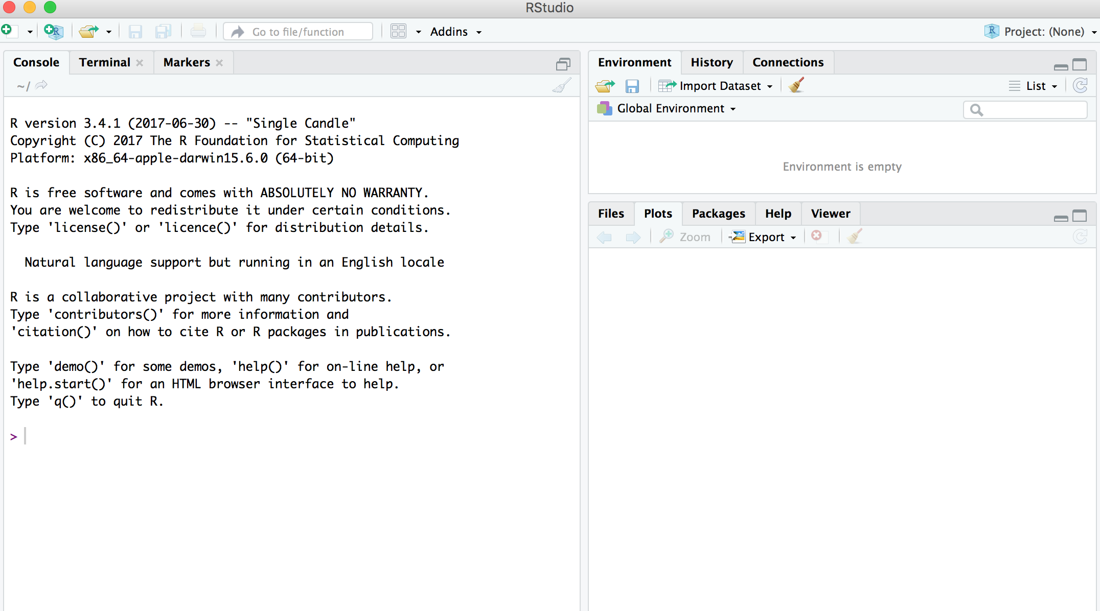
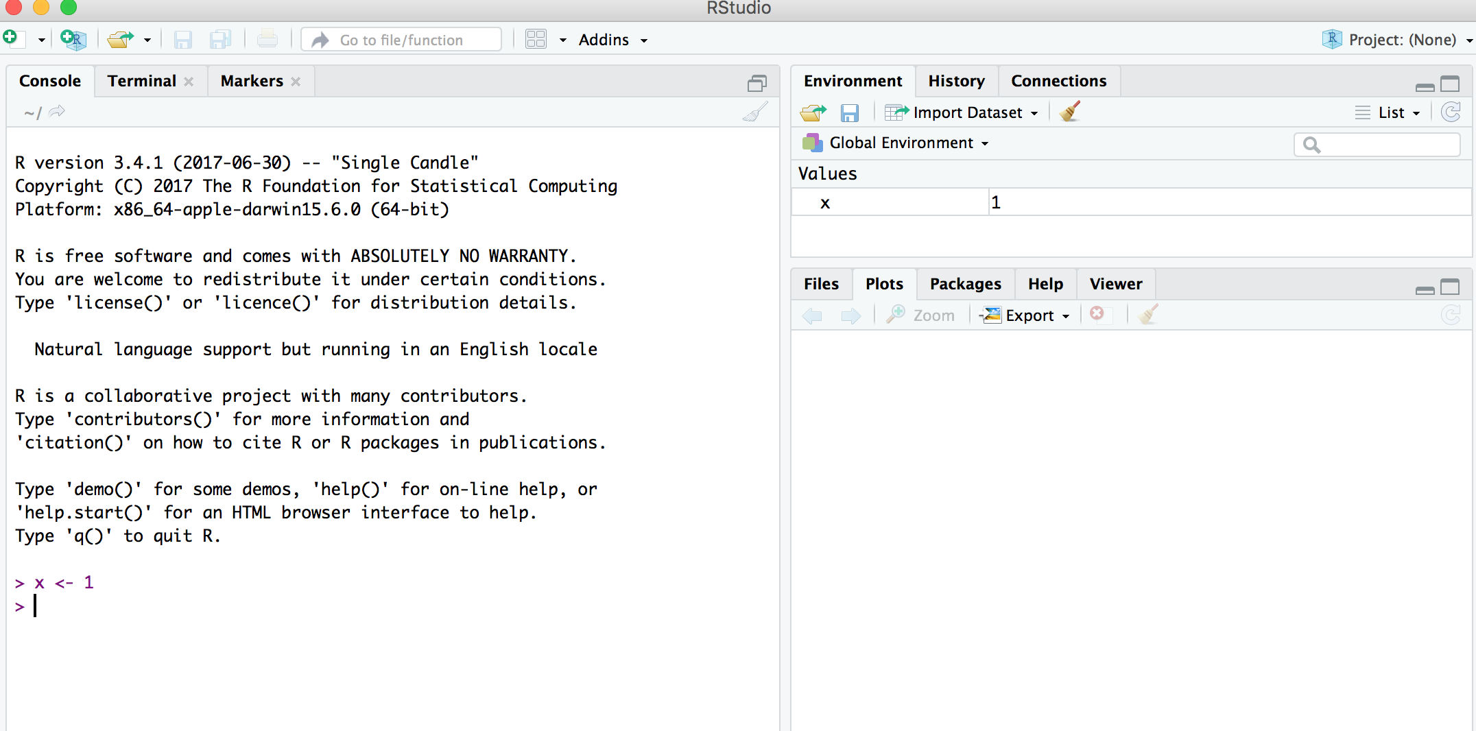
## Environment Pane in RStudio
- When you create an object, the object will appear in the environment pane of RStudio.
## R Objects
- R lets you save data by storing it inside an R object.
- What’s an object? Just a name that you can use to call up stored data.
```{r}
x <- 1
x
```
## Environment Pane in RStudio
- When you create an object, the object will appear in the environment pane of RStudio.
 ## Functions
- R comes with many functions that you can use to do sophisticated tasks like random sampling.
- For example, you can round a number with the round function `round()`, or calculate its absolute value with `abs()`.
- Write the name of the function and then the data you want the function to operate on in parentheses:
```{r}
round(-2.718282, 2)
abs(-5)
abs(round(-2.718282, 2))
```
## Function Constructor
> - Every function in R has three basic parts: a name, a body of code, and a set of arguments.
> - To make your own function, you need to replicate these parts and store them in an R object, which you can do with the function function.
> - To do this, call `function()` and follow it with a pair of braces, `{}`: `my_function <- function() {}`
## Function Constructor
- We can simulate rolling a pair of dice and adding the result with the code:
```{r}
die <- 1:6
dice <- sample(die, size = 2, replace = TRUE)
sum(dice)
```
## Function Constructor
- We can create our own function with
```{r, cache=TRUE}
roll <- function() {
die <- 1:6
dice <- sample(die, size = 2, replace = TRUE)
sum(dice)
}
```
Call the function `roll()`
```{r}
roll() # call the function. NB: result will differ with every call
```
## Function Arguments
Instead of rolling one die consider rolling four or ten dice then adding the results of all the rolls together.
```{r,cache=TRUE}
roll2 <- function(numrolls) { # x is the argument of the function roll2
die <- 1:6
dice <- sample(die, size = numrolls, replace = TRUE) # the size of the sample
sum(dice) # add up the roll results
}
```
`numrolls` is called an _argument_ of the function `roll2()`.
Let's simulate rolling ten dice and adding the results together.
```{r}
roll2(10)
```
## Scripts
- If we want to edit the function `roll2()` then we will want to save it in a script.
- To do this in RStudio File > New File > R script in the menu bar.
## Functions
- R comes with many functions that you can use to do sophisticated tasks like random sampling.
- For example, you can round a number with the round function `round()`, or calculate its absolute value with `abs()`.
- Write the name of the function and then the data you want the function to operate on in parentheses:
```{r}
round(-2.718282, 2)
abs(-5)
abs(round(-2.718282, 2))
```
## Function Constructor
> - Every function in R has three basic parts: a name, a body of code, and a set of arguments.
> - To make your own function, you need to replicate these parts and store them in an R object, which you can do with the function function.
> - To do this, call `function()` and follow it with a pair of braces, `{}`: `my_function <- function() {}`
## Function Constructor
- We can simulate rolling a pair of dice and adding the result with the code:
```{r}
die <- 1:6
dice <- sample(die, size = 2, replace = TRUE)
sum(dice)
```
## Function Constructor
- We can create our own function with
```{r, cache=TRUE}
roll <- function() {
die <- 1:6
dice <- sample(die, size = 2, replace = TRUE)
sum(dice)
}
```
Call the function `roll()`
```{r}
roll() # call the function. NB: result will differ with every call
```
## Function Arguments
Instead of rolling one die consider rolling four or ten dice then adding the results of all the rolls together.
```{r,cache=TRUE}
roll2 <- function(numrolls) { # x is the argument of the function roll2
die <- 1:6
dice <- sample(die, size = numrolls, replace = TRUE) # the size of the sample
sum(dice) # add up the roll results
}
```
`numrolls` is called an _argument_ of the function `roll2()`.
Let's simulate rolling ten dice and adding the results together.
```{r}
roll2(10)
```
## Scripts
- If we want to edit the function `roll2()` then we will want to save it in a script.
- To do this in RStudio File > New File > R script in the menu bar.
 ## Packages
- You’re not the only person writing your own functions with R.
- Many professors, programmers, and statisticians use R to design tools that can help people analyze data.
- They then make these tools free for anyone to use.
- To use these tools, you just have to download them. They come as preassembled collections of functions and objects called packages.
- We have already used two packages `ggplot2` and `dplyr`.
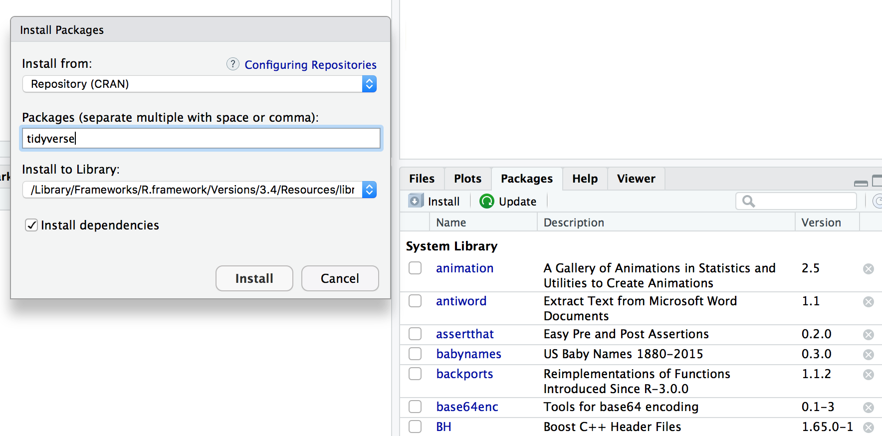
## Packages
To install the package `tidyverse` in RStudio go to the Packages tab in RStudio and click Install.
## Packages
- You’re not the only person writing your own functions with R.
- Many professors, programmers, and statisticians use R to design tools that can help people analyze data.
- They then make these tools free for anyone to use.
- To use these tools, you just have to download them. They come as preassembled collections of functions and objects called packages.
- We have already used two packages `ggplot2` and `dplyr`.
## Packages
To install the package `tidyverse` in RStudio go to the Packages tab in RStudio and click Install.
 To load a package type
```{r,eval=FALSE}
library(tidyverse)
```
## RStudio IDE
- IDE: Integrated Development Environment.
- The RStudio IDE has many features that we will not use in the course.
To load a package type
```{r,eval=FALSE}
library(tidyverse)
```
## RStudio IDE
- IDE: Integrated Development Environment.
- The RStudio IDE has many features that we will not use in the course.
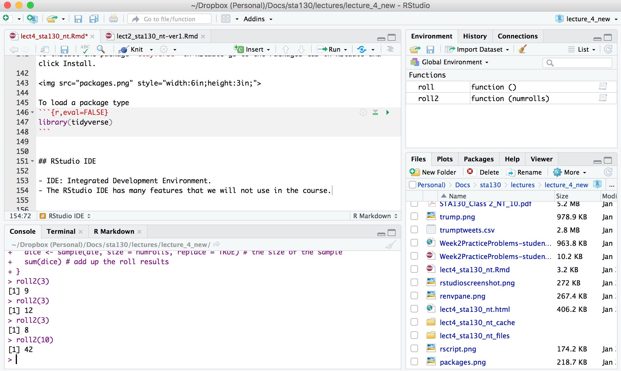 - The __console__ is where you can type an R command at the prompt and the result is returned.
- Write code in an R script, R Markdown document, or R Notebook.
- Run a script or R chunks from an R Markdown or R Notebook by pushing the run button in the chunk.
## R Objects
- R stores data in objects such as vectors, arrays, and matricies.
- In most applications we will ususally load data from an external file.
## R Objects - Atomic Vectors
You can make an atomic vector by grouping some values of data together with c:
```{r}
die<-c(1,2,3,4,5,6)
die
is.vector(die)
length(die)
```
## R Objects - Atomic Vectors
You can also make an atomic vector with just one value. R saves single values as an atomic vector of length 1:
```{r}
two <- 2
two
```
## R Objects - Atomic Vectors: Integer and Character
- Each atomic vector can only store one type of data. You can save different types of data in R by using different types of atomic vectors.
- R recognizes six basic types of atomic vectors: doubles, integers, characters, logicals, complex, and raw.
- We will not be using complex or raw types in STA130.
- Integer vectors included a capital L with input, and character vectors have input surounded by quotation marks.
## R Objects - Atomic Vectors: Integer and Character
```{r, error=TRUE}
mynums <- c(2L,3L)
courses <- "STA130"
courses <- c("STA130", "MAT137")
sum(mynums)
sum(courses)
sum(courses == "STA130")
```
## R Objects - Double Vectors
- A double vector stores real numbers. Doubles are often called numerics.
```{r}
die <- c(1,2,3,4,5,6)
typeof(die)
```
## R Objects - Logical Vectors
- Logical vectors store TRUEs and FALSEs, R’s form of Boolean data. Logicals are very helpful for doing things like comparisons:
```{r}
3 > 4
```
- TRUE or FALSE in capital letters (without quotation marks) will be treated as logical data. R also assumes that T and F are shorthand for TRUE and FALSE.
```{r}
logic <- c(TRUE, FALSE, TRUE)
logic
```
## R Objects - Atomic Vectors: `dim()`
You can transform an atomic vector into an n-dimensional array by giving it a dimen‐ sions attribute with dim.
```{r}
die <- c(1,2,3,4,5,6)
dim(die) <- c(2,3) # a 2x3 matrix
die
```
```{r}
die <- c(1,2,3,4,5,6)
dim(die) <- c(3,2) # a 3x2 matrix
die
```
R always fills up each matrix by columns, instead of by rows unless you use `matrix()` or `array()`.
## Factors
- Factors are R’s way of storing categorical information, like ethnicity or eye color.
- A factor as something like sex since it can only have certain values.
- Factors very useful for recording the treatment levels of a categorical variable.
```{r}
sex <- factor(c("male", "female", "female", "male"))
typeof(sex)
unclass(sex) # shows how R is storing the factor vector
```
## Coercion
R always follows the same rules when it coerces data types. Once you are familiar with these rules, you can use R’s coercion behavior to do surprisingly useful things.
- The __console__ is where you can type an R command at the prompt and the result is returned.
- Write code in an R script, R Markdown document, or R Notebook.
- Run a script or R chunks from an R Markdown or R Notebook by pushing the run button in the chunk.
## R Objects
- R stores data in objects such as vectors, arrays, and matricies.
- In most applications we will ususally load data from an external file.
## R Objects - Atomic Vectors
You can make an atomic vector by grouping some values of data together with c:
```{r}
die<-c(1,2,3,4,5,6)
die
is.vector(die)
length(die)
```
## R Objects - Atomic Vectors
You can also make an atomic vector with just one value. R saves single values as an atomic vector of length 1:
```{r}
two <- 2
two
```
## R Objects - Atomic Vectors: Integer and Character
- Each atomic vector can only store one type of data. You can save different types of data in R by using different types of atomic vectors.
- R recognizes six basic types of atomic vectors: doubles, integers, characters, logicals, complex, and raw.
- We will not be using complex or raw types in STA130.
- Integer vectors included a capital L with input, and character vectors have input surounded by quotation marks.
## R Objects - Atomic Vectors: Integer and Character
```{r, error=TRUE}
mynums <- c(2L,3L)
courses <- "STA130"
courses <- c("STA130", "MAT137")
sum(mynums)
sum(courses)
sum(courses == "STA130")
```
## R Objects - Double Vectors
- A double vector stores real numbers. Doubles are often called numerics.
```{r}
die <- c(1,2,3,4,5,6)
typeof(die)
```
## R Objects - Logical Vectors
- Logical vectors store TRUEs and FALSEs, R’s form of Boolean data. Logicals are very helpful for doing things like comparisons:
```{r}
3 > 4
```
- TRUE or FALSE in capital letters (without quotation marks) will be treated as logical data. R also assumes that T and F are shorthand for TRUE and FALSE.
```{r}
logic <- c(TRUE, FALSE, TRUE)
logic
```
## R Objects - Atomic Vectors: `dim()`
You can transform an atomic vector into an n-dimensional array by giving it a dimen‐ sions attribute with dim.
```{r}
die <- c(1,2,3,4,5,6)
dim(die) <- c(2,3) # a 2x3 matrix
die
```
```{r}
die <- c(1,2,3,4,5,6)
dim(die) <- c(3,2) # a 3x2 matrix
die
```
R always fills up each matrix by columns, instead of by rows unless you use `matrix()` or `array()`.
## Factors
- Factors are R’s way of storing categorical information, like ethnicity or eye color.
- A factor as something like sex since it can only have certain values.
- Factors very useful for recording the treatment levels of a categorical variable.
```{r}
sex <- factor(c("male", "female", "female", "male"))
typeof(sex)
unclass(sex) # shows how R is storing the factor vector
```
## Coercion
R always follows the same rules when it coerces data types. Once you are familiar with these rules, you can use R’s coercion behavior to do surprisingly useful things.
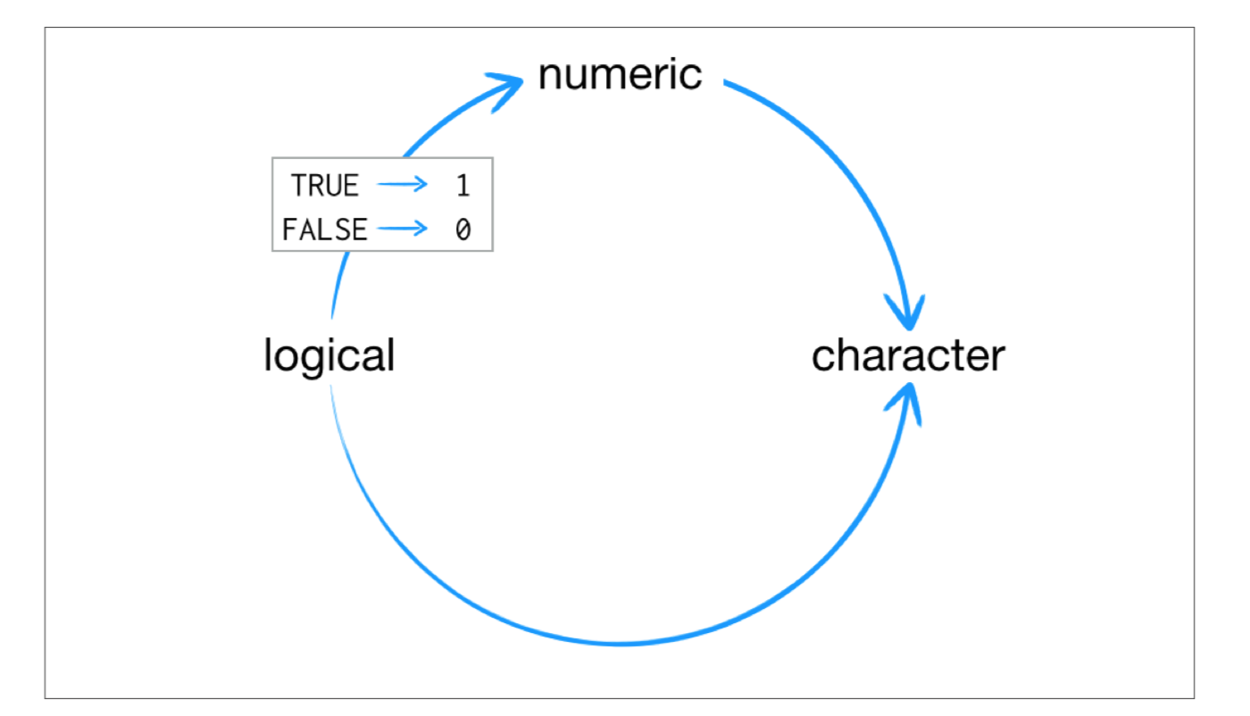 For example `sum(c(TRUE, TRUE, FALSE, FALSE))` will become `sum(c(1, 1, 0, 0))`.
```{r}
sum(c(TRUE, TRUE, FALSE, FALSE))
```
## Lists
- Lists are like atomic vectors because they group data into a one-dimensional set.
- Lists do not group together individual values.
- Lists group together R objects, such as atomic vectors and other lists.
- For example, you can make a list that contains a numeric vector of length 31 in its first element, a character vector of length 1 in its second element, and a new list of length 2 in its third element.
```{r}
list1 <- list(1:31, "Prof. Taback", list(TRUE, FALSE))
list1
```
## Data Frames
- Data frames are the two-dimensional version of a list.
- They are the most useful storage structure for data analysis
- A data frame is R’s equivalent to the Excel spreadsheet because it stores data in a similar format.
## Data Frames
- Data frames group vectors together into a two-dimensional table.
- Each vector becomes a column in the table.
- As a result, each column of a data frame can contain a different type of data; but within a column, every cell must be the same type of data.
For example `sum(c(TRUE, TRUE, FALSE, FALSE))` will become `sum(c(1, 1, 0, 0))`.
```{r}
sum(c(TRUE, TRUE, FALSE, FALSE))
```
## Lists
- Lists are like atomic vectors because they group data into a one-dimensional set.
- Lists do not group together individual values.
- Lists group together R objects, such as atomic vectors and other lists.
- For example, you can make a list that contains a numeric vector of length 31 in its first element, a character vector of length 1 in its second element, and a new list of length 2 in its third element.
```{r}
list1 <- list(1:31, "Prof. Taback", list(TRUE, FALSE))
list1
```
## Data Frames
- Data frames are the two-dimensional version of a list.
- They are the most useful storage structure for data analysis
- A data frame is R’s equivalent to the Excel spreadsheet because it stores data in a similar format.
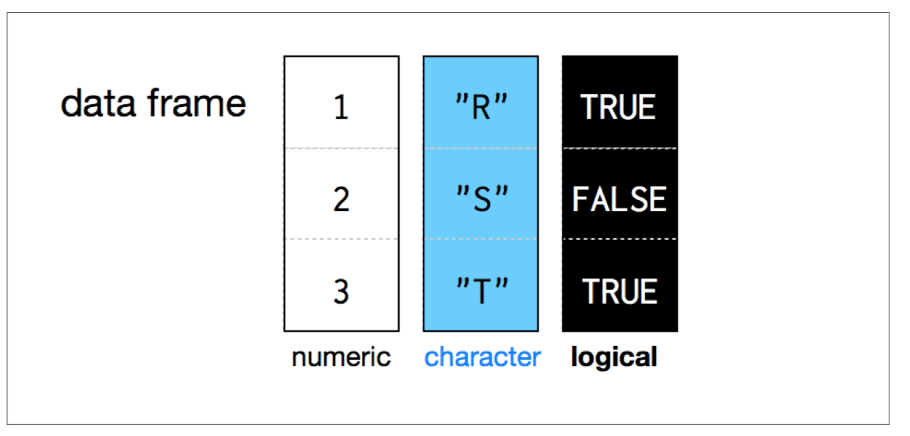
## Data Frames
- Data frames group vectors together into a two-dimensional table.
- Each vector becomes a column in the table.
- As a result, each column of a data frame can contain a different type of data; but within a column, every cell must be the same type of data.
 ## Data Frames
```{r,cache=TRUE}
student_num <- c(1, 2, 3, 4)
name <- c("Nadia", "Shiyi", "Yizhe", "Wei")
mydat <- data.frame(obsnum = student_num, student_name = name)
mydat
```
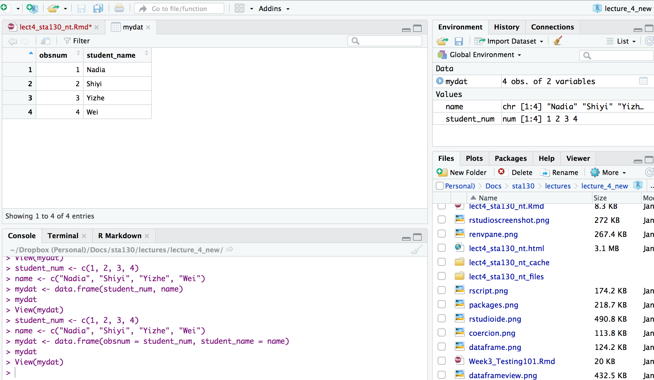
- Creating a data frame by hand takes a lot of typing, but you can do it with the `data.frame()` function.
- Give `data.frame()` any number of vectors, each separated with a comma.
- Each vector should be set equal to a name that describes the vector.
- `data.frame()` will turn each vector into a column of the new data frame.
## Data Frames
You can view a data frame in RStudio by clicking on the data frame name in the Environment tab
## Data Frames
```{r,cache=TRUE}
student_num <- c(1, 2, 3, 4)
name <- c("Nadia", "Shiyi", "Yizhe", "Wei")
mydat <- data.frame(obsnum = student_num, student_name = name)
mydat
```
- Creating a data frame by hand takes a lot of typing, but you can do it with the `data.frame()` function.
- Give `data.frame()` any number of vectors, each separated with a comma.
- Each vector should be set equal to a name that describes the vector.
- `data.frame()` will turn each vector into a column of the new data frame.
## Data Frames
You can view a data frame in RStudio by clicking on the data frame name in the Environment tab
 ## R Notation - [ , ]
- To extract a value or set of values from a data frame, write the data frame’s name followed by a pair of square brackets with a comma [ , ].
```{r, eval=FALSE}
mydat[ , ]
```
## R Notation - [ , ]
```{r}
mydat
mydat[1,2] # the value in row 1 and column 2
mydat[c(1,2),2] # all values in rows 1 and 2 in second column
```
## R Notation - $
The `$` tells R to return all of the values in a column as a vector.
```{r}
mydat$student_name
vec <- mydat$student_name # assign it to vec
attributes(vec) # info associated with object vec
vec[2] # get second element of vector
```
## R Notation - combine [,] and $
```{r}
mydat[mydat$obsnum == 1,] # first row of data frame and all columns
mydat[mydat$obsnum == 1 | mydat$obsnum == 4 ,] # first and fourth rows of data frame and all columns
```
## Missing Data - `NA`
- Missing information problems happen frequently in data science.
- For example a value is mising because the measurement was lost, corrupted, or never recorded.
- The `NA` character is a special symbol in R. It stands for “not available” and can be used as a placeholder for missing information.
```{r, error=TRUE}
1 + NA
```
## Missing Data - `na.rm()`
- Suppose you collected the ages of five students, but you forgot to record the fifth students age.
```{r, error=TRUE}
age <- c(19, 20, 17, 20, NA)
mean(age) # mean will be NA
```
```{r}
age <- c(19, 20, 17, 20, NA)
mean(age, na.rm = TRUE) # R will ignore missing values
```
## Identify and Set Missing Data - `is.na()`
```{r}
age <- c(19, 20, 17, 20, NA)
is.na(age) # check which elements of age are missing
age[1] <- NA # set the first element of age to NA
age
```
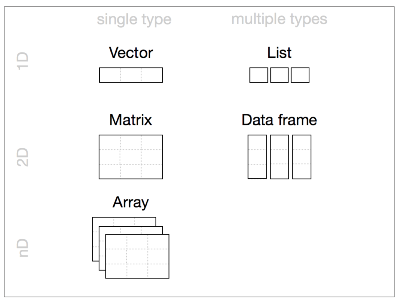
## Summary of R Data Structures
## R Notation - [ , ]
- To extract a value or set of values from a data frame, write the data frame’s name followed by a pair of square brackets with a comma [ , ].
```{r, eval=FALSE}
mydat[ , ]
```
## R Notation - [ , ]
```{r}
mydat
mydat[1,2] # the value in row 1 and column 2
mydat[c(1,2),2] # all values in rows 1 and 2 in second column
```
## R Notation - $
The `$` tells R to return all of the values in a column as a vector.
```{r}
mydat$student_name
vec <- mydat$student_name # assign it to vec
attributes(vec) # info associated with object vec
vec[2] # get second element of vector
```
## R Notation - combine [,] and $
```{r}
mydat[mydat$obsnum == 1,] # first row of data frame and all columns
mydat[mydat$obsnum == 1 | mydat$obsnum == 4 ,] # first and fourth rows of data frame and all columns
```
## Missing Data - `NA`
- Missing information problems happen frequently in data science.
- For example a value is mising because the measurement was lost, corrupted, or never recorded.
- The `NA` character is a special symbol in R. It stands for “not available” and can be used as a placeholder for missing information.
```{r, error=TRUE}
1 + NA
```
## Missing Data - `na.rm()`
- Suppose you collected the ages of five students, but you forgot to record the fifth students age.
```{r, error=TRUE}
age <- c(19, 20, 17, 20, NA)
mean(age) # mean will be NA
```
```{r}
age <- c(19, 20, 17, 20, NA)
mean(age, na.rm = TRUE) # R will ignore missing values
```
## Identify and Set Missing Data - `is.na()`
```{r}
age <- c(19, 20, 17, 20, NA)
is.na(age) # check which elements of age are missing
age[1] <- NA # set the first element of age to NA
age
```
## Summary of R Data Structures
 ## Tidyverse
 [https://www.tidyverse.org](https://www.tidyverse.org)
```{r,eval=TRUE, cache=TRUE, eval=TRUE, echo=FALSE}
# Uncomment next line if the rvest package is not installed
# install.packages("rvest")
library(rvest)
library(tidyverse)
url <- "https://www.canada.ca/en/public-health/services/surveillance/respiratory-virus-detections-canada/2017-2018/respiratory-virus-detections-isolations-week-1-ending-january-6-2018.html"
# download and read table into flu_dat
flu_dat <- url %>%
read_html() %>%
html_nodes(xpath = '/html/body/main/div[1]/div[2]/details[1]/table') %>%
html_table()
# clean up the file
fludat <- flu_dat[[1]]
dat <- as.data.frame(sapply(select(fludat,2:23), as.numeric))
fludat <- cbind(`Reporting Laboratory` = fludat[,1],dat)
fludat_prov <- fludat %>%
filter(row_number() < 42 & row_number() %in% c(1, 2, 3, 4, 12, 29, 30, 33, 34, 36, 37,38, 39)) %>%
select(prov = `Reporting Laboratory`, testpop_size = `Flu Tested`, fluA = `Total Flu A Positive`)
write_csv(fludat_prov,"fludat_prov.csv")
fludat_prov$prov <- recode(fludat_prov$prov, "Province of Québec" = "Quebec", "Province of Ontario" = "Ontario", "Province of Saskatchewan" = "Saskatchewan", "Province of Alberta" = "Alberta")
popurl <- "https://en.wikipedia.org/wiki/List_of_Canadian_provinces_and_territories_by_population_growth_rate"
popdat <- popurl %>%
read_html() %>%
html_nodes(xpath = '//*[@id="mw-content-text"]/div/table') %>%
html_table()
popdat <- popdat[[1]]
popdat <- popdat %>%
select(prov = `Province/Territory`, prov_pop_size = `2016 Census`) %>%
filter(row_number() < 14)
# remove comma and coerce to numeric
popdat$prov_pop_size <- as.numeric(gsub(",([[:digit:]])", "\\1", popdat$prov_pop_size))
popdat$prov[popdat$prov=="Newfoundland and Labrador"] <- "Newfoundland"
popdat$region <- c("Territories",NA,"West","Territories","West","West","East", NA,"Atlantic","Atlantic","Territories","Atlantic","Atlantic")
write_csv(popdat,"popdat.csv")
```
## Canadian Flu Rates with `dplyr`
The provincial rates for the week ending January 6, 2018 are in the file fludat_prov.csv and the the size of the population in each province is in the file popdat.csv. The code below reads the files into R data frames.
```{r, cache=TRUE}
library(tidyverse)
fludat_prov <- read_csv("fludat_prov.csv") # import data from file
popdat <- read_csv("popdat.csv") # import data from file
```
## Canadian Flu Rates with `dplyr`
```{r}
head(fludat_prov) # head shows the first six rows of a data frame
head(popdat)
```
## Canadian Flu Rates with `dplyr`
How many Provinces/Territories are in the fludat_prov data frame?
```{r}
fludat_prov %>% summarise(numprov = n()) # n() counts the number of rows in the data frame
```
## Canadian Flu Rates with `dplyr`
Do any variables in fludat or popdat have missing values?
```{r}
fludat_prov %>% filter(is.na(prov) == TRUE | is.na(testpop_size) == TRUE | is.na(fluA) == TRUE)
popdat %>% filter(is.na(prov) == TRUE | is.na(prov_pop_size) == TRUE | is.na(region) == TRUE)
```
## Canadian Flu Rates with `dplyr`
Recode specific values using R data frame notation [,] and $.
```{r}
popdat$region[popdat$prov == "Alberta"] <- "West" #recode only the region value for Alberta
popdat$region[popdat$prov == "Quebec"] <- "East" #recode only the region value for Alberta
popdat$region #print region variable in popdat data
```
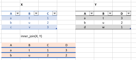
## Canadian Flu Rates with `dplyr` - Joining Two Tables with `inner_join()`
We can join two data frames with `inner_join(x,y)`: return all rows from x where there are matching values in y, and all columns from x and y. If there are multiple matches between x and y, all combination of the matches are returned.
```{r}
fludat_prov %>% inner_join(popdat, by = "prov")
```
Why are there only 9 observations when there are 13 Provinces/Territories?
## Canadian Flu Rates with `dplyr` - Joining Two Tables with `inner_join()`
```{r}
fludat_prov$prov
popdat$prov
```
Province needs to be recoded. Exercise on this week's practice problems.
## Canadian Flu Rates with `dplyr` - Joining Two Tables with `inner_join()`
[https://www.tidyverse.org](https://www.tidyverse.org)
```{r,eval=TRUE, cache=TRUE, eval=TRUE, echo=FALSE}
# Uncomment next line if the rvest package is not installed
# install.packages("rvest")
library(rvest)
library(tidyverse)
url <- "https://www.canada.ca/en/public-health/services/surveillance/respiratory-virus-detections-canada/2017-2018/respiratory-virus-detections-isolations-week-1-ending-january-6-2018.html"
# download and read table into flu_dat
flu_dat <- url %>%
read_html() %>%
html_nodes(xpath = '/html/body/main/div[1]/div[2]/details[1]/table') %>%
html_table()
# clean up the file
fludat <- flu_dat[[1]]
dat <- as.data.frame(sapply(select(fludat,2:23), as.numeric))
fludat <- cbind(`Reporting Laboratory` = fludat[,1],dat)
fludat_prov <- fludat %>%
filter(row_number() < 42 & row_number() %in% c(1, 2, 3, 4, 12, 29, 30, 33, 34, 36, 37,38, 39)) %>%
select(prov = `Reporting Laboratory`, testpop_size = `Flu Tested`, fluA = `Total Flu A Positive`)
write_csv(fludat_prov,"fludat_prov.csv")
fludat_prov$prov <- recode(fludat_prov$prov, "Province of Québec" = "Quebec", "Province of Ontario" = "Ontario", "Province of Saskatchewan" = "Saskatchewan", "Province of Alberta" = "Alberta")
popurl <- "https://en.wikipedia.org/wiki/List_of_Canadian_provinces_and_territories_by_population_growth_rate"
popdat <- popurl %>%
read_html() %>%
html_nodes(xpath = '//*[@id="mw-content-text"]/div/table') %>%
html_table()
popdat <- popdat[[1]]
popdat <- popdat %>%
select(prov = `Province/Territory`, prov_pop_size = `2016 Census`) %>%
filter(row_number() < 14)
# remove comma and coerce to numeric
popdat$prov_pop_size <- as.numeric(gsub(",([[:digit:]])", "\\1", popdat$prov_pop_size))
popdat$prov[popdat$prov=="Newfoundland and Labrador"] <- "Newfoundland"
popdat$region <- c("Territories",NA,"West","Territories","West","West","East", NA,"Atlantic","Atlantic","Territories","Atlantic","Atlantic")
write_csv(popdat,"popdat.csv")
```
## Canadian Flu Rates with `dplyr`
The provincial rates for the week ending January 6, 2018 are in the file fludat_prov.csv and the the size of the population in each province is in the file popdat.csv. The code below reads the files into R data frames.
```{r, cache=TRUE}
library(tidyverse)
fludat_prov <- read_csv("fludat_prov.csv") # import data from file
popdat <- read_csv("popdat.csv") # import data from file
```
## Canadian Flu Rates with `dplyr`
```{r}
head(fludat_prov) # head shows the first six rows of a data frame
head(popdat)
```
## Canadian Flu Rates with `dplyr`
How many Provinces/Territories are in the fludat_prov data frame?
```{r}
fludat_prov %>% summarise(numprov = n()) # n() counts the number of rows in the data frame
```
## Canadian Flu Rates with `dplyr`
Do any variables in fludat or popdat have missing values?
```{r}
fludat_prov %>% filter(is.na(prov) == TRUE | is.na(testpop_size) == TRUE | is.na(fluA) == TRUE)
popdat %>% filter(is.na(prov) == TRUE | is.na(prov_pop_size) == TRUE | is.na(region) == TRUE)
```
## Canadian Flu Rates with `dplyr`
Recode specific values using R data frame notation [,] and $.
```{r}
popdat$region[popdat$prov == "Alberta"] <- "West" #recode only the region value for Alberta
popdat$region[popdat$prov == "Quebec"] <- "East" #recode only the region value for Alberta
popdat$region #print region variable in popdat data
```
## Canadian Flu Rates with `dplyr` - Joining Two Tables with `inner_join()`
We can join two data frames with `inner_join(x,y)`: return all rows from x where there are matching values in y, and all columns from x and y. If there are multiple matches between x and y, all combination of the matches are returned.
```{r}
fludat_prov %>% inner_join(popdat, by = "prov")
```
Why are there only 9 observations when there are 13 Provinces/Territories?
## Canadian Flu Rates with `dplyr` - Joining Two Tables with `inner_join()`
```{r}
fludat_prov$prov
popdat$prov
```
Province needs to be recoded. Exercise on this week's practice problems.
## Canadian Flu Rates with `dplyr` - Joining Two Tables with `inner_join()`