---
title: "Running R"
---
## Running R online, 2025/2026 version
Go to [https://r.datatools.utoronto.ca](https://r.datatools.utoronto.ca):

Click Log In (the blue button) under R Studio.
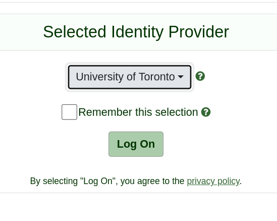
## Log in
{height="80%"}
Click Log On, to verify that you actually are at U of T.
## UTorID and password
{height="80%"}
as usual, but with *your* UTorID and password, not mine!
## After a moment...
... gets you to R Studio:
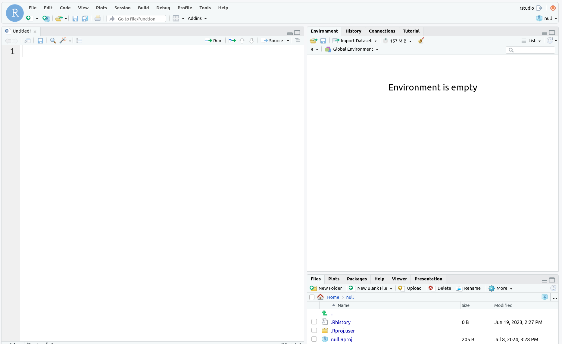
If already signed in with UTorID and password, you may get to skip some steps.
## Projects
- Each user has a “workspace”, a place where all your work is
stored.
- Within that workspace, you can have as many Projects as you like.
- I recommend having one project per *course*.
- R Studio restarts in project where you left off.
## Make a new project
- Call it what you like. Mine is called `thing`:
- Select:
- File,
- New Project,
- New Directory,
- New Project (again),
- give it a name and click Create Project.
- You see the name of your new project top right.
## Quarto documents
- At left of previous view is Console, where you can enter R commands
and see output.
- A better way to work is via “Quarto Documents”. These allow you to
combine narrative, code and output in one document.
- Data analysis is always a story: not only what you did, but why you
did it, with the “why” being more important.
- To create a new Quarto Document, select File, New File, Quarto Document. Give it a title. This
brings up an example document as over.
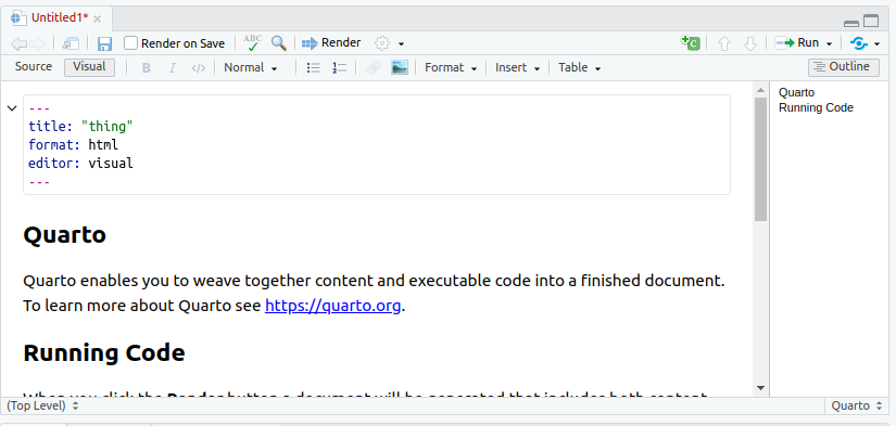
## The template document
{width=150%}
## About this document
- It begins with a title (that you can change).
- Most of the document is text (narrative).
- Pieces beginning with `{r}`, with grey background, are called code cells (code chunks). They
contain R code.
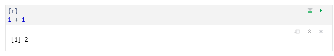
- Run code cells by clicking on the green “play button” at the top
right of the first cell. This one does some very exciting arithmetic.
## After running the code chunk
{width=150%}
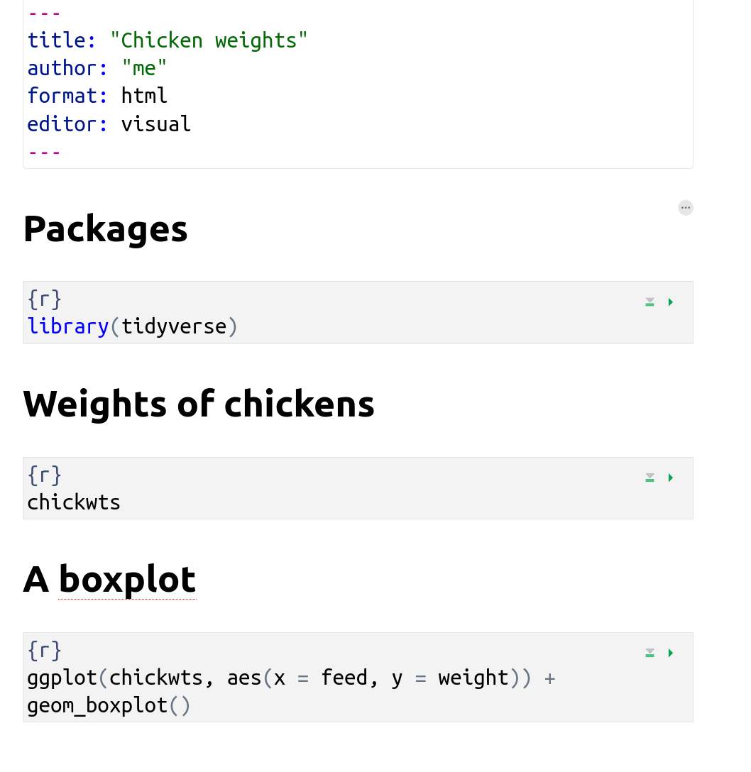
## Making our own document 1/2
- Create another new document. Give it a title of “Chicken weights by diet”, and click Create. When the document opens, delete the template that it gives you (leaving only the six lines that begin and end with `---`).
- Move the cursor to the next line below those top six lines.
- Type a `/` (slash). This allows you to insert something.
- Start typing "heading". When you see "Heading 2" in the list, select that.
- On this line, type **Packages** (which you'll see big and bold like a title) and hit Enter a couple of times. At the top of the window, you should now see Normal ( normal text).
## Making our own document 2/2
- Make a new code chunk: type a slash, then select the top option "R Code Chunk".
- Inside that cell, type
`library(tidyverse)`.
- Below that, make another "Heading 2" and put "Weights of chickens" on that line.
- Make another new code cell below that, and insert the line of
code: `chickwts`
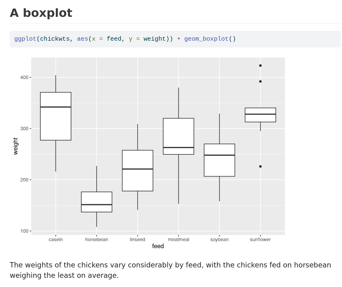
- Below that, make another Heading 2, "A boxplot", and another code cell containing
`ggplot(chickwts, aes(x = feed, y = weight)) + geom_boxplot()`.
## My document
{height="95%"}
## Run the chunks
- Now run each of the three chunks in order. You’ll see output below
each one, including a boxplot below the last one.
- When it works, add some narrative text before the code chunks
explaining what is going to be done, and some text after describing
what you see.
- Save the document (File, Save As). You don’t need a file extension.
- Click Render (at the top). This makes an HTML-formatted report, which may appear in another tab of your web browser.
- If you want to edit anything, go back to the Quarto document, change it,
save it, and run Render again. For example, you can try putting some of the text in *italics* or **bold**. (See Format.)
## The end of my (rendered) report
{height="90%"}
## Installing R on your own computer
- Free, open-source. Download and run on own computer.
- Three things:
- R itself (install first)
- R Studio (front end)
- Quarto (for writing reports).
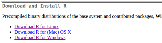
## Downloading R
- Go to .
- Click Download R (the link in the first paragraph) .
- R is stored on numerous “mirrors”, sites around the world. The top
one, “0-Cloud”, picks one for you.
{height="60%"}
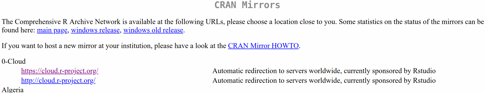
## Click your mirror
- Click 0-Cloud (or other mirror), get:
{width=150%}
- Click on your operating system, eg. Windows.
## Click on Base
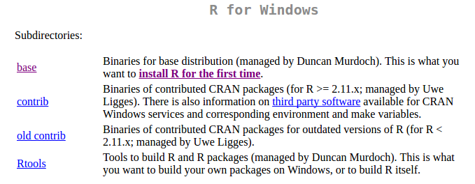{height="100%"}
- Click on “base” here.
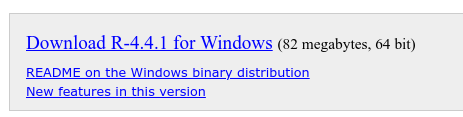
## The actual download
- The version number is, as I write this, 4.4.2, but there may be an update between me writing this and you reading it.
- For Windows, click something like the top link below (yours will have the latest version number):
## ... continued
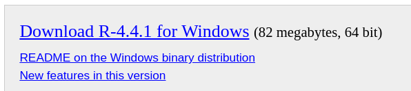
- Then install usual way.
- For Mac, install `R-4.4.1-arm64.pkg` (Big Sur with Apple Silicon M1-3), `R-4.4.1-x86_64.pkg` (Intel), or a newer version if available.
- Or, for Linux, click your distribution (eg. Ubuntu), then follow the instructions.
## Now, R Studio
- Go to . You will be redirected to `posit.co`, which is the new name of the company that makes R Studio.
- Click Open Source, then go down to Download R Studio (at the bottom).
- Scroll down to left Download R Studio button. Click it.
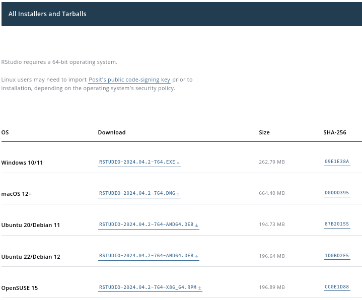
## Find the one for you
- We already installed R, so no need to do that.
- Scroll down to All Installers, and click the installer for your machine
(Windows, Mac, several flavours of Linux). Install as usual. See over.
## Choose the right one
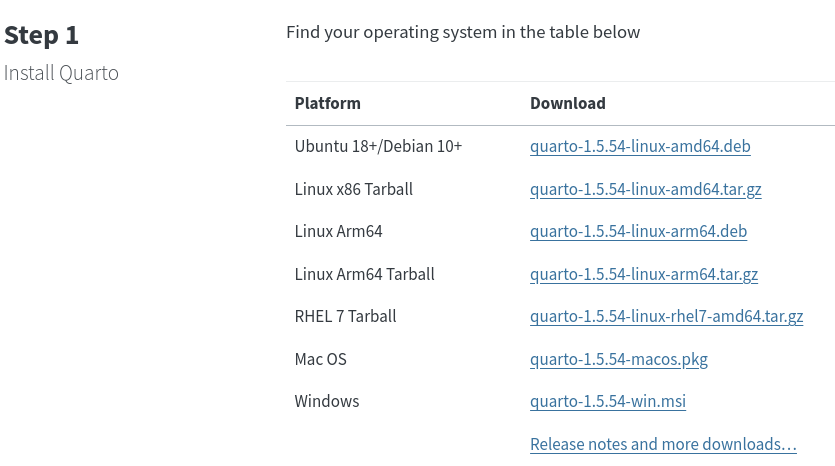
## Quarto
The last thing we need is Quarto, so that we can render documents (and thus hand in assignments).
- Go to .
- Click on one of the Get Started links (blue).
- Find your operating system and install as usual (over):
## Quarto 2/2
## Running R
- All of above only done once.
- To run R, run R Studio, which itself runs R.
## How R Studio looks when you run it
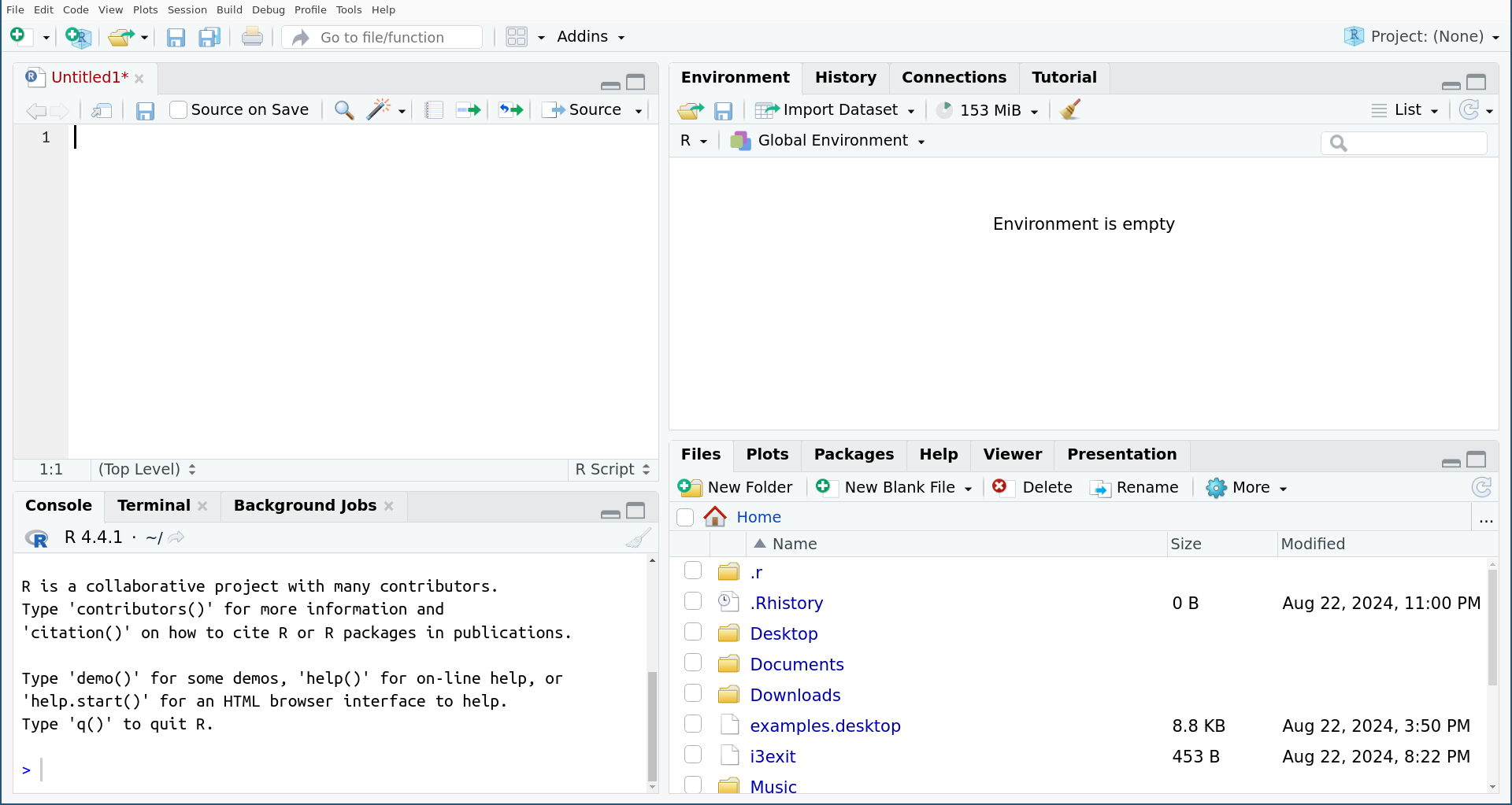{width=60%}
- that is, just the same as the online one.
## Install Tidyverse
- First time you run R Studio on your machine, click on Console window, and, next to the
`>`, type `install.packages("tidyverse")`. Let it do
what it needs to. (You need to do this on your machine. On `r.datatools.utoronto.ca`, it's already been done.)
## Projects
- A project is a “container” for code and data that belong together.
- Goes with a folder on some computer.
- File, New Project. You have option to create the new project in a
new folder, or in a folder that already exists.
- Use a project for a collection of work that belongs together, eg. data
files and Quarto documents for assignments. Putting everything in a project
folder makes it easier to find.
- Example: use a project for (all) assignments in a course, a different document
within that project for each one.