# Visualization
This article includes feature map visualization and Grad-Based and Grad-Free CAM visualization
## Feature map visualization
Visualization provides an intuitive explanation of the training and testing process of the deep learning model.
In MMYOLO, you can use the `Visualizer` provided in MMEngine for feature map visualization, which has the following features:
- Support basic drawing interfaces and feature map visualization.
- Support selecting different layers in the model to get the feature map. The display methods include `squeeze_mean`, `select_max`, and `topk`. Users can also customize the layout of the feature map display with `arrangement`.
### Feature map generation
You can use `demo/featmap_vis_demo.py` to get a quick view of the visualization results. To better understand all functions, we list all primary parameters and their features here as follows:
- `img`: the image to visualize. Can be either a single image file or a list of image file paths.
- `config`: the configuration file for the algorithm.
- `checkpoint`: the weight file of the corresponding algorithm.
- `--out-file`: the file path to save the obtained feature map on your device.
- `--device`: the hardware used for image inference. For example, `--device cuda:0` means use the first GPU, whereas `--device cpu` means use CPU.
- `--score-thr`: the confidence score threshold. Only bboxes whose confidence scores are higher than this threshold will be displayed.
- `--preview-model`: if there is a need to preview the model. This could make users understand the structure of the feature layer more straightforwardly.
- `--target-layers`: the specific layer to get the visualized feature map result.
- If there is only one parameter, the feature map of that specific layer will be visualized. For example, `--target-layers backbone` , `--target-layers neck` , `--target-layers backbone.stage4`, etc.
- If the parameter is a list, all feature maps of the corresponding layers will be visualized. For example, `--target-layers backbone.stage4 neck` means that the stage4 layer of the backbone and the three layers of the neck are output simultaneously, a total of four layers of feature maps.
- `--channel-reduction`: if needs to compress multiple channels into a single channel and then display it overlaid with the picture as the input tensor usually has multiple channels. Three parameters can be used here:
- `squeeze_mean`: The input channel C will be compressed into one channel using the mean function, and the output dimension becomes (1, H, W).
- `select_max`: Sum the input channel C in the spatial space, and the dimension becomes (C, ). Then select the channel with the largest value.
- `None`: Indicates that no compression is required. In this case, the `topk` feature maps with the highest activation degree can be selected to display through the `topk` parameter.
- `--topk`: only valid when the `channel_reduction` parameter is `None`. It selects the `topk` channels according to the activation degree and then displays it overlaid with the image. The display layout can be specified using the `--arrangement` parameter, which is an array of two numbers separated by space. For example, `--topk 5 --arrangement 2 3` means the five feature maps with the highest activation degree are displayed in `2 rows and 3 columns`. Similarly, `--topk 7 --arrangement 3 3` means the seven feature maps with the highest activation degree are displayed in `3 rows and 3 columns`.
- If `topk` is not -1, topk channels will be selected to display in order of the activation degree.
- If `topk` is -1, channel number C must be either 1 or 3 to indicate that the input data is a picture. Otherwise, an error will prompt the user to compress the channel with `channel_reduction`.
- Considering that the input feature map is usually very small, the function will upsample the feature map by default for easy visualization.
**Note: When the image and feature map scales are different, the `draw_featmap` function will automatically perform an upsampling alignment. If your image has an operation such as `Pad` in the preprocessing during the inference, the feature map obtained is processed with `Pad`, which may cause misalignment problems if you directly upsample the image.**
### Usage examples
Take the pre-trained YOLOv5-s model as an example. Please download the model weight file to the root directory.
```shell
cd mmyolo
wget https://download.openmmlab.com/mmyolo/v0/yolov5/yolov5_s-v61_syncbn_fast_8xb16-300e_coco/yolov5_s-v61_syncbn_fast_8xb16-300e_coco_20220918_084700-86e02187.pth
```
(1) Compress the multi-channel feature map into a single channel with `select_max` and display it. By extracting the output of the `backbone` layer for visualization, the feature maps of the three output layers in the `backbone` will be generated:
```shell
python demo/featmap_vis_demo.py demo/dog.jpg \
configs/yolov5/yolov5_s-v61_syncbn_fast_8xb16-300e_coco.py \
yolov5_s-v61_syncbn_fast_8xb16-300e_coco_20220918_084700-86e02187.pth \
--target-layers backbone \
--channel-reduction select_max
```
The above code has the problem that the image and the feature map need to be aligned. There are two solutions for this:
1. Change the post-process to simple `Resize` in the YOLOv5 configuration, which does not affect visualization.
2. Use the images after the pre-process stage instead of before the pre-process when visualizing.
**For simplicity purposes, we take the first solution in this demo. However, the second solution will be made in the future so that everyone can use it without extra modification on the configuration file**. More specifically, change the original `test_pipeline` with the version with Resize process only.
The original `test_pipeline` is:
```python
test_pipeline = [
dict(
type='LoadImageFromFile',
backend_args=_base_.backend_args),
dict(type='YOLOv5KeepRatioResize', scale=img_scale),
dict(
type='LetterResize',
scale=img_scale,
allow_scale_up=False,
pad_val=dict(img=114)),
dict(type='LoadAnnotations', with_bbox=True, _scope_='mmdet'),
dict(
type='mmdet.PackDetInputs',
meta_keys=('img_id', 'img_path', 'ori_shape', 'img_shape',
'scale_factor', 'pad_param'))
]
```
Change to the following version:
```python
test_pipeline = [
dict(
type='LoadImageFromFile',
backend_args=_base_.backend_args),
dict(type='mmdet.Resize', scale=img_scale, keep_ratio=False), # change the LetterResize to mmdet.Resize
dict(type='LoadAnnotations', with_bbox=True, _scope_='mmdet'),
dict(
type='mmdet.PackDetInputs',
meta_keys=('img_id', 'img_path', 'ori_shape', 'img_shape',
'scale_factor'))
]
```
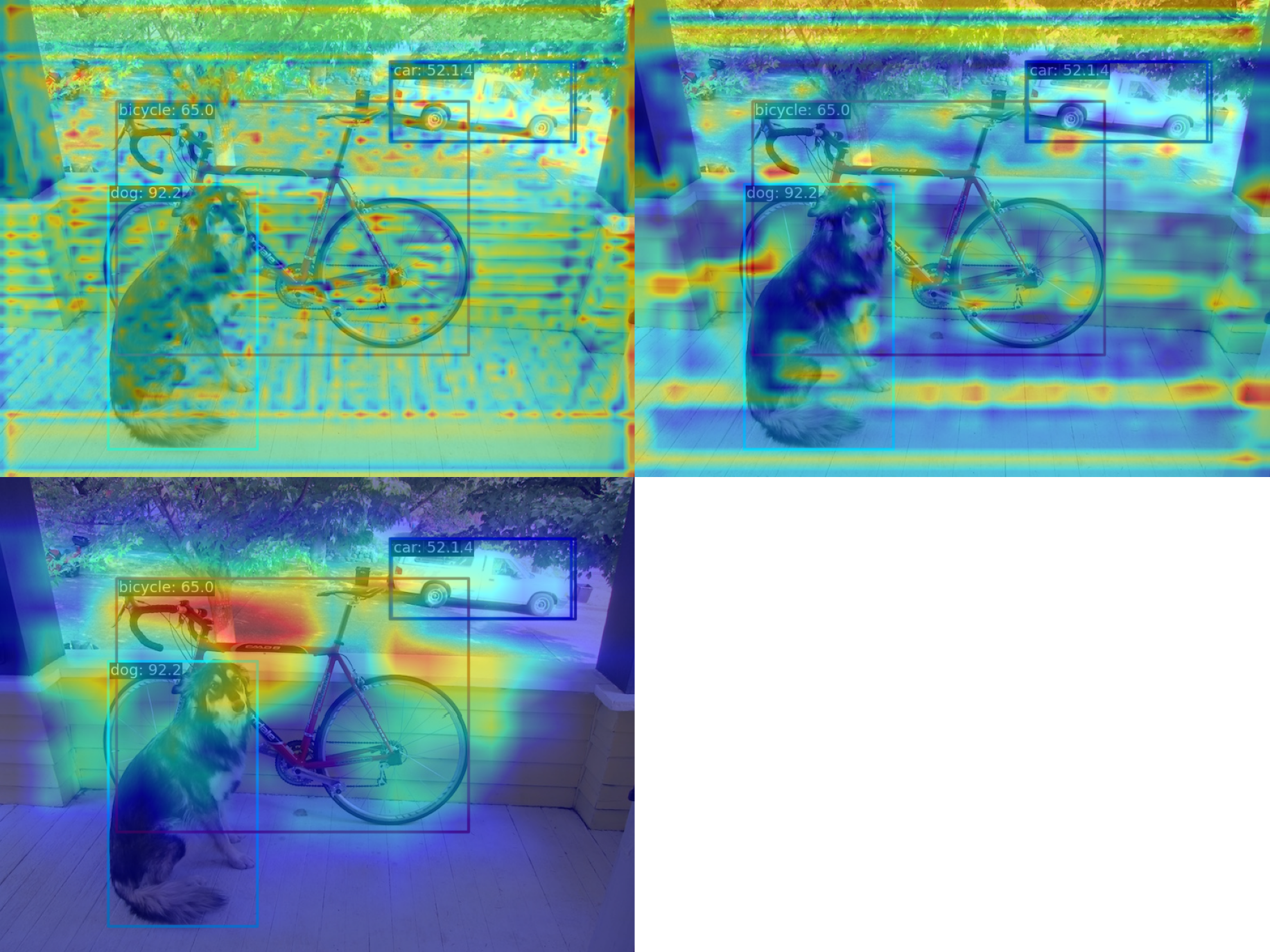
The correct result is shown as follows:
(2) Compress the multi-channel feature map into a single channel using the `squeeze_mean` parameter and display it. By extracting the output of the `neck` layer for visualization, the feature maps of the three output layers of `neck` will be generated:
```shell
python demo/featmap_vis_demo.py demo/dog.jpg \
configs/yolov5/yolov5_s-v61_syncbn_fast_8xb16-300e_coco.py \
yolov5_s-v61_syncbn_fast_8xb16-300e_coco_20220918_084700-86e02187.pth \
--target-layers neck \
--channel-reduction squeeze_mean
```
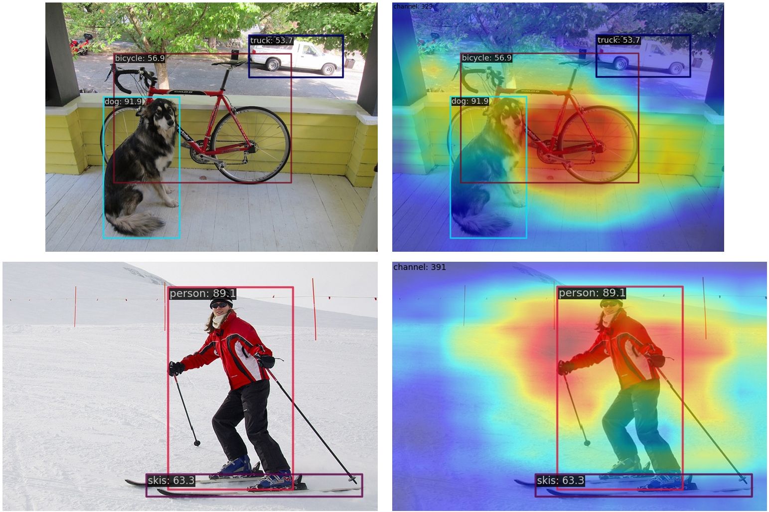
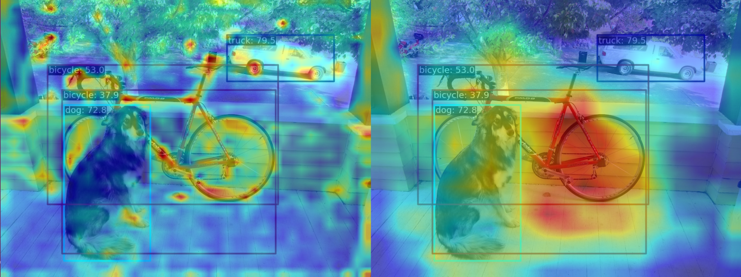
(3) Compress the multi-channel feature map into a single channel using the `squeeze_mean` parameter and display it. Then, visualize the feature map by extracting the outputs of the `backbone.stage4` and `backbone.stage3` layers, and the feature maps of the two output layers will be generated:
```shell
python demo/featmap_vis_demo.py demo/dog.jpg \
configs/yolov5/yolov5_s-v61_syncbn_fast_8xb16-300e_coco.py \
yolov5_s-v61_syncbn_fast_8xb16-300e_coco_20220918_084700-86e02187.pth \
--target-layers backbone.stage4 backbone.stage3 \
--channel-reduction squeeze_mean
```
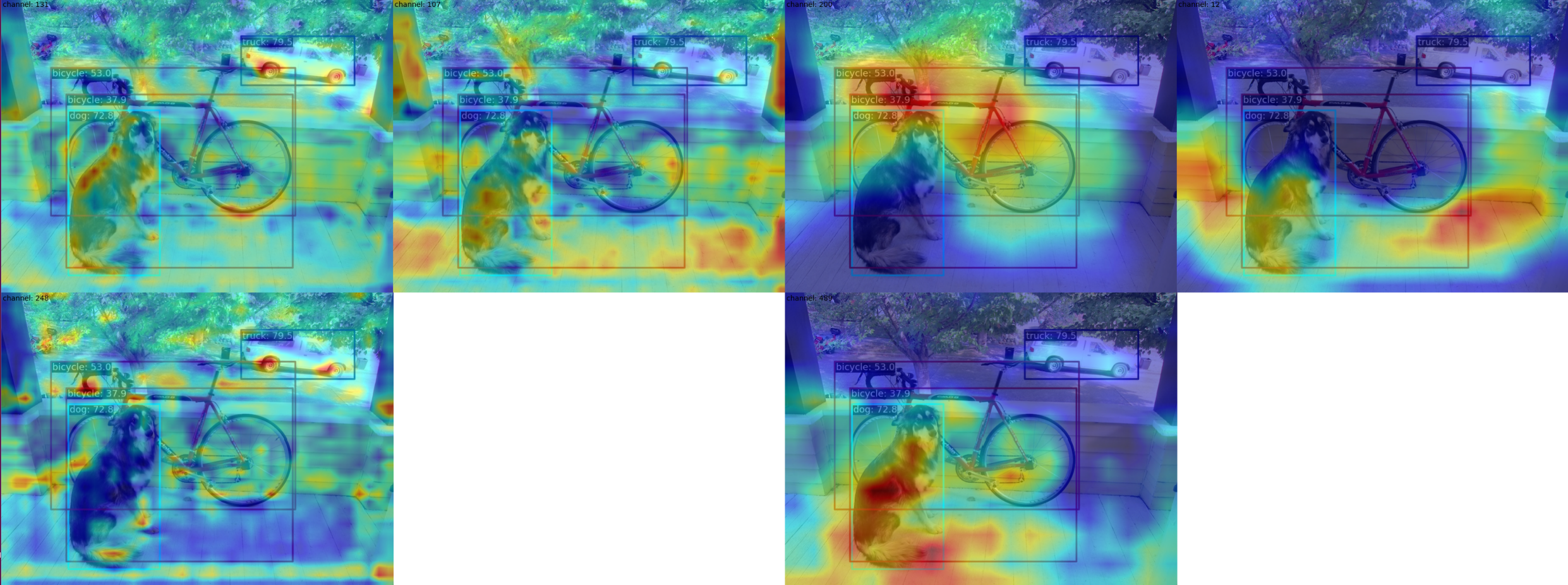
(4) Use the `--topk 3 --arrangement 2 2` parameter to select the top 3 channels with the highest activation degree in the multi-channel feature map and display them in a `2x2` layout. Users can change the layout to what they want through the `arrangement` parameter, and the feature map will be automatically formatted. First, the `top3` feature map in each layer is formatted in a `2x2` shape, and then each layer is formatted in `2x2` as well:
```shell
python demo/featmap_vis_demo.py demo/dog.jpg \
configs/yolov5/yolov5_s-v61_syncbn_fast_8xb16-300e_coco.py \
yolov5_s-v61_syncbn_fast_8xb16-300e_coco_20220918_084700-86e02187.pth \
--target-layers backbone.stage3 backbone.stage4 \
--channel-reduction None \
--topk 3 \
--arrangement 2 2
```
(5) When the visualization process finishes, you can choose to display the result or store it locally. You only need to add the parameter `--out-file xxx.jpg`:
```shell
python demo/featmap_vis_demo.py demo/dog.jpg \
configs/yolov5/yolov5_s-v61_syncbn_fast_8xb16-300e_coco.py \
yolov5_s-v61_syncbn_fast_8xb16-300e_coco_20220918_084700-86e02187.pth \
--target-layers backbone \
--channel-reduction select_max \
--out-file featmap_backbone.jpg
```
## Grad-Based and Grad-Free CAM Visualization
Object detection CAM visualization is much more complex and different than classification CAM.
This article only briefly explains the usage, and a separate document will be opened to describe the implementation principles and precautions in detail later.
You can call `demo/boxmap_vis_demo.py` to get the AM visualization results at the Box level easily and quickly. Currently, `YOLOv5/YOLOv6/YOLOX/RTMDet` is supported.
Taking YOLOv5 as an example, as with the feature map visualization, you need to modify the `test_pipeline` first, otherwise there will be a problem of misalignment between the feature map and the original image.
The original `test_pipeline` is:
```python
test_pipeline = [
dict(
type='LoadImageFromFile',
backend_args=_base_.backend_args),
dict(type='YOLOv5KeepRatioResize', scale=img_scale),
dict(
type='LetterResize',
scale=img_scale,
allow_scale_up=False,
pad_val=dict(img=114)),
dict(type='LoadAnnotations', with_bbox=True, _scope_='mmdet'),
dict(
type='mmdet.PackDetInputs',
meta_keys=('img_id', 'img_path', 'ori_shape', 'img_shape',
'scale_factor', 'pad_param'))
]
```
Change to the following version:
```python
test_pipeline = [
dict(
type='LoadImageFromFile',
backend_args=_base_.backend_args),
dict(type='mmdet.Resize', scale=img_scale, keep_ratio=False), # change the LetterResize to mmdet.Resize
dict(type='LoadAnnotations', with_bbox=True, _scope_='mmdet'),
dict(
type='mmdet.PackDetInputs',
meta_keys=('img_id', 'img_path', 'ori_shape', 'img_shape',
'scale_factor'))
]
```
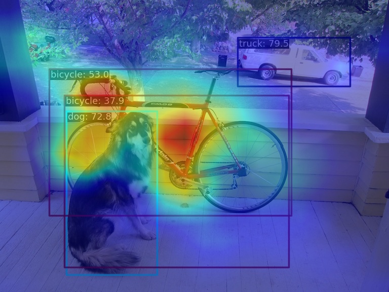
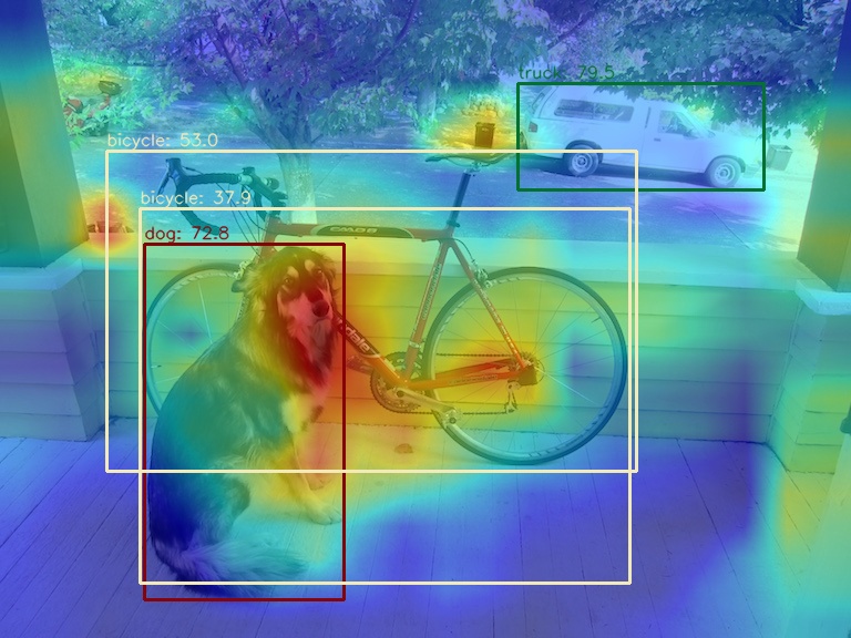
(1) Use the `GradCAM` method to visualize the AM of the last output layer of the neck module
```shell
python demo/boxam_vis_demo.py \
demo/dog.jpg \
configs/yolov5/yolov5_s-v61_syncbn_fast_8xb16-300e_coco.py \
yolov5_s-v61_syncbn_fast_8xb16-300e_coco_20220918_084700-86e02187.pth
```
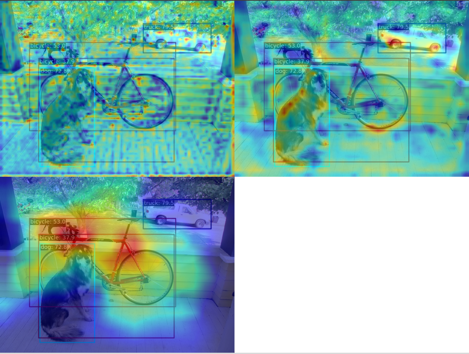
The corresponding feature AM is as follows:
It can be seen that the `GradCAM` effect can highlight the AM information at the box level.
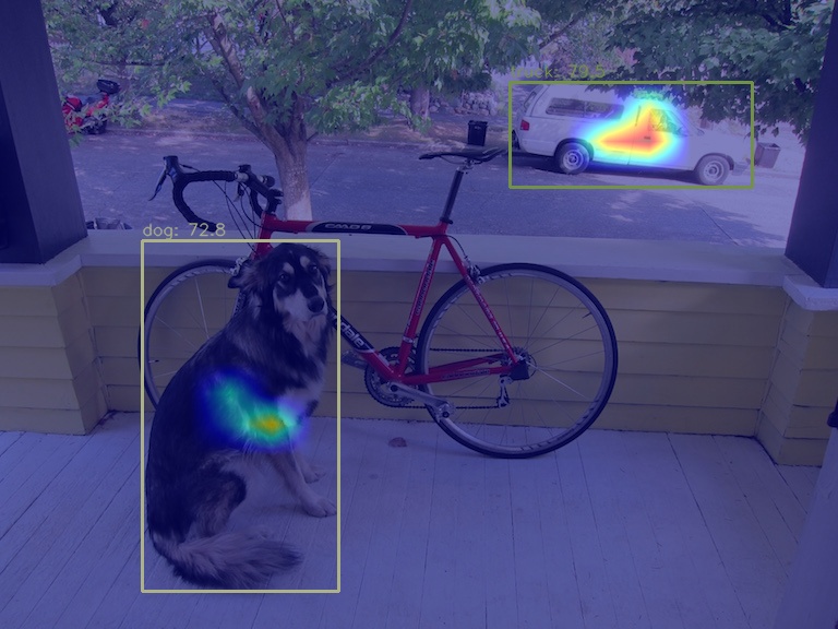
You can choose to visualize only the top prediction boxes with the highest prediction scores via the `--topk` parameter
```shell
python demo/boxam_vis_demo.py \
demo/dog.jpg \
configs/yolov5/yolov5_s-v61_syncbn_fast_8xb16-300e_coco.py \
yolov5_s-v61_syncbn_fast_8xb16-300e_coco_20220918_084700-86e02187.pth \
--topk 2
```
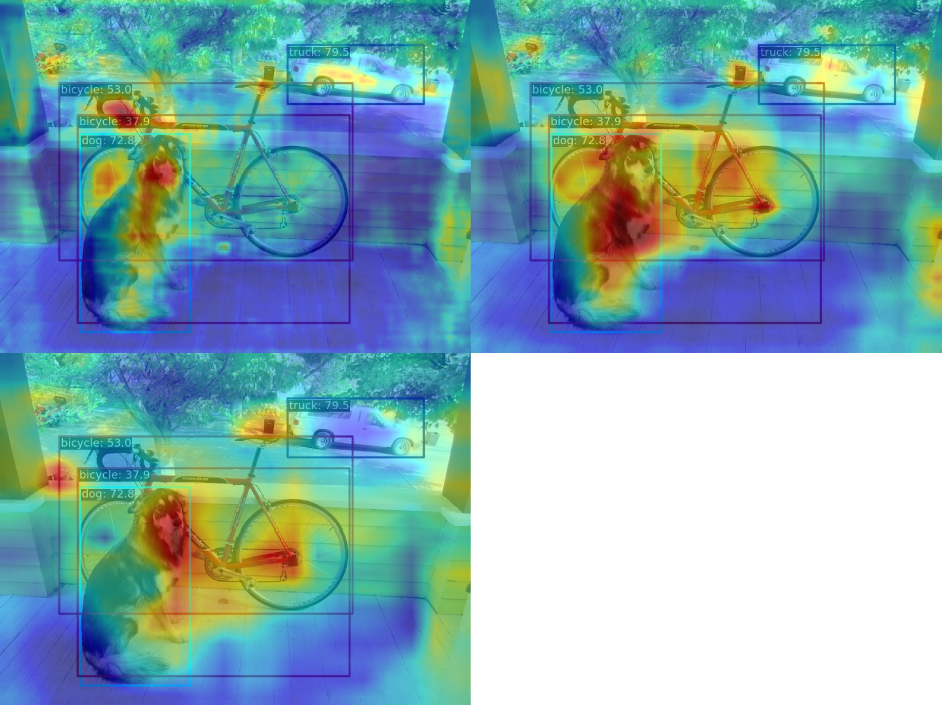
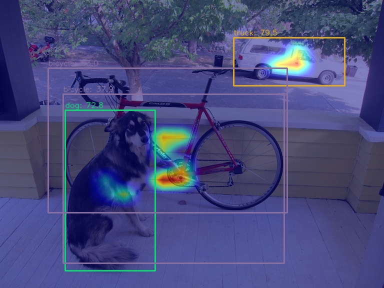
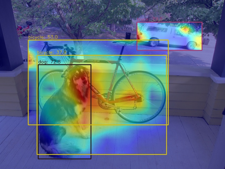
(2) Use the AblationCAM method to visualize the AM of the last output layer of the neck module
```shell
python demo/boxam_vis_demo.py \
demo/dog.jpg \
configs/yolov5/yolov5_s-v61_syncbn_fast_8xb16-300e_coco.py \
yolov5_s-v61_syncbn_fast_8xb16-300e_coco_20220918_084700-86e02187.pth \
--method ablationcam
```
Since `AblationCAM` is weighted by the contribution of each channel to the score, it is impossible to visualize only the AM information at the box level like `GradCAN`. But you can use `--norm-in-bbox` to only show bbox inside AM
```shell
python demo/boxam_vis_demo.py \
demo/dog.jpg \
configs/yolov5/yolov5_s-v61_syncbn_fast_8xb16-300e_coco.py \
yolov5_s-v61_syncbn_fast_8xb16-300e_coco_20220918_084700-86e02187.pth \
--method ablationcam \
--norm-in-bbox
```
## Perform inference on large images
First install [`sahi`](https://github.com/obss/sahi) with:
```shell
pip install -U sahi>=0.11.4
```
Perform MMYOLO inference on large images (as satellite imagery) as:
```shell
wget -P checkpoint https://download.openmmlab.com/mmyolo/v0/yolov5/yolov5_m-v61_syncbn_fast_8xb16-300e_coco/yolov5_m-v61_syncbn_fast_8xb16-300e_coco_20220917_204944-516a710f.pth
python demo/large_image_demo.py \
demo/large_image.jpg \
configs/yolov5/yolov5_m-v61_syncbn_fast_8xb16-300e_coco.py \
checkpoint/yolov5_m-v61_syncbn_fast_8xb16-300e_coco_20220917_204944-516a710f.pth \
```
Arrange slicing parameters as:
```shell
python demo/large_image_demo.py \
demo/large_image.jpg \
configs/yolov5/yolov5_m-v61_syncbn_fast_8xb16-300e_coco.py \
checkpoint/yolov5_m-v61_syncbn_fast_8xb16-300e_coco_20220917_204944-516a710f.pth \
--patch-size 512
--patch-overlap-ratio 0.25
```
Export debug visuals while performing inference on large images as:
```shell
python demo/large_image_demo.py \
demo/large_image.jpg \
configs/yolov5/yolov5_m-v61_syncbn_fast_8xb16-300e_coco.py \
checkpoint/yolov5_m-v61_syncbn_fast_8xb16-300e_coco_20220917_204944-516a710f.pth \
--debug
```
[`sahi`](https://github.com/obss/sahi) citation:
```
@article{akyon2022sahi,
title={Slicing Aided Hyper Inference and Fine-tuning for Small Object Detection},
author={Akyon, Fatih Cagatay and Altinuc, Sinan Onur and Temizel, Alptekin},
journal={2022 IEEE International Conference on Image Processing (ICIP)},
doi={10.1109/ICIP46576.2022.9897990},
pages={966-970},
year={2022}
}
```