# Analysis
## Selection and queries
**Home › Select** picks features by clicking or dragging a box. Open **Select options** to choose
**Select by Polygon** (click vertices; click the first vertex or double-click to finish), **Select by
Lasso** (drag a freehand outline), or **Select by Radius** (drag from the centre to set a distance). Shift adds to the
selection; Ctrl/Cmd removes; Esc cancels an unfinished outline. Area tools use even-odd fill, so a
self-crossing outline selects its alternating filled regions. Radius uses the Neighborhood Explorer's
local Mercator distance and retained geographic prefilter; its outline and readout are approximate
and some features near the outline may be excluded. A feature reaching beyond 85.05°, where Web
Mercator stops, is measured on the ground instead, so it may be selected outside the outline, which
stops at 85.05°, or left out inside it. The main Select button remains click/rectangle selection.
All selection tools take only features that are drawn, in selectable layers: a definition query or
a display filter hiding a feature keeps it out, and a click picks the feature drawn on top among the
selectable layers. **Select By Attributes** takes a SQL clause and checks it as you type; **Select By
Location** picks features that touch another layer's features or lie within a search distance of them (or,
inverted, those that don't). Selected features draw in
cyan and are highlighted in the attribute table, and the selection is synced both ways. Switch,
clear or zoom to the selection, or make a new layer from it (**Make Layer From Selected
Features**, `select.layerFromSelection`).
### The attribute table
++ctrl+t++ (or **Home › Selection › Attributes**) docks the active layer's table under the map.
Click a column header to sort by it (a second click reverses the order, a third unsorts), click a row to select it (++ctrl++ or
++shift++ toggles it without clearing the other rows), and double-click a cell to change its value. **Selected only**
keeps to the selected rows and **Filter rows…** keeps rows where any value contains the text typed,
ignoring letter case. The toolbar opens Select By Attributes and zooms to, switches, clears or
deletes the selection, adds or calculates a field, and calculates geometry attributes.
The first column, **Feature ID**, shows each feature's identifier, not its current row position
after sorting or filtering. It is not a dataset field: do not use it as a geoprocessing field name.
Right-click a column header for **Hide Column**, **Move Left**, **Move Right** and **Show All
Columns**. A hidden column is only left out of the table: export, selection, expressions and the
map are unchanged. The toolbar says how many columns are hidden, and clicking it shows them all.
Hiding the column the rows are sorted by clears the sort. The order and hidden columns are kept
per table until another project is opened, and are not saved in the project.
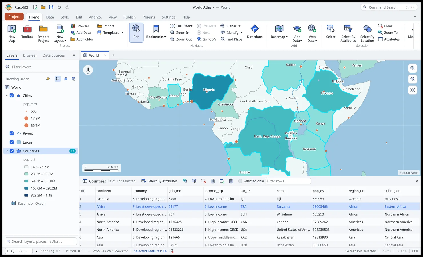
The attribute table, with a selection highlighted on the map and in the table.
Select By Attributes and definition queries use SQL `WHERE` clauses, written in the
[expression language](expressions.md):
```sql
pop_est > 100000000 AND continent = 'Asia'
name LIKE 'S%'
iso_a3 IN ('FRA', 'DEU', 'ITA')
gdp_md IS NULL
"OR" = 1 -- double quotes name a field, even a keyword
```
## Geoprocessing tools
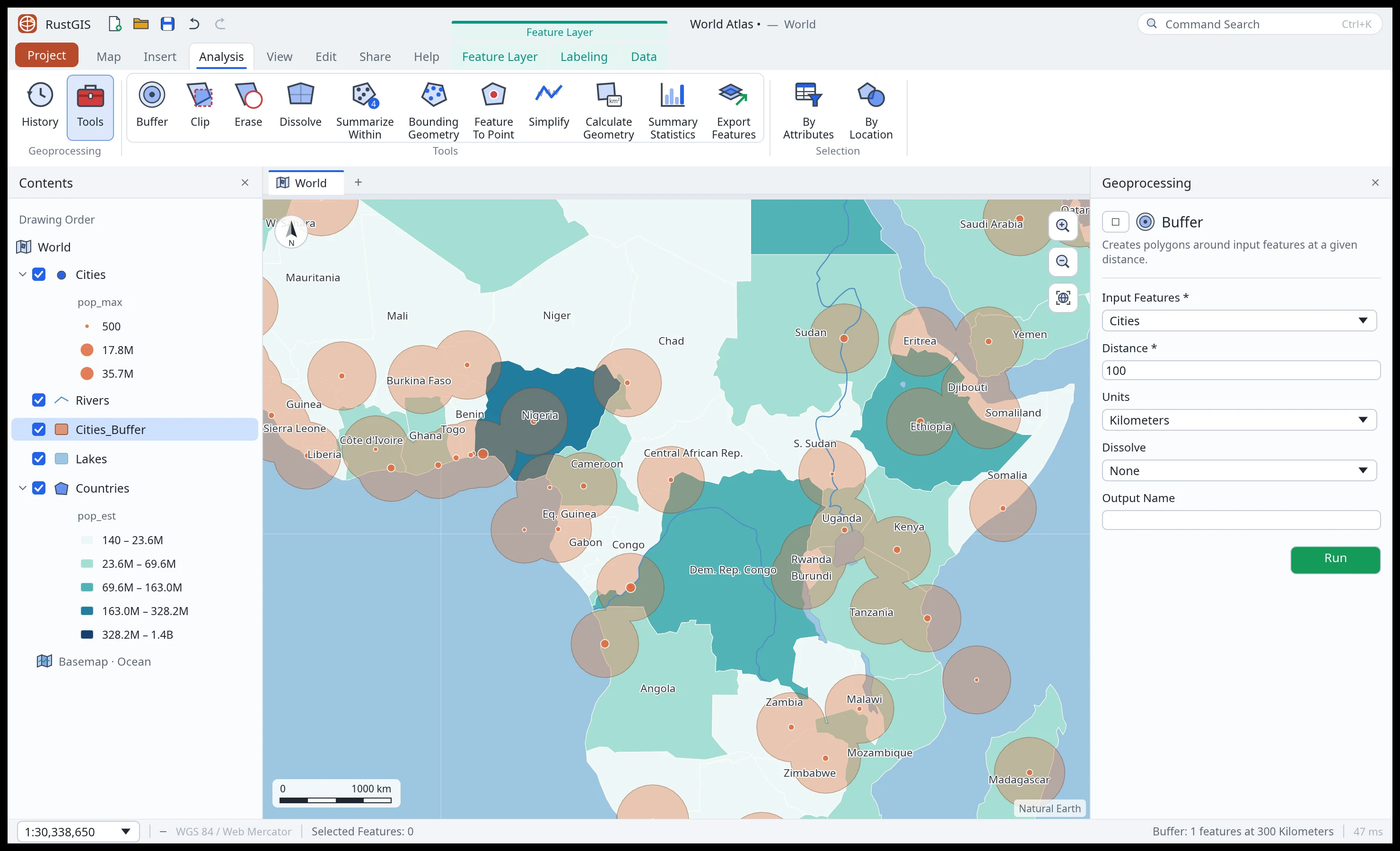
The Analyze tab's tool gallery and the Tools pane running Buffer.
Open a tool from **Analyze › Portal › Feature Analysis** or **Raster Analysis**, **Analyze › Tools** (the Tools pane,
which searches every tool) or Command Search. Fill in its parameters and click **Run**: new
layers or tables are added to the project; selection tools select existing rows and Calculate
Geometry Attributes updates the input layer. Each run is listed under **Analyze › History**.
In the desktop app a tool runs in the background, so the map and the rest of the window stay in
use. While it runs, the Tools pane shows its name, a **Cancel** button and, for the tools that
count their work (Viewshed, IDW Interpolation, Kriging, Kernel Density, Buffer, Select Layer By
Location and others), a progress bar. One tool runs at a time. A cancelled run adds nothing, and
for a tool that counts its work, its message says how far through its current step it got. Edits
made to its input layers while it runs are kept: a selection it makes selects the same features
where they now are (and says how many are gone), and a result that would replace an edited
layer, or one loaded whole meanwhile, is refused. Renaming the map while it runs is fine; after
switching to another map, a result that adds to or changes the map is refused (one made only of
tables or a file is still made). Opening another project drops the run. The Analysis pane's
**Zonal Statistics**, **Viewshed**, **Interpolate (IDW)**, **Suitability Modeler**, **Raster
Functions** and the **Function Editor**'s chains, **Change Detection**, **Classification Wizard**
(k-means), **Classification Tools** (from training polygons), **Indices**, **Process** (clip and resample), an ortho or
reality workspace's **Build** (its mosaic) and **Deep Learning** (training and classifying) run in
the background the same way, with their progress and **Cancel** under the pane's inputs, one at a
time; so does the map's right-click
**Viewshed … Here**, which opens the pane to show it. A model trained there is kept once its classes
are added: a cancelled run keeps none. Scripts, models, the AI
Assistant, the command line and the web app wait for each tool to finish.
**Viewshed**, **IDW Interpolation** and **Kriging** have no work limit when you run them from their
pane in the desktop app (the Tools or Analysis pane), nor does **Kernel Density** or **Deep
Learning**: a large run shows its progress, and **Cancel** stops it within a moment, however wide
its rows. Neither does `rustgis-cli run` typed at a terminal, which Ctrl-C stops. Where a run can't
be stopped while it goes (a script, a model, the AI Assistant, Python, the web app, and `rustgis-cli
run` called from another program, such as an agent or a CI job, which may wait with a timeout),
Viewshed, IDW Interpolation and Kriging refuse a run that would take more than a second or two of
work on one thread (a ray step, a cell-point pair), Kernel Density one whose points' search windows
(the square around each point's radius) cover more than 50 million cells, and Deep Learning a model
too large for its raster; its training fits a share of the sampled pixels, or fewer epochs, instead,
and says how many of each it trained on (`"limited"` in `dl.train`'s and `dl.classify`'s answer). A task or model recorded from a pane run keeps these limits
when it runs again in the app, so a step the pane took on can be refused there, and a model trained
again can differ. On the desktop these limits grow with the threads the run takes (the cores, up to 16 unless
[`threads`](#analysis-workflows) says otherwise), as many
times more work as the threads it runs on. Threads share cores and memory, so a run at that limit
can take up to about twice as long as a one-thread run at its own (measured on one machine, a Xeon
Silver 4114; it can be longer on others); in the web app, on one thread, the limits stay as they
are. The error names the limit on this computer and the threads it counted. The limits on memory
(the cells a grid may have, and those on the following pages) hold everywhere, as does Viewshed's on
its window: a radius covering more than 25 million cells, or 100,000 cells across, is refused. A
tool's own default cell size still follows the one-thread limit, so it makes the same grid on any
computer and from any caller; a finer cell size given is what a larger limit, or none, lets through.
From the command line or a script (`gp.run`), a built-in tool's parameter with a list of choices, such as Buffer's
units, takes one of them in any letter case (`"meters"` for `Meters`); any other value is an error
that names the choices (Buffer's units no longer take the abbreviations `m`, `mi` or `metres`).
Buffer and Select Layer By Location accept **Kilometers**, **Meters**, **Miles** and **Feet**. Feet are international feet
(exactly 0.3048 metres): a 500-foot notification radius is 152.4 metres on the ground.
The History pane lists each run with when it ran (in UTC). Its **⋯** menu, or a right-click on
the tool's name, copies a run as code, with the parameters it ran with: **Copy as Python** (a
call for the [`rustgis` package](../python.md), one parameter a line), **Copy as Command** (a
line for the Script pane) and **Copy as CLI Command** (`rustgis-cli run --project … --cmd …`,
quoted for a POSIX shell: macOS, Linux, WSL or Git Bash; on Windows' own shells, use the Python
or the Script line). **Open in Tool** opens the tool's form with those values, to change and run
again. **Save as Python Script…** writes the whole history as a script that opens the project
and runs each tool in order; a run that failed is there as a comment. The CLI command and the
script open the project's file: for a project not saved yet, they name the file it would be
saved as, so save it there first; and a project changed since it was saved needs saving again,
or the script opens it without those changes (a layer added since, say). What gives access is
taken out of the code: addresses lose their keys, tokens and passwords, a connection its
password, a pasted private key goes, and a parameter named as a password, key, secret or token
is left empty (`gp.historyCode` and `gp.historyScript` do the same from a script). A secret
written some other way (a token typed into a SQL query, say) can still be there: read the code
before sharing it. A point buffered where the
map was clicked is copied as the command that buffered it, with the point.
**Near the poles.** The geometry tools and the topology checks work on Web Mercator's coordinates,
carried on beyond 85.05°, where Web Mercator stops, to the poles instead of clamped there, so polar
features keep their shape. An edge wholly beyond 85.05° is straight in longitude and latitude. One
that crosses 85.05° is straight in the tools, but the Web Mercator map clamps its far end onto
85.05° and draws it straight to there, so a cut along such an edge can fall well east or west of
where that map shows it: about 48 km at 84.5°N for an edge from (0°, 80°N) to (10°E, 89°N). A
pole is a line in these coordinates, not a point, so Minimum Bounding Geometry of points spread
around a pole spans their longitudes (a flat polygon with no area, for points on one parallel,
and the tool says how many hulls have no area), not the cap they
enclose on the ground. The globe draws a long edge along the great circle between its ends, so near
a pole it shows a little poleward of where the tools take it: about 850 m at the middle of a 10°
edge along 88°N (as everywhere, the tools take an edge as straight on the map, not on the globe).
Beyond 85.05°, the dangle check measures line ends about their pole (on WGS 84's curvature there,
within 0.13% out to 85°), right up to the pole and across ±180°; an edge winding round a pole so
many times that it can't be measured closely is measured coarsely, and the check says it's
incomplete. Features that both reach a pole
(to within 1e-7°, about a centimeter) meet there, one place on the ground, in Select By Location
and Spatial Join (Intersects), whatever their longitudes; in Clip, the overlays, Erase, Split,
Summarize Within and Spatial Join ("Have their center in") a point at a pole falls in a polygon
reaching it (a line or polygon meeting another only at a pole has no part in it, as at a corner
anywhere); and a point at a pole is covered (Must Be Covered By) by polygons that together surround
the pole (elsewhere, a point on the boundary between two polygons is still reported, as before),
not by ones that only touch it at a corner or leave a gap reaching it (a hole no other polygon
fills included). The check looks at circles around the pole from 1.1 cm to 8.7 km from it on the
ground, out to the first the polygons don't reach at all: a gap more than 9e-6° of longitude wide
where it crosses one counts, and narrower ones are taken for the seams the overlays' rounding
leaves. It leans to reporting: such a gap counts even if it doesn't reach the pole, and so do
polygons reaching less far from the pole on one side than on another, within 8.7 km.
Spatial Join's Within, Contains and Largest overlap still see a pole as a line. Radius selections
and the Neighborhood Explorer measure a feature reaching beyond 85.05°, or any feature from a center
beyond it, on the ground, following each edge as the tools take it (straight on the map) to within
about 125 m out to 5,000 km (farther, more, but only ever nearer); the
Neighborhood Explorer also takes a center beyond 85.05°, while radius selections take centers within
±85.05°. A feature within ±85.05° searched from a center within it is still measured in local
Mercator, which doesn't go over the pole, so from a high latitude a feature just within 85.05° on
the far side of the pole can be left out while one just beyond it, nearer on the ground, is found.
A search measures at most 250,000 points and steps along edges in each layer, in steps of at most
half a degree; past them, or along an edge over 512° long (as only a hostile file has), a feature is
counted at the least distance it could be, so it may lie beyond the radius, and the tool warns how
many were, layer by layer. Shapes with a finite latitude past ±90° are left out of radius searches,
with a count; missing or infinite coordinates and their incident edges are omitted from the
measurement, also with a count. An incomplete polygon is measured along its remaining finite
edges, without assuming it contains the center. The overlay tools, Select By Location, Spatial Join, Summarize
Within and topology validation refuse latitudes past ±90° before doing their work.
### Batch geoprocessing (`gp.batch`)
Run one tool over many layers in the project or a folder of vector files:
```json
gp.batch={"tool":"buffer","inputs":["Cities","Rivers"],"outputPattern":"{input}_buf","params":{"distance":50,"units":"Kilometers"}}
```
- `"tool"`: the tool's id (such as `"buffer"`, `"simplify"` or `"convexHull"`).
- `"inputs"`: layer names or, on desktop and the command line, file paths; or `"*"` for every
vector layer on the active map, hidden ones included (raster and graphics layers are left out,
with a notice). In the browser, add a file as a layer first and use its layer name.
- `"folder"`: on desktop and the command line, a folder whose `.shp`, `.geojson`, `.json`,
`.gpkg`, `.fgb`, `.parquet`, `.geoparquet`, `.kml`, `.kmz`, `.gpx` and `.csv` files are run over
in file-name order (byte order, so ASCII capitals come before lowercase letters). Subfolders and symbolic links are skipped, with a count.
- `"outputPattern"` (or `"output_pattern"`): the name of each output layer, `"{input}_{tool}"` by
default, where `{input}` is the layer's name or the file's name without its extension and
`{tool}` the tool's id. It must include `{input}`. A name already taken gets a number (`_2`).
Tools that change a layer in place or select features keep their own names.
- `"params"`: the parameters every run shares. The batch input replaces a value given there for
the input parameter, with a notice.
- `"param"` (or `"batch_param"`): the parameter each input goes to; by default the tool's first
layer parameter, else `"input"`.
One input failing doesn't stop the others. The result counts what `"succeeded"` and `"failed"`,
names the `"outputs"` (layers or tables) and lists each failure in `"errors"`, with one notice
for the failures. If every input fails, the batch is an error naming each input and why. What a
reader drops or assumes for a file input (Z values, a coordinate system) is one notice per kind,
naming the inputs, and is kept in the history and the result's `"warnings"`. Tools that write a
file are refused. A batch is yours to run: the AI Assistant asks each time, and plugins and
imported tasks can't run one.
On the desktop, a batch in the Script pane runs in the background, as the script's tools do: the
status bar shows **Run Script** and **Cancel**. Cancel stops the batch after the item under way,
before the next one starts, and the run adds nothing. A batch run under a run that can be
cancelled stops with it, and says how many items it ran (`"cancelled"` and `"attempted"` in its
result, and a notice such as `Batch 'buffer' cancelled after 2 of 10`). On the command line,
Ctrl-C stops a batch as it stops any command.
### Built-in tools
These are the built-in tools; GeoLibre and plugin tools join them when available.
Use these ids in `gp.run`'s `tool` parameter (`gp.tools` lists the available tools and their parameters):
| Tool | Id | Toolbox |
| --- | --- | --- |
| Buffer | `buffer` | Analysis › Proximity |
| Near | `near` | Analysis › Proximity |
| Clip | `clip` | Analysis › Extract |
| Split | `split` | Analysis › Extract |
| Erase | `erase` | Analysis › Overlay |
| Intersect | `intersect` | Analysis › Overlay |
| Identity | `identity` | Analysis › Overlay |
| Union | `union` | Analysis › Overlay |
| Symmetrical Difference | `symmetricalDifference` | Analysis › Overlay |
| Update | `update` | Analysis › Overlay |
| Spatial Join | `spatialJoin` | Analysis › Overlay |
| Join Field | `joinField` | Data Management › Joins |
| Dissolve | `dissolve` | Data Management › Generalization |
| Minimum Bounding Geometry | `convexHull` | Data Management › Features |
| Feature To Point | `featureToPoint` | Data Management › Features |
| Merge | `merge` | Data Management › General |
| Feature Vertices To Points | `featureVerticesToPoints` | Data Management › Features |
| Points Along Lines | `pointsAlongLines` | Data Management › Features |
| Polygon To Line | `polygonToLine` | Data Management › Features |
| Split Line At Vertices | `splitLineAtVertices` | Data Management › Features |
| Feature Envelope To Polygon | `featureEnvelopeToPolygon` | Data Management › Features |
| Unsplit Line | `unsplitLine` | Data Management › Features |
| Check Geometry | `checkGeometry` | Data Management › Features |
| Repair Geometry | `repairGeometry` | Data Management › Features |
| XY Table To Point | `xyTableToPoint` | Data Management › Features |
| Calculate Geometry Attributes | `calculateGeometry` | Data Management › Features |
| Simplify | `simplify` | Cartography › Generalization |
| Tissot's Indicatrix | `tissot` | Cartography › Projections |
| A5 Grid | `a5Grid` | Analysis › DGGS |
| Aggregate Points to A5 | `a5Aggregate` | Analysis › DGGS |
| Select Layer By Location | `selectByLocation` | Data Management › Layers and Table Views |
| Select Layer By Attribute | `selectByAttributes` | Data Management › Layers and Table Views |
| Summarize Within | `countPoints` | Analysis › Summarize |
| Summary Statistics | `summaryStatistics` | Analysis › Statistics |
| Pivot Table | `pivotTable` | Analysis › Statistics |
| Tabulate Intersection | `tabulateIntersection` | Analysis › Statistics |
| Export Features | `exportFeatures` | Conversion |
| Vector to PMTiles | `vectorToPmtiles` | Analyze › Tools |
| Raster to PMTiles | `rasterToPmtiles` | Analyze › Tools |
| IDW Interpolation | `idwInterpolation` | Analysis › Interpolation |
| Ordinary Kriging | `kriging` | Analysis › Interpolation |
| Zonal Statistics | `zonalStats` | Analysis › Raster |
| Kernel Density | `kernelDensity` | Analysis › Density |
**Raster to PMTiles** (`rasterToPmtiles`) writes Web Mercator PNG tiles using the raster's current
bands, colors, mask and resampling. Set the minimum and maximum zoom from 0 to 16 and choose a
`.pmtiles` output; without one it uses the last component of the layer name. Layer and group
transparency are included. The raster must be georeferenced and fit
within one world. Turn off dynamic range adjustment and display rotation first. The in-memory
export is limited to 512 tiles and 64 MiB of compressed tile data; reduce the extent or zoom range
if it exceeds a limit. Areas beyond the Web Mercator latitude limit are clipped. A cloud-optimised
GeoTIFF read in place is exported from its full-resolution tiles: the desktop waits for them (two
minutes at most); the web app can't wait, so an export whose tiles aren't all in says so and asks
for the rest: export again once they are in (a large export may take a few tries). Without them
nothing is written.
**Vector to PMTiles** (`vectorToPmtiles`) writes a single-layer MVT archive in standard Web
Mercator. Choose `minZoom` and `maxZoom` from 0 to 16; `sourceLayer` defaults to the input
layer's name. The output file is saved atomically on desktop or downloaded in the browser.
Without `output`, CLI, script and task calls write `.pmtiles` in the process's working
directory, where `` is the layer's name without any folder part; an existing destination
is replaced atomically. The desktop tool pane instead asks for a destination with Save As.
Native exports refuse to replace the open/saved project file, the package this project was
opened from, or a file that a loaded layer, raster, standalone table or tile archive reads.
For directory-backed sources such as File Geodatabases, files inside the source directory are
protected as well.
This includes path aliases, ZIP archives holding loaded members, and Shapefile companion
files. Project/package paths stay anchored across changes to the working directory, and their
origins are restored when a project replacement is undone or redone. Browser downloads cannot
check the eventual save destination; choose a different file in the browser's save dialog to
avoid replacing an input.
An active selection is exported; otherwise the geoprocessing extent applies, and streamed
sources are read in full rather than limited to the visible map window. It exports points,
lines and polygons, including multipart geometry, attributes and feature IDs—not the map's
style or labels. Antimeridian paths are unwrapped and clipped with an 8/4096-tile buffer;
latitudes beyond Web Mercator's limit are clamped and reported. Geometry parts collapsed by
integer quantization and features without geometry are reported. Null properties are omitted;
integer attributes outside ±2^53 are rejected to avoid precision loss.
This is an in-memory export, limited to 10,000 distinct output tiles and a conservative
256 MiB working-memory budget, including the input, clipping/encoding temporaries and final
archive. This budget is checked after streamed-source materialization, not during provider
loading: the whole-read limits ([Large files](data.md#large-files)) apply first, and loading may
use more than 256 MiB before export refuses the input. Reduce a large source before loading it
for export. Geometry allocation estimates are linear in the number of vertices and rings.
Each geometry component's buffered candidate rectangle is limited to 40,000 tiles per zoom,
including candidates where clipping produces no output. A separate **100,000,000-unit
geometry-work budget** accumulates across all exported features, components and zooms:
each candidate tile costs the component's vertex count, and each polygon validity check
(before clipping and after integer quantization) costs `(vertices + rings)²`. The extra
vertex per ring allows for implicit ring closure. The work-limit error is distinct from
the memory-limit error: simplify polygon rings, reduce the input extent, or narrow the zoom
range. These limits reject the whole export rather than sampling or truncating it.
Browser task, model and script runs can queue at most eight files or 256 MiB of archive bytes
before downloads are submitted; split larger batches into separate runs. Browser success
means the download was submitted, not confirmation that the browser saved it. Example:
```text
gp.run={"tool":"vectorToPmtiles","params":{"input":"Roads","minZoom":0,"maxZoom":12,"sourceLayer":"roads","output":"roads.pmtiles"}}
```
**Simplify** uses Douglas–Peucker with a tolerance in kilometres. Each polygon ring keeps at
least three different, non-collinear corners (plus the closing vertex), so a tolerance larger
than a polygon produces a small ring instead of restoring its original vertices. Holes and
multipart rings are retained. This is not a topology-preserving simplifier: check the result
where holes or neighboring polygons must stay aligned. The default tolerance remains 25 km;
use a smaller value for local boundaries. A line or polygon has its tolerance taken east–west at
the scale of its middle (its label point's latitude), at most 85°'s, so beyond 85.05°, where the
ground is far narrower, less is simplified away than asked (a 3 km tolerance at 89.9°N takes out
only what lies within about 60 m east–west). Parts farther equatorward than the label point can be
simplified more than asked: the tolerance is applied at that one scale, so a polar cap from 60°N to
the pole, at 3 km, can move its 60°N vertices about 17 km on the ground. The tool says how many
features reach beyond 85.05° and so are affected.
**Kernel Density** (`kernelDensity`) calculates a continuous magnitude-per-unit-area raster
surface from point features using a Quartic (biweight, default) or Gaussian kernel (truncated at 3σ and
renormalised to integrate to 1).
Points can optionally be weighted by a numeric population field (invalid or non-positive weights
are excluded and reported in the tool messages; for multipoint features, each constituent point part
receives the feature's weight, a part with a coordinate missing or infinite is left out and
counted, and a feature with no finite part is skipped). Calculations are performed in the linear units
of a projected coordinate system (defaults to the layer's projected system; if the input layer lacks a
coordinate system or is in degrees, or to project into a specific system, supply a projected system via `crs`,
e.g. `EPSG:32618`).
Because bandwidth and cell size are measured in coordinate-space linear units, global cylindrical
projections such as Web Mercator (EPSG:3857) introduce scale distortion that increases with latitude;
use a local projected coordinate system (such as UTM or State Plane) when accurate ground distances
are required. A point the system can't hold, such as one beyond 85.05° in Web Mercator, is left
out, and the tool says how many were. Leaving `radius` empty or setting it to `0` automatically estimates the bandwidth
using Silverman's rule of thumb based on the points' spatial distribution (falling back to extent span / 30,
or 1000 coordinate-space linear units for a single point or coincident points). When `pixelSize` is
omitted, an adaptive cell size is calculated to span approximately 250 cells along the longer side
of the extent; the default search radius is automatically adjusted if needed to be at least the pixel
size so points are not missed between cell centres.
The search radius must be at least the pixel size. The extent can optionally be overridden via `extent`
as `xmin,ymin,xmax,ymax` text or a four-number array. The output is written as a single-band Float32 GeoTIFF.
Most feature tools process only the selected rows when an input has a selection. Selection tools
instead replace the input's selection; Select Layer By Location honours the selecting layer's
selection. Summarize Within counts the selected points against **all** input polygons, and
Calculate Geometry Attributes updates **all** rows. For tools that create a map layer, `output`
is the layer name; `vectorToPmtiles` uses it as a file destination.
**Buffer** distances, and the distance of **Select Layer By Location**, are measured on the Earth
(the WGS 84 ellipsoid, as PROJ and GeographicLib measure it), not in the map's display
projection. Each feature is buffered in an azimuthal equidistant projection on the ellipsoid
centred on it, so distances from a point are true; long lines and large polygon outlines are
buffered in stretches of a few hundred kilometres to limit projection error. Up to 85° of
latitude, a buffer's sides are within 0.012 % of the distance (or 1 cm), and within 0.05 % along
a winding line or outline buffered in stretches. An outline's edges are split to keep to that,
by at most 16,000 points a ring; a ring of thousands of long edges can use them up and keep some
edges coarser, and the tool says how many features' buffers did. Its curves are drawn with
straight edges (128 to a point's circle, 64 to a semicircular line end). Between vertices, those
edges cut up
to 0.031 % of the distance inside the true curve in the projection plane, and up to 0.125 % at
polygon corners and line joins, in addition to the projection error. Negative Buffer
distances shrink polygons. Buffer and Select Layer By Location limit distances to 5,000 km.
Ordinary Buffer limits each feature to 2,000,000 outline vertices. Its retained output has a
separate memory budget: on the desktop a quarter of the computer's memory, from 512 MiB up to 8 GiB
(`bufferBytes` in `gp.env`), and 128 MiB in the browser, including geometry
allocations, copied attributes and spare row capacity. Features are processed in bounded
batches, in input order. Many small buffers can therefore exceed 2,000,000 vertices together.
Dissolve All retains the shared 2,000,000-vertex limit before union and checks the dissolved
result too. Multipoint discs count before their union even when they overlap; for Dissolve All
their charges also accumulate across features.
Distance-based Select Layer By Location uses the same per-selector complexity limit and
memory budget for retained selector geometries, row capacity and a conservative spatial-index
storage allowance. With more than 16 distance selectors, selection stops with an error after
50,000,000 actual candidate checks across all target features, on both the grid and fallback
paths. Early matches stop their scan, so large input counts alone do not refuse a request.
Smaller selector sets keep their bounded-width linear scan. Selection at zero distance keeps
its existing behavior without these buffer limits. An excessive request fails with an error, never partial output; select fewer features
or split complex features. These budgets cover retained results, not total process memory:
the input layers, temporary geometry on active workers and polygon-overlay scratch are additional.
**Calculate Geometry Attributes** measures polygon areas and perimeters, and line lengths,
on the WGS 84 ellipsoid, independently of the map's display projection. Holes are subtracted
regardless of ring winding, and multipart measurements are summed. Ring directions are
normalized in continuous longitude space, so non-polar regions larger than half the Earth
keep their full area and small antimeridian crossings stay small. Rings winding around a pole
use the smaller polar region in either direction; reversing a ring does not select its global
complement. Edges follow the shortest geodesics between vertices. The output fields remain
`area_km2`, `perimeter_km` and `length_km`; point coordinates are unchanged.
A ring through both poles can wind beyond one whole surface and bound no single
region. Calculate Geometry Attributes refuses such input, with the numbers of affected rings
and features, before changing any fields. The attribute table's Calculate Geometry does the
same for its chosen rows. Spatial Join's Largest overlap refuses affected selected target or
join features before writing output. Ordinary polar caps and whole-world rectangles remain
measurable. Measure Area explains the ambiguity and still shows the perimeter.
Spatial Join's **Largest overlap** still measures area on a sphere of radius 6,371 km; it can
differ from the ellipsoid by up to about 0.9 % (a small area near a pole). The same WGS 84
measure backs the attribute table's **Calculate Geometry** (`edit.calculateGeometry`), the
[expressions](expressions.md#values)' `$area`, `$perimeter` and `$length`, the map's
**Measure** tools on the Earth, and every network tool's edge and route lengths, so all of these
read the same number for the same geometry, with one exception. A polygon ring with a full-turn
edge (-180° to 180° along a parallel that the ring reaches down one meridian and leaves back up
the other, with the ring's turns leaving it closed around the globe), such as a globe-wide band, is
measured along its parallels and meridians on the ellipsoid by all of them, its perimeter counting
each whole parallel; a 180° to -180° edge anywhere else is a seam along the antimeridian (a
polygon split there), measured as the meridian it runs along. A ring winding around a pole is
measured as the region it traces by the attribute table
and the Measure tools (a ring that goes all the way round at 60° N gives the larger region),
while **Calculate Geometry Attributes** gives the smaller polar cap. On the Moon or another body, the Measure tools measure on
that body's sphere. The Radius tools still measure a local Mercator distance, and **Mensuration
Tools** (`raster.measure`) still measure on the sphere, so those can differ from the numbers above.
For an ambiguous area, the `raster.measure` command with `kind: "area"` returns an error without a measurement object. To request its finite closed-ring perimeter, use `kind: "distance"` and repeat the first point at the end. The on-map Measure overlay continues to show perimeter alongside the area refusal.
**Merge** (`merge`, Data Management › General) appends loaded vector layers of the same geometry
type (points, lines or polygons) into a new layer. It needs no GeoLibre runner. Choose **Input
Layers** and **Preserve Attributes** in the tool pane, or pass names separated by `;` or a JSON
array. Desktop runs can also name local vector files without adding them to the map first.
In the browser, load the files as layers first. Each layer contributes its selection, or all its
features when it has no selection; read-in-place layers without a selection contribute their
complete source.
```json
{"tool":"merge","params":{"inputs":["Survey A","Survey B"],"attributes":true,"output":"Combined survey"}}
```
Matching field names (case-insensitive) and types share a column. Other fields are added and
missing values are empty. Incompatible types remain separate columns with unique suffixes,
such as `count_2`, preserving their original values and types. Turn off **Preserve Attributes**
for geometry only. Multipart geometry and holes are kept unchanged, new feature ids are assigned,
and export defaults to the first input's coordinate system; internal coordinates stay longitude
and latitude. The inputs stay unchanged, and the new layer can be undone.
**Feature Vertices To Points** (`featureVerticesToPoints`) writes a point at each vertex of the
`input` layer's features (a point layer's points are their own vertices, and a multipoint's points
its parts), with its feature's attributes and four fields. `orig_fid` is the feature's OID, linking
each point to its feature as ArcGIS's tool of the same name does. Three say where the point lies,
named as in QGIS's Extract Vertices: `vertex_part` (the part of a multipart feature),
`vertex_part_ring` (the polygon ring: 0 for the outer ring, and for lines and points) and
`vertex_part_index` (the place along the part or ring, from 0). Unlike QGIS's tool, it doesn't
write a polygon ring's closing point, which repeats its first. A new field whose name the input
already has gets a suffix (`vertex_part_2`). The points keep the input's coordinate system. In the
web app, the tool stops with a message if the browser can't give it the points' memory: select
fewer features, or simplify ones with many vertices.
```text
gp.run={"tool":"featureVerticesToPoints","params":{"input":"Rivers","output":"river_vertices"}}
```
**Points Along Lines** (`pointsAlongLines`) writes points at a set `distance` along each part of
the `input` layer's lines, or each ring of its polygons (holes too), measured on the WGS 84
ellipsoid as Buffer's distances are, in `units` (Kilometers by default): a point at `startOffset`
(0 by default), then one every `distance`, stopping `endOffset` before the part's end.
`includeEnd` adds a point where they stop when the distance doesn't land there (the first is
always at the start offset). Each part and ring is walked on its own from its first vertex, so the
gap between two parts never counts; a line's parts that cross the antimeridian, one ending on it
where the next begins on its other side, as a GeoJSON file splits a line that crosses it, are one
line. A ring ends where it starts, so a point there is made once, and a line that ends where it
starts (a contour) is walked as a ring too; a part shorter than its offsets gets none. A line that
passes through one place twice gets a point there each time the distance lands on it, except at a
closed line's shared start and end, which gets one point (a line through A, B and back to A gets
one at A). Each point
has its feature's attributes and three fields: `orig_fid`, the feature's OID, as Feature Vertices
To Points writes it, and, named as in QGIS's Points along geometry, `distance` (how far along its
part, in `units`, the start offset included) and `angle` (the line's direction there, in degrees
clockwise from north; on a vertex, halfway between the segments either side). A new field whose
name the input already has gets a suffix (`distance_2`). QGIS's tool works differently: it
measures `distance` along the whole feature (a polygon's rings as one, its end offset left out) in
the layer's units, and walks a closed line as an open one, which gets a point at its end, on its
start again, when the distance lands there. Here each part and ring starts again from 0, and the
distance is on the ground in any coordinate system. Missing geometry, point features, and line
or polygon features with no measurable segments (including empty geometries) are skipped with
separate counted notices. A valid part that produces no points because of the offsets is not
reported as unusable geometry.
Each edge is the shortest path between its vertices on the ellipsoid, as Calculate Geometry
Attributes measures it and the globe draws it. A flat map draws an edge straight in its own
projection instead (in Web Mercator, along a constant bearing), so a point on a long edge can sit
off the drawn line: on an east–west edge 100 km long, by about 200 m at 45° of latitude, 340 m at
60° and 1.1 km at 80° (on one 10 km long, a hundredth of that; on the equator or along a meridian,
not at all). Add vertices to long edges first if the points must follow the drawn line. An edge
spanning more than 180° of longitude is taken the short way round, and one from −180° to 180° at
one latitude has no length; a polygon cut at the antimeridian is walked as it is stored, so it gets
points along the cut too (a polar cap whose parallel is one edge from −180° to 180°, only along the
cut). An edge between opposite sides of the Earth has no single shortest path, and the tool takes
the one GeographicLib does (over a pole for two points on the equator).
The angle is the bearing from true north, which near a pole turns quickly along even a straight
line (by 33° in 30 m, 11 m from the North Pole); at a pole itself, where every direction is south,
it follows GeographicLib's convention, from the meridian of the longitude the vertex is written
with. On a map in another projection than Web Mercator, north isn't straight up everywhere, so
there the angle differs from the line's direction on the map. In Web Mercator it differs from a long
edge's drawn direction by about half the edge's span of longitude times the sine of the latitude:
at the ends of an east–west edge 100 km long, 0.45° at 45° and 2.5° at 80°; and, as Web Mercator
isn't conformal on the ellipsoid, from a diagonal edge's by up to about 0.19° at the equator (0.1°
at 45°, less toward the poles). A vertex less than a millimeter from the one before is passed over,
so a near-duplicate doesn't turn a point's angle; a vertex past a pole (bad data) is taken as the
pole, and the tool says how many it took so; and a vertex with a coordinate missing or infinite is passed over (its neighbors joined, or a
line's end trimmed back to the last vertex it has), and the tool says how many it passed over. The output keeps what the input lost on reading, if
anything (features, or Z and M values), as its layer's notes say. The points
keep the input's coordinate system, with longitudes between -180 and 180, so a point past the
antimeridian is on the far side of the map. The points are counted first and may take up to about
4 GiB (some 20 million points with a few fields): a distance that would make more, or more than
the browser can give in the web app, stops the tool with a message before anything is built. Use a
larger distance, simplify lines with very many vertices, or select fewer features.
```text
gp.run={"tool":"pointsAlongLines","params":{"input":"Rivers","distance":500,"units":"Meters","includeEnd":true}}
```
**IDW Interpolation** works like the QGIS tool of the same name: every point weighs on every
cell by 1/distanceᴾ, where P is the distance coefficient (2 by default). Lines and polygons
contribute their vertices. Leave the extent empty to use the input's, or give it as
`xmin,ymin,xmax,ymax`. `pixelSize` sets the cell size; when omitted it starts at 300 cells
across the extent and coarsens for large inputs. The result is a Float32 GeoTIFF layer. The
**Geostatistical Wizard** is a separate IDW workflow, with its coordinate system from Environments
(below): it uses 12 nearest neighbours by default (`neighbors`), rather than every point.
IDW Interpolation and Ordinary Kriging make their raster in the projected coordinate system given
as `crs` (such as `EPSG:32616` for UTM zone 16N, or a State Plane code), and then take the
extent, pixel size and Kriging's `range` in its units, usually metres or feet. Without `crs`
they work in longitude and latitude, with all three in degrees, as they did before `crs` was
there; for a layer read from a projected file they then say so, naming its system. A geographic
`crs` is refused, and points the system can't hold are left out and counted.
**Ordinary Kriging** (`kriging`) estimates both a value and its uncertainty. Set `input` and a
numeric `field`, then choose a `model`: **Spherical** (default), **Exponential** or **Gaussian**.
`neighbours` defaults to 12 (minimum 2, capped at 32). Optional `nugget`, `sill` and `range`
override the defaults: zero nugget, the sample variance (1 for near-constant values), and a
third of the extent's diagonal. `range`, `extent` and `pixelSize` are in the units of `crs`, or
in degrees without it (see above). Points at the same location are averaged; multipoints
contribute their points, while lines and polygons contribute their bounding-box centres. At least
two distinct locations with numeric values are needed. It adds **two separate Float32 GeoTIFF
layers**: the prediction, named by `output`, and `