---
title: "Lecture 8: Tidy data"
subtitle:  "EDUC 263: Managing and Manipulating Data Using R"
author:
date: 
urlcolor: blue
output: 
  html_document:
    toc: true
    toc_depth: 2
    toc_float: # toc_float option to float the table of contents to the left of the main document content. floating table of contents will always be visible even when the document is scrolled
      collapsed: false # collapsed (defaults to TRUE) controls whether the TOC appears with only the top-level (e.g., H2) headers. If collapsed initially, the TOC is automatically expanded inline when necessary
      smooth_scroll: true # smooth_scroll (defaults to TRUE) controls whether page scrolls are animated when TOC items are navigated to via mouse clicks
    number_sections: true
    fig_caption: true # ? this option doesn't seem to be working for figure inserted below outside of r code chunk    
    highlight: default # Supported styles include "default", "tango", "pygments", "kate", "monochrome", "espresso", "zenburn", and "haddock" (specify null to prevent syntax    
    theme: default # theme specifies the Bootstrap theme to use for the page. Valid themes include default, cerulean, journal, flatly, readable, spacelab, united, cosmo, lumen, paper, sandstone, simplex, and yeti.
    df_print: tibble #options: default, tibble, paged
    keep_md: true # may be helpful for storing on github
    
---

```{r, echo=FALSE, include=FALSE}
knitr::opts_chunk$set(collapse = TRUE, comment = "#>", highlight = TRUE)
  #comment = "#>" makes it so results from a code chunk start with "#>"; default is "##"
```

# Introduction

## Logistics

<br>

### Using `html_document` rather than `beamer_presentation` output for the next two lectures 

- What this means is that the lecture won't have "slides"; rather, I'll just scroll down
- Should be easier for you to "knit" entire lecture [Try it!] because doesn't rely on latex
- To see formatted version of lecture, open `lecture6.html` or knit and follow along in that version
- you will be able to run code chunks within .Rmd file as usual
- This is an experiment to see which you prefer; will inform revisions to next time I teach the class
- For Lectures 8, 9, and 10 we will go back to `beamer_presentation` with 

### Mid-term course survey

- A link to mid-term course survey will be posted at beginning of lecture 6 problem set. It is short. please complete it!
- focus is on how class is working for you; what is going well; how can class be improved

### Reading to do before next class

- Work through slides we from lecture 8 that we don't get to in class
    - [REQUIRED] slides from section "Tidying data"
    - [OPTIONAL] slides from section "Missing data"
- [REQUIRED] R developer blog on Pivoting
    - [LINK](https://tidyr.tidyverse.org/dev/articles/pivot.html#many-variables-in-column-names)
- [OPTIONAL] GW chapter 12 (tidy data)
    - Lecture covers this material pretty closely
    - Chapter functions for tidying data are limiting and outdated: `gather()` and `spread()`
- [OPTIONAL] Wickham, H. (2014). Tidy Data. _Journal of Statistical Software_, 59(10), 1-23. doi:10.18637/jss.v059.i10
    - This is the journal article that introduced the data concepts covered in GW chapter 12 and created the packages related to tidying data
    - Link to article here: [LINK](https://www.jstatsoft.org/article/view/v059i10)

### Libraries we will use today 

Functions we will use today are new and still under development, so you need to install the development version of tidyr
```{r}
#install.packages("devtools")
#devtools::install_github("tidyverse/tidyr")
```


You must run this R code chunk (install packages first if you don't have them)
```{r}
library(tidyverse)
library(haven)
library(labelled)
```



## Lecture overview

Creating analysis datasets often require __changing the organizational structure__ of data

Examples:

- You want analysis dataset to have one obs per student, but your data has one obs per student-course
- You want analysis dataset to have one obs per institution, but enrollment data has one obs per institution-enrollment level

Two common ways to change organizational structure of data

1. Use `group_by` to perform calculations separately within groups and then use `summarise` to create an object with one observation per group. Examples:
    - Creating objects containing summary statistics that are basis for tables and graphs (focus of lecture 4)
    - Creating student-transcript level GPA variable from student-transcript-course level data (focus of lecture 5 problem set)
1. __Reshape__ your data -- called __tidying__ in the R tidyverse world -- by transforming columns (variables) into rows (observations) and vice-versa
    - Our topic for today

This lecture is about changing the organizational structure of your data by transforming __untidy__ data into __tidy__ data.  

- Working with tidy data has many benefits, one of them is that all the packages in the tidyverse are designed to work with tidy data.
- We will perform data __tidying__ using functions from the __tidyr__ package, which is a package within tidyverse. 

Show index and example datasets in __tidyr__ package
```{r, eval=FALSE}
help(package="tidyr")

# note that example datasets table1, table2, etc. are listed in the index alongside functions
table1
tidyr::table1 # same same

df1 <- table1 # create an object from the "function" table1
str(df1)

table2
table3
```

# Data "structure" vs data "concepts"

Before we define "tidy data", we will spend significant time defining and discussing  some core terms/concepts about datasets. 

This discussion draws from the 2014 article [Tidy Data](https://www.jstatsoft.org/article/view/v059i10) by Hadley Wickham.

- Wickham (2014) distinguishes between "__data structure__" and "__data concepts__"
    - (Wickham actually uses the term "data semantics", but I don't know what the word "semantics" means, so I'll use the term "data concepts")


## Dataset structure

__Dataset structure__ refers to the "physical layout" of a dataset

- Typically, datasets are "rectangular __tables__ made up of __rows__ and __columns__" (emphasis added).
- a __cell__ is the intersection of one column and one row (think cells in Microsoft Excel)

There are many alternative data structures to present the same underlying data

- Below are two representations of the same underlying data that have different data structures (rows and columns transposed)

```{r}
#create structure a: treatment as columns, names as rows
structure_a <- tibble(
  name   = c("John Smith","Jane Doe","Mary Johnson"),
  treatmenta    = c(NA, 16, 3),
  treatmentb = c(2, 11, 1)
)

#create structure b: treatment as rows, names as columns
structure_b <- tibble(
  treatment   = c("treatmenta","treatmentb"),
  John_Smith    = c(NA, 2),
  Jane_Doe = c(16,11),
  Mary_Johnson = c(3,1)
)

structure_a
structure_b
```
### Unit of analysis

__unit of analysis__ [my term, not Wickham's]: 

- What each row represents in a dataset (referring to physical layout of dataset). 

Examples of different units of analysis:

- if each row represents a student, you have student level data
- if each row represents a student-course, you have student-course level data
- if each row represents an organization-year, you have organization-year level data
 
__Questions__: 

- What does each row represent in the data frame object `structure_a`?
```{r}
structure_a
```

- What does each row represent in the data frame object `structure_b`?
```{r}
structure_b
```

- What does each row represent in the data frame object `ipeds_hc_temp`?
    - Below we load data on 12-month enrollment headcount for 2015-16 academic year from the Integrated Postsecondary Education Data System (IPEDS)
```{r}
ipeds_hc_temp <- read_dta(file="https://github.com/ozanj/rclass/raw/master/data/ipeds/effy/ey15-16_hc.dta", encoding=NULL) %>% 
  select(unitid,lstudy,efytotlt) %>% arrange(unitid,lstudy)

ipeds_hc_temp
#show variable labels and value labels
ipeds_hc_temp %>% var_label()
ipeds_hc_temp %>% val_labels()

#print a few obs
ipeds_hc_temp %>% head(n=10)

#print a few obs, with value labels rather than variable values
ipeds_hc_temp %>% head(n=10) %>% as_factor()
```
### Which variable(s) uniquely identify rows in a data frame

Identifying which combination of variables uniquely identifies rows in a data frame helps you identify the "unit of analysis" and understand the "structure" of your dataset

- Said differently: for each value of this variable (or combination of variables), there is only one row
- Very important for reshaping/tidying data (this week) and very important for joining/merging data frames (next week)
- Sometimes a codebook will explicitly tell you which vars uniquely identify rows
- sometimes you have to figure this out through investigation
    - focus on ID variables and categorical variables that identify what each row represents; not continuous numeric variables like `total_enrollment` or `family_income`

__Task__: Let's try to identify the variable(s) that uniquely identify rows in `ipeds_hc_temp`

- Multiple ways of doing this
- I'll give you some code for one approach; just try to follow along and understand
```{r}
names(ipeds_hc_temp)
ipeds_hc_temp %>% head(n=10)
```

<br>
First, Let's investigate whether the ID variable `unitid` uniquely identifies rows in data frame `ipeds_hc_temp`

- I'll annotate code for each step
```{r}
ipeds_hc_temp %>% # start with data frame object ipeds_hc_temp
  group_by(unitid) %>% # group by unitid
  summarise(n_per_group=n()) %>% # create measure of number of obs per group
  ungroup %>% # ungroup (otherwise frequency table [next step] created) separately for each group (i.e., separate frequency table for each value of unitid)
  count(n_per_group) # frequency of number of observations per group
```

What does above output tell us?

- There are 5,127 values of `unitid` that have 2 rows for that value of `unitid`
- There are 1,824 values of `unitid` that have 3 rows for that value of `unitid`
- Note: `2*5127+3*1824==` `r format(round(2*5127+3*1824),nsmall=0, big.mark=",")` which is the number of observations in `ipeds_hc_temp`
- __Conclusion__: the variable `unitid` does not uniquely identify rows in the data frame `ipeds_hc_temp`

<br>
Second, Let's investigate whether the comination of `unitid` and `lstudy` uniquely identifies rows in data frame `ipeds_hc_temp`

```{r}
ipeds_hc_temp %>% # start with data frame object ipeds_hc_temp
  group_by(unitid,lstudy) %>% # group by unitid and lstudy
  summarise(n_per_group=n()) %>% # create measure of number of obs per group
  ungroup %>% # ungroup (otherwise frequency table [next step] created) separately for each group (i.e., separate frequency table for each value of unitid)
  count(n_per_group) # frequency of number of observations per group
```

What does above output tell us?

- There is `1` row each unique combination of `unitid` and `lstudy` 
- __Conclusion__: the variables `unitid` and `lstudy` uniquely identify rows in the data frame `ipeds_hc_temp`

What happens if we didn't ungroup?
```{r}
ipeds_hc_temp %>% # start with data frame object ipeds_hc_temp
  group_by(unitid,lstudy) %>% # group by unitid and lstudy
  summarise(n_per_group=n()) %>% # create measure of number of obs per group
  count(n_per_group) # frequency of number of observations per group
```

## Dataset (semantics) concepts

Think of these dataset _concepts_ as being distinct from dataset _structure_ (rows and columns)

<br>
The difference between data __structure__ and data __concepts__:

- Data __structure__ refers to the the physical layout of the data (e.g., what the rows and columns in a dataset actually represent)
- data __concepts__ -- which were introduced by Wickham (2014) -- refer to how the data __should__ be structured 

### Values, variables, and observations

Wickham (2014, p. 3): "A dataset is a collection of _values_, usually either numbers (if quantitative) or strings (if qualitative). Values are organized in two ways. Every value belongs to a _variable_ and an _observation_."

Wickham (2014) definitions of dataset concepts: _values_, _variables_, and _observations_ [I Recommend writing these definitions down on a separate sheet of paper]:

- __value__: A single element within some data structure (e.g., vector, list), usually a number or a character string.
    - e.g. the value of the variable `enrollment` for one organization in a dataset where each observation represents a postsecondary education institution
- __variables__: "A variable contains all values that measure the same underlying attribute (like height, temperature, duration) across units"
    - e.g., the variable `enrollment` is a vector that contains total enrollment for each organization in the dataset
- __observations__: "An observation contains all values measured on the same unit (like a person, or a day)...across attributes"
    - e.g., the values of each variable for one organization in a dataset where each observation represents a postsecondary education institution

Example of a dataset that satisfies Wickham definitions
```{r, echo=FALSE}
#Ignore this code; we'll explain it later in lecture
ipeds_hc_temp %>% 
  mutate(level = recode(as.integer(lstudy),
    `1` = "ug_enroll",
    `3` = "grad_enroll",
    `999` = "all_enroll")
  ) %>% select(-lstudy) %>% # drop variable lstudy
  spread(key = level, value = efytotlt) %>%
  select(unitid,ug_enroll,grad_enroll,all_enroll) %>%
  head(n=10)
```
<br>
Remove object
```{r}
rm(ipeds_hc_temp)
```

### Tables and observational unit

A particular project or data collection (e.g., longitudinal survey tracking student achievement from high school through college), may require several data sources:

- data on student characteristics (e.g., name, date of birth) with one observation per student
- data on the high school the student attends with one observation per school
- transcript data with one observation per student-course, etc.

Each of these data sources may use a different "level of observation" and each requiring a different "table" (i.e., dataframe):

- "Table" is the term database people use for what we would refer to as a "dataset" or a "data frame"
- We talk more about "tables" next week, which is about joining/merging data frames

<br>
__Observational unit/observational level__ [Wickham's term, not mine]

> "In a given analysis, there may be multiple __levels of observations__. For example, in a trial of new allergy medication we might have three observational types: demographic data collected from each person (age, sex, race), medical data collected from each person on each day (number of sneezes, redness of eyes), and meteorological data collected on each day (temperature,pollen count) (Wickham 2014, p. 4)"

<br>
So Wickham defines __observational unit/observational level__ as what each row __should__ represent in an appropriately structured data frame

### Summary/parting thoughts

These data concepts (e.g., value, variable, observation) seem easy on first glance, but can feel slippery on closer inspection. 

In particular, when you confronted with a particular dataset, sometimes it can feel confusing what the variables/observations/unit of analysis __are__ (data structure) and what they __should be__ (data concepts).

# Defining tidy vs. untidy data

## Rules of tidy data (defining tidy data)

Wickham chapter 12: "There are three interrelated rules which make a dataset tidy:

1. Each __variable__ must have its own __column__
1. Each __observation__ must have its own __row__
1. Each __value__ must have its own __cell__"
1. [Additional rule from Wickham (2014)] Each type of __observational unit__ forms a __table__

I Recommend writing these rules down on a separate sheet of paper

"These three rules are interrelated because it’s impossible to only satisfy two of the three" (Wickham chapter 12)

<br>
__Visual representation of the three rules of tidy data__:

![](http://r4ds.had.co.nz/images/tidy-1.png)
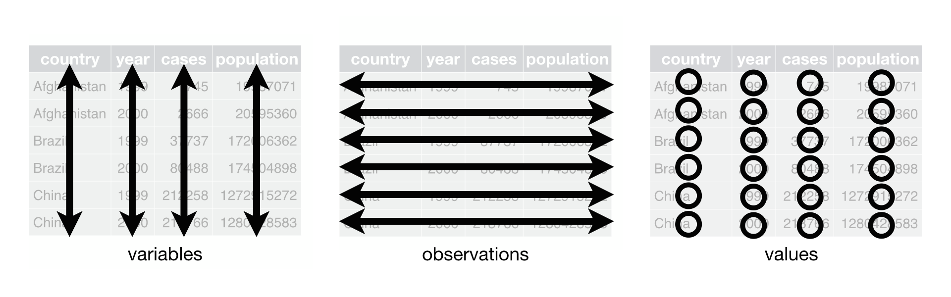
Here is an example of tidy data:
```{r}
#help(package="tidyr")
table1
```

Question: 

- What is does each observation (data concept) represent in the above dataset?
- What is does each row (data structure) represent in the above dataset?

## Untidy data

> “Tidy datasets are all alike, but every messy dataset is messy in its own way.” –– Hadley Wickham

While __all__ tidy datasets are organized the same way, untidy datasets can have several different organizational structures

<br>
Here is an example of an untidy version of the same data shown in `table1`
```{r}
#Untidy data, table 2
#help(package="tidyr")
table2
```

Other examples of untidy data (output omitted):
```{r, eval=FALSE}
table3

#tables 4a and 4b put the information from table1 in two separate data frames
table4a
table4b

table5
```

## Diagnosing untidy data

The first step in transforming untidy data to tidy data is diagnosing which principles of tidy data have been violated.

Recall the three principles of tidy data:

1. Each variable must have its own column.
1. Each observation must have its own row.
1. Each value must have its own cell.

Let's diagnose the problems with `table2` by answering these questions

1. Does each variable have its own column?
    - if not, how does the dataset violate this principle?
    - what _should_ the variables be?
1. Does each observation have its own row?
    - if not, how does the dataset violate this principle?
    - what does each row represent _actually_ represent?
    - what _should_ each row represent?
1. Does each value  have its own cell."
    - if not, how does the dataset violate this principle?
    
Printout of `table2`
```{r}
table2
```

Answers to these questions:

1. Does each variable have its own column? __No__
    - if not, how does the dataset violate this principle? __"cases" and "population" should be two different variables because they are different attributes, but in `table2` these two attributes are recorded in the column "type" and the associated value for each type is recorded in the column "count"__
    - what _should_ the variables be? __country, year, cases, population__
1. Does each observation have its own row? __No__
    - if not, how does the dataset violate this principle? __there is one observation for each country-year-type. But the values of type (population, cases) represent attributes of a unit, which should be represented by distinct variables rather than rows. So `table2` has two rows per observation but it should have one row per observation__
    - what does each row represent _actually_ represent? __country-year-type__
    - what _should_ each row represent? __country-year__
1. Does each value  have its own cell." __Yes__.
    - if not, how does the dataset violate this principle?

## Student exercise:

For each of the following datasets -- `table1`, `table3`, `table4a`, and `table5` -- answer the following questions:

1. Does each variable have its own column?
    - if not, how does the dataset violate this principle?
    - what _should_ the variables be?
1. Does each observation have its own row?
    - if not, how does the dataset violate this principle?
    - what does each row represent _actually_ represent?
    - what _should_ each row represent?
1. Does each value  have its own cell."
    - if not, how does the dataset violate this principle?

We'll give you ~15 minutes for this

<br>
__ANSWERS TO STUDENT EXERCISE BELOW__:

### `table1`
```{r}
table1
```
1. Does each variable have its own column? YES
1. Does each observation have its own row? YES
    - what does each row represent _actually_ represent? COUNTRY-YEAR
    - what _should_ each row represent? COUNTERY-YEAR
1. Does each value  have its own cell." YES

### `table3`
```{r}
table3
```

1. Does each variable have its own column? __No__
    - if not, how does the dataset violate this principle? __The column `rate` contains two variables, `cases` and `population`__
    - what _should_ the variables be? __country, year, cases, population__
1. Does each observation have its own row? __Yes__
    - what does each row represent _actually_ represent? __country-year__
    - what _should_ each row represent? __country-year__
1. Does each value  have its own cell." __No__
    - if not, how does the dataset violate this principle? __In the `rate` column, each cell contains two values, a value for `cases` and a value for `population`__
    
### `table4a`
```{r}
table4a
```
1. Does each variable have its own column? __No__
    - if not, how does the dataset violate this principle? __The variable `cases` is spread over two columns and the variable `year` is also spread over two columns__
    - what _should_ the variables be? __country, year, cases__
1. Does each observation have its own row? __No__
    - if not, how does the dataset violate this principle? __There are two country-year observations on each row__
    - what does each row represent _actually_ represent? __country__
    - what _should_ each row represent? __country-year__
1. Does each value  have its own cell." __Yes__

### `table4b` [not required to answer]
```{r}
table4b
```
Answers pretty much the same as `table4a`, except `table4b` shows data for `population` rather than `cases'

### `table5`
```{r}
table5
```
1. Does each variable have its own column? __No__
    - if not, how does the dataset violate this principle? __Two problems. First, the single variable `year' is spread across two columns `century` and `year`. Second, the `rate` column contains the two variables `cases` and `population`__
    - what _should_ the variables be? __country, year, cases, population__
1. Does each observation have its own row? __Yes__
    - what does each row represent _actually_ represent? __country, year__
    - what _should_ each row represent?  __country, year__
1. Does each value  have its own cell?" __No__
    - if not, how does the dataset violate this principle? __Two problems. First, the each value of `year' is spread across two cells. Second, the each cell of the `rate` column contains two values, one for `cases` and one for `population`__

## Revisiting definitions of variables and observations

Worthwhile to revisit Wickham's (2014) defintions of _variables_, and _observations_ in light of what we now know about tidy vs. untidy data.

Whenever I work with datasets I tend to think of observations as being synonomous with rows and variables as being synonomous with columns. But if we use Wickham's definitions of observations and variables, this is not true.

- Wickham definition of __variables__: "A variable contains all values that measure the same underlying attribute (like height, temperature, duration) across units"
    - In a tidy dataset, variables and columns are the same thing. 
    - In an untidy dataset, variables and columns are not the same thing; a single variable (i.e., attribute) may be represented by two columns 
        - For example, in `table2` the attribute `population` was represented by two columns, `type` and `count`
- Wickham definition of __observations__: "An observation contains all values measured on the same unit (like a person, or a day)...across attributes"
    - In a tidy dataset, an observations is the same thing as a row
    - In an untidy dataset, the values for a particular unit may be spread across multiple rows. 
        - For example, in `table1` and `table2` Wickham would think of `country-year` as the proper __observational unit__. `table1` has one row per `country-year` (tidy) but `table2` has two rows per `country-year` (untidy). 
        
<br>
__"Observational unit" (data concept) vs. "unit of analysis" (my term; data structure)__

- __observational unit__. Wickham tends to think of observational unit as what each observation should represent (e.g., a person, a person-year) in a tidy dataset
- __unit of analysis__. By contrast (right or wrong), I tend to think of "unit of analysis" as what each row of data _actually_ represents (e.g., country-year-type)

<br>
__Takeways from this discussion of formal data concepts and tidy vs. untidy data__

- In everyday usage, the terms _variable_ and _observation_ refer to data structure, with :
    - variables=columns
    - observations=rows
- In Wickham's definition, the terms _variables_ and _observation_ refer to data contents, with:
    - A variable containing all values of one attribute for all _units_
    - An observation contains the value of all attributes for one _unit_ 
- Can think of Wickham's definitions of variables and observations as belonging only to tidy datasets.
    - Based on Wickham's definition, variables=columns and observations=rows __only__ if the dataset is tidy
    - Can think of Wickham's definitions of variables and observations as what _should be_. 
    
<br>
In real world, we encounter many untidy datasets. We can still equate variables with columns and rows with observations. 

- Just be mindful that you are using the "everyday" definitions of variables and observations rather than the Wickham definitions.






## Why tidy data 

Why should you create tidy datasets before conducting analyses?

1. If you have a consistent organizational structure for analysis datasets, easier to learn tools for analyzing data

2. tidy datasets are optimal for R
- Base R functions and tidyverse functions are designed to work with vectors of values
- In a tidy dataset, each column is the vector of values for a given variable, as shown below

```{r}
str(table1)
str(table1$country)
str(table1$cases)
```
<br>
__Example__:

- how would you calculate `rate` variable (`=cases/population*10000`) for `table1` (tidy) and `table2` (untidy)

```{r}
table1
table1 %>% 
  mutate(rate = cases / population * 10000)

#Just looking at table2, obvious that calculating rate is much harder
table2
```

### Caveat: But tidy data not always best

Datasets are often stored in an untidy structure rather than a tidy structure when the untidy structure has a smaller file size than the tidy structure

- smaller file-size leads to faster processing time, which is very important for web applications (e.g., facebook) and data visualizations (e.g., interactive maps)

## Legacy concepts: "Long" vs. "wide" data

Prior to Wickham (2014) and the creation of the "tidyverse," the concepts of "tidy"/"untidy" (adjective) data and "tidying" (verb) did not exist.  

Instead, researchers would "reshape" (verb) data from "long" (adjective) to "wide" (adjective) and vice-versa

Think "wide" and "long" as alternative presentations of the exact same data.ß

__"wide" data__ represented with fewer rows and more columns  
__"long" data__ represented with more rows and fewer columns

Example, Table 204.10 of the Digest for Education Statistics shows changer over time in the number and percentage of K-12 students on free/reduced lunch [LINK](http://nces.ed.gov/programs/digest/d14/tables/dt14_204.10.asp)

- Wide form display of data:
```{r}
#load("data/nces_digest/nces_digest_table_204_10.RData")
load(url("https://github.com/ozanj/rclass/raw/master/data/nces_digest/nces_digest_table_204_10.RData"))
table204_10
```
__Task__: Reshape `table204_10`from wide to long

`gather()` from G&W can't deal with complex variable names and can't reshape multiple columns (will discuss this shortly): 
```{r}
total <- table204_10 %>%
  select(state,tot_2000,tot_2010,tot_2011,tot_2012) #subset and assign to new object
names(total)<-c("state","2000","2010","2011","2012") #change names for year "tot_2010" -> "2010"

total_long <- total %>% 
  gather(`2000`,`2010`,`2011`,`2012`,key=year,value=total_students) %>% 
  arrange(state, year) #arrange by state and year

head(total_long, n=10) #view 10 obs
```

`pivot_longer` can do the same task, but it can handle reshaping multiple columns and complex patterns at the same time (although, you won't be able handle complicated patterns until you learn regular expressions)
```{r}

total %>%
  pivot_longer(
    cols = (c("2000","2010", "2011", "2012")),
    names_to = "year",
    values_to = "total_students"
  )
```



Note that the concepts "wide" vs. "long" are relative rather than absolute

- For example, comparing `table4a` and `table1`: `table4a` is wide and `table1` is long
```{r}
table4a
table1
```
- But comparing `table1` and `table2`: `table1` is wide and `table2` is long
```{r}
table1
table2
```


# Tidying data:

Steps in tidying untidy data:

1. Diagnose the problem
    - e.g., Which principles of tidy data are violated and how are they violated? What _should_ the unit of analysis be? What _should_ the variables and observations be?
2. Sketch out what the tidy data should look like [on piece of scrap paper is best!]
3. Transform untidy to tidy

## Common causes of untidy data

Tidy data can only have one organizational structure. 

However, untidy data can have several different organizational structures. In turn, several _causes_ of untidy data exist. Important to identify the most common causes of untidy data, so that we can develop solutions for each common cause.

__The two most common and most important causes of untidy data__

1. Some column names are not names of variables, but values of a variable" (e.g, `table4a`, `table4b`), which results in:
    - a single variable spread (e.g., `population`) over multiple columns (e.g., `1999`, `2000`)
    - a single row contains multiple observations
```{r}
table4b
```
    
2. An observation is scattered across multiple rows (e.g., `table2`), such that:
    - One column identifies variable type (e.g., `type`) and another column contains the values for each variable (e.g., `count`)
```{r}
table2
```
__Other common causes of untidy data (less important and/or less common)__

3. Individual cells in a column contain data from two variables (e.g., the `rate` column in `table3`)
```{r}
table3
```
4. Values from a single variable separated into two columns (e.g., in `table5`, values of the 4-digit `year`variable are separated into the two columns, `century` and 2-digit `year` )
```{r}
table5
```


## Tidying data: reshape "wide' to "long" (gathering)

As discussed above, the first common reason for untidy data is that some of the column names are not names of variables, but values of a variable (e.g., `table4a`, `table4b`)
```{r}
table4a
```

The solution to this problem is to transform the untidy columns (which represent variable values) into rows

- In the tidyverse, this process is called "gathering"
- Outside the tidyverse (and in future updated tidyverse), this process is called "reshaping" from "wide" to "long"

In the above example, we want to transform `table4a` into something that looks like this:
```{r}
table1 %>% select(country, year, cases)
```

We could use `gather()` but going to get you in the habit of using `pivot_longer` that can handle simple to complex reshaping 
```{r}
?pivot_longer
```

Gathering requires knowing three parameters:

1. names of the set of columns that represent values, not variables in your untidy data 
    - These are existing columns of the untidy data
    - in table 4a these are the columns `1999` and `2000`
2. __names_to__ : variable name(s) you will assign to columns you are gathering from the untidy data
    - This var doesn't yet exist in untidy data, but will be a variable name in the tidy data
    - For the `table4a` example, we'll call this variable `year` because the values of this variable will be years
    - Said different: the variable(s) you will create whose values will be the column names from the untidy data. 
    - In using `gather()` this is the "key" variable
3. __values to__: The name of the variable that will contain values in the tidy dataset you create and whose values are spread across multiple columns in the untidy dataset
    - This var doesn't yet exist in untidy data, but will be a variable name in the tidy data
    - in the `table4a` example, we'll call the "value variable" `cases` because the values refer to number of cases
    
```{r}
table4a %>%
  pivot_longer(
    cols = (c("1999", "2000")),
    names_to = "year",
    values_to = "cases"
  )


#giving different names to the key variable and the value variable is fine
table4a %>%
  pivot_longer(
    cols = (c("1999", "2000")),
    names_to = "yr",
    values_to = "cases"
  )
```

### `pivot_longer` can deal with more complex data patterns
```{r}
?pivot_longer
```


Example 1: Complex variable names. Enrollment variables in table204_10 have more information than we really need to transform from untidy to tidy data (this is why we renamed the variable names before the `gather()` example above). We're going to use the `names_prefix()` argument to match and remove the part of the variable names that are not useful for reshaping wide to long. 

Here we are still using the three core parameters: `cols`, `names_to`, `values_to()` 
```{r}

total1 <- table204_10 %>%
  select(state,tot_2000,tot_2010,tot_2011,tot_2012)

total1 %>%
  pivot_longer(
    cols = c("tot_2000","tot_2010","tot_2011","tot_2012"),
    names_to = "year",
    names_prefix = ("tot_"),
    values_to = "total_students"
  )

#another way to indicate cols
total1 %>%
  pivot_longer(
    cols = starts_with("tot_"),
    names_to = "year",
    names_prefix = ("tot_"),
    values_to = "total_students"
  )
```

### `pivot_longer` can deal with more complex multiple columns

Example 2: Complex variable names and multiple variables need to be reshaped. In this case, we have two pieces of information for each state-year observation: total enrollment and students on free/reduced lunch. So not only do we need to reshape the data from wide to long so our observational-level is state-year, we also need to save total enrollment and students on free/reduced lunch into separate columns.

-Note the special name `.value` and `names_sep()` argument. By specifying all variables (besides state) are seperated by an underscore this tells pivot_longer that that first part of the variable name before the seperator specify the "value" being measured and will be the new variables in the output
```{r}
total2 <- table204_10 %>%
  select(state,tot_2000,tot_2010,tot_2011,tot_2012, frl_2000,frl_2010,frl_2011,frl_2012)

#multiple variables (when patterns are consistent)
total2 %>%
  pivot_longer(
    -state, 
    names_to = c(".value", "year"), # special name .value
    names_sep = "_"
  )

#what happens if we switch order of .value and year? 
total2 %>%
  pivot_longer(
    -state, 
    names_to = c("year", ".value"), # special name .value
    names_sep = "_"
  )

```





### Student exercise: Real-world example of long to wide

[In the task I present below, fine to just work through solution I have created or try doing on your own before you look at solution]

The following dataset is drawn from Table 204.10 of the NCES Digest for Education Statistics. 

- The table shows  change over time in the number and percentage of K-12 students on free/reduced lunch for selected years.
- [LINK to website with data](http://nces.ed.gov/programs/digest/d14/tables/dt14_204.10.asp)
```{r}
#Let's take a look at the data (we read in the data in the wide vs long section)
glimpse(table204_10)

#Create smaller version of data frame for purpose of student exercise
total<- table204_10 %>% 
  select(state,p_frl_2000,p_frl_2010,p_frl_2011,p_frl_2012)
head(total)
```

__Task (using the data frame `total`)__: 

1. Diagnose the problem with the data frame `total`
2. Sketch out what the tidy data should look like    
3. Transform untidy to tidy. hint: use `names_prefix`

__Solution to student exercise__

1. Diagnose the problem with the data frame `total`
    - Column names `p_frl_2000`, `p_frl_2010`, etc. are not variables; rather they refer to values of the variable `year`
    - Currently each observation represents a state with separate number of students on FRL variables for each year. 
    - Each observation _should_ be a state-year, with only one variable for FRL
2. Sketch out what the tidy data should look like    
3. Transform untidy to tidy
    - __names__ of the set of columns that represent values, not variables in your untidy data 
        - `p_frl_2000,p_frl_2010,p_frl_2011,p_frl_2012`
    - __names_to__ : variable name you will assign to columns you are gathering from the untidy data
        - This var doesn't yet exist in untidy data, but will be a variable name in the tidy data
        - In this example, it's year 
    - __values_to__: The name of the variable that will contain values in the tidy dataset you create and whose values are spread across multiple columns in the untidy dataset
        - This var doesn't yet exist in untidy data, but will be a variable name in the tidy data
        - in this example, the value variable is frl_students
    
```{r}
total %>%
  pivot_longer(
    cols = starts_with("p_frl_"),
    names_to = "year",
    names_prefix = ("p_frl_"),
    values_to = "pct_frl"
  )
```


## Tidying data: "long" to "wide" (spreading)

The second important and common cause of untidy data:

- is when an observation is scattered across multiple rows with one column identifies variable type and another column contains the values for each variable.
- `table2` is an example of this sort of problem

```{r}
table2
```

As my R guru Ben Skinner says, this sort of data structure is __very__ common "in the wild"

- often the data you download have this structure
- it is up to you to tidy before analyses

The solution to this problem is to transform the untidy rows (which represent different variables) into columns

- In the tidyverse, this process is called "spreading" (we spread observations across multiple columns); spreading is the opposite of gathering
- Outside the tidyverse (and in future updated tidyverse), this process is called "reshaping" from "long" to "wide"

Goal: we want to transform `table2` so it looks like `table1`
```{r, eval=FALSE}
table2
table1
```

We reshape long to wide by using the `pivot_wider()` function from the`tidyr` package. 
```{r, eval=FALSE}
?pivot_wider
```

Helpful to look at `table2` while we introduce `pivot_wider()` function
```{r}
table2 %>% head(n=8)
```

Spreading requires knowing two parameters, which are the parameters of `spread()`:

1. __names_from__. Column name(s) in the untidy data whose values will become variable names in the tidy data
    - this column name exists as a variable in the untidy data
    - in `table2` this is the `type` column; the values of `type`, `cases` and `population`, will become variable names in the tidy data 

1. __values_from__. Column name(s) in untidy data that contains values for the new variables that will be created in the tidy data
    - this is a varname that exists in the untidy data
    - in `table2` the value column is `count`; the values of `count` will become the values of the new variables `cases` and `population` in the tidy data

```{r}
table2
table2 %>%
    pivot_wider(names_from = type, values_from = count)
#compare to table 1
table1
```

### Student exercise: real-world example of reshaping long to wide

[In the task I present below, fine to just work through solution I have created or try doing on your own before you look at solution]

<br>
The Integrated Postsecondary Education Data System (IPEDS) collects data on colleges and universities

- Below we load IPEDS data on 12-month enrollment headcount for 2015-16 academic year
```{r}
#load these libraries if you haven't already
#library(haven)
#library(labelled)
ipeds_hc_all <- read_dta(file="https://github.com/ozanj/rclass/raw/master/data/ipeds/effy/ey15-16_hc.dta", encoding=NULL)
```

Create smaller version of dataset
```{r}
#ipeds_hc <- ipeds_hc_all %>% select(instnm,unitid,lstudy,efytotlt,efytotlm,efytotlw)
ipeds_hc <- ipeds_hc_all %>% select(instnm,unitid,lstudy,efytotlt)
```

Get to know data
```{r}
head(ipeds_hc)
str(ipeds_hc)

#Variable labels
ipeds_hc %>% var_label()

#Only the variable lstudy has value labels
ipeds_hc %>% select(lstudy) %>% val_labels()
```



__Student Task__: 

1. Diagnose the problem with the data frame `ipeds_hc` (why is it untidy?)
2. Sketch out what the tidy data should look like    
3. Transform untidy to tidy

<br>
__Solution to student task__:

__1. Diagnose the problem with the data frame__
    - First, let's investigate the data
```{r}
ipeds_hc <- ipeds_hc %>% arrange(unitid, lstudy)
head(ipeds_hc, n=20)

#code to investigate what each observation represents
  #I'll break this code down next week when we talk about joining data frames
ipeds_hc %>% group_by(unitid,lstudy) %>% # group_by our candidate
  mutate(n_per_id=n()) %>% # calculate number of obs per group
  ungroup() %>% # ungroup the data
  count(n_per_id==1) # count "true that only one obs per group"

```
Summary of problems with the data frame:

- In the untidy data frame, each row represents college-level_of_study
    - there are separate rows for each value of level of study (`undergraduate`, `graduate`, `generated total`)
    - so three rows for each college
- the values of the column `lstudy` represent different attributes (`undergraduate`, `graduate`, `generated total`)
    - each of these attributes should be its own variable

    
__2. Sketch out what the tidy data should look like__ (sketch out on your own)

- What tidy data should look like:
    - Each observation (row) should be a college
    - There should be separate variables for each level of study, with each variable containing enrollment for that level of study

__3. Transform untidy to tidy__

- __names_from__. Column name in the untidy data whose values will become variable names in the tidy data
that contains variable names
    - this variable name exists in the untidy data
    - in `ipeds_hc` the key column is `lstudy`; the values of `lstudy`, will become variable names in the tidy data 

- __values_from__. Column name in untidy data that contains values for the new variables that will be created in the tidy data
    - this is a varname that exists in the untidy data
    - in `ipeds_hc` the value column is `efytotlt`; the values of `efytotlt` will become the values of the new variables in the tidy data
    
```{r}
ipeds_hc %>% 
    pivot_wider(names_from = lstudy, values_from = efytotlt) #notice it uses the underlying data not labels
```

__Alternative solution__

Helpful to create a character version of variable lstudy prior to spreading
```{r}
ipeds_hc %>% select(lstudy) %>% val_labels()
str(ipeds_hc$lstudy)

ipeds_hcv2 <- ipeds_hc %>% 
  mutate(level = recode(as.integer(lstudy),
    `1` = "ug",
    `3` = "grad",
    `999` = "all")
  ) %>% select(-lstudy) # drop variable lstudy

head(ipeds_hcv2)

ipeds_hcv2 %>% select(instnm,unitid,level,efytotlt) %>%
    pivot_wider(names_from = level, values_from = efytotlt) #nicer!
```



### spreading with multiple value variables

What if we want to spread a dataset that contains multiple __value__ variables?

Create dataset that has total enrollment, enrollment "men", and enrollment "women" [IPEDS terms]
```{r}
ipeds_hc_multi_val <- ipeds_hc_all %>%
  select(unitid,lstudy,efytotlt,efytotlm,efytotlw)

ipeds_hc_multi_val <- ipeds_hc_multi_val %>% 
  mutate(level = recode(as.integer(lstudy),
    `1` = "ug",
    `3` = "grad",
    `999` = "all")
  ) %>% select(-lstudy) # drop variable lstudy

head(ipeds_hc_multi_val)

ipeds_hc_multi_val  %>% 
    pivot_wider(names_from = level, values_from = c(efytotlt, efytotlm, efytotlw))

```



# Missing values

## Explicit and implicit missing values

This section deals with missing variables and tidying data.

But first, it is helpful to create a new version of the IPEDS enrollment dataset as follows:

- keeps observations for for-profit colleges
- keeps the following enrollment variables: 
    - total enrollment
    - enrollment of students who identify as "Black or African American"
```{r}
ipeds_hc_na <- ipeds_hc_all %>% filter(sector %in% c(3,6,9)) %>% #keep only for-profit colleges
  select(instnm,unitid,lstudy,efytotlt,efybkaam) %>% 
  mutate(level = recode(as.integer(lstudy), # create recoded version of lstudy
    `1` = "ug",
    `3` = "grad",
    `999` = "all")
  ) %>% select(instnm,unitid,level,efytotlt,efybkaam) %>% 
  arrange(unitid,desc(level))
```

Now, let's print some rows

- There is one row for each college-level_of_study
- Some colleges have three rows of data (ug, grad, all)
- Colleges that don't have any undergraduates or don't have any graduate students only have two rows of data
```{r}
ipeds_hc_na
```

Now let's create new versions of the enrollment variables, that replace `0` with `NA`
```{r}
ipeds_hc_na <- ipeds_hc_na %>% 
  mutate(
    efytotltv2 = ifelse(efytotlt == 0, NA, efytotlt),
    efybkaamv2 = ifelse(efybkaam == 0, NA, efybkaam)
  ) %>% select(instnm,unitid,level,efytotlt,efytotltv2,efybkaam,efybkaamv2)

ipeds_hc_na %>% select(unitid,level,efytotlt,efytotltv2,efybkaam,efybkaamv2)
```

Create dataset that drops the original enrollment variables, keeps enrollment vars that replace `0` with `NA`
```{r}
ipeds_hc_nav2 <- ipeds_hc_na %>% select(-efytotlt,-efybkaam)
```
Now we can introduce the concepts of _explicit_ and _implicit_ missing values

There are two types of missing values:

- __Explicit missing values__: variable has the value `NA` for a parcitular row
- __Implicit missing values__: the row is simply not present in the data

Let's print data for the first two colleges
```{r}
ipeds_hc_nav2 %>% head(, n=5)
```
`South University-Montgomery` has three rows:

- variable `efytotltv2` has `0` explicit missing values and `0` implicit missing values
- variable `efybkaamv2` has `0` explicit missing values and `0` implicit missing values

`New Beginning College of Cosmetology` has two rows (because they have no graduate students):

- variable `efytotltv2` has `0` explicit missing values and `1` implicit missing values (no row for grad students)
- variable `efybkaamv2` has `2` explicit missing values and `1` implicit missing values (no row for grad students)

Let's look at another dataset called `stocks`, which shows stock `return` for each year and quarter for some hypothetical company. 

- Wickham uses this dataset to introduce explicit and implicit missing values

```{r}
stocks <- tibble(
  year   = c(2015, 2015, 2015, 2015, 2016, 2016, 2016),
  qtr    = c(   1,    2,    3,    4,    2,    3,    4),
  return = c(1.88, 0.59, 0.35,   NA, 0.92, 0.17, 2.66)
)
stocks # note: this data is already tidy
```
The variable `return` has:

- `1` _explicit_ missing value in `year==2015` and `qtr==4`
- `1` _implicit_ missing value in `year==2016` and `qtr==1`; this row of data simply does not exist


```{r}
stocks %>% 
  complete(year, qtr)
```
## Making implicit missing values explicit

An _Implicit_ missing value is the result of a row not existing. If you want to make an an implicit missing value explicit, then make the non-existant row exist.

The `complete()` function within the `tidyr` package turns implicit missing values into explicit missing values

- Basically, you specificy the object (i.e., data frame) and a list of variables; 
- `complete()` returns an object that has all unique combinations of those variables, including those not found in the original data frame
- I'll skip additinoal options and complications

```{r}
stocks
stocks %>% complete(year, qtr)
```
Note that we now have a row for `year==2016` and `qtr==1` that has an _explicit_ missing value for `return`

Let's apply `complete()` to our IPEDS dataset

```{r}
ipeds_hc_nav2

ipeds_complete <- ipeds_hc_nav2 %>% select(unitid,level,efytotltv2,efybkaamv2) %>%
  complete(unitid, level)

ipeds_complete

#Confirm that the "complete" dataset always has three observations per unitid
ipeds_complete %>% group_by(unitid) %>% summarise(n=n()) %>% count(n)

#Note that previous dataset did not
ipeds_hc_nav2 %>% group_by(unitid) %>% summarise(n=n()) %>% count(n)
```

Should you make _implicit_ missing values _explicit_?

- No clear-cut answer; depends on many context-specific things about your project
- The important thing is to be aware of the presence of implicit missing values (both in the "input" datasets you read-in and the datasets you create from this inputs) and be purposeful about how you deal with implicit missing values
    - This is the sort of thing sloppy researchers forget/ignore
- My recommendation for the stage of creating analysis datasets from input data:
    - If you feel unsure about making implicit values explicit, then I recommend making them explicit
    - This forces you to be more fully aware of patterns of missing data; helps you avoid careless mistakes down the road
    - After making implicit missing values explicit, you can drop these rows once you are sure you don't need them

## Spreading and explicit/implicit missing values

We use `spread()` to transform rows into columns; outside the tidyverse, referred to as reshaping from "long" to "wide"

Let's look at two datasets that have similar structure. Which one of these is in need of tidying?
```{r}
stocks

ipeds_hc_nav2 %>% select (instnm,unitid,level,efytotltv2) %>% head(n=5)
```

Let's use `spread()` to tidy the IPEDS dataset, focusing on the total enrollment variable which has implicit missing values but no explicit missing values
```{r}
ipeds_hc_nav2 %>% select (instnm,unitid,level,efytotltv2) %>%
  spread(key = level, value = efytotltv2) %>% 
  arrange(unitid) %>% head(n=5)
```

The resulting dataset has explicint missing values (i.e,. `NAs`) for rows that had implicit missing values in the input data.

Let's use `spread()` the IPEDS dataset again, this time focusing on the Black enrollment variable which has both explicit and implicit missing values
```{r}
ipeds_hc_nav2 %>% select (instnm,unitid,level,efybkaamv2) %>% head(n=5)

ipeds_hc_nav2 %>% select (instnm,unitid,level,efybkaamv2) %>%
  spread(key = level, value = efybkaamv2) %>% 
  arrange(unitid) %>% head(n=5)
```

The resulting dataset has explicit missing values (i.e,. `NAs`) for rows that had implicit missing values in the input data and for rows that has explicit missing values in the data.

What if we spread a dataset that has explicit missing values and no implicit missing values?

- Resulting dataset has explicit missing values (i.e,. `NAs`) for rows that were explicit missing values in the input data.
    
```{r}
ipeds_complete %>% select(unitid,level,efybkaamv2) %>%
  spread(key = level, value = efybkaamv2) %>% 
  arrange(unitid) %>% head(n=5)
```

__Takeways about `spread()` and missing values__

- Explicit missing values in the input data become explicit missing values in the resulting dataset
- Implicit missing values in the input data become explicit missing values in the resulting dataset

Therefore, no need to make implicit missing values explicit (using `complete()`) prior to spreading

## Gathering and explicit/implicit missing values [SKIP]

We use `gather()` to transform columns into rows; outside the tidyverse, referred to as reshaping from "wide" to "long"

Let's create a dataset in need of gathering

- start w/ IPEDS dataset that has enrollment for Black students
- create a fictitious 2017 enrollment variable equal to 2016 enrollment + 20
- rename the enrollment vars `2016` and `2017`

```{r}
ipeds_gather <- ipeds_hc_nav2 %>% select (instnm,unitid,level,efybkaamv2) 


ipeds_gather <- ipeds_hc_nav2 %>% select (instnm,unitid,level,efybkaamv2) %>%
  mutate(
    efybkaamv2_2017= ifelse(!is.na(efybkaamv2),efybkaamv2+20,20)
  ) %>%
  rename("2016"=efybkaamv2,"2017"=efybkaamv2_2017)

ipeds_gather %>% head(n=10)

```
- The variable `2016` has both implicit and explicit missing values
- The variable `2017` has implicit but no explicit missing values

Let's use `gather()` to transform the columns `2016` and `2017` into rows
```{r}
ipeds_gatherv2 <- ipeds_gather %>% 
  gather(`2016`,`2017`,key = year, value = efybkaam) %>%
  arrange(unitid,desc(level),year) 

ipeds_gatherv2 %>% head(n=10)
```

Before looking at missing values, let's investigate data structure
```{r}
#number of rows after gathering is exactly 2X number of rows in input dataset
nrow(ipeds_gather)
nrow(ipeds_gatherv2)
nrow(ipeds_gatherv2)==nrow(ipeds_gather)*2

#How many observations for each combination of unitid and level? 
  #always 2: one for 2016 and one for 2017
ipeds_gatherv2 %>% group_by(unitid,level) %>% 
  summarise(n_per_unitid_level=n()) %>% ungroup %>% count(n_per_unitid_level)

#How many observations for each unitid? 
  # 4 observations for colleges that had two rows in the input dataset
  # 6 observations for colleges that had three rows in the input dataset
ipeds_gatherv2 %>% group_by(unitid) %>% 
  summarise(n_per_unitid=n()) %>% ungroup %>% count(n_per_unitid)

```

Let's compare the data before and after gathering for one college
```{r}
#before gathering
ipeds_gather %>% filter(unitid==101277)
#after gathering
ipeds_gatherv2 %>% filter(unitid==101277)
```
__Takeaways about gathering and explicit/implicit missing values__

- Explicit missing values from the input dataset become explicit missing values in the resulting dataset after gathering
- Implicit missing values from the input dataset are implicit missing values the resulting dataset after gathering. Why:
    - In the input dataset, no row existed for these implicit missing values
    - For each existing row in the input dataset, `gather()` creates new rows
    - `gather()` does nothing to rows that do not exist in the input dataset

Therefore, if you want to make implicit values explicit after gathering, then prior to gathering you should use `complete()` to make missing values explicit

# Tidying data: separating and uniting [SKIP]

```{r}
table5
```
- "Separating" is for dealing with the problem in the `rate` column
- "Uniting" is for dealing with the problem in the `century` and `year` columns

Read about this in section 12.4 of Wickham text, but no homework questions on separating and uniting